WFPC2 DATA ANALYSIS A Tutorial - Astronomy

Version 3.0July 2002

WFPC2 DATA ANALYSISA Tutorial

Operated by the Association of Universities for Research in Astronomy, Inc., for the National Aeronautics and Space Administration

Space Telescope Science Institute3700 San Martin Drive

Baltimore, Maryland [email protected]

User SupportFor prompt answers to any question, please contact the STScI Help

Desk.E-mail: [email protected]

• Phone: (410) 338-1082(800) 544-8125 (U.S., toll free)

World Wide WebInformation and other resources are available on the WFPC2 World

Wide Web site:URL: http://www.stsci.edu/instruments/wfpc2/

Authors and Contributors:Sylvia Baggett, Eddie Bergeron, John Biretta, Ivo Busko, StefanoCasertano, Harry Ferguson, Shireen Gonzaga, Inge Heyer, J.C. Hsu, AntonKoekemoer, Lori Lubin, Russ Makidon, Matt McMaster, Max Mutchler,Keith Noll, Chris O’Dea, Susan Rose, Krista Rudloff, Brad Whitmore, andMike Wiggs.

Citation:In publications, refer to this document as:Gonzaga, S., WFPC2 Data Analysis: A Tutorial, version 3.0, (Baltimore,STScI)

Send comments or corrections to:Space Telescope Science Institute

3700 San Martin DriveBaltimore, Maryland 21218

E-mail:[email protected]

mailto:[email protected]

http://www.stsci.edu/instruments/wfpc2/

Table of ContentsWFPC2 Tutorial ................................................................ 1

Introduction ............................................................................. 1

1. An Introduction to the Hubble Data Archive.............. 4

2. Working with WFPC2 Images....................................... 5 2.1 Data Formats ................................................................. 6 2.2 Displaying WFPC2 Images............................................ 8 2.3 Getting More Information about the WFPC2 Images..... 9

2.3.1 Looking at the Original Phase2 Proposal ..................... 9 2.3.2 Reading the Image Header File ................................ 10

2.4 Useful WFPC2 Data Reduction and Analysis Tasks ... 12 2.4.1 imexamine - Examine images using display, graphics.

(cl.images.tv) ............................................................ 13 2.4.2 wstatistics - Compute & print WF/PC image pixel statis-

tics. (stsdas.hst_calib.wfpc) ........................................ 132.4.3 cursors - Save a plot displayed on the graphics window to

a postscript file. (cl.language) ..................................... 14 2.4.4 compass - Draw north and east arrows. (stsdas.graph-

ics.sdisplay) .............................................................. 142.4.5 xy2rd - Translate 2-D image pixel coordinates to right as-

cension and declination. (stsdas.toolbox.imgtools)........ 14 2.4.6 rd2xy - Translate right ascension and declination to 2-D

image pixel coordinates. (stsdas.toolbox.imgtools) ....... 152.4.7 metric - Translate WF/PC pixel coordinates to RA & Dec

with geometric distortion (stsdas.hst_calib.wfpc).......... 15 2.4.8 invmetric - Translate WF/PC pixel coordinates to RA &

Dec with geometric distortion (stsdas.hst_calib.wfpc) ... 152.4.9 wmosaic - Mosaic the four WF/PC frames into one image.

(stsdas.hst_calib.wfpc)............................................... 162.4.10 crrej - Combine images to make a cosmic ray free image.

(stsdas.hst_calib.wfpc)............................................... 162.4.11 imedit - Examine and edit pixels in images (cl.images.tv)

............................................................................ 182.4.12 wfixup - Interpolate over bad columns in a WF/PC frame

(stsdas.hst_calib.wfpc)............................................... 20

iii

iv Table of Contents

2.4.13 synphot - Tasks for synthetic photometry and modelling

instrument response. (stsdas.hst_calib) ....................... 20 2.5 Assessing Data Quality: Bias Jumps, Image Defects, Jit-

ter .................................................................................. 24 2.5.1 Bias Jumps ............................................................. 24 2.5.2 Data Quality Files ................................................... 27 2.5.3 Using Jitter Files to Evaluate Pointing....................... 28

3. Calibration and Recalibration ..................................... 32 3.1 Input and Output Files in the Calibration Process ....... 33 3.2 The Calibration Steps .................................................. 34 3.3 The Calibration Procedure........................................... 37 3.4 A Closer Look at the Calibration Process .................... 40

4. Photometry: Converting DNs to a Magnitude......... 46 4.1 Some General Notes about WFPC2 Photometry ........ 46 4.2 WFPC2 Photometric Systems ..................................... 474.3 From DNs to Instrument Magnitudes: A Photometry Demo

48 4.3.1 Combine the Image Pairs ......................................... 49 4.3.2 Correct the Images for Geometric Distortion ............. 50 4.3.3 Create a Coordinate List for the Stars........................ 514.3.4 Run the phot Task to get the Flux of the Stars, and Evalu-

ate the Quality of the Results ...................................... 54 4.4 Corrections to the Instrument Magnitudes................... 63

4.4.1 Aperture Correction from Aperture Radius of 2 Pixels to

10.87 Pixels. ............................................................. 63 4.4.2 Computing CTE-corrected Magnitudes ..................... 67 4.4.3 Contamination Corrections ...................................... 69

4.5 Converting from Instrument Magnitude to Standard Mag-nitude............................................................................. 71

References............................................................................ 76

WFPC2 TutorialIn this book. . .

Introduction

This document is an introduction to basic data reduction and analysis forthe Hubble Space Telescope’s Wide Field and Planetary Camera (WFPC2),written specifically for people unfamiliar with WFPC2 data. It has beenwritten as a tutorial, and you are encouraged to retrieve the suggesteddatasets and try the examples in this document. However, beforeproceeding, you should have:

• some familiarity with IRAF,

• the current version of IRAF and STSDAS installed on your worksta-tion,

• the current version of STARVIEW (the software interface to the HSTarchive) installed on your workstation,

• an account on the HST Data Archive at STScI.

More information about IRAF, STSDAS, and the HST Data Archive atSTScI can be found at these websites:

• IRAF: http://iraf.tuc.noao.edu/

• STSDAS: http://stsdas.stsci.edu/STSDAS.html

• HST Data Archive: http://archive.stsci.edu/

• StarView Software: http://starview.stsci.edu/

Introduction / 1

1. An Introduction to the Hubble Data Archive / 4

2. Working with WFPC2 Images / 5

3. Calibration and Recalibration / 32

4. Photometry: Converting DNs to a Magnitude / 46

References / 76

1

http://iraf.tuc.noao.edu/

http://stsdas.stsci.edu/STSDAS.html

http://archive.stsci.edu/

http://starview.stsci.edu/

http://iraf.tuc.noao.edu/

http://stsdas.stsci.edu/STSDAS.html

http://archive.stsci.edu/

http://starview.stsci.edu/

2

Useful documents to have in hand while going through the exercises in thistutorial are:

• The HST Data Handbook for WFPC2 (v4.0 or higher)

http://www.stsci.edu/hst/HST_overview/documents/datahandbook/

• The WFPC2 Instrument Handbook (v6.1 or higher)

http://www.stsci.edu/instruments/wfpc2/Wfpc2_hand/wfpc2_handbook.html

• STSDAS Users Guide

http://stsdas.stsci.edu/Document3.html

Other useful documents for your WFPC2 library are:

• The 1997 HST Calibration Workshop with a New Generation of Instru-ments, September 22-24, 1997.

http://www.stsci.edu/stsci/meetings/cal97/proceedings.html

• Calibrating Hubble Space Telescope: Post Servicing Mission, a Work-shop held on May 15 - 17, 1995.

http://www.stsci.edu/ftp/instrument_news/WFPC2/Wfpc2_serv/post_serv.html

• A Field Guide to WFPC2 Image Anomalies by J. Biretta, et al.

http://www.stsci.edu/instruments/wfpc2/Wfpc2_anom/wfpc2_anomalies.html

• Performance & Calibration of WFPC2 on the Hubble Space Telescope,Jon Holtzman, et al. Link available at:

http://www.stsci.edu/instruments/wfpc2/wfpc2_doc.html#Stat

• The Photometric Performance and Calibration of WFPC2, Jon Holtz-man, et al. Link available at

http://www.stsci.edu/instruments/wfpc2/wfpc2_doc.html#Phot

• Synphot Users Guide


A paper copy of most of these documents can be requested by sendinge-mail to [email protected]. Regular updates are posted on the WFPC2website (check the "ADVISORIES" page) at http://www.stsci.edu/instruments/wfpc2/wfpc2_top.html.

Regular WFPC2 users may wish to subscribe to the Space TelescopeAnalysis Newsletter for WFPC2, which is circulated several times a year.To subscribe, send a message to [email protected] with the "Subject:" lineblank and the following in the body "subscribe wfpc_news <YOURNAME>".

On-line help files are also available in IRAF and STSDAS. The taskapropos allows you to find an IRAF or STSDAS task. For example, to findout how to access the task crrej, just type:

apropos crrej






http://www.stsci.edu/instru?ments/wfpc2/Wfpc2_anom/wfpc2_anomalies.html



http://www.stsci.edu/instruments/wfpc2/wfpc2_top.html

http://www.stsci.edu/instruments/wfpc2/wfpc2_top.html




http://www.stsci.edu/ftp/instrument_news/WFPC2/Wfpc2_serv/post_serv.html



WFPC2 Tutorial 3

apropos will return a list of tasks that have the string "crrej" in the task titleor description, along with a brief description and its location in IRAF orSTSDAS.

apropos crrej

sky - Sky processing by "crrej-like" algorithm. (stsdas.analysis.dither)ocrreject - Generate a STIS CCD image (images and spectra) free of(stsdas.hst_calib.stis)crrej - Combine images to make a cosmic ray free image. (stsdas.hst_calib.wfpc)

In this example, the task crrej can be obtained by loading the packagesstsdas, hst_calib, and wfpc.

If you need detailed information about a particular IRAF or STSDAS task,type help <taskname>. For example.

help crrej

To write the crrej on-line help to a file, type

help crrej | type dev=text > crrej.help

To see examples of how to run a particular IRAF or STSDAS task, type"examples <taskname>". For instance,

examples crrej

This document is divided into four sections:

• SECTION 1 provides a brief introduction to the Multimission DataArchive at Space Telescope (MAST) and an example of how to retrieveHST WFPC2 data using StarView.

• SECTION 2 covers useful IRAF and STSDAS image analysis tasks.

• SECTION 3 has an overview of the calibration pipeline, and how torecalibrate WFPC2 data.

• SECTION 4 is a guide to WFPC2 photometry using the noao.digi-phot.apphot package.

Throughout this document, most examples will use the following datasetsfrom program 8134, visit 7:

• F555W: u5ay0701r, u5ay0702r (exposure 10 in visit 7)

• F814W: u5ay0704r, u5ay0705r (exposure 30 in visit 7)

In addition, the following datasets will be used for specific sections:

• For demonstrating how to fix a bias jump: u3b10602t

• For demonstrating contamination corrections for UV images:u6hidg01m, u6hidg02m, u6hidg03m, u6hidg04m, u6hidg08m

For general questions about WFPC2 data reduction, please send e-mail [email protected]. For questions and comments about this document, please


4 An Introduction to the Hubble Data Archive

contact Shireen Gonzaga ([email protected]) or Anton Koekemoer([email protected]).

1. An Introduction to the Hubble Data Archive

HST data is archived at three sites:

• Hubble Data Archive at STScI’s Multimission Archive(http://archive.stsci.edu/)

• Canadian Astronomy Data Center (http://cadcwww.dao.nrc.ca/hst/)

• Space Telescope European Coordinating Facility(http://archive.eso.org/archive/hst/)

This section deals only with the Hubble Data Archive at STScI’sMultimission Archive (MAST). To retrieve data from the CADC orST-ECF archives, please refer to instructions on their respective websites.

HST science data taken by a principal investigator remain proprietary tothat investigator for some period of time, typically a year. After theproprietary period expires, anyone who registers for an account to accessthe HST archive will be able to retrieve that data. Registrants are issued anaccount username and password. To register, go to http://archive.stsci.edu/registration.html or contact [email protected].

There are two ways to search and retrieve HST data from the Hubble DataArchive: One is "StarView," a Java-based database and search tool forfinding and retrieving data, and it is particularly useful to people whorequire specialized search tools. StarView can be installed and run on theuser’s machine. Details on how to do this are available at http://starview.stsci.edu/. The other method, one that suits the needs of most people, is viaan easy-to-use web interface search form at http://archive.stsci.edu/cgi-bin/hst/.

After datasets of interest are found, they can be "marked" for retrieval inStarView or in the data archive web interface search form. The data caneither be deposited at an archive "pick-up" site to be transferred via FTP tothe user’s home machine, or sent directly to the user’s home machine (ausername and password for the destination machine must be provided atthe time of the request). The user will be notified via e-mail when the datahas been retrieved.

A note about StarView searches and retrievals: StarView has many searchoptions available to the user. The "Searches" pull-down menu in the mainStarView menu will allow you to select and display the appropriate searchform. Enter your search parameters in the top table-like portion of the


[email protected]

http://archive.stsci.edu

http://archive.eso.org/archive/hst/

http://archive.stsci.edu/registration.html


http://archive.stsci.edu/cgi-bin/hst/

http://archive.stsci.edu/cgi-bin/hst/

http://starview.stsci.edu/.


http://cadcwww.dao.nrc.ca/hst/


mailto: [email protected]

http://archive.stsci.edu





WFPC2 Tutorial 5

form, then click the "Search" button. To retrieve the search results, you can"Mark" the displayed results for retrieval, click the "Submit" button, andfollow the subsequent instructions for data retrieval. More adventuroususers may also wish to build customized queries using StarView.

• All WFPC2 data is processed by On-the-fly Reprocessing, whichensures that the data is calibrated with the best- and latest-available cal-ibration reference files at the time of a user’s request. Each dataset con-sists of one of the following types of files:

• "raw" or uncalibrated data files

• calibrated data files

• data quality files (information about the positions and characteristics ofbad pixels)

• jitter files (information about telescope guiding during the observation,an optional request)

These different types of files will be covered in more detail later in thistutorial.

2. Working with WFPC2 Images

IRAF tasks are found in "packages." A package contains several tasks thatshare a common trait. For instance, tasks specific to WFPC2 are found inthe wfpc package. Packages are hierarchical, that is, a package can befound within a package. For instance, the wfpc package is found in thehst_calib package, which is found in the stsdas package which in turn is atop-level package in IRAF.

Before using a task, be sure to load the package that contains that task, orelse, IRAF will not recognize your command. If a task is used often, itspackage name may be entered in the IRAF start-up file, called either"login.cl" or "loginuser.cl," found in your IRAF home director. That way,the package is automatically loaded whenever you start IRAF. (To startIRAF, go to your IRAF home directory and type cl, then hit <return>.)

Some useful packages to load for this tutorial, or to enter into your IRAFstartup file, are listed below. To load a package, simply type the packagename at the cl prompt, then hit <return>.

images (a top level package in IRAF)

tv (a package within the images package)

6 Working with WFPC2 Images

If you are running IRAF on a Sparcstation, be sure to run it in an xtermwindow or some of the tasks mentioned in this chapter, such as imexamine,will not work. If you have problems, please consult your local IRAF expertor systems administrator.

2.1 Data Formats

FITS (Flexible Image Transport System) is a standard format for storingand exchanging astronomical information that is used world-wide. GEISfiles (Generic Edited Information Sets) is the data format used by STSDASfor older HST instruments including WFPC2.

For instruments like WFPC2 that use the GEIS format, their data files aredelivered from the archive to the user as "waivered FITS" files. The morerecent instruments like STIS and NICMOS use a different flavor of FITScalled "extension FITS," to take advantage of recent capabilities added tothe FITS format.

There are future plans to convert all WFPC2 waivered FITS files toextension FITS files to make their data structures similar to that of thenewer instruments. But until then, all WFPC2 waivered FITS files must beconverted to the GEIS format for use in IRAF and STSDAS. For moreinformation about these file formats, please refer to the HST DataHandbook section called "Introduction," available athttp://www.stsci.edu/hst/HST_overview/documents/datahandbook/.

An IRAF format image has two components. One is called a header file (ithas the extension ".imh") where information about the observation, such asdate, filter, and mode are stored. The second component is called the datafile (with the ".imd" extension), a binary type file containing the actualimage. GEIS data files are similar to IRAF format files. However, the GEISformat is designed to accommodate several images within a single dataset.This is a required feature for WFPC2, where a single observation isrepresented by four separate images, each taken by one of the four CCDchips.

stsdas (a top-level package in IRAF)

fitsio (a package in the stsdas package)

hst_calib (a package in the stsdas package)

wfpc (a package in the hst_calib package)

toolbox (a package in the stsdas package)

ttools (a package in the toolbox package)


WFPC2 Tutorial 7

How do I Convert a WFPC2 Image from FITS to GEIS format?

Before doing this conversion, two important IRAF/STSDAS parametersmust be set. This can be done whenever you work with WFPC2 images inSTSDAS, or you can make it a default setting by editing your login.cl orloginuser.cl file located in your IRAF directory.

1. Set your default image type in IRAF to the GEIS format (the standarddefault in IRAF is "imh").

set imtype = hhh

2. Set your image display software to display 800x800 pixels, the dimen-sions of a single WFPC2 chip (the default IRAF dimensions areimt512).

set stdimage = imt800

The conversion from waivered FITS to GEIS is done using the STSDAStask strfits; Be sure to set the parameters xdimtog=yes andoldirafname=yes. Here’s an example of the strfits parameter file forconverting FITS files on disk to GEIS files:

Before running strfits, make sure that your "hidden" parameters are setproperly (hidden parameters are the parameters in parenthesis). If you wishto change the default values of the hidden parameters in your task, use theIRAF task epar. Or you can explicitly set them in the command line whenyou run strfits (see the second line of the example below).

To convert all FITS files in the current directory to GEIS

strfits *.fits "" ""

PACKAGE = tables.fitsio

TASK = strfits

fits_files = "*.fits" FITS data source

file_list = "" File list

iraf_files = "" IRAF filename

(template = "none") template filename

(long_header = no) Print FITS header cards?

(short_header = yes) Print short header?

(datatype = "default") IRAF data type

(blank = 0.) Blank value

(scale = yes) Scale the data?

(xdimtogf = yes) Transform xdim FITS to multigroup?

(oldirafname = yes) Use old IRAF name in place of iraf_file?

(force = no) Force conversion from fits?

(offset = 0) Tape file offset

(Version = "2-Aug-2000") Strfits version

(mode = "ql")


or

strfits *.fits "" "" xdimtogf=yes oldirafname=yes

The two double quotes in the examples above mean that default valueswere used for the parameters file_list and iraf_files. If you wish to onlyconvert a few select files in your directory from FITS to GEIS, you can givestrfits a list of files to be converted (in this example, listed in the file "list").

strfits @list "" ""

2.2 Displaying WFPC2 Images

There are two commonly-used image display tools: saoimage and ximtool.saoimage can be started simply by typing saoimage & on your workstationxterm or console window (the & runs it as a background job).

For ximtool, type ximtool &

Choosing which tool to use is a matter of personal preference. Try bothtools and pick the one that best serves your needs.

To display an image from IRAF, open either ximtool or saoimage. Use thetask display to display the image on your image display tool. Rememberthat WFPC2 GEIS-format images have up to four images that can bedisplayed, each representing an image from either the PC, WF2, WF3, orWF4. When displaying an image, a group must be specified.

In this example, group 2 of image u5ay0701r.c0h is displayed (in the firstimage frame for ximtool).

display u5ay0701r.c0h[2] 1

Try playing with the contrast and color tables in saoimage or ximtool. Alsotry editing the display parameters. You could set the lower and upper imagedisplay ranges, z1 and z2, to different values. (If you manually set z1 andz2, be sure to set the parameters zrange and zscale to “no” or as illustratedin the example below, "zr- zs-".)

Example:

display u5ay0701r.c0h[2] 1 zr- zs- z1=-5 z2=200

If you are viewing an object with low surface brightness, such as a galaxy,try changing the parameter ztrans from linear (the default value) to log.

WFPC2 Tutorial 9

Example:

display u5ay0701r.c0h[2] 1 zr- zs- z1=-5 z2=200 ztrans=log

“Blinking” Two or More Images with the Same Pointing If you wish tovisually compare two images, for instance, u5ay0701r.c0h andu5ay0702r.c0h, display each image in separate image display buffers and“blink” them.

In saoimage, display the first image. Select scale, then select the blinkbutton with the left-most mouse button to store the image in an imagebuffer. Next, display the second image. Making sure that the scale button ishighlighted, place the cursor on the image, and press the left-most button.This will allow you to view the previous image again, and you can blinkback and forth between the two images by clicking that button. Similarly, asecond image can be stored in another buffer by clicking on the middlemouse button, and a third by clicking on the right-most mouse button.Therefore, it is possible to “blink” four images with saoimage, using theleft, middle, and right buttons. (Note: this method works on UNIXSparcstations. For PCs running Linux, and Macs running OSX, pleasecheck the SaoImage website at http://tdc-www.harvard.edu/software/saoimage.html for information on using an alternate tool called DS9.)

In ximtool, four frames are available for display, one at a time, byspecifying which frame to use in the display task. Use the blink button inthe menu to toggle between the images. In the example below, group 2 ofthe image will be displayed in frame 3 of ximtool.

display u5ay0701r.c0h[2] 3

2.3 Getting More Information about the WFPC2 Images

Information about the images are available from two sources:

• the Phase2 proposal

• image header keywords

2.3.1 Looking at the Original Phase2 Proposal

Phase 2 proposals can be viewed at

http://presto.stsci.edu/public/propinfo.html

Enter the four-digit program ID (no leading zero in the number) in the "GetProposal Information" field. The datasets used in this document come fromprogram 8134. A screen containing program information will appear.Select the "formatted listing" button to view the program. Increase the sizeof the screen so the entire width of the display can be easily read.

http://tdc-www.harvard.edu/software/saoimage.html

http://tdc-www.harvard.edu/software/saoimage.html

http://presto.stsci.edu/public/propinfo.html


2.3.2 Reading the Image Header File

In this section, we will take a close look at the calibrated data header file(with extension .c0h) for dataset u5ay0701r. The header file is populatedwith keywords containing information about the observation. Keyworddefinitions can be found in the WFPC2 Data Handbook, located athttp://www.stsci.edu/hst/HST_overview/documents/datahandbook/.

There are several ways to look up information about an image in its headerfile. But first, view the header file using a paging command (like more inUNIX systems) or an editor (like vi or emacs in UNIX systems). You willsee keywords common to all groups in a dataset, and pointers togroup-dependent keywords that are stored in the group binary data file.

• The STSDAS task iminfo gives a summary of important parameters fora dataset.

iminfo u5ay0701r.c0h

Rootname Instrument Target Nameu5ay0701r WFPC2 NGC2100

Program = 5ay Obs Date = 1999-10-13Observation set = 07 Proposal ID= 8134Observation = 01 Exposure ID = 07-010Source = Unknown Right ascension = 5:42:08.4File Type = SCI Declination = -69:12:41Equinox = J2000

First filtername = F555W Number of groups = 4Second filtername = Data type = real

Image type = EXT Exposure time (sec) = 350.Mode = FULL Dark time (sec) = 350.Serials = OFFShutter = B Calibration steps done:Kelsall spot lamp = OFF MASK ATOD BLEV BIAS DARK FLAT

• The STSDAS task imheader displays all header keywords in a group(this also includes group-dependent keywords that are “hidden” in thebinary group image file).

imheader u5ay0701r.c0h[2] l+ | page

The l+ option tells imheader to display all keywords for group 2.Specifying l- will display only a few major keywords in the header file.page is an IRAF (also UNIX) command that will allow you to scrollthrough the information. (The | symbol simply pipes the output to thecommand page.)

• If you know the keywords you wish to look up, try hedit. The examplebelow illustrates how values for the keywords DETECTOR and BIA-SODD in the image u5ay0701r.c0h[2] are obtained.


WFPC2 Tutorial 11

hedit u5ay0701r.c0h[2] DETECTOR,BIASODD .

u5ay0701r.c0h[2],DETECTOR = 2u5ay0701r.c0h[2],BIASODD = 353.7735

(Note: The period after BIASODD is not a typo. It tells hedit not tochange the keyword value.)

• Another task that displays keyword values is hselect. Here, we look upthe keyword values DETECTOR, BIASODD, and BIASEVEN forgroup 3 (WF3 chip) of all images in the directory. $I echoes the datasetname in the results.

hselect *.c0h[3] $I,detector,biasodd,biaseven yes

u5ay0701r.c0h[3] 3 305.3148 305.3178u5ay0702r.c0h[3] 3 305.575 305.5302u5ay0703r.c0h[3] 3 305.5299 305.5027

Some Useful WFPC2 Header Keywords

DETECTOR CCD chip used to obtain image; 1 for PC, 2 for WF2, 3 for WF3, and 4 for WF4. A group-depen-dent keyword.

DATE-OBS Date of observation.

TIME-OBS Time of observation in Universal Time

FILTNAM1 Spectral element used in observation.

FILTNAM2 Second spectral element (if any) used in observation

EXPTIME Exposure time

FGSLOCK Type of guiding, either FINE (fine lock) or GYRO (gyro control)

EXPFLAG Indicates if the exposure was interrupted (like loss of lock on guide stars)

PROPOSID Phase 2 proposal ID

LINENUM Visit and line number of exposure in the phase 2 proposal

CRPIX1 x coordinate of reference pixel. Group-dependent keyword.

CRPIX2 y coordinate of reference pixel. Group-dependent keyword.

CRVAL1 Right ascension of reference pixel (in degrees). Group-dependent keyword.

CRVAL2 Declination of reference pixel (in degrees). Group-dependent keyword.

ORIENTAT The angle (in degrees) between a chip’s positive y-axis and celestial north. The angle valuesranges from -180 degrees to 180 degrees, where a positive angle is measured clockwise, and anegative angle is measured counter-clockwise. Group-dependent keyword.

PA_V3: The angle in degrees, measured north to east, between celestial north and the positive V3 axis ofthe telescope. (The same value applies to all four chips because PA_V3 is defined in the space-craft frame of reference.)


Figure 1: A diagram of the WFPC2 field-of-view, with the V2and V3 axis directions. The arrows at the center indicate thereadout directions for each chip.

2.4 Useful WFPC2 Data Reduction and Analysis Tasks

Listed below are some frequently-used IRAF and STSDAS tasks:

imexamine Examine images using image display, graphics, and text (cl.images.tv)

wstatistics Compute & print WF/PC image pixel statistics. (stsdas.hst_calib.wfpc)

cursors Save a plot displayed on the graphics window to a postscript file. (cl.language)

compass Draw north and east arrows (stsdas.graphics.sdisplay)

xy2rd Translate a 2-D image pixel coordinate to right ascension and declination (stsdas.toolbox.imgtools)

rd2xy Translate right ascension and declination to 2-D image pixel coordinates. (stsdas.toolbox.imgtools)

metric Translate WF/PC pixel coordinates to RA & Dec with geometric distortion correction. (stsdas.hst_calib.wfpc)

invmetric Translate WF/PC pixel coordinates to RA & Dec with geometric distortion (stsdas.hst_calib.wfpc)

wmosaic Mosaic the four WF/PC frames into one image. (stsdas.hst_calib.wfpc)

crrej Combine images to make a cosmic ray free image. (stsdas.hst_calib.wfpc)

imedit Examine and edit pixels in images (cl.images.tv)

wfixup Interpolate over bad columns in a WF/PC frame. (stsdas.hst_calib.wfpc)

synphot Tasks for synthetic photometry and modelling instrument response. (stsdas.hst_calib)

WF2

WF3 WF4

PC

1 arcminute

45.28˚

+U2 (-V2)X

Y

To the sun

PA_V3

EN

+U3 (-V3)

WFPC2 Tutorial 13

2.4.1 imexamine - Examine images using display, graphics.(cl.images.tv)

imexamine (which can also be typed as imexam) is a useful task for detailedexamination of features in images. Highlighted below are severalparticularly useful features:

• First, display the image using the display task

• In your IRAF window, type

imexam- A cursor will appear on the image. Place the cursor on a star and hit s. A

three-dimensional plot of the star will appear on a graphics window.- Place the cursor on a star and hit r. A radial plot of the star appears on the graphics

window.- Place the cursor on a star and hit a. No plot appears but x,y coordinates of the star’s

center, and other useful information appears on the screen where imexam is beingrun.

- To try other imexam features, type ? on the image for help. There are lots of otherfeatures to play with!

- To exit from imexam, place the cursor on the image and type q.- More information can be found in the imexam on-line help file, accessed by typing

help imexam.

2.4.2 wstatistics - Compute & print WF/PC image pixelstatistics. (stsdas.hst_calib.wfpc)

wstatistics (which can also be typed as wstat) is used to obtain pixel valuestatistics of images. Quantities such as minimum, maximum, mean,standard deviation, midpoint, mode, skew and kurtosis can be computed foran image or image section. This task can also be used with the image dataquality file to exclude bad pixels. The data quality pixels to include orexclude from the statistics calculations can be set by the parameter setdqfpar (this is a sub-task that is called by wstatistics).

Get the image statistics for a central 100x100 pixel region in all four chipsfor image u5ay0702r.c0h. Use the data quality file to exclude all flaggedpixels except fixed hot pixels.

wstat u5ay0702r.c0h[300:500,300:500] usedqf=yes fixhpbit=no

# Image statistics for ’u5ay0702r.c0h[300:500,300:500]’ with mask’u5ay0702r.c1h[300:500,300:500]’GROUP NPIX MIN MAX MEAN MIDPT MODE STDDEV1 39380 2. 3631. 70.7413 20.024 9.926 228.342 38700 1. 3788. 16.2294 7.0824 5.8933 82.5453 39268 0. 3725. 10.3828 5.7367 5.123 52.8234 38672 1. 3535. 11.2648 5.9741 4.8385 58.486


2.4.3 cursors - Save a plot displayed on the graphics windowto a postscript file. (cl.language)

If you’re interested in saving a particularly interesting plot to a file, try this:

• Exit from imexam or any other task that was used to generate the plot, with the plot ofinterest still displayed on the graphics window.

• In the same IRAF window, type =gcur

• type :.write filename to create a metacode file called "filename." The text will appearin the graphics window.

• Hit <return> to exit from the cursors mode

• Convert the metacode file to a postscript file by typing

psikern filename device=psi_defm out=filename.ps

• You can now display that postscript file with the ghostview or gview tool in UNIX orother postscript-viewing tool.

More information about using the cursors tool can be found by typing

help cursors

2.4.4 compass - Draw north and east arrows.(stsdas.graphics.sdisplay)

The compass task is used to draw arrows pointing to the north and east onthe image.

Create a copy of u5ay0701r.c0h[2] called outimage.hhh that has an arrowdrawn to show “North" at the position (400,400).

compass u5ay0701r.c0h[2] outimage.hhh 400 400

2.4.5 xy2rd - Translate 2-D image pixel coordinates to rightascension and declination. (stsdas.toolbox.imgtools)

This task converts the x-y pixel position to Right Ascension andDeclination. xy2rd uses the group parameters CRVAL1, CRVAL2, CRPIX1,CRPIX2, and other coordinate-related keywords to extrapolate the RA andDec values.

Find the RA and Dec at the coordinate (400,400) in WF4 in hours, minutes,and seconds:

xy2rd u5ay0701r.c0h[4] 400 400 hms=yes

RA = 5:42:08.6422, Dec = -69:13:35.784

Note: the values are approximate because no geometric distortioncorrection is used by this task.

WFPC2 Tutorial 15

2.4.6 rd2xy - Translate right ascension and declination to 2-Dimage pixel coordinates. (stsdas.toolbox.imgtools)

rd2xy is the opposite of xy2rd. For example, find the position, in imagepixel coordinates, for RA = 5:42:08.6422, Dec = -69:13:35.784 for imageu5ay0701r.c0h[4].

rd2xy u5ay0701r.c0h[4] 5:42:08.6422 -69:13:35.784 hour=yes

X = 400.00, Y = 400.00

Note: the values are approximate because no geometric distortioncorrection is used by this task. The values could be off by several pixels atthe corners.

2.4.7 metric - Translate WF/PC pixel coordinates to RA & Decwith geometric distortion (stsdas.hst_calib.wfpc)

Like xy2rd, this task translates x-y pixel values to right ascension anddeclination, but takes the extra step of applying geometric corrections andoptional centroiding. The WF2 values for CRVAL1, CRVAL2, CRPIX1,CRPIX2, and other coordinate-related keywords are used as a referencepoint for measurements in all chips within a dataset. Therefore, if WF2 datais not present in the dataset (as is possible for single-chip readouts), thistask will not work. Note: whenever possible, use metric instead of xy2rdbecause xy2rd does not take geometric distortion into account.

metric u5ay0701r.c0h[4] 400 400 hms=yes centroid=no

# METRIC version: 2.1 (Jun 1995)# input file: u5ay0701r.c0h[4]# centroid box size = 7 pixels#x(raw) y(raw) x(cent) y(cent) x(geom) y(geom) x(meta) y(meta) RA Dec

400.00 400.00 400.00 400.00 400.00 400.00 -298.24 -330.75 5:42:08.6368-69:13:35.749

2.4.8 invmetric - Translate WF/PC pixel coordinates to RA &Dec with geometric distortion (stsdas.hst_calib.wfpc)

This task does the inverse of metric, taking input RA and Dec values for anobject (or a table of RA and Dec values). The result is the object’s x,y pixelposition and chip number.

invmetric u5ay0701r.c0h "5:42:08.6368" "-69:13:35.749"

# INVMETRIC version: 2.1 (Jun 1995)# input file: u5ay0701r.c0h# RA Dec X Y chip5:42:08.6368 -69:13:35.749 400.00 400.00 4


2.4.9 wmosaic - Mosaic the four WF/PC frames into one image.(stsdas.hst_calib.wfpc)

The four groups in a WFPC2 science dataset can be quilted together toform a 1600x1600 pixel image using the task wmosaic located instsdas.hst_calib.wfpc.

In order to display the entire mosaic’d image, be sure to type

set stdimage = imt1600

This task will correct for geometric distortion in each chip, as well asrotation, offsets, and scale differences among the chips.

Example:

wmosaic u5ay0701r.c0h u5ay0701r_mos.hhh

2.4.10 crrej - Combine images to make a cosmic ray freeimage. (stsdas.hst_calib.wfpc)

WFPC2 images are undersampled, making it difficult to distinguishbetween faint stars and low energy cosmic rays, particularly for longexposures that accumulate many hits. One cosmic ray removal strategy isto take multiple exposures at the same pointing, combine the images, andreject high counts that occur at the same position in only a few of theframes (indicating a cosmic ray). Note: this will not remove hot pixelsbecause they remain in the same location in each input image with thesame pointing. (Dithering will remove hot pixels, please refer to The DitherHandbook at http://www.stsci.edu/instruments/wfpc2/Wfpc2_driz/wfpc2_driz.html for more information.)

A few major points about crrej:

• crrej works by taking the input images and creating an initial "guessimage," by either taking the median or minimum of the values at eachinput pixel position (if there are only a few input images, crrej.ini-tial=min is recommended).

• In the parameter crrej.sigmas, the user indicates the sigma rejectionrequired for throwing out bad pixels. If more than one number isentered, separated by a comma, each value corresponds to a sigmarejection for a particular iteration. For instance, crrej.sigmas=8,6,4indicates that crrej will do three iterations of throwing out bad pixels.Pixel values outside an 8-sigma range of the initial image are thrownout in the first iteration, 6-sigma for the second iteration, and 4-sigmafor the final iteration.

• If a pixel is affected by a cosmic ray, it will be thrown out as describedin the paragraph above. But adjoining pixels to the one affected by acosmic ray (the "bad" pixel) may contain elevated signals, and mayhave to be removed as well. There are two parameters for determining

http://www.stsci.edu/instruments/wfpc2/Wfpc2_driz/wfpc2_driz.html

http://www.stsci.edu/instruments/wfpc2/Wfpc2_driz/wfpc2_driz.html

WFPC2 Tutorial 17

this action. radius specifies how much of an area around the bad pixelshould be checked. pfactor is the fractional value to apply to the sigmas(as specified in crrej.sigmas) to evaluate if those surrounding pixelsshould be rejected or not, during each iteration.

• An additional noise term to consider is provided by the parameterscalenoise, which accounts for the amount of fractional sub-pixel off-sets that could be present between each input image. The default valuein crrej has been optimized for WFPC2 data.

• The WFPC2 readnoise is 5 electrons, that’s 0.71 DN for gain=7 and 0.3DN for gain=15.

• The unrejected pixels in the input images are added to create the finalimage and normalized to the total image exposure time.

The values for sigmas and the number of its iterations, scalenoise, radius,and pfactor in the default settings for crrej are good starting points. Theseparameters generally depend on several factors such as exposure time, thenumber of images combined, and scientific goals. Users are advised to trydifferent values and choose the parameter values best suited for their data.(Be sure to check that the peaks of stars in the final image are not beingclipped.)

In the example below, two image sets will be combined:

F555W images u5ay0701r.c0h and u5ay0702r.c0h.F814W images u5ay0704r.c0h and u5ay0705r.c0h.

We start with the default values in crrej. These defaults can be reset simplyby typing:

unlearn crrej

Listed below are the crrej parameters with their default settings:

input = "" Input images

output = "" Output image name

masks = "" Input/output masks (optional)

sigmas = "8,6,4" Rejections levels in each iteration

(radius = 1.5) CR expansion radius in pixels

(pfactor = 0.5) CR expansion discriminator reduction factor

(initial = "min") Initial value estimate scheme (min or med)

(lower = -99.) Lower limit of usable data

(upper = 4096.) Upper limit of usable data

(sky = "none") How to compute the sky

(expname = "exptime") Exposure time keyword name

(readnoise = "0.72") Read noise(s) (in DN) of the detector(s)

(atodgain = "7") Detector gain(s) in electrons/DN

(scalenoise = "3,1") Multiplicative term (in PERCENT) from noise model

(dq = "") Data quality filter pset

(skyname = "BACKGRND") Name of the group parameter to be updated with the sky value


Before proceeding, check the A-to-D gain for the two images.

hedit u5ay0701r.c0h,u5ay0702r.c0h atodgain .

u5ay0701r.c0h,ATODGAIN = 7.0u5ay0702r.c0h,ATODGAIN = 7.0

hedit u5ay0704r.c0h,u5ay0705r.c0h atodgain .

u5ay0704r.c0h,ATODGAIN = 7.0u5ay0705r.c0h,ATODGAIN = 7.0

Also, make a back-up copy of the *.c1h and *.c1d files because crrej willchange them to include data quality information about the cosmic rays ineach input image.

Combine images u5ay0701r.c0h and u5ay0702r.c0h using crrej. But first,make a back-up copy of the data quality files. (The ! is used to execute aUNIX command within the IRAF environment.)

!mkdir data_qual_bkup

!cp *.c1h *.c1d data_qual_bkup/

crrej “u5ay0701r.c0h,u5ay0702r.c0h” f555w.hhh \

“u5ay0701r.c0h,u5ay0702r.c0h” “8,6,4” readnoise=0.71 atodgain=7

crrej “u5ay0704r.c0h,u5ay0705r.c0h” f814w.hhh \

“u5ay0704r.c1h,u5ay0705r.c1h” “8,6,4” readnoise=0.71 atodgain=7

2.4.11 imedit - Examine and edit pixels in images(cl.images.tv)

Editing images can be done using an interactive task called imedit. There isextensive on-line help available in IRAF. To get started, display the imageusing saoimage or ximtool, then fire up imedit.

imedit u5ay0701r.c0h[2] out_img.hhh

The first field specifies the input file, and the second field is thesingle-group output file.

To view a summary of imedit cursor commands, place the cursor on theimage, then type ?. Anytime you wish to undo a command, just type u torevert to the previous pixel values.

(crdqval = 128) Data quality value for pixels flagged as cosmic ray

(fillval = 0.) Fill value for pixels having no good values in all input images

(verbose = yes) Print out verbose messages?

(mode = "al")

WFPC2 Tutorial 19

Listed below are some image editing suggestions. There are many morecommands available, so please consult the on-line help file for moreinformation:

• To remove a feature and substitute it with a local background value.

- Place the cursor at the bottom left boundary of the feature area,then type a

- Next, place the cursor at the top right of the feature, and type aagain

- (The order of clicks, top-left or bottom-right, is not important. Thepurpose is simply to define a box around the feature that will beedited.)

• To remove a feature but substitute it with a constant value.

- Specify the value of the constant by placing the cursor on theimage, then typing :v <value> where <value> is a numerical con-stant.

- Then, use the cursor to mark the boundaries as outlined above, buthit d instead of a.

• Two cursor strokes mentioned in the examples above define rectangularareas to be edited. A circular aperture can also be specified.

- First, set the radius size with the command :radius <value>, thenposition the cursor on the area to be edited.

- For background value substitution, type b once.- For constant value substitution, type e (be sure to set the constant

value before doing this).

• To exit the task and save the image editing results, place the cursor onthe image and type q. If you don’t want to save the changes, type Q.

Note that the output file is a single-group image. If you wish to edit all fourgroups of a dataset, do the following: edit each group and save the results toa single-group image. Then combine them back into a 4-group image usingthe imcopy command. This technique is useful for IRAF tasks that onlywork with single images.

Run imedit on each group of the image u5ay0701r.c0h and save the resultsto four single-group images (img_?.hhh).

imedit u5ay0701r.c0h[1] img_1.hhh




Then, combine the four single group images back into a single four-groupimage.


imcopy img_1.hhh img_all.c0h[1/4]

imcopy img_2.hhh img_all.c0h[2]



This way, the group header information is preserved, and other WFPC2tasks like wmosaic can be run on the resulting 4-group dataset.

2.4.12 wfixup - Interpolate over bad columns in a WF/PC frame(stsdas.hst_calib.wfpc)

This task performs cosmetic touch-ups to images. wfixup accepts an inputimage and its associated data quality file (see section 2.5.2 for moreinformation about data quality file flags). It identifies pixels flagged as“bad” in the data quality file, and performs a simple linear interpolationover those bad pixels.

In the example below, wfixup is performed on all four groups of a WFPC2image, using its associated data quality file, and the results written to anoutput file called clean_img.hhh. In this example, the task parameters havebeen set such that the longest allowable length of continuous bad pixels tobe interpolated is ten; if the width of consecutive bad pixels is greater thanthis, the pixel values are not changed.

wfixup u5ay0701r.c0h u5ay0701r.c1h clean_img.hhh 10 indef

2.4.13 synphot - Tasks for synthetic photometry and modellinginstrument response. (stsdas.hst_calib)

synphot is a software package that simulates photometric data and spectrafor HST instruments. It is useful for such things as predicting count rates inany observing mode, plotting HST calibration target spectra, plottingsensitivity curves for various observing modes, as well as examining thephotometric transformations between HST observing modes andconventional systems such as Johnson-Cousins UBVRI.

Full details about the many different features of synphot are best obtainedfrom the Synphot Users Manual, available on-line at http://stsdas.stsci.edu/Document3.html

More information about each synphot task can also be found in the on-lineSTSDAS help files. Other WFPC2-related Synphot information can befound at: http://www.stsci.edu/instruments/wfpc2/wfpc2_doc.html#Phot

Atlases of HST standard star spectra, as well as observed and syntheticspectra from other atlases (such as the Bruzual-Persson-Gunn-StrykerAtlas), can be downloaded from the institute web site athttp://www.stsci.edu/ftp/instrument_news/Observatory/cdbs/astronomical_catalogs_alt.html


http://www.stsci.edu/ftp/instrument_news/Observatory/cdbs/astronomical_catalogs_alt.html

http://www.stsci.edu/ftp/instrument_news/Observatory/cdbs/astronomical_catalogs_alt.html





WFPC2 Tutorial 21

The following are examples illustrating the use of three commonly-usedsynphot tasks.

• plband - Plots a synthetic passband using the individual throughputs ofthe telescope components (such as instrument, filters, and gain), anoptional wavelength table supplied by the user, and a functional form ofthe passband to be plotted (Gaussian or a rectangular window).

• calcphot - calculates predicted count rates or fluxes in a given passbandfor a specified object. Also provides other information such as averagewavelength, full-width- at-half-maximum, and rms wavelength.

• plspec -Plots synthetic spectra generated from observation mode andspectrum expressions.

Example 1:

Plot the F555W bandpass, normalized to a maximum value of 1 withwavelength range between 4000 Å to 8000 Å. Then, overplot the JohnsonV bandpass (using dotted lines) for comparison.

plband wfpc2,f555w left=4000 right=8000 norm+

plband v ltype=dashed left=3000 right=9000 app+

The app+ parameter in the second plband command specifies that thesecond plot to be overplotted over the first one.

Save the plot to a postscript file: at the cl prompt, enter the cursors modeby typing

=gcur

To snap a "photo" of the plot and save it to a postscript file, type

:.snap psi_defm

(The psi_defm option creates a black and white graph.)

Type

q or <return>

to return to the IRAF command mode.

The snap command in cursors creates a postscript file with a randomlyselected name in the /tmp directory. It can be copied and renamed to theworking directory.

mv /tmp/psk8623a f555w_v.ps


Figure 2: Plot from Example 1, showing the bandpasses for F555W (soild) andJohnson V(dashed).

Example 2:

Calculate the predicted countrate for one of HST’s standard stars,GRW+70d5824, in the WFPC2 using the PC chip, gain 7, and F814W.

First, retrieve the table (in FITS format) containing the spectrum forGRW+70d5824 from the location mentioned at the beginning of thissection.

Then, type

calcphot wfpc2,1,a2d7,f814w grw_70d5824_012.fits counts

Mode = band(wfpc2,1,a2d7,f814w) Pivot Equiv Gaussian Wavelength FWHM 7995.943 1521.478 band(wfpc2,1,a2d7,f814w)Spectrum: grw_70d5824_012.fits VZERO (COUNTS s^-1 hstarea^-1) 0. 2896.707

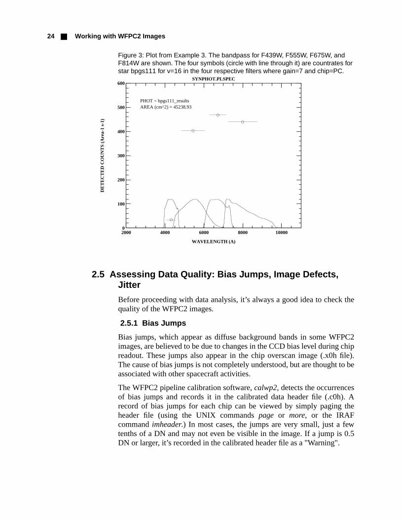
Example 3:

In this example, we plot some results from calcphot. We will determinethe integrated counts in four WFPC2 filters, F439W, F555W, F675W, andF814W in the PC at gain 7, for star #111 in theBruzual-Persson-Gunn-Stryker Atlas (bpgs_111) that’s normalized to aV magnitude of 16.

4000 5000 6000 7000 8000

0

.2

.4

.6

.8

1

WAVELENGTH (A)

PA

SSB

AN

D

SYNPHOT.PLBAND

OBSMODE = wfpc2,f555wOBSMODE = v

WFPC2 Tutorial 23

First, retrieve the table containing the spectra of star bpgs111.

Then, type

calcphot @modes.lis "rn(bpgs_111.fits,band(v),16.0,vegamag)" \

counts out=bpgs111_results

where modes.list is a file containing a list of WFPC2 modes

wfpc2,1,f439w,a2d7

wfpc2,1,f555w,a2d7

wfpc2,1,f675w,a2d7

wfpc2,1,f814w,a2d7

Mode = band(wfpc2,1,f439w,a2d7) Pivot Equiv Gaussian Wavelength FWHM 4312.094 476.4165 band(wfpc2,1,f439w,a2d7)Spectrum: rn(bpgs_111.fits,band(v),16.0,vegamag) VZERO (COUNTS s^-1 hstarea^-1) 0. 34.04943




To plot the results

plspec "" "" counts pfile=bpgs111_results left=2000 right=11000 \

bottom=0 top=600


Figure 3: Plot from Example 3. The bandpass for F439W, F555W, F675W, andF814W are shown. The four symbols (circle with line through it) are countrates forstar bpgs111 for v=16 in the four respective filters where gain=7 and chip=PC.

2.5 Assessing Data Quality: Bias Jumps, Image Defects,Jitter

Before proceeding with data analysis, it’s always a good idea to check thequality of the WFPC2 images.

2.5.1 Bias Jumps

Bias jumps, which appear as diffuse background bands in some WFPC2images, are believed to be due to changes in the CCD bias level during chipreadout. These jumps also appear in the chip overscan image (.x0h file).The cause of bias jumps is not completely understood, but are thought to beassociated with other spacecraft activities.

The WFPC2 pipeline calibration software, calwp2, detects the occurrencesof bias jumps and records it in the calibrated data header file (.c0h). Arecord of bias jumps for each chip can be viewed by simply paging theheader file (using the UNIX commands page or more, or the IRAFcommand imheader.) In most cases, the jumps are very small, just a fewtenths of a DN and may not even be visible in the image. If a jump is 0.5DN or larger, it’s recorded in the calibrated header file as a "Warning".

2000 4000 6000 8000 100000

100

200

300

400

500

600

WAVELENGTH (A)

DE

TE

CT

ED

CO

UN

TS

(Are

a-1

s-1)

SYNPHOT.PLSPEC

PHOT = bpgs111_resultsAREA (cm^2) = 45238.93

WFPC2 Tutorial 25

Depending on your science goals, it may or may not be necessary to correcta bias jump. The following steps outline a procedure for correcting animage affected by a bias jump in one chip. In this example, we use animage (u3b10602t) with a bias jump of 0.589 DN in the WF2. One of thefiles required for the correction is the images’s flat field reference file, andfor this image, it is f4i1559cu.r4h. Also, if the exposure time is less than 10seconds, the shutter shading reference file is needed.

Figure 4: A mosaic of image u3b10602t.c0h (Jupiter taken with filter F160BN15). The left image showsthe bias jump in WF2. On the right, the image has been corrected.

1. From the image display, determine the approximate position of the biasjump in WF2. The bias jump band is seen from y=1 to y=112 in chip2’s coordinate system.

2. Run imstat on the x0h file to get the precise location of the jump. Checkonly columns 5:14 (this is the "good" region in the overscan area that isused for the determining bias level). The following imstat commandswere run in the region where the bias jump was seen to occur. Theresults will help us fine-tune the location where the jump occurs. Createa file named list containing the following image section names

u3b10602t.x0h[2][5:14,110]

u3b10602t.x0h[2][5:14,111]

u3b10602t.x0h[2][5:14,112]

u3b10602t.x0h[2][5:14,113]

u3b10602t.x0h[2][5:14,114]

Bias Jump


Run imstat on the images listed in the file list

imstat @list

The statistics above indicate that the bias jump occurred at y=113.

3. For areas above and below the jump, get the mean value of the pixels.

imstat u3b10602t.x0h[2][5:14,1:112]

imstat u3b10602t.x0h[2][5:14,113:800]

Also get the mean value of all pixels in the overscan areau3b10602t.x0h[2][5:14,1:800].

imstat u3b10602t.x0h[2][5:14,1:800]

In the area before the jump, mean bias value = 352.7 DN

In the area after the jump, mean bias value = 353.3 DN

The mean bias value = 353.2 DN

The difference in bias for the two regions affected by the jump in the imageu3b10602t.c0h[2]:

Line 1 to 112: 352.7 - 353.2 = -0.5 DN

Line 112 to 800: 353.3 - 353.2 = 0.1 DN

IMAGE NPIX MEAN STDDEV MIN MAX

u3b10602t.x0h[2][5:14,110] 10 352.7 0.6749 352. 354.

u3b10602t.x0h[2][5:14,111] 10 352.2 0.6325 351. 353.

u3b10602t.x0h[2][5:14,112] 10 352.8 0.7888 352. 354.

u3b10602t.x0h[2][5:14,113] 10 353.4 0.6992 352. 354.

u3b10602t.x0h[2][5:14,114] 10 353.6 0.6992 353. 355.

# IMAGE NPIX MEAN STDDEV MIN MAX MIDPT

u3b10602t.x0h[2][5:14,1:112] 1120 352.7 0.7028 351. 355. 353.


u3b10602t.x0h[2][5:14,113:800] 6880 353.3 0.7302 351. 356. 353.


u3b10602t.x0h[2][5:14,1:800] 8000 353.2 0.7523 351. 356. 353.

WFPC2 Tutorial 27

4. Create a one-group correction image that will be applied to the WF2image affected by the jump:

• Create a bias "difference" image

imcalc u3b10602t.c0h[2] correct1.hhh "if y .lt. 113 then (0.5) else (-0.1)"

• Apply this correction to the image’s flat field reference file,f4i1559cu.r4h. This is done because the flat-field file, which is nor-malized to 1, is multiplied with the image during the calibrationprocess. Therefore, the same adjustment needs to be made to thebias level corrections that will be applied as well.

imcalc "correct1.hhh,f4i1559cu.r4h[2]" correct2 "im1 * im2"

• If the exposure time is less than 10s, a correction needs to be madeusing the shutter shading reference file. Since the exposure time forthis image was 500 seconds, this correction is unnecessary. But forthe sake of illustrating how the correction is done, assume that theexposure time for this image is 6 seconds. Its shutter shading refer-ence file is e371355eu.r5h. The correction would look like this:

imcalc "correct2,e371355eu.r5h[2]" correct3.hhh "im1 * (1 + im2/6)"

• Create the corrected image

imcopy u3b10602t.c0h[1] corrected_img.hhh[1/4]

imcalc "u3b10602t.c0h[2],correct2" corrected_img.hhh[2] "im1+im2"

imcopy u3b10602t.c0h[3] corrected_img.hhh[3]

imcopy u3b10602t.c0h[4] corrected_img.hhh[4]

(Note: if the exposure time was less than 10 seconds, multiply theWF2 image by the modified shutter shading reference file(correct3.hhh).

2.5.2 Data Quality Files

• For each observation, a set of ascii data quality files are created, withthe extensions .pdq and .trl. The .trl file, generated during pipeline cali-bration, contains a log of calibration steps. The .pdq file contains infor-mation about the actual and predicted observational parameters, andany obvious features that may have been noted by the post-observationprocessing staff. You should page through these files to look for any-thing that would indicate a problem with the data.

• The calibrated science image (extensions .c0h and .c0d) has an associ-ated data quality file (.c1h and .c1d) that provides information about thequality of each pixel in a science image. Bad pixels in the scienceimage are flagged in the data quality image; these flagged pixels aredesignated non-zero positive values indicating the nature of the pixelproblem (listed below). The values in the pixels are additive; a value of3 would indicate a combination of 1 and 2.


How do I determine if any bad pixels fall on critical parts of my scienceimage? Blink the science and data quality images. First, display thescience image, then display the data quality file, and “blink” them.

Hint: When displaying the data quality image (.c1h, .c1d), first runwstatistics on the file to determine the minimum and maximum values. Setthe lower and upper display ranges (z1 and z2 parameters) to match thoseminimum/maximum values (and be sure to set zrange and zscale to “no”).This will produce an image display of the data quality file clearly showingthe bad pixels. A bad pixel’s value can then be determined by placing theimage display cursor on it. Remember that these displayed values are notexact, but are close enough for you to determine what the pixel valueshould be. (For an exact value of a particular pixel, use the task listpix.)

2.5.3 Using Jitter Files to Evaluate Pointing.

The jitter files (also known as Observation Log files) contain informationabout telescope pointing during an observation, as well as relatedengineering data. You might be interested in checking these files if you areconcerned about the quality of the point spread feature in your stellarimage (the FWHM for stars can be measured using imexam.) More detailsabout these files can be found in the HST Data Handbook Appendix(http://www.stsci.edu/hst/HST_overview/documents/datahandbook/) andthe STScI Observatory Support observation log documentation pageat http://www.stsci.edu/instruments/observatory/obslog/OL_1.html

Due to improvements to the jitter files over the history of the telescope,there are different types of file formats available, depending on when theobservations were taken. In this document, we only deal with FITS jitter

Value Description

0 Good pixels.

1 Reed-Solomon decoding error. Pixels in a data packet that were corruptedduring data transmission.

2 Defect in one of the calibration reference files used in calibration or recali-bration. Includes charge transfer traps.

8 A-to-D converter saturation. Signal that is greater than or equal to the maxi-mum A-to-D value (4096).

16 Pixel value was lost during readout or data transmission.

256 Pixels lying above a charge transfer trap that may be affected by the trap.

512 Unrepairable hot pixel.

1024 Repairable hot pixel.


http://www.stsci.edu/instruments/observatory/obslog/OL_1.html

WFPC2 Tutorial 29

files that were generated after 1997. Information about pre-1997 jitter filescan be obtained from the above-mentioned documentation.

Jitter files have the same rootname as the images they are associated with,except that the rootname ends with a j. The information in these files spansnot only the exposure time, but also the pre- and post-observationoverheads starting from the time guide stars were acquired. (Note: the jitterfiles used in this example are in the extension FITS format, and cannot beconverted to GEIS files.)

There are two types of jitter files, ".jif" and ".jit".

1. Jitter files with the". jif" extension contains general pointing informa-tion for the observation.

• The header component of this FITS file contains keywords forguide stars used, pointing and spacecraft jitter, as well as pointinganomalies, if any. Also included is general information about otherobserving parameters such as modelled background light andorbital geometry.

Some useful keywords to check in the .jif file

GUIDECMD Commanded Guiding ModeTNLOSSES Number of loss of lock eventsTLOCKLOS Total loss of lock timeTNRECENT Number of recentering eventsTRECENTR Total recentering timeTV2_RMS RMS jitter along V2 axisTV3_RMS RMS jitter along V3 axisT_ACQ2FL Target acquisition failuresT_GSFAIL Guide star acquisition failuresT_SGSTAR Failure of single star fine lockT_TAPDRP Possible loss of science data

Some keywords will only show up if there’s a problem with theobservation. They include:

GSFAIL The telescope failed to acquire the guide stars.TAPEDROP Potential loss of science dataTLM_PROB A problem with the engineering telemetrySLEWING Slewing occurred during the observationTAKEDATA Take Data Flag NOT on throughout observationSI_PROBnn (where n=1-99) Miscellaneous instrument problems.

A more complete description of these header keywords can befound at http://www.stsci.edu/instruments/observatory/obslog/OL_8.html





Check the guiding mode, number of loss of lock events, and RMSjitter in milliarcseconds along the V2 and V3 axis for all jitter filesin the directory.

hsel *jif.fits[0] $I,GUIDECMD,TNLOSSES,TV2_RMS,TV3_RMS yes

u5ay0701j_jif.fits[0] "FINE LOCK" 0 2.6 3.9u5ay0702j_jif.fits[0] "FINE LOCK" 0 2.6 4.2u5ay0703j_jif.fits[0] "FINE LOCK" 0 3.0 3.7u5ay0704j_jif.fits[0] "FINE LOCK" 0 2.7 4.1u5ay0705j_jif.fits[0] "FINE LOCK" 0 2.6 4.2u5ay0706j_jif.fits[0] "FINE LOCK" 0 2.8 4.3u5ay0707j_jif.fits[0] "FINE LOCK" 0 2.8 4.3u5ay0708j_jif.fits[0] "FINE LOCK" 0 2.7 4.2u5ay0709j_jif.fits[0] "FINE LOCK" 0 2.6 4.1u5ay070aj_jif.fits[0] "FINE LOCK" 0 2.6 4.2

The image portion of the jif file, seen here in Figure 5, shows a64x64 pixel image of the pointing excursion from the center,where the pixel scale is 2 milliarseconds. This 2-dimensionalhistogram indicates that there is slightly more jitter along one axisthan the other (which is normal for most observations).

Figure 5: The image portion of the *jif.fits file showingan image of the pointing excursion from the center.

2. The other kind of jitter file has the extension ".jit". It’s a table contain-ing various values including jitter along V2 and V3, where each jittervalue is an average over a 3 second interval. To get a sense of the jitterduring the observing window, the 3-second-averaged jitter in either theV2 axis or V3 axis can be plotted:

sgraph "u5ay0701j_jit.fits seconds si_v2_avg" # See Figure 6

To look at pointing stability during the observing window, plot the jitterin V2 versus jitter in V3.

sgraph "u5ay0701j_jit.fits si_v2_avg si_v3_avg" # See Figure 7

WFPC2 Tutorial 31

Figure 6: Plot of 3-second-averaged jitter in the V2 axis versus timethat the telescope was pointing at the target for a particular obser-vation (time axis includes pre- and post-observation setup times)

Figure 7: Plot of jitter in V2 vs. jitter in V3, showing the pointing sta-bility during the observing window.

0 100 200 300

-.003

-.002

-1.00E-3

0

seconds [seconds]

si_v

2_av

g [a

rcse

c]

NOAO/IRAF V2.11.3EXPORT [email protected] Tue 14:20:42 05-Feb-2002whimbrel.stsci.e!/data/whimbrel6/tutorial/jitter/u5ay0701j_jit.fits

-.003 -.002 -1.00E-3 0

-.002

0

.002

.004

si_v2_avg [arcsec]

si_v

3_av

g [a

rcse

c]

NOAO/IRAF V2.11.3EXPORT [email protected] Tue 14:30:59 05-Feb-2002whimbrel.stsci.e!/data/whimbrel6/tutorial/jitter/u5ay0701j_jit.fits

32 Calibration and Recalibration

Evaluating pointing accuracy for your observations

There are three different types of guiding scenarios:

1. Two FGS Fine Lock Guiding. This mode uses two guide stars, one ineach of two Fine Guidance Sensors, to lock on a target. Of the threeguiding modes, this produces the most accurate pointing. During anobservation, the pointing can vary by about 1 to 50 milliarcseconds,depending on various spacecraft and observing parameters.

2. Gyro Control. The Rate Gyro Assembly controls pitch, yaw and roll ofthe telescope. Of the three guiding modes, this has the least accuratepointing, producing drifts on the order of 1 to 5 milliarcseconds persecond.

3. Single FGS plus gyro: one guide star is used but the telescope roll iscontrolled by gyros. Errors are about 1 to 5 milliarcseconds per secondof roll about the dominant guide star.

For more information about pointing accuracy and jitter files, please go to

http://www.stsci.edu/instruments/observatory/obslog/OL_7.html#HEADING55

3. Calibration and Recalibration

Data arrives at STScI in the form of original telemetry files (known as"POD" files). Each POD file is partitioned into science and engineeringfiles. It then undergoes various processing steps such as data editing andgeneric conversion, resulting in raw data files (.d0h/.d0d, .q0h/.q0d, etc.).Raw image data is then calibrated with the WFPC2 calibration pipelinesoftware, calwp2, using the best-available calibration reference files.However, these raw and calibrated data files are no longer archived. Aftercertain keyword values and image information are collected for storage in adatabase, the raw and calibrated files are deleted. Later, when a userrequests a particular dataset, the On-the-fly Reprocessing system (OTFR)grabs the dataset’s POD file from the archive, processes it to create rawdata which are calibrated with the best-available reference files usingcalwp2. The raw and calibrated data are then sent to the user.

This section presents an overview of calibration steps for WFPC2 data.Thanks to the OTFR system, all data requested by users are processed withthe latest software, and the best-available calibration reference files, at thetime of the request. Therefore, there’s little reason for users to manuallyrecalibrate their data unless they need to use non-default calibrationreference files.

http://www.stsci.edu/instruments/observatory/obslog/OL_7.html#HEADING55

WFPC2 Tutorial 33

Calibrated data retrieved from the archive within about 2 weeks of anobservation will probably use older dark calibration files. That’s becausedark calibration files for the time of the observations have not yet beencreated -- they are typically available about 2 weeks after the date of theobservation. If you wish to use the best possible dark reference files, youshould check StarView to see if the appropriate dark calibration files foryour observations are ready, and when it is, re-request the data again so thatit can be calibrated with the best dark calibration files.

3.1 Input and Output Files in the Calibration Process

(The file extensions are noted in parenthesis.)

The input data files are:

• Raw data (.d0h, .d0d).

• Data quality files for raw science data (.q0h, .q0d).

• Standard header packet containing observation parameters (.shh, .shd)[Although a part of the raw data set, it is not used by calwp2].

Note: The extracted engineering files (.x0h, .x0d), and its associated dataquality files (.q1h, .q1d) are part of the raw dataset. But they are usedduring calibration and are therefore listed in the next category.

The input calibration reference files are:

• Static mask file (.r0h, .r0d).

• A-to-D (analog-to-digital converter) correction file (.r1h, .r1d).

• Extracted engineering data (.x0h, .x0d), and its data quality file (.q1h,.q1d). [This is the chip overscan area. It’s a component of the rawdataset retrieved from the archive.]

• Bias image reference file (.r2h, .r2d), and its data quality file (.b2h,.b2d).

• Dark image reference file (.r3h, .r3d), and its data quality file (.b3h,.b3d). [Only used for exposures over 10s.]

• Flat field file (.r4h, .r4d), and its data quality file (.b4h, .b4d).

• Shutter shading correction (.r5h, .r5d). [Only used for exposures under10s.]

• HST Graphs Table (.tmg) and Components Table (.tmc), throughputtables used to determine photometric information for a dataset.


After running calwp2, output files are:

• Calibrated science data (.c0h, .c0d).

• Data quality files for calibrated science data (.c1h, .c1d).

• Histogram of good science data pixel values (.c2h, .c2d) [optional].

• Photometric throughput table for the dataset (.c3t).

• ASCII file containing group parameters and their values (.cgr).

Data obtained from the archive also include:

• File containing group parameters in ASCII format. It’s only used in thepipeline and is not needed if you recalibrate your data. (.dgr)

• The Standard Header Packet, not used by calwp2 but it’s part of thestandard WFPC2 dataset. (.shh, .shd)

3.2 The Calibration Steps

Each individual calibration step can be executed by setting a “switch” inthe raw data header file. This way, if a particular calibration step isunnecessary, it does not have to be performed when you recalibrate the datausing calwp2.

What are the calibration steps?

Each calibration step is listed below in the order it is done:

1. The static mask reference file (.r0h, .r0d) identifies charge transfertraps and other pixels affected by the traps. This information is enteredin the calibrated image data quality file (.c1h, .c1d). The image data(.c0h, .c0d) itself is not changed.

The header keyword switch is MASKCORR.The header keyword indicating the calibration filename is MASKFILE.

2. The A-to-D reference file (.r1h, .r1d) corrects each pixel value of thescience data for analog-to-digital conversion errors.

The header keyword switch is ATODCORR.The header keyword indicating the calibration filename is ATODFILE.

3. A mean bias level is subtracted from each pixel in the science image.This value, one for each chip, is derived from a subset of the overscanregion for that chip. The overscan regions are stored in the extractedengineering file (.x0h, .x0d). (Its data quality file (.q1h, .q1d) con-tains bad pixel information that is also flagged in the calibrated sciencedata quality file (.c1h, .c1d).)

The header keyword switch is BLEVCORR.

WFPC2 Tutorial 35

The header keyword indicating the calibration filename is BLEVFILE.The header keyword indicating the calibration data quality filename isBLEVDFIL.

4. Position-dependent bias patterns are subtracted from the science datausing the bias pattern reference file, also referred to as the superbiasfile (.r2h, .r2d). Bad pixels in the bias pattern reference file arerecorded in its data quality file (.b2h, .b2d), and are also flagged in thescience data quality file (.c1h, .c1d) during calibration.

The header keyword switch is BIASCORR.The header keyword indicating the calibration filename is BIASFILE.The header keyword indicating the calibration data quality filename isBIASDFIL.

5. The dark reference file (.r3h, .r3d), and its data quality file (.b3h,.b3d), are generated about every week. Dark reference files are onlyneeded for observations where the header keyword DARKTIME isgreater than 10s.

The header keyword switch is DARKCORR.The header keyword indicating the calibration filename is DARKFILE.The header keyword indicating the calibration data quality filename isDARKDFIL.

6. The science image is multiplied with a flat field reference image (.r4h,.r4d). Information about bad pixels in the flat field reference image isfound in its data quality file (.b4h, .b4d), and flagged in the scienceimage data quality file (.c1h, .c1d) during calibration.

The header keyword switch is FLATCORR.The header keyword indicating the calibration filename is FLATFILE.The header keyword indicating the calibration data quality filename isFLATDFIL.

7. For exposures less than 10 seconds, a shutter shading correction file(.r5h, .r5d) must be applied to the science data. This is necessarybecause the finite shutter velocity creates a “shading” effect in theimage. This shading effect also depends on which of the two shutters isused (either shutter A or B).

The header keyword switch is SHADCORR.The header keyword indicating the calibration filename is SHADFILE.

8. In order to populate photometry-related keywords in the calibrated sci-ence header files, set the keyword switch DOPHOTOM in the “.d0h”file to PERFORM. During calibration, values for the following key-words will be calculated using Synphot:


PHOTMODEPHOTFLAMPHOTPLAMPHOTBWPHOTZPT

This step uses two tables, a graph table (.tmg) and a component table(.tmc) containing telescope and instrument throughput information.These tables are often updated for all on-board HST instruments as newresults from ongoing calibration activities become available. To findout the names of the latest WFPC2 throughput tables, see the WFPC2Synphot memo at

http://www.stsci.edu/ftp/instrument_news/WFPC2/Wfpc2_phot/wfpc2_synphot.html#summary

For example, as of February 6, 2002, the latest WFPC2 throughputtables were

m1p1255om_tmg.fitsm1s1421hm_tmc.fits

This calibration step will not change the pixel data values, it will onlypopulate the header photometry keywords. This is useful for peoplewho plan to use a flux-based photometric system such as the AB orSTMAG system. More information about different photometricsystems can be found in section 4 and the WFPC2 Data Handbook.

In addition, a throughput table (.c3t) will be created by calwp2 usingthe synphot program.

The header keyword switch is DOPHOTOM.The header keywords indicating the calibration tables are GRAPHTABfor the graph table (.tmg), and COMPTAB for the components table(.tmc).

9. An optional calibration step is to generate a file containing histogramsof raw data, A-to-D corrected data, and the final calibrated output datafor each group. This file (.c2h, .c2d) will contain histograms of rawdata in row 1, A-to-D corrected data in row 2, and the final calibrateddata in row 3.

The header keyword switch is DOHISTOS.

10. The image datatype is specified in the input image header file.

The header keyword is OUTDTYPE, and can be set to either REAL,LONG or SHORT.

Note: During the calibration process, calwp2 detects saturated pixels in theraw image file (.d0h, .d0d), and flags them in the calibrated data quality file

http://www.stsci.edu/ftp/instrument_news/WFPC2/Wfpc2_phot/wfpc2_synphot.html#summary

WFPC2 Tutorial 37

(.c1h, .c1d). Therefore, the keyword switch DOSATMAP, which creates animage map of saturated pixels is unnecessary, and may be set to OMIT.

More information on the calibration steps can be obtained from theWFPC2 section in the HST Data Handbook for WFPC2, version 4.0,located at http://www.stsci.edu/instruments/wfpc2/Wfpc2_dhb/WFPC2_longdhbcover.html

3.3 The Calibration ProcedureRecalibrating the dataset u5ay0701r

StarView, can be used to determine which reference files should be used forrecalibration; at the Searches menu item go to STScI --> Instruments -->WFPC2 --> WFPC2 Reference Files. Enter the dataset in the table-likesection at the top of the search window. Or you can search for the referencefile you want to use at Searches --> STScI --> Instruments --> WFPC2 -->WFPC2 Calibration Data.

Example: Calibration reference files needed for u5ay0701r:

Each calibration step will be executed in calwp2 if the input image headerkeyword “switch” is set to PERFORM. The step will not be executed if the“switch” is set to OMIT. The next listing shows an excerpt of a raw dataheader file (.d0h) with the calibration keyword switches.

Type of Calibration Calibration Header Filename Switch (recommended)

A-to-D Correction: DBU1405IU.R1H perform

Bias Correction: KCD1557LU.R2H perform

Dark Current Correction: JAE1431QU.R3H perform

Flat Field Correction: G640925NU.R4H perform

Static Pixel Mask: F8213081U.R0H perform

Shutter Shading File: E371355IU.R5H omit

Engineering File: U5AY0701R.X0H perform

Photometric Calibration Table: U5AY0701R.C3T perform

Graph Table: M1P1255OM_TMG.FITS

Components Table: M1S1421HM_TMC.FITS

http://www.stsci.edu/instruments/wfpc2/Wfpc2_dhb/WFPC2_longdhbcover.html



The following is an excerpt from the raw data header file, u5ay0701r.d0h,listing the calibration reference files (uref, ucal, and mtab are IRAFpointers to files -- more on this later):

How do I set the new reference files and switches for recalibration?

Before running calwp2, the appropriate calibration files and calibration“switches” have to be set in the raw image header file (.d0h,). One way todo this is using the task chcalpar (found in the packagestsdas.hst_calib.ctools).

chcalpar (CHange CALibration PARameters) is an easy way to edit GEISheader files. It is actually a task that calls other related tasks called “psets”.When chcalpar is executed, it looks at the data to determine whichinstrument was used. Since our datasets are WFPC2 images, chcalpar willcall the pset ckwwfp2 to edit the raw image header file.

/ RSDP CONTROL KEYWORDSMASKCORR= ’PERFORM ’ / Do mask correction: PERFORM, OMIT, COMPLETEATODCORR= ’PERFORM ’ / Do A-to-D correction: PERFORM, OMIT, COMPLETEBLEVCORR= ’PERFORM ’ / Do bias level correctionBIASCORR= ’PERFORM ’ / Do bias correction: PERFORM, OMIT, COMPLETEDARKCORR= ’PERFORM ’ / Do dark correction: PERFORM, OMIT, COMPLETEFLATCORR= ’PERFORM ’ / Do flat field correctionSHADCORR= ’OMIT ’ / Do shaded shutter correctionDOSATMAP= ’OMIT ’ / Output saturated pixel mapDOPHOTOM= ’PERFORM ’ / Fill photometry keywordsDOHISTOS= ’OMIT ’ / Make histograms: PERFORM, OMIT, COMPLETEOUTDTYPE= ’REAL ’ / Output image datatype: REAL, LONG, SHORT

/CALIBRATIONREFERENCEFILESMASKFILE= ’uref$f8213081u.r0h ’ / name of the input DQF of known bad pixelsATODFILE= ’uref$dbu1405iu.r1h ’ / name of the A-to-D conversion fileBLEVFILE= ’ucal$u5ay0701r.x0h ’ / Engineering file with extended register daBLEVDFIL= ’ucal$u5ay0701r.q1h ’ / Engineering file DQFBIASFILE= ’uref$kcd1557lu.r2h ’ / name of the bias frame reference fileBIASDFIL= ’uref$kcd1557lu.b2h ’ / name of the bias frame reference DQFDARKFILE= ’uref$jae1431qu.r3h ’ / name of the dark reference fileDARKDFIL= ’uref$jae1431qu.b3h ’ / name of the dark reference DQFFLATFILE= ’uref$g640925nu.r4h ’ / name of the flat field reference fileFLATDFIL= ’uref$g640925nu.b4h ’ / name of the flat field reference DQFSHADFILE= ’uref$e371355iu.r5h ’ / name of the reference file for shutter shaPHOTTAB = ’ ’ / name of the photometry calibration tableGRAPHTAB= ’mtab$k4j0855mm_tmg.fits’ / the HST graph tableCOMPTAB = ’mtab$m1a15296m_tmc.fits’ / the HST components table

WFPC2 Tutorial 39

Example

chcalpar u5ay0701r.d0h

This command will call the WFPC2 pset ckwwfp2 which will list all thedefault header keyword switches and reference files for u5ay0701r.d0h:

• Edit the parameters to enter new reference filenames and switch set-tings, based on recommendations from StarView, or from the WFPC2reference file memo located at

http://www.stsci.edu/ftp/instrument_news/WFPC2/Wfpc2_memos/wfpc2_reffiles.html

When completed, type :q

• The screen will reappear, but this time, the fields will be blank exceptfor the new entries. Verify that the changes are correct and enter addi-tional changes if necessary. When completed, type :q

PACKAGE = ctools TASK = ckwwfp2(maskcor= perform) >do mask correction?(atodcor= perform) >Do A-to-D correction?(blevcor= perform) >do bias level correction?(biascor= perform) >do bias correction?(darkcor= perform) >do dark correction?(flatcor= perform) >do flat field correction?(shadcor= omit) >Do shaded shutter correction?(dophoto= perform) >fill photometry keywords?(dohisto= omit) >Make histograms?(outdtyp= real) >output image data type?(maskfil= uref$f8213081u.r0h) >name of the input DQF of known bad pixels(atodfil= uref$dbu1405iu.r1h) >name of the A-to-D conversion(blevfil= ucal$u5ay0701r.x0h) >engineering file with extended register data(blevdfi= ucal$u5ay0701r.q1h) >engineering file DQF(biasfil= uref$kcd1557lu.r2h) >name of the bias frame reference file(biasdfi= uref$kcd1557lu.b2h) >name of the bias frame reference DQF(darkfil= uref$jae1431qu.r3h) >name of the dark reference file(darkdfi= uref$jae1431qu.b3h) >name of the dark reference DQF(flatfil= uref$g640925nu.r4h) >name of the flat field reference file(flatdfi= uref$g640925nu.b4h) >name of the flat field reference DQF(shadfil= uref$e371355iu.r5h) >name of the reference file for shaded shutter c(phottab= ) >name of the photometry calibration table(graphta= mtab$k4j0855mm_tmg.fits)>the HST graph table(comptab= mtab$m1a15296m_tmc.fits)>the HST components table(instrum= wfpc2) Instrument represented by this pset(Version= 14Feb94) Date of Installation(mode = a)

http://www.stsci.edu/ftp/instrument_news/WFPC2/Wfpc2_memos/wfpc2_reffiles.html


• A prompt will appear asking “accept current parameters?” with theoptions no, yes, and abort. If you wish to proceed in entering the newreference filenames and switches in the raw image header file (.d0h),type yes

Please refer to the STSDAS on-line help files calwp2, ckwwfp2, andchcalpar for more details.

How do I run calwp2?

• Before running calwp2, be sure that pointers to the location of refer-ence files are set up properly. uref$, ucal$, and mtab$ are pointers todirectories where reference files are stored. They are prefixes to the cal-ibration filenames specified in the image header. These pointers mustbe set before running calwp2.

As an example, assume the raw data are located at/data/whimbrel1/science/, and calwp2 will be run in that directory. Andassume all reference files are located at /data/whimbrel1/ref/. In IRAF,set the pointers by typing

set uref = /data/whimbrel1/ref/

set ucal = /data/whimbrel1/science/

set mtab = /data/whimbrel1/ref/

(Note: that final "/" is important! Don’t forget it.)

You can verify that the pointers were set correctly by using the IRAFshow command,

show uref

gives

/data/whimbrel1/ref/

After doing this, running calwp2 is easy. At the IRAF prompt, type

calwp2 u2g40o05t ""

In this example, the calibrated science data will have the samerootname as the raw science data, with the c0h/.c0d extension.

3.4 A Closer Look at the Calibration Process

What happens to the pixels at each stage of the calibration process?

The best way to understand the calibration process is to manually performeach step in the calibration pipeline, tracing a couple of pixels from thebeginning to the end of the process. To do this, pick two unsaturated pixelsin your raw science image, (x1,y1) and (x2,y2), and make a note of theirraw data values, and location in their chip.

WFPC2 Tutorial 41

1. Perform the mask correction

What are the new science data pixel values?Background: The static pixel mask reference file contains a map of per-manently bad pixels. Currently, only two types of bad pixels areflagged: charge transfer traps (assigned the value 2) and pixels abovecharge transfer traps that are affected by the traps (assigned the value256). This mask file is copied to the calibrated data quality file (.c1h,.c1d).Hint: The mask correction only updates the data quality file (.c1h, .c1d)with information about bad pixels. The science data is not changed. Butbe sure to check (x1,y1) and (x2,y2) to make sure they are not affectedby the traps.

2. Perform the A-to-D correction

What are the new science data pixel values?Background: Each CCD pixel absorbs energy from photons of light thatimpinge upon it, releasing electrons within the semiconductor. Theaccumulated electrons from a particular pixel are trapped in a specificlocation corresponding to that pixel. The analog-to-digital converter(ADC) is a device that converts the CCD pixel voltage signal (fromtrapped electrons) to Data Numbers (DNs) that can be stored in com-puter memory. For the WFPC2, the ADC has a range of 12 bits -- 4096possible values ranging from 0 to 4095. In order to effectively “scale”the accumulated signal for storage, users can specify a gain of 7 elec-trons/DN or 14 electrons/DN. The choice of gain setting depends on thescientific objectives of the observations. (For more information, see theWFPC-2 Instrument Handbook (version 6.1), page 79-81, and for ageneral overview of CCDs, please refer to Electronic and Com-puter-aided Astronomy: From Eyes to Electronic Sensors, by IanMcLean.)The A-to-D converter has a known problem; certain DN values arereported more (or less) frequently than a perfect device. The A-to-Dconverter therefore produces small errors when converting from elec-trons to DN values. Although the “true” DN values can never be recov-ered, the errors are systematic and a statistical correction can beapplied. (The largest correction for WFPC2 is 0.1%.)In theory, the A-to-D correction is a function of temperature. TheA-to-D conversion reference file is a matrix of values for each chip; thefirst row contains possible temperature values for Bay 3. The secondand subsequent rows, with each row corresponding to a particular tem-perature, contain A-to-D conversion corrections for each DN valuebetween 0 to 4095.The example below illustrates the structure of an A-to-D converter cor-rection file with conversion values for five different temperatures. The


first row has 5 temperature values, t1 to t5. The second row has the DNcorrections corresponding to temperature t1 -- there are 4096 columns,with the first column containing the correction value for a raw DNvalue of 0, and 4096th column containing the correction for the rawDN value of 4095. The third row has the corrections for temperature t2,the 4th row for temperature t3, etc.

(col 1) (col 2) (col 3) (col 4) (col 5) . . . . . . . . (col 4096)(row 1) ---- t1 t2 t3 t4 t5(row 2) 0_t1 1_t1 2_t1 3_t1 4_t1 . . . . . . . . 4095_t1(row 3) 0_t2 1_t2 2_t2 3_t2 4_t2 . . . . . . . . 4095_t2(row 4) 0_t3 1_t3 2_t3 3_t3 4_t3 . . . . . . . . 4095_t3(row 5) 0_t4 1_t4 2_t4 3_t4 4_t4 . . . . . . . . 4095_t4(row 6) 0_t5 1_t5 2_t5 3_t5 4_t5 . . . . . . . . 4095_t5

The A-to-D reference file was created from data taken during WFPC2Thermal Vacumn tests before launch. On-orbit checks have determinedthat the conversion values have remained constant. Therefore, only theconversion values for a single temperature setting is necessary. Currentreference files have the dimension 4096x2. Row 1 has one temperatureentry, at [2,1], and all other values in row 1 are set to -1 (null value).Row two is the lookup table for this temperature, and has 4096columns.

Example:

Determine the A-to-D correction for a DN value of 317 for the WF2chip.

This correction can be found in group 2 of the A-to-D reference file,at location [317+1,2]. The task listpix can be used to obtain thecorrect DN value to be substituted in the calibrated data files (.c0h,.c0d).

listpix dbu1405iu.r1h[2][318,2]

1. 316.9859

During the A-to-D correction step in the calibration, all DN values of317 in group 2 of the raw image data are changed to 316.9859.

3. Perform the bias level correction

What are the global bias values for even (BIASEVEN) and odd(BIASODD) columns?

What are the science data pixel values (x1,y1) and (x2,y2) aftersubtracting its global bias value?

Background: A pedestal of about 300 DN is introduced into the signalchain to prevent the occurrence of negative numbers. A mean value forthis bias level can be obtained in the CCD overscan region stored in theengineering files (.x0d, .x0h) that accompanies each WFPC2 dataset.

WFPC2 Tutorial 43

(The overscan area is obtained as the CCD electronics continues toread-out even though there is no longer any physical correspondence tothe chip.)

The mean bias value is slightly different for even and odd columns.During calibration, mean bias values are determined for the even andodd columns of the science image, derived using a subsection of theoverscan region. These values are stored in the science image headerkeywords BIASEVEN and BIASODD, respectively. The mean biaslevels are then subtracted from the science image; the BIASEVENvalue from even columns of the science image, and the BIASODDvalue from the odd columns of the science image.

The mean bias levels are calculated from a subsection of the overscanimage (.x0h,.x0d) at [9:14,10:790]. Columns 9, 11, and 13 in theoverscan region are used to obtain the BIASEVEN value. Columns 10,12, and 14 are used to derive a value for BIASODD. (Thisnomenclature, where odd columns in the engineering file are used todetermine the mean bias level of even columns in the science image,and vice versa, is due to an offset between the overscan region and theimage.)

Hints:

- Determine if (x1,y1) and (x2,y2) in the science image fall on evenor odd columns.

- Determine the mean bias level for even and odd columns(BIASEVEN and BIASODD) for each chip, using the overscanregion of that chip in the engineering file (.x0d, .x0h). Use a tasklike imstat to get mean values of the appropriate sections in theoverscan image.

- Subtract the bias level (either BIASEVEN or BIASODD) from thevalue of the science data pixel, depending on whether the imagepixel falls in an even or odd column.

4. Perform a bias correction

What are the pixel values in the bias correction file?

What are the new science data pixel values?

Background: After subtracting the global bias values from the image,there still remains small scale bias values that vary from pixel-to-pixel.These are removed by subtracting a bias correction reference image(.r2h, .r2d) from the science image. This bias reference file, or“superbias,” is generated annually using 120 individual bias frames thatwere corrected for A-to-D conversion errors, with global bias levelssubtracted.


Hint: Look up the pixel values in the bias correction file (.r2h, .r2d) atpositions (x1,y1) and (x2,y2). Subtract that bias correction value fromthe science data pixels.

5. Perform a dark correction

What are the pixel values in the dark file?


Background: Thermally-induced dark currents, as well as a faint“glow” caused by cosmic rays striking the corrector plates, make darkcorrections necessary for exposures greater than 10 seconds. Thiscorrection is done by subtracting a dark reference image from thescience image.

The dark reference image has two components: one is a “superdark”generated annually from 120 individual dark images. The second is hotpixel information derived from five darks taken during the week of thescience observations. Therefore, a new dark reference file is generatedevery week using that year’s superdark, but containing weekly-updatedhot pixel information. If the data is retrieved shortly after theobservations were taken, the dark reference file may be out-of-date bya couple of weeks. The user could either recalibrate the data with a newdark reference file when it becomes available, or re-request the datafrom the archive when the correct dark reference file is in the archive(which can be checked using StarView).

Each dark reference image is normalized to a 1 second exposure time.Therefore, when it is applied to the science data, the dark file is firstscaled to the science image by multiplying it with the DARKTIMEkeyword value in the raw science data header file (.d0h). (DARKTIMEis defined as the total time from the start of an exposure to thebeginning of readout. The pipeline approximates this “darktime” bysetting it equal to the exposure time.)

Hint: Look up the pixel values of (x1,y1) and (x2,y2) in the darkreference file. Remember that the dark file has been normalized to 1second. Therefore, to correct for exposure time, look up the keywordDARKTIME in the raw image header file. Multiply the dark file pixelvalue by the DARKTIME value. Then, subtract the correctly-scaleddark value from the science data pixel value.

6. Flat field the image

What are the pixel values in the flat field image?


Background: The photometric response in the science image variesover the field-of-view. There are several reasons for this effect. Each

WFPC2 Tutorial 45

CCD pixel has its own unique quantum efficiency. Each chip has aslightly different electronic gain. Large-scale vignetting of the field iscaused by the telescope and WFPC2 mirrors, their support structures,and WFPC2 filters. Optical distortions are introduced by field flattenersin front of each chip, causing the sky area per pixel at a chip corner tobe about 5% smaller than at the chip center. A manufacturing defectaffecting every 34th row in the CCDs also reduces sky coverage perpixel. Even dust particles on the pyramid, CCD windows, and detectorscause artifacts. Most electronic effects were characterized duringpre-launch thermal vacuum testing, while large-scale optical effectswere determined from on-orbit Earth flats. The flat field file corrects forthese sensitivity variations in the science image.

Hint: Look up the pixel values for (x1,y1) and (x2,y2) in the flat fieldfile. Multiply the science pixel values with their corresponding flat fieldpixel values. (Note: The flat fields have been inverted to be consistentwith other multiplicative reference files used in the pipelinecalibration.)

7. Shutter Shading Correction

Was a shutter shading correction necessary for this dataset?

Background: The WFPC2 has two shutter blades. When an exposurebegins, one shutter blade is moved off the light path. The exposure endswhen the second shutter blade moves to block the light path. Althoughthe blades move rapidly, their finite motion can cause exposure timevariations over the field-of-view for total exposure times of 1 second orless. The calibration software automatically applies a shutter shadingcorrection to images with total exposure times less than 10 seconds.The two shutters have slightly different speeds; therefore, there are twodifferent correction files depending on which blade was moved out ofthe way at the beginning of the exposure.

Hint: Exposure times less than 10 seconds require a shutter shadingcorrection. Below is an example of applying this correction using theIRAF task imcalc:

imcalc sci_image, shutter out_image “im1 * (1 + (im2 / <exposure time>))”

As a final check, compare the (x1,y1) and (x2,y2) values from thestep-by-step calibration with the pixel values in thepreviously-calibrated images. Do they agree to 3 decimal places? If“no”, you may want to check your steps for errors.

46 Photometry: Converting DNs to a Magnitude

4. Photometry: Converting DNs to a Magnitude

4.1 Some General Notes about WFPC2 Photometry

This section illustrates the use of aperture photometry to obtain V and Imagnitudes of stars in the LMC star cluster NGC 2100. Other topics inphotometry, such as PSF-fitting, surface, and narrow-band photometry, arenot covered here. For more details on these topics, please refer to thefollowing sources of information:

PSF-fitting Photometry:

Peter Stetson’s DAOPHOT package can be found at

http://iraf.noao.edu/iraf/web/irafnews/dec94/dec94-S-27.html or

http://hires.gsfc.nasa.gov/~beck/pkgs/daophot2.html

Andrew Dolphin’s HSTPhot, is specifically for WFPC2 data, and usesTinyTim PSFs at different locations on the WFPC2 chips.

http://www.noao.edu/staff/dolphin/hstphot/

DoPHOT, written by Mario Mateo, Abi Saha and Paul Schechter, searchesfor "objects", and produces positions, magnitudes, and crudeclassifications. The paper describing DoPHOT can be found at

http://adsbit.harvard.edu/cgi-bin/nph-iarticle_query?bibcode=1993PASP..105.1342S

The DoPHOT page is at

http://arcturus.mit.edu:80/~schech/dophot.html

Ken Mighell’s MATPHOT does PSF-fitting CCD stellar photometry.

http://www.noao.edu/staff/mighell/matphot/

John Krist’s Tiny Tim Software for creating simulated PSFs.

http://www.stsci.edu/software/tinytim/tinytim.html

Narrow-band Photometry:

FAQ located at

http://www.stsci.edu/instruments/wfpc2/Wfpc2_faq/wfpc2_nrw_phot_faq.html

Surface Photometry:

STSDAS has a software package for surface photometry called isophote(stsdas.analysis.isophote). Please refer to the on-line help files for moreinformation on this method.

http://iraf.noao.edu/iraf/web/irafnews/dec94/dec94-S-27.html�

http://www.noao.edu/staff/dolphin/hstphot/

http://adsbit.harvard.edu/cgi-bin/nph-iarticle_query?bibcode=1993PASP..105.1342S

http://arcturus.mit.edu:80/~schech/dophot.html

http://www.noao.edu/staff/mighell/matphot/

http://www.stsci.edu/software/tinytim/tinytim.html

http://www.stsci.edu/instruments/wfpc2/Wfpc2_faq/wfpc2_nrw_phot_faq.html

http://iraf.noao.edu/iraf/web/irafnews/dec94/dec94-S-27.html�



http://iraf.noao.edu/iraf/web/irafnews/dec94/dec94-S-27.html

WFPC2 Tutorial 47

Useful aperture photometry links:

Photometry with the WFPC2 by Brad Whitmore


WFPC2 Photometry Cookbook by Brad Whitmore


The Photometric Performance and Calibration of WFPC2, by Holtzman, etal., 1995.


WFPC2 ISR 95-04: A Demonstration Analysis Script for PerformingAperture Photometry by Brad Whitmore and Inge Heyer

http://www.stsci.edu/instrument-news/isr/wfpc2/9504/9504_1.html

Ken Mighell’s QDPHOT page.

http://www.noao.edu/noao/staff/mighell/qdphot/

CCDCAP: CCD Circular Aperture Photometry, also by Ken Mighell

http://www.noao.edu/noao/staff/mighell/ccdcap/

4.2 WFPC2 Photometric Systems

The magnitude is defined as

m= -2.5log10(DN/exptime) + zeropoint

where the zeropoint of an instrument, by definition, is the magnitude of anobject that produces one count (or one DN) per second.

The zeropoint can be determined using four ways:

1. From your own ground-based photometry, using standard filters, ofobjects in the field (if available).

2. Using the zeropoints published by Jon Holtzman in The PhotometricPerformance and Calibration of WFPC2, PASP 1995, (a link to thispaper can be found in http://www.stsci.edu/instruments/wfpc2/wfpc2_doc.html#Phot). These zeropoints are known as the WFPC2 Flight Pho-tometric System. It was established to match the standardJohnson-Cousins UBVRI system such that the magnitudes of Vega inthe standard U, B, V, R, and I filters are the same as the magnitudes inthe closest equivalent WFPC2 filters (F336W, F439W, F555W, F675W,and F814W respectively).

Holtzman et al. also provides transformation coefficients to convert theWFPC2 Flight Photometric System to standard UBVRI magnitudes,but warns that the transformations can be highly uncertain. Updated



http://www.noao.edu/noao/staff/mighell/qdphot/



http://www.noao.edu/noao/staff/mighell/ccdcap/




photometric zeropoints have recently been provided by Andrew Dol-phin, and can be found on his website at http://www.noao.edu/staff/dol-phin/wfpc2_calib/. Note: Both Holtzman and Dolphin zeropoints areapplied to magnitudes in an aperture radius of 0.5".

3. Another set of zeropoints was published by Whitmore and Heyer inInstrument Science Report 96-04, and later updated in the HST DataHandbook. (Future zeropoints updates will be announced in theWFPC2 Space Telescope Analysis Newsletter (STAN) and posted onthe WFPC2 website. These zeropoints are defined such that Vega has amagnitude of zero for all WFPC2 filters. Note: these zeropoints areapplied to magnitudes in an "infinite" aperture, which is defined as themagnitude in a 0.5" aperture - 0.1 magnitude.

The magnitude of Vega in the Holtzman system, and in the system orig-inally defined by Whitmore and Heyer, are summarized in the tablebelow:

4. The PHOTFLAM image header keyword value is the flux of a sourcewith constant flux per unit wavelength (in ergs s-1 cm-2 A-1) that pro-duces a count rate of 1 DN per second. This keyword is useful for con-verting the counts directly to a flux density, or to a flux-based systemsuch as the AB system or the STMAG system. Please refer to theWFPC2 HST Data Handbook for more details.

4.3 From DNs to Instrument Magnitudes: A PhotometryDemo

The following sections illustrate one of several different stellar aperturephotometry methods. It is by no means a standard technique, but instead,an introduction that will provide a foundation for exploring different typesof stellar photometry methods.

This example is a step-by-step procedure for measuring the magnitudes ofstars in the NGC 2100 field in the PC, using filters F555W and F814W. Thedatasets used are

F555W: u5ay0701r, u5ay0702rF814W: u5ay0704r, u5ay0705r

WFPC2 Flight Photometric System (Holtzman et al. ’95) Whitmore-Heyer SystemU(Johnson-Cousins)=0.02 F336W(WFPC2 Flight)=0.02 U(Vegamag)=0 F336W(Vegamag)=0B(Johnson-Cousins)=0.02 F439W(WFPC2 Flight)=0.02 B(Vegamag)=0 F439W(Vegamag)=0V(Johnson-Cousins)=0.03 F555W(WFPC2 Flight)=0.03 V(Vegamag)=0 F555W(Vegamag)=0R(Johnson-Cousins)=0.039 F675W(WFPC2 Flight)=0.039 R(Vegamag)=0 F675W(Vegamag)=0I (Johnson-Cousins)=0.035 F814W(WFPC2 Flight)=0.035 I (Vegamag)=0 F814W(Vegamag)=0

http://www.noao.edu/staff/dolphin/wfpc2_calib/



WFPC2 Tutorial 49

Place the images in two separate directories, one for each filter. First of all,get some basic information about these image, such as exposure time,A-to-D gain, and filters used:

hselect "u5ay0701r.c0h, u5ay0702r.c0h" $I,exptime,atodgain,filtnam1,filtnam2 yes

u5ay0701r.c0h 3.500000000000E+02 7.0 F555Wu5ay0702r.c0h 3.500000000000E+02 7.0 F555W

hselect "u5ay0704r.c0h, u5ay0705r.c0h" $I,exptime,atodgain,filtnam1,filtnam2 yes

u5ay0704r.c0h 3.500000000000E+02 7.0 F814Wu5ay0705r.c0h 3.500000000000E+02 7.0 F814W

In this example, the aperture photometry task apphot will be used. Thispackage is available in IRAF. It can be loaded by typing

noao

digiphot

apphot

4.3.1 Combine the Image Pairs

Determine if the image pairs for each filter are registered. This can be doneby blinking the images, or by measuring the position of several stars (usingimexam) in each image to verify that their coordinates are identical. Ingeneral, consecutive observations with the same pointing using the sameguide stars will show no offsets. But if the exposure is long, and one of theFine Guidance Sensors loses track of its guide star, a small drift in thetelescope roll is possible, resulting in a slightly trailed image. Suchproblems are always documented in the data quality reports (.pdq files) thataccompany each dataset, retrievable from the archive.

The images have the same pointing, and we will use the task crrej tocombine the images. (Other available tasks for WFPC2 image combinationare stsdas.hst_calib.wfpc.combine and stsdas.toolbox.imgtools.gcombine.)

First, save a copy of the data quality files (.c1h, .c1d) because crrej willchange some values when it flags cosmic rays (with ID=128). Then,combine the images. Be sure to use the correct setting for the A-to-D gainand readnoise (in DN) parameters. Otherwise, default settings have beenused for other parameters in this example.

In the F555W directory:

!mkdir backup_dq

!cp *.c1h *.c1d backup_dq/

unlearn crrej

crrej "u5ay0701r.c0h,u5ay0702r.c0h" f555w_temp.hhh \

"u5ay0701r.c0h,u5ay0702r.c0h" "8,6,4" atodgain=7 readnoise=0.72 crdqval=128


In the F814W directory:

!mkdir backup_dq

!cp *.c1h *.c1d backup_dq/

unlearn crrej

crrej "u5ay0704r.c0h,u5ay0705r.c0h" f814w_temp.hhh \

"u5ay0704r.c0h,u5ay0705r.c0h" "8,6,4" atodgain=7 readnoise=0.72 crdqval=128

Note: Many WFPC2 images are now dithered to remove hot pixels and toobtain better pixel resolution. For more information on how to reducedithered images, please refer to the Dither Handbook, edited by AntonKoekemoer, located at

http://www.stsci.edu/instruments/wfpc2/Wfpc2_driz/dither_handbook.html.

4.3.2 Correct the Images for Geometric Distortion

The WFPC2 camera optics introduces a geometric distortion to the fieldthat affects astrometry and photometry. The affect on surface photometry isremoved in the pipeline when the images are multiplied by flat fields. Butfor point source photometry, a correction needs to be applied as a functionof the position of the object in the field. (For more information, please referto the paper by Holtzman et al., Performance and Calibration of WFPC2 onthe Hubble Space Telescope, especially Figure 16.) A geometric correctionimage (for all four chips) was generated by the WFPC2 InstrumentDevelopment Team, called f1k155bu.r9h, that can be retrieved from thephotometry section of the WFPC2 home page at

http://www.stsci.edu/instruments/wfpc2/Wfpc2_memos/wfpc2_reffiles.html#Pixel

Note: There is a wavelength dependence in the distortion in the UV. Detailsregarding corrections for other filters can be found in the paper “Geometryof the WFPC2 Focal Plane” by Trauger et al. in Calibrating Hubble SpaceTelescope: Post Servicing Mission, a Workshop held on May 15 - 17, 1995(contact [email protected] to request a paper copy). A new geometricdistortion solution for F555W is also available: please see ISR 2001-10: AnImproved Geometric Solution for WFPC2 by Casertano and Wiggs.

The simplest way to apply this correction is to multiply your image byf1k155bu.r9h. In the F555W directory,

imcalc "f555w_temp.hhh,f1k1552bu.r9h" f555w.hhh "im1*im2"

In the F814W directory,

imcalc "f814w_temp.hhh,f1k1552bu.r9h" f814w.hhh "im1*im2"

4.3.3 Create a Coordinate List for the Stars

Since the F555W and F814W images were obtained at the same pointing,one coordinate list will be used. This coordinate list will be generated usingthe task daofind, which is part of the apphot aperture photometry package

http://www.stsci.edu/instruments/wfpc2/Wfpc2_driz/dither_handbook.html

http://www.stsci.edu/instruments/wfpc2/Wfpc2_driz/dither_handbook.html

http://www.stsci.edu/instruments/wfpc2/Wfpc2_memos/wfpc2_reffiles.html#Pixel


http://www.stsci.edu/instruments/wfpc2/Wfpc2_isr/wfpc2_isr0110.html


WFPC2 Tutorial 51

in IRAF located at noao.digiphot.apphot. The daofind task also calls twosubtasks known as parameter sets (or psets): datapars and findpars.

Using selection criteria defined by the task parameters, daofindautomatically identifies stars in an image, writing each star’s x-y positionsto a list.

In this example, default values are used, except for the parametersfindpars.threshold, datapars.sigma, and datapars.fwhmpsf.

The default parameters for daofind are listed below:

image = Input image(output = "default") Results file(starmap = "") Output density enhancement image(skymap = "") Output sky image(datapars = "") Data dependent parameters(findpars = "") Object detection parameter(boundary = "nearest") Boundary extension (constant, nearest, reflect,(constant = 0.) Constant for boundary extension(interactive = no) Interactive mode(verify = yes) Verify critical parameters in non-interactive m(update = no) Update critical parameters in non-interactive m(verbose = no) Print messages in non-interactive mode(graphics = "stdgraph") Graphics device(display = "stdimage") Display device(icommands = "") Image cursor: [x y wcs] key [cmd](gcommands = "") Graphics cursor: [x y wcs] key [cmd](mode = "ql")


There are two parameter sets (psets) in daofind, datapars and findpars:

Three parameters define the faint limit of stars found by daofind. They aredatapars.fwhmpsf, datapars.sigma, and datapars.fwhmpsf.

1. The parameter datapars.fwhmpsf is the full-width-at-half-max(FWHM) of the point spread function. This value can be measured onthe image using imexamine (use the r key -- the FWHM is the last valueon line 2 that’s printed on the screen). Measure the FWHM of a fewstars with a high signal-to-noise ratio, and use the average FWHM ofthose stars as the value for datapars.fwhmpsf. In this example, the aver-age FWHM was found to be about 1.48 pixels.

The datapars.sigma value is the sky standard deviation in the image.Use imstatistics to measure a few clean areas in the image, and use theaverage of those sky standard deviations as the value of

datapars:(scale = 1.) Image scale in units per pixel(fwhmpsf = 2.5) FWHM of the PSF in scale units(emission = yes) Features are positive ?(sigma = INDEF) Standard deviation of background in counts(datamin = INDEF) Minimum good data value(datamax = INDEF) Maximum good data value(noise = "poisson") Noise model(ccdread = "") CCD readout noise image header keyword(gain = "") CCD gain image header keyword(readnoise = 0.) CCD readout noise in electrons(epadu = 1.) Gain in electrons per count(exposure = "") Exposure time image header keyword(airmass = "") Airmass image header keyword(filter = "") Filter image header keyword(obstime = "") Time of observation image header keyword(itime = 1.) Exposure time(xairmass = INDEF) Airmass(ifilter = "INDEF") Filter(otime = "INDEF") Time of observation

(mode = "ql")

findpars:(threshold = 4.) Threshold in sigma for feature detection(nsigma = 1.5) Width of convolution kernel in sigma(ratio = 1.) Ratio of minor to major axis of Gaussian kernel(theta = 0.) Position angle of major axis of Gaussian kernel(sharplo = 0.2) Lower bound on sharpness for feature detection(sharphi = 1.) Upper bound on sharpness for feature detection(roundlo = -1.) Lower bound on roundness for feature detection(roundhi = 1.) Upper bound on roundness for feature detection(mkdetections = no) Mark detected stars on the display ?

(mode = "ql")

WFPC2 Tutorial 53

datapars.sigma. In this image, the mean standard deviation for the skywas about 1.53 DN.

The object threshold detection parameter, threshold (in units of sigma),defines the lowest flux limit for selecting objects in daofind.

To determine a cut-off for selecting faint objects, two criteria areneeded. First, the object must have a FWHM close to the value indatapars.fwhmpsf. Second, the value of threshold needs to bedetermined. daofind looks for objects using this criteria:

object’s peak flux value > (findpars.threshold * datapars.sigma)

One starting point is to get the average measurement of the brightestpixel in several of the faintest stars to be used in photometrymeasurements. Define that average value to be the minimum flux valueto be detected by daofind, and calculate the threshold, where

threshold = sigma / (minimum flux value).

In this example, the brightest pixel in several faint stars were around40 DN. Therefore, the threshold = sigma / 40 = 40./1.53 = 26 ~ 30.

Create a list of stars and their positions on the chip, using daofind:

daofind f555w.hhh[1] output=pc_tmp1.pos scale=1 \

fwhmpsf=1.48 sigma=1.53 threshold=30 verify=no interact=no

The file pc_tmp1.pos contains seven columns, where the 1st and 2ndcolumns are the object’s x-y coordinates.

Display the image, then mark the stars found by daofind, using the tasktvmark. (The mark and radii parameters define a circle of radius5 pixels.)

display f555w.hhh[1] 1

tvmark 1 pc_tmp1.pos mark=circle radii=5

You’ll notice that many false objects were found along the pyramidedges. To eliminate them, remove all objects wherex <= 60 and y <= 70. In the coordinate list, create a new column (the8th column) that will set an initial flag=0 for "bad" objects.

tcalc pc_tmp1.pos c8 "0"

Using tcalc again, reset the flags so that the objects not on the pyramidedges are set to 1. This leaves objects within x <= 60 and y <= 70unchanged (value of 0).

tcalc pc_tmp1.pos c8 "if (c1 <= 60) then 1 else c8"

tcalc pc_tmp1.pos c8 "if (c2 <= 70) then 1 else c8"


Keep all objects that are not on the pyramid edges (flagged as 1) tocreate a final position list, pc.pos.

tsel pc_tmp1.pos pc.pos "c8 .ne. 1"

4.3.4 Run the phot Task to get the Flux of the Stars, andEvaluate the Quality of the Results

The phot task (part of the noao.digiphot.apphot package) will be used torun aperture photometry on the list of stars created in the previous section.Listed below are the default parameters for phot.

The phot task calls these psets: datapars, centerpars, fitskypars, andphotpars.

datapars - Edit the data dependent parameters (noao.digiphot.apphot)centerpars -Edit the centering parameters (noao.digiphot.apphot)fitskypars - Edit the sky fitting parameters (noao.digiphot.apphot)photpars - Edit the photometry parameters (noao.digiphot.apphot)

The default values for datapars are the same values used in runningdaofind.

image = "" Input imageskyfile = "" Sky file(coords = "") Coordinate list(output = "default") Results file(plotfile = "") File of plot metacode(datapars = "") Data dependent parameters(centerpars = "") Centering parameters(fitskypars = "") Sky fitting parameters(photpars = "") Photometry parameters(interactive = yes) Mode of use(radplots = no) Plot the radial profiles in interactive mode(verify = yes) Verify critical parameters in non-interactive m(update = no) Update critical parameters in non-interactive m(verbose = no) Print messages in non-interactive mode(graphics = "stdgraph") Graphics device(display = "stdimage") Display device(icommands = "") Image cursor: [x y wcs] key [cmd](gcommands = "") Graphics cursor: [x y wcs] key [cmd](mode = "ql")

WFPC2 Tutorial 55

Default values for centerpars:

Default values for fitskypars:

Default values for photpars:

In this example, default values are retained for most parameters. Only thoseunique to the data are changed. These parameters are:

photpars.zmag -- The zeropoints for F555W and F814W in the PC, thevalues being 21.734 and 20.827, respectively. These are the latest values(as of May 1, 2002) obtained from Andrew Dolphin’s website(http://www.noao.edu/staff/dolphin/wfpc2_calib/).

photpars.apertures -- the photometry aperture radius is set to 2 pixelsbecause about 80% of the light from the star is located within a 2-pixel

(calgorithm = "centroid") Centering algorithm(cbox = 5.) Centering box width in scale units(cthreshold = 0.) Centering threshold in sigma above background(minsnratio = 1.) Minimum signal-to-noise ratio for centering alg(cmaxiter = 10) Maximum number of iterations for centering algo(maxshift = 1.) Maximum center shift in scale units(clean = no) Symmetry clean before centering ?(rclean = 1.) Cleaning radius in scale units(rclip = 2.) Clipping radius in scale units(kclean = 3.) Rejection limit in sigma(mkcenter = no) Mark the computed center on display ?

(salgorithm = "centroid")Sky fitting algorithm(annulus = 10.) Inner radius of sky annulus in scale units(dannulus = 10.) Width of sky annulus in scale units(skyvalue = 0.) User sky value(smaxiter = 10) Maximum number of sky fitting iterations(sloclip = 0.) Lower clipping factor in percent(shiclip = 0.) Upper clipping factor in percent(snreject = 50) Maximum number of sky fitting rejection iterati(sloreject = 3.) Lower K-sigma rejection limit in sky sigma(shireject = 3.) Upper K-sigma rejection limit in sky sigma(khist = 3.) Half width of histogram in sky sigma(binsize = 0.1) Binsize of histogram in sky sigma(smooth = no) Boxcar smooth the histogram(rgrow = 0.) Region growing radius in scale units(mksky = no) Mark sky annuli on the display

(weighting = "constant") Photometric weighting scheme for wphot(apertures = "3.") List of aperture radii in scale units(zmag = 25.) Zero point of magnitude scale(mkapert = no) Draw apertures on the display



radius from the star’s center. Later, photometry values will be adjusted foran infinite aperture.

fitskypars.annulus & fitskypars.dannulus -- these values are set to 4 and 7pixels respectively. The sky is computed using an annulus around the skywithin 4 pixels to 7 pixels from the star’s center.

fitskypars.salgorithm -- According to ISR 96-03: Background Subtractionin WFPC2 Frames by Harry Ferguson (available at http://www.stsci.edu/instruments/wfpc2/Wfpc2_isr/wfpc2_isr9603.html), the most reliablealgorithm for determining the background is by setting salgorithm toeither centroid or ofilter.

datapars.readnoise -- This is the CCD readout noise in electrons. Theimages in this example were created by combining two images using crrej.The readout noise for each single image is 5 electrons. For two combinedimages where the algorithm creates an additive output (not normalized toan average), the readnoise becomes = 7.07 electrons.

datapars.epadu -- The gain in electrons per count. For these images, thegain is 7 electrons per DN. (Note: The gain remains at 7 because theimages were "added" in crrej, and the exposure time parameter wasupdated. If another image-combining task had been used to obtain theaverage of the two images, the gain should be set to 7 * 2 = 14.)

centerpars.calgorithm -- This parameter determines if the star should becentered before its flux is measured. In this example, we have chosen not tochange the original coordinates so the non-default value of "none" is used.

In the script below, the phot task is run on the combined image,f555w.hhh[1]. Flux values for each star are piped to a text file, thenconverted to an IRAF table. The quality of each measurement is thenassessed, and bad data is thrown out.

# For F555W:# <begin script># Run the phot task on f555w.hhh[1] for the list of stars generated using daofind.# Write the values to a temporary file called temp1.

unlearn phot

unlearn datapars

unlearn centerpars

unlearn fitskypars

unlearn photpars

phot f555w.hhh[1] "" coords=pc.pos output=temp1 zmag=22.461 \

aperture=2 salgori=ofilter annulus=4 dannu=7 exposure=exptime \

readnoi=7.1 epadu=7 calgorithm=none interac=no verify=no

52 52+



WFPC2 Tutorial 57

# Write some of the important values to a file called temp2 using the task txdump.# The values needed are ID,XCENTER,YCENTER,MSKY,STDEV,SSKEW,NSKY,# NSREJ,FLUX,MAG,MERR where# ID = star identification number provided by daofind# XCENTER, YCENTER = the x,y position of the star# MSKY = best estimate of the sky value (per pixel)# STDEV = standard deviation of the sky# SSKEW = skew of sky measurement# NSKY = number of sky pixels# NSREJ = number of sky pixels rejected respectively# FLUX = Source counts without sky subtraction in the aperture# MAG = magnitude of star using the specified aperture# MERR = error in magnitude

txdump temp1 \

"ID,XCENTER,YCENTER,MSKY,STDEV,SSKEW,NSKY,NSREJ,FLUX,MAG,MERR" \

yes > temp2

# Convert the text file temp2 to a table using the task tcreate. A file describing# the format of each column is a required input for tcreate.

# Create a format file called f555w_format

print "f5_id i" > f555w_format

print "f5_x r" >> f555w_format

print "f5_y r" >> f555w_format

print "f5_msky r" >> f555w_format

print "f5_stdev r" >> f555w_format

print "f5_sskew r" >> f555w_format

print "f5_nsky r" >> f555w_format

print "f5_nsrej r" >> f555w_format

print "f5_flux r" >> f555w_format

print "f5_mag r" >> f555w_format

print "f5_merr r" >> f555w_format

#(Note: r and i in the format file above refer to real and integer numbers respectively.)# Create the table using tcreatetcreate f555w_pc f555w_format temp2

# Since this is a very crowded field, some stars need to be removed. They include# stars affected by very close "companions" and/or are in very busy regions where# accurate photometry measurements are not possible. This can be done by looking# at the sky scatter, contained in the column STDEV, the sky value standard# deviation.# Create a histogram of the sky value standard deviations to see what the# distribution looks like, and plot the results using sgraph.


thist f555w_pc STDOUT f5_stdev nbins=50 | sgraph crvstyle=fullhist \

xlabel="standard deviation" ylabel="frequency" \

title= "Histogram of Sky Value Standard Deviations"

Figure 8: Histogram showing the sky value standard deviations.

# This is a really big list of stars. From inspecting the histogram numbers, most# of the stars appear to have a standard deviation less than and equal to 20. So we# will ignore stars with sky standard deviations greater than 20 from here on.

# To see how the sky standard deviation is distributed across the image, create tables# containing a range of sky standard deviation values.

# First create a table for each range of standard deviation.

tsel f555w_pc f5_stdev_2 "f5_stdev .le. 2"

tsel f555w_pc f5_stdev_3 "f5_stdev .gt. 2 && f5_stdev .le. 3"








0 100 200 300 400

0

250

500

750

1000

standard deviation

freq

uenc

y

NOAO/IRAF V2.11.3EXPORT [email protected] Wed 15:16:46 17-Apr-2002Histogram of Sky Value Standard Deviations

WFPC2 Tutorial 59











# Dump the x,y positions in the tables above into ascii files.

tprint.showrow=no

tprint.showhdr=no

tprint.showunits=no

tprint f5_stdev_2 columns="f5_x,f5_y" > f5_stdev_2.pos



















# Display the image, then plot the coordinates in each file. Use a different color for# each sky standard deviation range. For instance, all standard deviation values less# than 2 are represented by red "plus" signs.


disp f555w.hhh 1

# Sky standard deviation values between 1 and 10 are considered to be in the# "good" range. (This is an arbitrary cut-off point. It’s important to inspect the plots# on the image to see if it makes sense.)

tvmark 1 f5_stdev_2.pos mark=plus txsize=1 color=204 #red

tvmark 1 f5_stdev_3.pos mark=plus txsize=1 color=205 #green

tvmark 1 f5_stdev_4.pos mark=plus txsize=1 color=206 #blue

tvmark 1 f5_stdev_5.pos mark=plus txsize=1 color=207 #yellow

tvmark 1 f5_stdev_6.pos mark=plus txsize=1 color=210 #coral

tvmark 1 f5_stdev_7.pos mark=plus txsize=1 color=211 #maroon

tvmark 1 f5_stdev_8.pos mark=plus txsize=1 color=213 #khaki

tvmark 1 f5_stdev_9.pos mark=plus txsize=1 color=215 #turquoise

tvmark 1 f5_stdev_10.pos mark=plus txsize=1 color=217 #wheat

# Sky standard deviation values between 11 and 20 are considered to be in# the "questionable" range.

tvmark 1 f5_stdev_11.pos mark=cross txsize=2 color=204 #red

tvmark 1 f5_stdev_12.pos mark=cross txsize=2 color=205 #green

tvmark 1 f5_stdev_13.pos mark=cross txsize=2 color=206 #blue

tvmark 1 f5_stdev_14.pos mark=cross txsize=2 color=207 #yellow

tvmark 1 f5_stdev_15.pos mark=cross txsize=2 color=210 #coral

tvmark 1 f5_stdev_16.pos mark=cross txsize=2 color=211 #maroon

tvmark 1 f5_stdev_17.pos mark=cross txsize=2 color=213 #khaki

tvmark 1 f5_stdev_18.pos mark=cross txsize=2 color=215 #turquoise

tvmark 1 f5_stdev_19.pos mark=cross txsize=2 color=217 #wheat

tvmark 1 f5_stdev_20.pos mark=cross txsize=2 color=214 #orchid

# <end script>

WFPC2 Tutorial 61

Figure 9: An overplot of standard deviation value markers over their associated stars.

An inspection of the plot show that stars with minimal sky scatter mostlyappear to be outside the bright central area that is dominated by scatteredlight from very bright stars. The stars in this range appear to be unsaturatedobjects, ranging from moderately faint to moderately bright. Stars withlarge sky standard deviation values appear to be excessively bright, haveprominent diffraction spikes, or have other close stellar objects in the field.

Using the star list generated for the f555w.hhh image, obtain photometryfor those same objects in the f814w.hhh image.

# <begin script># Run the phot task on f814w.hhh[1] and write the values to a temporary file# called temp1.

unlearn phot

unlearn datapars

unlearn centerpars

unlearn fitskypars

unlearn photpars


phot f814w.hhh[1] "" coords=pc.pos output=temp1 zmag=21.587 \

aperture=2 salgori=ofilter annulus=4 dannu=7 exposure=exptime \

readnoi=7.1 epadu=7 calgorithm=none interac=no verify=no

# Write the important values to a file called temp2 using the task txdump.# The values:# ID,XCENTER,YCENTER,MSKY,STDEV,SSKEW,NSKY,NSREJ,FLUX,# MAG,MERR# ID = star identification number from daofind# XCENTER, YCENTER = the x,y position of the star# MSKY = best estimate of the sky value (per pixel)# STDEV = standard deviation of the sky# SSKEW = skew of sky measurement# NSKY = number of sky pixels# NSREJ = number of sky pixels rejected respectively# FLUX = counts within the aperture# MAG = magnitude of star using the specified aperture# MERR = error in magnitude

txdump temp1 \"ID,XCENTER,YCENTER,MSKY,STDEV,SSKEW,NSKY,NSREJ,FLUX,MAG,MERR" \

yes > temp2

# Convert the text file temp2 to a table using the task tcreate. A file describing# the format of each column is a required input for tcreate.

# Create a format file called f814w_format




print "f8_msky r" >> f814w_format


print "f8_sskew r" >> f814w_format

print "f8_nsky r" >> f814w_format

print "f8_nsrej r" >> f814w_format

print "f8_flux r" >> f814w_format

print "f8_mag r" >> f814w_format

print "f8_merr r" >> f814w_format

# Create the table using tcreate

tcreate f814w_pc f814w_format temp2

WFPC2 Tutorial 63

4.4 Corrections to the Instrument Magnitudes

The following corrections are needed:

1. Aperture Correction from aperture radius = 2 pixels to radius = 10.87pixels (0.5"). This is needed for use in the CTE equation.

2. Computing CTE-corrected Magnitudes.

3. Contamination correction (only significant for UV observations. Itwon’t be applied to this dataset, but an example will be provided onhow it’s done.)

Later, after calculating the standard magnitudes, yet another aperturecorrection will be done, from an aperture radius of 0.5" to an infiniteradius.

4.4.1 Aperture Correction from Aperture Radius of 2 Pixels to10.87 Pixels.

The WFPC2 was found, shortly after launch, to have a charge transferefficiency (CTE) problem; objects appeared about 10% fainter at the top ofthe chip (at y=800), when compared to the bottom of the chip (at y=0). ThisCTE problem is getting worse with time. For faint objects with lowbackgrounds, the loss can now be up to 50% over the chip. (see ISR 01-09:The WFPC2 Photometric CTE Monitor, Heyer at http://www.stsci.edu/instruments/wfpc2/Wfpc2_isr/wfpc2_isr0109.html.)

The operating temperature of the CCDs was reduced from -76oC to -88oCon April 23 ‘94. After this cool-down, the flux differences due to CTE werereduced to about 4%. CTE effects in warmer temperature data have notbeen well characterized.

CTE has been well-characterized for data taken at the standard -88oCoperating temperature. The equations for WF2, WF3, and WF4measurements, at 2 and 5 aperture radii, were first documented inInstrument Science Report 97-08, New Results on Charge TransferEfficiency and Constraints on Flat-Field Accuracy by Whitmore and Heyer,located at http://www.stsci.edu/instruments/wfpc2/Wfpc2_isr/wfpc2_isr9708.html. It showed that CTE depends on five parameters: target brightness,background, date of observation, as well as x and y position on the chip.The time dependency aspect of CTE was updated to the Whitmore-HeyerCTE equations in a 1998 memo, also found at the above-mentionedwebsite. Additional information about WFPC2 CTE can be found in apaper titled "Charge-Transfer Efficiency of WFPC2" by Whitmore, et al.,Publications of the Astronomical Society of the Pacific, 111:1559-1576,1999 December.

Since the publication of the above-mentioned papers, there have beenimprovements to the equations characterizing CTE. In this document, we






use the current-best equations developed by Andrew Dolphin of NOAO.Information about the Dolphin CTE equations can be found in his paper,The Charge-Transfer Efficiency and Calibration of WFPC2, Publicationsof the Astronomical Society of the Pacific, 112:1397-1410, 2000 October.The equations used in this document are the currently best-available CTEequations (as of May 1, 2002), obtained from http://www.noao.edu/staff/dolphin/wfpc2_calib/. Work in characterizing WFPC2 CTE continues to beactively pursued by several people, and updates will be made available onthe WFPC2 webpage.

CTE Corrections using Andrew Dolphin’s CTE Equations

The equations used in this section were taken from Andrew Dolphin’swebpage at http://www.noao.edu/staff/dolphin/wfpc2_calib/ in May 2002.He is continually updating the equations as he gets better results, so pleasevisit that website for the latest information.

In this example, stars were measured using an aperture radius of 2 pixels.The Dolphin CTE equations assume an aperture of 0.5". Therefore, a fluxaperture correction has to be derived from an aperture radius of 2 pixels toan aperture radius of 0.5". Since the PC has a plate scale of 0.046" perpixel, the 0.5" aperture radius corresponds to 10.87 pixels.

Steps for determining aperture corrections from radius = 2pixels to radius = 10.87 pixels:

1. A few "clean" stars in the field are needed so a careful measurements offlux in different apertures can be done. The stars should have a goodsignal-to-noise ratio, must not lie in areas with defective pixels, or besubjected to scattered light from nearby bright stars. Use the tasktvmark to interactively select the stars and save their coordinates to afile.

disp f555w.hhh 1

tvmark 1 aper_corr.pos mark=circle radii=10 deletions=del interactive=yes

To verify the stars, display them again.

disp f555w.hhh 1

tvmark 1 aper_corr.pos mark=circle radii=14

2. Figure out the aperture correction from 2 pixels to a 0.5" radius aper-ture. Since the PC plate scale is 0.046"/pixel, the 0.5" radius aperturecorresponds to 10.87 pixels. Run photometry for aperture radius 2 pix-els and 10.87 pixels (0.5") on the stars selected in step 1.

unlearn phot

unlearn datapars

unlearn centerpars

unlearn fitskypars




WFPC2 Tutorial 65

unlearn photpars

phot f555w.hhh[1] "" coords=aper_corr.pos output=temp1 aperture=2,10.87 \

salgori=ofilter annulus=11 dannu=14 exposure=exptime readnoi=7.1 \

epadu=7 calgorithm=none interac=no verify=no

3. Extract some useful values from the phot output file and place it in atable.

txdump temp1 "ID,XCENTER,YCENTER,STDEV,FLUX,MAG,MERR" \

yes > temp2

Convert the text file temp2 to a table. A "format" table that defineseach column is needed.





print "f5_flux2 r" >> f555w_format

print "f5_flux10p87 r" >> f555w_format

print "f5_mag2 r" >> f555w_format

print "f5_mag10p87 r" >> f555w_format

print "f5_merr2 r" >> f555w_format

print "f5_merr10p87 r" >> f555w_format

tcreate f555w_pc_apercorr f555w_format temp2

4. Calculate the difference in magnitude between aperture=2 and aper-ture=10.87.

First,

tcalc f555w_pc_apercorr f5_mag2_10p87 "f5_mag10p87 - f5_mag2"

Then, get the mean of the calculated values above. That’s the aperturecorrection from aperture=2 to aperture=10.87.

tstat f555w_pc_apercorr f5_mag2_10p87

# f555w_pc_apercorr f5_mag2_10p87# nrows mean stddev median min max11 -0.3758187727 0.0750728 -0.376001 -0.507 -0.207001

For this example, the aperture correction for stars in f555w.hhh[1] fromaperture radius = 2 to aperture radius = 10.87 is -0.3758 +/- 0.0751magnitudes

Apply this correction to the magnitudes computed in section 4.3.4.

tcalc f555w_pc f5_mag0p5 "(f5_mag + (-0.3758))"


The same is done for f814w[1] data.

Use the same star coordinate file in the previous example to determineaperture corrections for the f814w.hhh image.

Figure out the aperture correction for a 0.5" radius aperture. Since thePC plate scale is 0.046"/pixel, the 0.5" radius aperture corresponds to10.87 pixels. Run photometry for aperture radius 2 pixels and 10.87pixels (0.5") using the coordinates in aper_corr.pos.

unlearn phot

unlearn datapars

unlearn centerpars

unlearn fitskypars

unlearn photpars

phot f814w.hhh[1] "" coords=aper_corr.pos output=temp1 \

aperture=2,10.87 salgori=ofilter annulus=11 exposure=exptime \

dannu=14 readnoi=7.1 epadu=7 calgorithm=none interac=no verify=no

Extract some useful values from the phot output file and place it in atable.

txdump temp1 "ID,XCENTER,YCENTER,STDEV,FLUX,MAG,MERR" \

yes > temp2

Convert the text file temp2 to a table. A "format" table that defines eachcolumn is needed.





print "f8_flux2 r" >> f814w_format

print "f8_flux10p87 r" >> f814w_format

print "f8_mag2 r" >> f814w_format

print "f8_mag10p87 r" >> f814w_format

print "f8_merr2 r" >> f814w_format

print "f8_merr10p87 r" >> f814w_format

tcreate f814w_pc_apercorr f814w_format temp2

Calculate the difference in magnitude between aperture=2 and aper-ture=10.87.

First,

tcalc f814w_pc_apercorr f8_mag2_10p87 "f8_mag10p87 - f8_mag2"

WFPC2 Tutorial 67

Then, get the mean of the calculated values above. That’s the aperturecorrection from aperture radius = 2 to radius = 10.87.

tstat f814w_pc_apercorr f8_mag2_10p87

# f814w_pc_apercorr f8_mag2_10p87# nrows mean stddev median min max11 -0.5049088218 0.0830692 -0.53599 -0.577 -0.295

For this example, the aperture correction for stars in f814w.hhh[1] fromaperture radius=2 to aperture radius 10.87 is -0.5049 +/- 0.0831 magni-tude

Apply this flux correction to the magnitudes computed in section 4.3.4.

tcalc f814w_pc f8_mag0p5 "(f8_mag + (-0.5049))"

4.4.2 Computing CTE-corrected Magnitudes

One of the most important variables in the CTE equations is thebackground. Images with high background tend to have less CTE effectsbecause the higher background levels fill the traps in the potential wellsthat would otherwise trap some of the signal while it is clocked down thecolumns (causing the CTE effect).

For uncrowded fields, the background value is simply the average ofbackground measurements at several different locations on the image.However, this particular image does not have a constant background level.Scattered light from bright stars in the middle of the image cause anelevated background in the center of the image. Scattered light from otherstars create local patches of elevated background. In such a situation, it’svery difficult to determine how CTE affects each star. That’s because CTEdepends on the background levels of pixels in the columns above the star,not just the background surrounding the star. Unfortunately, that’sextremely difficult to do, so we will just use the mean local background ofeach star to estimate the CTE effect. This value is obtained from the meansky value (msky) for that star as calculated by phot.

The Dolphin CTE equations (as of early May) are

XCTE = exp(-0.010*lbg)*(0.0259) * X/800YCTE =(0.246+exp(-0.445*lct))*(exp(-0.0356*bg)+0.461*exp(-0.232*lbg))*(0.0697+0.0240*yr-0.00014*yr*yr) * Y/800

where,

yr = (MJD - 50193) / 365.25lct = ln(counts) - 7, in electronslbg = ln(background) - 1, in electrons

We will need the epoch of the observations. First, get the Modified JulianDate from the image header file, then convert it to the SMS date using thetask epoch. Then convert the SMS date to the decimal year format.


hsel f555w.hhh expstart yes

5.146495571299E+04--> (5.146495571299E+04 - 50193) / 365.25 = 3.4824

Calculate 1) lct, 2) lbg, 3)Ycte, 4) Xcte, 5) Instrument Magnitude

1. The counts in electrons, in a 0.5" aperture is

10**((zeropoint-magnitude)/2.5)*gain * exposure time (in seconds)

tcalc f555w_pc f5_ectr_0p5 "10**((22.461-f5_mag0p5)/2.5) * 7 * 700"

Natural log of that value:

tcalc f555w_pc f5_lct "log(f5_ectr_0p5) - 7"

2. The sky background value lbg will be obtained from the total mean skyvalue in the annulus around each star, which was calculated by phot(f5_msky, in DN, in the table). Convert this value to electrons by multi-plying with the gain.

tcalc f555w_pc f5_bg "f5_msky * 7"

tcalc f555w_pc f5_lbg "log(f5_bg) - 1"

3. Calculate Ycte for f555w.hhh[1]

YCTE =(0.246+exp(-0.445*lct))*(exp(-0.0356*bg)+0.461*exp(-0.232*lbg))*(0.0697+0.0240*yr-0.00014*yr*yr) * Y/800

tcalc f555w_pc f5_ycte \

"(0.246+exp(-0.445*f5_lct))*(exp(-0.0356*f5_bg)+0.461*exp(-0.232*f5_lbg))*(0.0697+0.0240*3.4824-0.00014*3.4824*3.4824) * f5_y/800"

4. Calculate Xcte for f555w.hhh[1]

XCTE = exp(-0.010*lbg)*(0.0259) * X/800

tcalc f555w_pc f5_xcte "exp(-0.010*f5_lbg)*(0.0259) * f5_x/800"

5. The instrument magnitude is

WFPC2 = -2.5 log (electrons/s) + ZP(FG) - CTE

tcalc f555w_pc f5_wfpc2 "(-2.5 * log10(f5_ectr_0p5/700)) + 22.461 - (f5_ycte +f5_xcte)"

Similarly, for F814W data:

1. The counts in electrons, in a 0.5" aperture is

10**((zeropoint - magnitude)/2.5) * gain * exposure time (in seconds)

tcalc f814w_pc f8_ectr_0p5 "10**((21.587-f8_mag0p5)/2.5) * 7 * 700"

Natural log of that value:

tcalc f814w_pc f8_lct "log(f8_ectr_0p5) - 7"

2. The sky background value lbg will be obtained from the total mean skyvalue in the annulus around each star, which was calculated by phot

WFPC2 Tutorial 69

(f8_msky, in DN, in the table). Convert this value to electrons by multi-plying with the gain.

tcalc f814w_pc f8_bg "f8_msky * 7"

tcalc f814w_pc f8_lbg "log(f8_bg) - 1"

3. Calculate Ycte for f814w.hhh[1]

tcalc f814w_pc f8_ycte \

"(0.246+exp(-0.445*f8_lct))*(exp(-0.0356*f8_bg)+0.461*exp(-0.232*f8_lbg))*(0.0697+0.0240*3.4824-0.00014*3.4824*3.4824) * f8_y/800"

4. Calculate Xcte for f814w.hhh[1]

tcalc f814w_pc f8_xcte "exp(-0.010*f8_lbg)*(0.0259) * f8_x/800"

5. The instrument magnitude is

WFPC2 = -2.5 log (electrons/s) + ZP(FG) - CTE

tcalc f814w_pc f8_wfpc2 "(-2.5 * log10(f8_ectr_0p5/700)) + 21.587 - (f8_ycte +f8_xcte)"

Note: When applying the CTE corrections to combined images, each of thecombined images should have the same or closely similar exposure time.Determining the CTE correction for a combined image created fromimages with unequal exposure times (for example, one long exposure andone short exposure) cannot be easily done.

4.4.3 Contamination Corrections

Contaminants accumulate on the CCD windows over time, producing atime-dependent loss of throughput. While contamination has very littleeffect in the visible and near-IR wavelengths, it does impact UVobservations. Therefore, the WFPC2 is warmed to about +22˚C for about 6hours to remove the buildup of contaminants. This used to be done every28 days. However, recent photometric monitor data has shown a decreasein the contamination rate, making it possible to safely increase the intervalbetween decontaminations to 49 days.

Information on contamination rates can be found in Instrument ScienceReport 98-03: WFPC2 Long-Term Photometric Stability, by S. Baggett andS. Gonzaga, located at


These values will be updated in the near future so please keep checking theWFPC2 website.

The examples this tutorial use images taken with F555W and F814Wfilters, so contamination corrections are not required. But for the sake ofcompleteness, here’s an example of how to make contamination corrections



for UV observations, using UV images of the WFPC2 standard starGRW+70D5824. The columns in the table below are

These UV observations were taken on December 30, 2001, about 3.5 daysafter a decontamination on MJD 52270.14. The dates of WFPC2decontaminations can be found at

http://www.stsci.edu/instruments/wfpc2/Wfpc2_memos/wfpc2_decon_dates.html

UV throughput rates have changed over time since WFPC2 was firstinstalled in 1993. Throughput decline rates can be found in table 2 in ISR98-03, divided into four epochs from 1994 to 1998. An analysis of the mostrecent contamination rates will be issued shortly (in the ISR, UpdatedContamination Rates for WFPC2 UV Filters by McMaster et al.), so pleasecheck the WFPC2 webpage for the latest information.

Flux Measured countrate for aperture with radius = 0.5"

Flux Error of measured countrate

Chip Detector ID

Filter UV Filter used for observation

Rootname the dataset name of the observation

Exptime image exposure time

MJD Modified Julian Date

Aper Aperture radius

DSD The number of days between the observation and last-previous decontamination

MeasuredFlux

MeasuredFlux error

Chip Filter Rootname Exptime MJD Aper DSD

62.05832 0.2165556 3 F160BW u6hidg01m 100. 52273.7092 5. 3.564671

165.1962 0.5964949 1 F170W u6hidg08m 40. 52273.7259 11. 3.581338

124.8533 0.4905213 3 F218W u6hidg02m 40. 52273.7120 5. 3.567449

155.4533 0.541315 3 F255W u6hidg03m 40. 52273.7141 5. 3.569532

757.8792 2.165823 3 F336W u6hidg04m 12. 52273.7161 5. 3.571615

http://www.stsci.edu/instruments/wfpc2/Wfpc2_memos/wfpc2_decon_dates.html



WFPC2 Tutorial 71

For the above observations, the throughput decline rates, according to table2 in ISR 98-03, are:

Therefore, the decline in flux is

Corrected Flux = Flux * (1 + (% decline per day/100) * (Days since Decon))

4.5 Converting from Instrument Magnitude to StandardMagnitude

First, calculate the (V - I) color for the stars.

Sort both tables by star ID.

tsort f555w_pc f5_id

tsort f814w_pc f8_id

Make a backup copy of the table, in case you later need to redo some of thesteps.

tcopy f555w_pc f555w_pc_backup

tcopy f814w_pc f814w_pc_backup

tproject f555w_pc f555w_temp \

columns="f5_id,f5_x,f5_y,f5_stdev,f5_merr,f5_xcte,f5_ycte,f5_ectr_0p5,f5_wfpc2"

tproject f814w_pc f814w_temp \

columns="f8_id,f8_x,f8_y,f8_stdev,f8_merr,f8_xcte,f8_ycte,f8_ectr_0p5,f8_wfpc2"

Filter Chip %Decline/Day Error

F160BW WF3 1.093 0.065

F170W PC 0.452 0.013

F218W WF3 0.633 0.047

F255W WF3 0.327 0.012

F336W WF3 0.181 0.010

Flux Filter/chip %Decline/Day Days Since Decon Corrected Flux

62.0583 F160BW/3 1.093 3.564671 64.4762

165.196 F170W/1 0.452 3.581338 167.870

124.853 F218W/3 0.633 3.567449 127.672

155.453 F255W/3 0.327 3.569532 157.267

757.879 F336W/3 0.181 3.571615 762.778


Merge the two tables. But before that, change the column names f5_id andf8_id to star_id in each table. (Note: this is safe to do because the samestar list was used for measuring both F555W and F814W, so the order ofstars is identical.)

tchcol f555w_temp f5_id star_id "" ""

tchcol f814w_temp f8_id star_id "" ""

tmerge "f555w_temp,f814w_temp" v-i_pc_temp merge allcols=yes

For quality control, discard sky standard deviations greater than 10.

tsel v-i_pc_temp v-i_pc "f5_stdev .le. 10 && f8_stdev .le. 10"

Calculate V-I colors for the stars:

tcalc v-i_pc v_i "f5_wfpc2 - f8_wfpc2"

A color-magnitude diagram can now be plotted using your favorite plottingpackage. In this example, igi is used (stsdas.graphics.stplot).

Create a file called "igi_cmd.plot" containing the igi commands listedbelow. But first, determine the limits for the plot’s x and y axes (color andf555w-magnitude). This is easily done using the task tstat to get minimumand maximum values, as well as the mean and standard deviation of thepoints to be plotted.

tstat v-i_pc v_i

# v-i_pc v_i# nrows mean stddev median min max

1287 0.4420775326 0.286081 0.373859 -0.382202 2.25028

tstat v-i_pc f5_wfpc2

# v-i_pc f5_wfpc2# nrows mean stddev median min max

1288 19.05196783 1.51605 19.2479 15.1116 21.7565

#<igi plot file>

print "data v-i_pc.tab# specify the data source" > igi_cmd.plot

print "xcol v_i; ycol f5_wfpc2# specify x,y columns to be plotted" >> igi_cmd.plot

print " " >> igi_cmd.plot

print "limits -0.3 2.5 22 15 # define x,y axes limits. " >> igi_cmd.plot

print " " >> igi_cmd.plot

print "box# specify the type of plot" >> igi_cmd.plot

print "expand 0.2# specify size of points" >> igi_cmd.plot

print "ptype 12 3# specify type of points" >> igi_cmd.plot

print "points " >> igi_cmd.plot

print "expand 1.2# text size of x,y labels" >> igi_cmd.plot

WFPC2 Tutorial 73

print "ylabel F555W Magnitude " >> igi_cmd.plot

print "xlabel F555W - F814W " >> igi_cmd.plot

print "title Color-Magnitude Diagram for NGC2100 PC Data" >> igi_cmd.plot

#<end igi plot file>

To run the plot file from the IRAF command line:

igi < igi_cmd.plot

First, save the plot to a metacode file. Then use the task psikern to convertthe metacode file to a postscript file.

igi < igi_cmd.plot >G cmd_ngc2100

psikern cmd_ngc2100 device=psi_defm out=cmd_ngc2100.ps

or

igi < igi_cmd.plot device=psi_land

(This second example creates a temporary file in your machine’s /tmp directory. Just copyit to your working directory and rename it with a .ps extension.)

Here’s what the plot looks like:

Figure 10: Figure 10: Color-Magnitude diagram of NGC2100 using stars from the PC.


Note about using transformations: Although it is possible to define a"photometric transformation" to convert the photometry results to one ofthe standard systems, we generally do not recommend it. Thesetransformations have limited precision; they depend on color range,metallicity, and surface gravity of the stars. Errors of 0.2 magnitudes ormore can occur, depending on the filter used and on how much the spectralenergy distribution of the measured objects differs from that of the objectson which the transformation is defined. Therefore, we recommend that theWFPC2 photometric results be referred to a system based on its own filters,if possible (e.g. compare results to simulations made in the WFPC2 filtersrather than UBVRI, if available).

Having said that, let’s try the conversion anyway ....

The most widely-used method for transforming from a filter magnitude tothe Johnson-Cousins system is using the transformation coefficientspublished by Jon Holtzman et al. in their paper, The PhotometricPerformance and Calibration of WFPC2 (a link is available at http://www.stsci.edu/instruments/wfpc2/wfpc2_doc.html#Phot). Updated zeropointscan be found in Andrew Dolphin’s website at http://www.noao.edu/staff/dolphin/wfpc2_calib/. Details about how these zeropoints were derived canbe found in his paper, The Charge-Transfer Efficiency and Calibration ofWFPC2, Publications of the Astronomical Society of the Pacific,112:1397-1410, 2000 October. (A link to the paper is available at Dolphin’swebsite, mentioned above.)

The stars in these images are in NGC 2100, a star cluster in the LargeMagellanic Cloud, and represent a wide range of stellar types. Calculatingstandard magnitudes will require at least one of the colors. The F555w -F814W colors, computed previously, will be used.

The transformation equation (taken from Dolphin’s webpage, as of earlyMay) is:

SMAG = -2.5 log (DN/s) + ZP(FS) + T1 SCOL + T2 SCOL^2 - CTE

where

DN/s = measured countrate in electrons

ZP(FS) = flight system zeropoint for the filter/chip (available at Dolphin’s webpage)

SCOL = color (F555W - F814W) computed in earlier section

T1, T2 = transformation coefficients (available at Dolphin’s webpage)

CTE = CTE of each star, computed in the previous section

Calculate Johnson V magnitudes in a 0.5" radius aperture:

tcalc v-i_pc v_0p5 \

"-2.5 * log10(f5_ectr_0p5/700) + 22.461 + (-0.052*v_i) + (0.027*v_i*v_i) -(f5_xcte+f5_ycte)"





WFPC2 Tutorial 75

Calculate Cousins I magnitudes in a 0.5" radius aperture:

tcalc v-i_pc i_0p5 \

"-2.5 * log10(f8_ectr_0p5/700) + 21.587 + (-0.062*v_i) + (0.025*v_i*v_i) -(f8_xcte+f8_ycte)"

One last correction needs to be made to the magnitudes. The currentmagnitudes are for a 0.5" aperture radius. A correction to an infiniteaperture is defined as simply subtracting 0.1 magnitudes from that value.

For Johnson V & Cousins I magnitudes for an infinite aperture:

tcalc v-i_pc v_mag "v_0p5 - 0.1"

tcalc v-i_pc i_mag "i_0p5 - 0.1"

It’s generally difficult to keep track of all the systematic errors thataccumulate in the course of photometry reductions. A common approach isto include an estimate of the systematic errors in quadrature with the errorestimate that comes out of phot. In the example below, these systematicerrors are:

1. 0.02 magnitudes. This error is based on the scatter between variousauthors’ zeropoint determinations for the major broadband filters.(This value was provided by Brad Whitmore, based on his analysis ofother published WFPC2 zeropoints in the literature.)

2. 25% of total CTE. An error estimate of 25% in the uncertainty forCTE, based on a comparison between the Whitmore et al. formulaand the Dolphin formula.

Therefore, the overall error estimate for a given magnitude value is:

tcalc v-i_pc v_mag_err \

"sqrt((f5_merr**2) + 0.02**2 + (((f5_xcte+f5_ycte)*0.25)**2))"

tcalc v-i_pc i_mag_err \

"sqrt((f8_merr**2) + 0.02**2 + (((f8_xcte+f8_ycte)*0.25)**2))"

(phot magnitude error)2

0.022

(CTE error estimate)2

+ +


References

• WFPC2 Instrument Handbook v7.0, Biretta, J., Lubin L., et al. 2002


• HST Data Handbook for WFPC2, v. 4.0, ed. Baggett, S., et al. 2002,ed. B. Mobasher, Baltimore, STScI.


• The performance and calibration of WFPC2 on the Hubble SpaceTelescope, Jon Holtzman, et al. PASP 107: 156-178, 1995 February


• Andrew Dophin’s Updated CTE Correction Webpage


• The Charge Transfer Efficiency and Calibration of WFPC2. Dolphin,A. E. PASP, 112, 1397


• Instrument Science Report 98-03: WFPC2 Long-Term PhotometricStability. S. Baggett and S. Gonzaga, October 21, 1998


• Instrument Science Report 2002-03: Charge Transfer Efficiency forVery Faint Objects and a Reexamination of the Long-vs-Short Prob-lem for the WFPC2, B. Whitmore, I. Heyer, May 06, 2002


• Instrument Science Report WFPC2 97-08: New Results on ChargeTransfer Efficiency and Constraints on Flat-Field Accuracy, B. Whit-more and I. Heyer, September 04, 1997


• Instrument Science Report WFPC2 96-03: Background Subtractionin WFPC2 Frames, Henry C. Ferguson, June 5, 1996


• Instrument Science Report WFPC2 95-06: A Field Guide to WFPC2Image Anomalies, John Biretta, Christine Ritchie, and Krista Rud-loff, November 2, 1995













WFPC2 Tutorial 77

• Instrument Science Report WFPC2 95-04: A Demonstration Analy-sis Script for Performing Aperture Photometry, Brad Whitmore andInge Heyer, July 1995


• Synphot Users Guide, Third edition, March 1995, Written and editedby Howard Bushouse

http://stsdas.stsci.edu/documents/SyG_95/SG_1.html

• StarView Website

http://starview.stsci.edu/html/

• STScI Archive Manual, Version 7.0 June 1999, edited by Paolo Pado-vani

http://archive.stsci.edu/hst/manual/

• Calibrating Hubble Space Telescope, November 1993

http://www.stsci.edu/stsci/meetings/calhst/home.html

• The 1997 HST Calibration Workshop


• Electronic and Computer-aided Astronomy from eyes to electronicsensors, Ian S. Mclean, Ellis Horwood Limited, 1989


http://stsdas.stsci.edu/documents/SyG_95/SG_1.html

http://starview.stsci.edu/html/

http://archive.stsci.edu/hst/manual/

http://www.stsci.edu/stsci/meetings/calhst/home.html


WFPC2 DATA ANALYSIS A Tutorial - Astronomy

Documents

Transcript of WFPC2 DATA ANALYSIS A Tutorial - Astronomy