HSS4303B – Intro to EpidemiologyMar 4, 2010 – Attack Rates, Yadda yadda

Last time… Attributable Risk• Attributable risk

– Is the amount or proportion of disease incidence that can be attributed to a specific exposure

– i.e how much of lung cancer in smokers be attributed to smoking– Relative risk establishes the etiologic relationship and attributable risk

describes how much of the disease is preventable if the exposure is eliminated

• RR measures the strength of the association and the possibility of causal relationship

• AR indicates the potential for prevention following elimination of exposure

– It can be calculated for the exposed population or in the total population

• Lung cancer risk in smokers• Lung cancer risk in total population

Attributable risk: total risk in the exposed population

How much of the risk in the exposed population is attributable to theexposure?

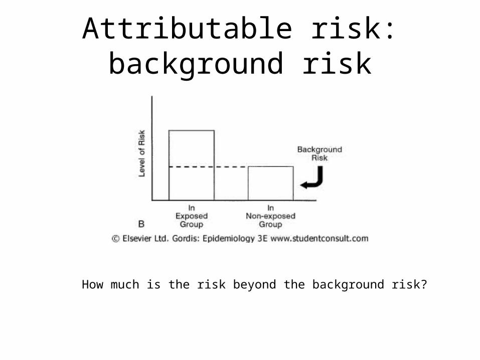
Attributable risk: background risk

How much is the risk beyond the background risk?

Attributable risk: risk due to exposure

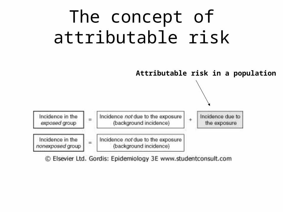
The concept of attributable risk

Attributable risk in a population

Number of deaths attributed to major causes, US, 1990

Attributable risk in public health and health policy

• Cause specific deaths data could lead to effective public policy

• AR could identify major health issues which could lead to implementation of screening and primary prevention programs

• In environmental health AR could help identify health problems that are attributed to environmental pollution

• AR greater than 50% has been used in defining the probability of “more likely than not” in legal claims of occupational and environmental problems

Comparison of relative risk and attributable risk

• Relative risk and odds ratio help understand the nature and the strength of association between exposure and disease development

• Attributable risk measures how much of the disease risk is attributable to a certain exposure

• Attributable risk also provides information on how much of the disease can be prevented if the exposure is avoided

• RR and OR are used in etiologic studies AR is used in public health and clinical practice

Cohort study review

Cohort studies inform us about the effect of exposureon disease development or etiological risk factors

Case control study review

Case control studies also address etiology and furthermoredetermine whether there is an excess risk or reduced riskof a certain disease with certain exposure or characteristic

The Hardest Thing About Case Control Studies is….

• Choosing the controls!

Problems in selection of controlsIn 1981, MacMahon and coworkers reported a case-control study of cancer of the pancreas.

The cases were patients with a histologically confirmed diagnosis of pancreatic cancer in 11 Boston and Rhode Island hospitals from 1974 to 1979.

Controls were selected from all patients who were hospitalized at the same time as the cases; and they were selected from other inpatients hospitalized by the attending physicians who had hospitalized the cases.

One finding in this study was an apparent dose-response relationship between coffee consumption and cancer of the pancreas, particularly in women

MacMahon et al: coffee consumption and risk of pancreatic cancer

Table 10-6. Distribution of Cases and Controls by Coffee-Drinking Habits and Estimates of Risk Ratios

    Coffee Consumption (Cups/Day)  

Sex Category 0 1-2 3-4 ≥5 Total

M No. of cases 9 94 53 60 216

  No. of controls 32 119 74 82 307

  Adjusted relative risk* 1.0 2.6 2.3 2.6 2.6

  95% Confidence interval - 1.2-5.5 1.0-5.3 1.2-5.8 1.2-5.4

F No. of cases 11 59 53 28 151

  No. of controls 56 152 80 48 336

  Adjusted relative risk* 1.0 1.6 3.3 3.1 2.3

  95% Confidence interval - 0.8-3.4 1.6-7.0 1.4-7.0 1.2-4.6

*Chi-square (Mantel extension) with equally spaced scores, adjusted over age in decades: 1.5 for men, 13.7 for women. Mantel-Haenszel estimates of risk ratios, adjusted over categories of age in decades. In all comparisons, the referent category was subjects who never drank coffee.From MacMahon B, Yen S, Trichopoulos D, et al: Coffee and cancer of the pancreas. N Engl J Med 304:630-633, 1981.

MacMohan et al: coffee consumption and smoking status

Table 10-7. Estimates of Relative Risk* of Cancer of the Pancreas Associated With Use of Coffee and Cigarettes

  Coffee Drinking (Cups/Day)  

Cigarette Smoking Status 0 1-2 ≥3 Total†

Never smoked 1.0 2.1 3.1 1.0

Ex-smokers 1.3 4.0 3.0 1.3

Current smokers 1.2 2.2 4.6 1.2 (0.9-1.8)

Total* 1.0 1.8 (1.0-3.0) 2.7 (1.6-4.7)  

*The referent category is the group that uses neither cigarettes nor coffee. Estimates are adjusted for sex and age in decades.†Values are adjusted for the other variable, in addition to age and sex, and are expressed in relation to the lowest category of each variable. Values in parentheses are 95% confidence intervals of the adjusted estimates.From MacMahon B, Yen S, Trichopoulos D, et al: Coffee and cancer of the pancreas. N Engl J Med 304:630-633, 1981.

MacMohan et al: study design• Did patients with pancreatic cancer drank more coffee than

people without cancer of the pancreas in the same population• Cases – patients with cancer of the pancreas• Controls – patients with other diseases admitted by the same

physician• Cases consumed greater amounts of coffee and that the

controls consumed less amount but equivalent to that of the general population

• Case selection and coffee consumption is good– Coffee consumption was higher

• Control selection and coffee consumption may not be optimal– Coffee consumption was lower

Coffee consumption among cases and controls

What is Smoking here?

Coffee Drinking Pancreatic Cancer

Smoking

Problems with selection of controls

• Controls are:– Similar to the cases (gastroenterology clinic)– Not representative of the general population

• Because of gastroenterology problems the controls may have reduced their coffee consumption

• They have altered their lifestyle• They may have altered their dietary habits• Reanalysis showed non significant increased risk• Hsieh et al repeated this study without support to the

original hypothesis

How Do We Reduce The Chances of Poor Choice of Controls?

• Matching

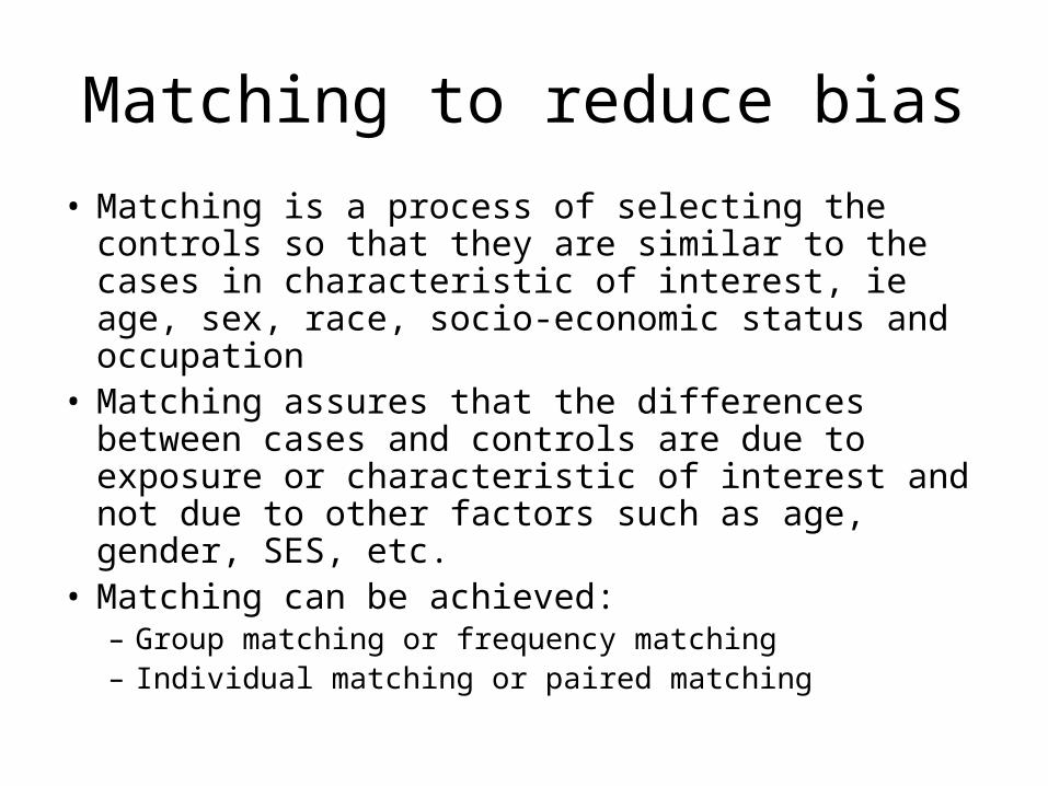
Matching to reduce bias

• Matching is a process of selecting the controls so that they are similar to the cases in characteristic of interest, ie age, sex, race, socio-economic status and occupation

• Matching assures that the differences between cases and controls are due to exposure or characteristic of interest and not due to other factors such as age, gender, SES, etc.

• Matching can be achieved:– Group matching or frequency matching– Individual matching or paired matching

Types of matching design• ________ matching or frequency matching

– Proportion of controls with certain characteristics is identical to the proportion of cases

– i.e. 25% of cases are black and 25% of controls are black– i.e. 50% of cases are women over 65 and 50% of controls

are women over 65 years of age• _________ matching or paired matching

– For each case a control is selected, who is similar to the case except for the specific variable of interest

– i.e. if the case is 45 years old female then the control will be 45±2 years old female

– i.e. if the case has completed university education then the control will also have competed university education

group

individual

Problems with matching

• Problems with matching:– Practical problems

• Matching is difficult and becomes cumbersome with each variable to be matched

– Conceptual problems• Matching for a given variable excludes that variable from being a

risk factor• Selection of a wrong variable for matching could produce

erroneous results and wrong conclusions

– Unplanned matching• Cases and controls may be matched without being known that the

cases are controls are matched for a variable

Recall problems in case control study

• Recall is invariably used in epidemiology in the process of collecting data from the research subjects

• Examples of recall– When was the last time you had sore throat?– What types of pesticides have you used on your vegetable

patch during the past ten years?– List all the jobs you have had in your lifetime?

• Types of recall problems– Limitation in recall– Recall bias

Types of recall problems

• Limitation in recall occurs when the research subject does not have the information that is requested– Lilienfield and Graham’s study of women with cervical

cancer based on the hypothesis that sexual intercourse with an uncircumcised men increase the risk of cervical cancer

– Men were asked on the status of their circumcision– Men were then examined by a physician to determine the

nature of their circumcision– In spite of this there is considerable differences of opinion

on the nature and degree of circumcision i.e the amount of foreskin left

Reported and observed data for circumcision in men

Table 10-8. Comparison of Patients' Statements With Examination Findings Concerning Circumcision Status, Roswell Park Memorial Institute, Buffalo, New York

  Patients' Statements Regarding Circumcision

  Yes No

Examination Finding

No. % No. %

Circumcised 37 66.1 47 34.6

Not circumcised 19 33.9 89 65.4

Total 56 100.0 136 100.0

Adapted from Lilienfeld AM, Graham S: Validity of determining circumcision status by questionnaire as related to epidemiologic studies of cancer of the cervix. J Natl Cancer Inst 21:713-720, 1958.

Types of recall problems

• Recall bias occurs when the research subject knowingly or unknowingly is biased in associating the characteristic or exposure to disease outcome– Mothers were interviewed post partum on probable events

during gestation that could have effected the birth outcome– Mothers with a baby with a defect is more likely to identify

some event that may be associated with the birth outcome– Whereas mother with a normal baby is less likely to identify

any event even though she may had one during her gestation

Effect of recall bias in a hypothetical studyTable 10-9. Example of Artificial Association Resulting From Recall Bias: A Study of Maternal Infections

During Pregnancy and Congenital Malformations

 

Cases (With Congenital

Malformations)

Controls (Without Congenital

Malformations)

Assume that:

True incidence of infection (%)

15 15

Infections recalled (%)

60 10

Result will be:

Infection rate as ascertained by interview (%)

9.0 1.5

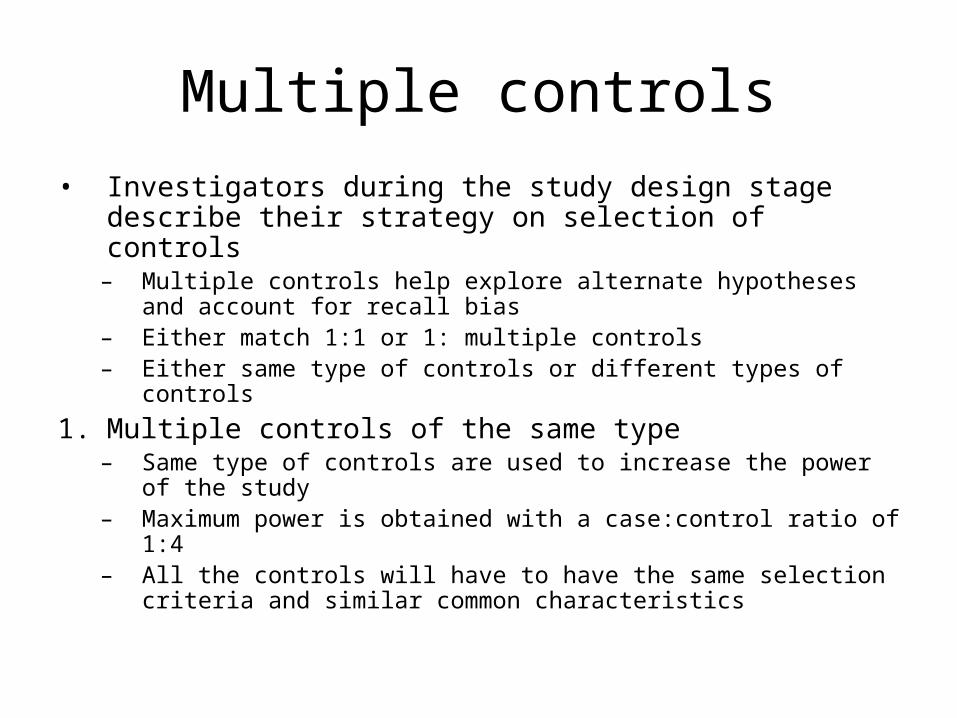
Multiple controls• Investigators during the study design stage describe their

strategy on selection of controls– Multiple controls help explore alternate hypotheses and account for

recall bias– Either match 1:1 or 1: multiple controls– Either same type of controls or different types of controls

1. Multiple controls of the same type– Same type of controls are used to increase the power of the study– Maximum power is obtained with a case:control ratio of 1:4– All the controls will have to have the same selection criteria and

similar common characteristics

Types of controls2. Multiple controls of different types

– Different types of controls are used to identify a gold standard or determine the bias of another set of controls and improve the validity of the study

– i.e first control could be selected from among the hospital patients– and the second control could be selected from the neighbourhood

or random digit dialling – If there is difference in the first and second controls than the better

control will be the reference control or the gold standard– Gold et al (1979) in the study on brain tumors in children identify

two controls• Children with no cancer (normal controls)• Children with other types of cancer (cancer controls)

Study design from Gold et al (1979)

Did mothers of children with brain cancers have more prenatal radiation exposure than control mothers?

Rationale for using two controls

First possibility

Rationale for using two controls

Second possibility

Case control studies• Case control studies are:

– Less expensive– Quicker to conduct and have a shorter duration– Good in establishing causal relationship between exposure

and disease– Used in establishing etiology of a disease– Ideal when the disease that is investigated is rare– Manageable because of the smaller number of research

subjects– Types of case control studies

• Nested case control study• Cross sectional study

Let’s say….

• You take a given population and follow them forward in time to see which ones develop a certain disease and which ones don’t…

• What kind of design is this?

Now let’s say….

• Everytime a case is identified who gets the disease, you select someone who doesn’t have it, and define the second person as the “control” for the first person (the “case”)

• After following this cohort for some time, you will have collected a group of “cases” and a group of “controls”

• Then you check their medical histories to see what their exposures were

• What kind of design is this?

Nested case control study

• Nested case control study is a hybrid design in which case control study is nested in a cohort study

Benefits of a nested case controls study

• Baseline data eliminates recall bias• Any changes in biological characteristics can

be reliably associated with the exposure• More economical to conduct

– Do not have to analyse all the samples collected from all the research subjects

– Only the samples from cases and controls are analysed

Risk estimation

• Absolute risk• Relative risk• Odds ratio• Interpretation of odds ratio

Absolute risk

• _____________ is the incidence of a disease in a population:– It indicates the magnitude of the risk in a group of

people with certain exposures– It does not take into account the risk in non-

exposed people– It does not indicate whether the exposure is

associated with increased risk of the disease

Risk estimation in case control and cohort studies

• Case control and cohort studies examine the relationship between exposure and disease development– Case control study: the focus is on the strength of this

association– Cohort study: how much bigger is the risk of developing

the disease in the exposed compared to the unexposed– The answer is in the relative risk

Relative risk• _____________ is defined as the probability of an event

(developing of a disease) occurring in exposed population compared to probability of the event in unexposed population or the ratio of these two events

• Ratio of the risk of disease in exposed individuals to the risk of disease in unexposed individuals

Interpretation of relative risk

• No evidence of increased risk• Positive risk• Negative risk

If RR = 1 Risk in exposed equal to risk in non-exposed (no association)

If RR > 1 Risk in exposed greater than risk in non-exposed (positive association; possibly causal)

If RR < 1 Risk in exposed less than risk in non-exposed (negative association; possibly protective)

But what about “2”?

Calculation of relative risk in a cohort study

Table 11-5. Risk Calculations in a Cohort Study

    Then Follow to See Whether    

   Disease

DevelopsDisease Does Not

Develop TotalsIncidence Rates of

Disease

First Select

Exposed a b a + b

Not exposed

c d c + d

 

Odds ratio (relative odds)

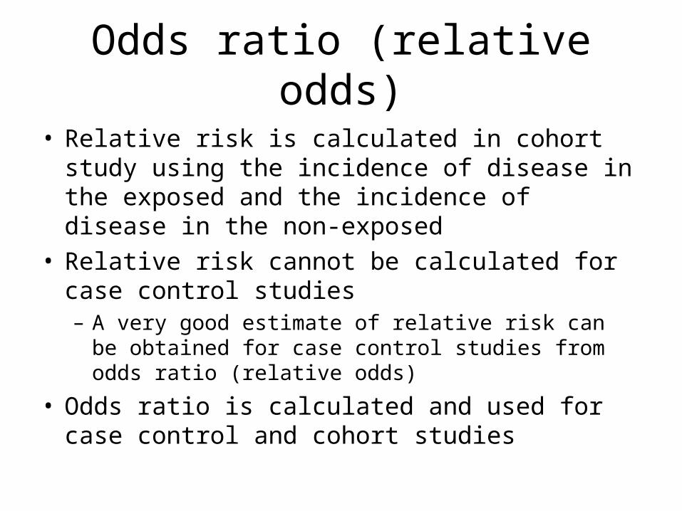
• Relative risk is calculated in cohort study using the incidence of disease in the exposed and the incidence of disease in the non-exposed

• Relative risk cannot be calculated for case control studies– A very good estimate of relative risk can be obtained for

case control studies from odds ratio (relative odds)

• Odds ratio is calculated and used for case control and cohort studies

The concept of odds• The odds of an event can be defined as the ratio of

the number of ways the event can occur to the number of ways the event cannot occur

• Suppose the probability of a horse winning a race is 60%, then the probability of the same horse loosing the race is 40% (100-60).

• Consequently the odds of winning the race is:= probability that the horse wins the race / probability that the horse looses the race= 60 / 40 = 1.5= P / (1-P)

Odds ratio

• Probability of winning 60%• Odds of winning 1.5

• Probability of loosing 40%

• Incidence rate• Attack rate• Risk of disease development

following exposure• Risk of disease development

without exposure

The odds ratio is a way of comparing whether the probability of a certain event is the same for two groups.

An odds ratio of 1 implies that the event is equally likely in both groups. An odds ratio greater than one implies that the event is more likely in the first group. An odds ratio less than one implies that the event is less likely in the first group.

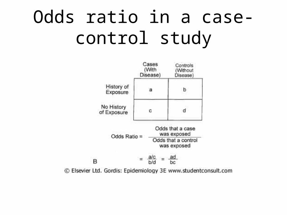
Odds ratio in a case-control study

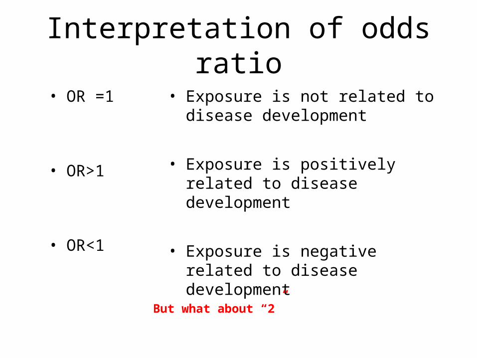
Interpretation of odds ratio

• OR =1

• OR>1

• OR<1

• Exposure is not related to disease development

• Exposure is positively related to disease development

• Exposure is negative related to disease development

But what about “2”

Odds ratio and relative risk• Case control studies permit calculation of odds ratio• Cohort studies permit calculation of odds ratio and

relative risk• Odds ratio can provide good approximation of

relative risk in a population– When cases are good representatives, with regard to the

history of exposure, of all people with the disease in the population from which cases are drawn

– When controls are good representatives, with regard to the history of exposure, of all people without the disease in the population from which controls are drawn

– When disease being studied does not offer frequently

Relative risk and odds ratio for an infrequent disease

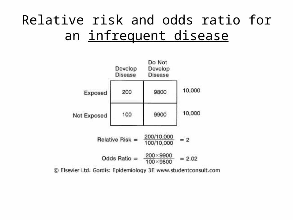
Relative risk and odds ratio for an infrequent disease

Relative risk and odds ratio for a frequent disease

Relative risk and odds ratio for a frequent disease

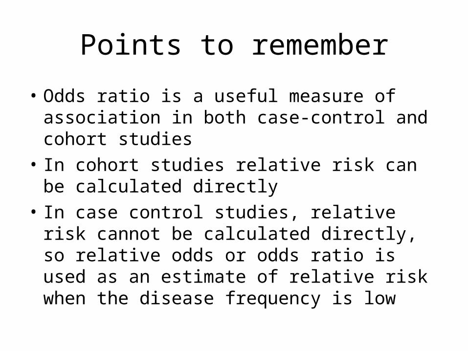
Points to remember

• Odds ratio is a useful measure of association in both case-control and cohort studies

• In cohort studies relative risk can be calculated directly

• In case control studies, relative risk cannot be calculated directly, so relative odds or odds ratio is used as an estimate of relative risk when the disease frequency is low

Briefly…

• You may have heard the term “Attack Rate”– Just a special kind of cumulative incidence rate,

computed during an epidemic or outbreak– Whereas the denominator for cumulative

incidence rate is the average size of the population ,

– The denominator for attack rate is the size of the population at the start of the outbreak or epidemic

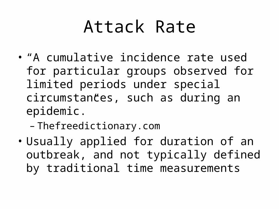
Attack Rate

• “A cumulative incidence rate used for particular groups observed for limited periods under special circumstances, such as during an epidemic.”– Thefreedictionary.com

• Usually applied for duration of an outbreak, and not typically defined by traditional time measurements

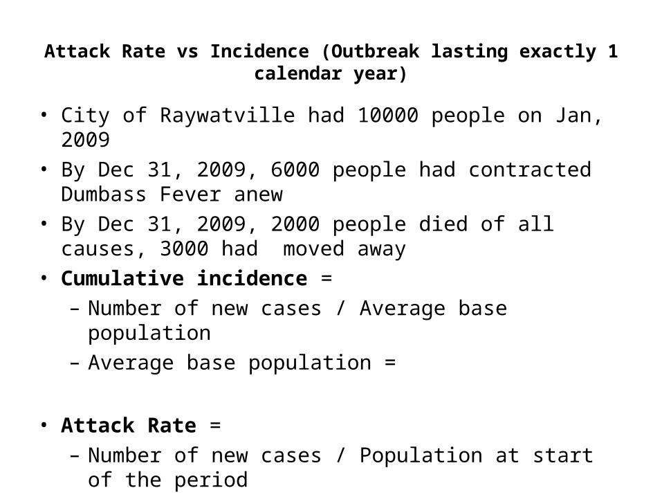
Attack Rate vs Incidence (Outbreak lasting exactly 1 calendar year)

• City of Raywatville had 10000 people on Jan, 2009• By Dec 31, 2009, 6000 people had contracted Dumbass Fever

anew• By Dec 31, 2009, 2000 people died of all causes, 3000 had

moved away• Cumulative incidence =

– Number of new cases / Average base population– Average base population =

• Attack Rate =– Number of new cases / Population at start of the period

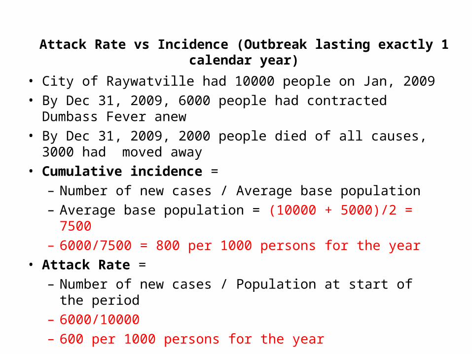
• City of Raywatville had 10000 people on Jan, 2009• By Dec 31, 2009, 6000 people had contracted Dumbass Fever

anew• By Dec 31, 2009, 2000 people died of all causes, 3000 had

moved away• Cumulative incidence =

– Number of new cases / Average base population– Average base population = (10000 + 5000)/2 = 7500– 6000/7500 = 800 per 1000 persons for the year

• Attack Rate =– Number of new cases / Population at start of the period– 6000/10000– 600 per 1000 persons for the year

Attack Rate vs Incidence (Outbreak lasting exactly 1 calendar year)

Why Employ the Attack Rate?

• Usually used in outbreak investigation, usually for foodborne illnesses

• Traditionally, when computing attack rate, we do not include people not at risk in the denominator– Eg, attack rate of measles would not include those

who’ve had the disease previously

Secondary Attack Rate

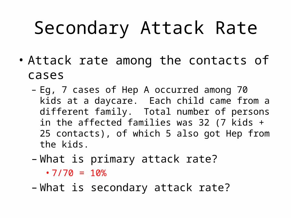
• Attack rate among the contacts of cases– Eg, 7 cases of Hep A occurred among 70 kids at a daycare.

Each child came from a different family. Total number of persons in the affected families was 32 (7 kids + 25 contacts), of which 5 also got Hep from the kids.

– What is primary attack rate?

– What is secondary attack rate?

Secondary Attack Rate

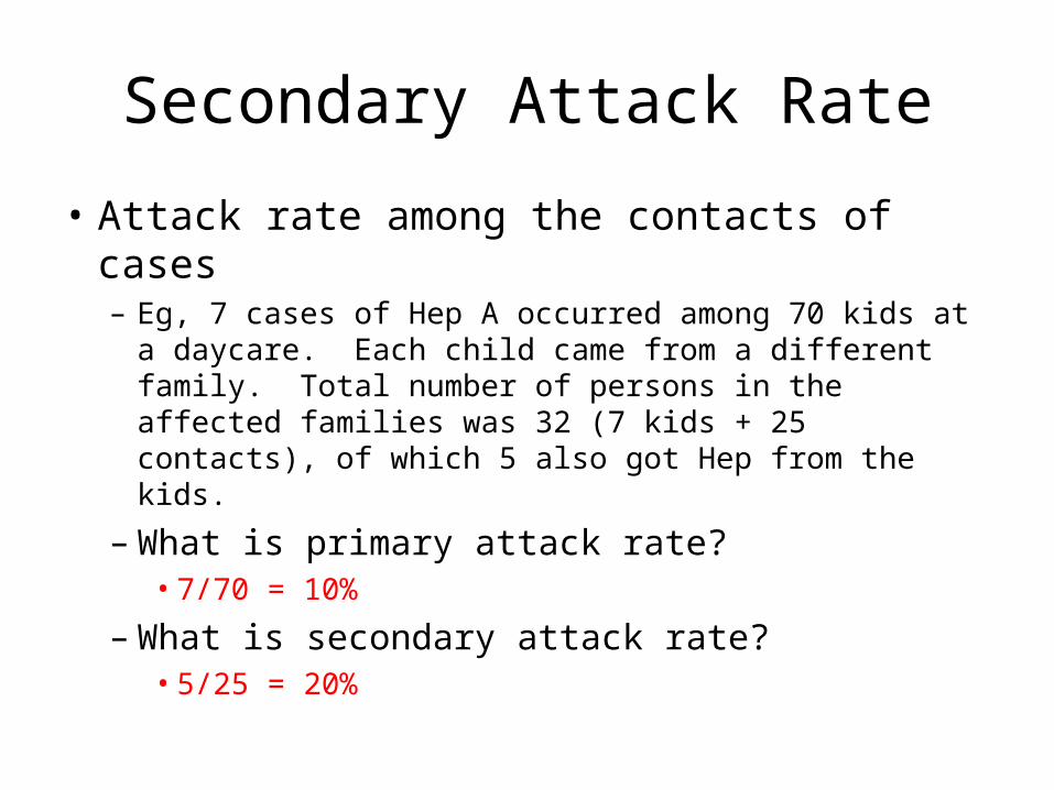
• Attack rate among the contacts of cases– Eg, 7 cases of Hep A occurred among 70 kids at a daycare.

Each child came from a different family. Total number of persons in the affected families was 32 (7 kids + 25 contacts), of which 5 also got Hep from the kids.

– What is primary attack rate?• 7/70 = 10%

– What is secondary attack rate?

Secondary Attack Rate

• Attack rate among the contacts of cases– Eg, 7 cases of Hep A occurred among 70 kids at a daycare.

Each child came from a different family. Total number of persons in the affected families was 32 (7 kids + 25 contacts), of which 5 also got Hep from the kids.

– What is primary attack rate?• 7/70 = 10%

– What is secondary attack rate?• 5/25 = 20%

MEASURE NUMERATOR DENOMINATOR

Incidence Rate #new cases during time period

Average pop during time interval

Attack Rate #new cases during epidemic period

Pop at the start of the epidemic interval

Sec Attack Rate #new cases among contacts during epidemic period

Size of contact pop at risk

Point Prevalence

#known cases at a given point in time

Estimated pop at the same point in time

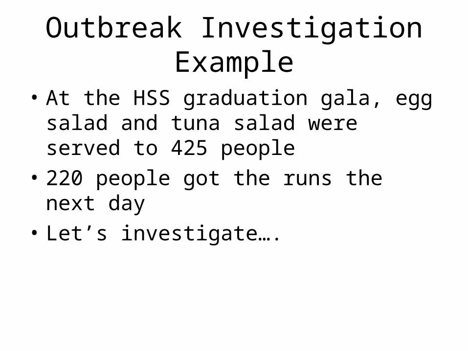
Outbreak Investigation Example

• At the HSS graduation gala, egg salad and tuna salad were served to 425 people

• 220 people got the runs the next day• Let’s investigate….

Ate tuna

Did not eat tuna

Ate egg salad

75 100

Did not eat egg salad

200 50

All students who attended

Ate tuna

Did not eat tuna

Ate egg salad

60 75

Did not eat egg salad

70 15

Those who got sick

What is the attack rate in persons who ate tuna but not the egg salad?

What is the attack rate in persons who ate egg salad only?

What is the attack rate in persons who ate both egg salad and tuna?

70/200 = 35%

75/100 = 75%

60/75 = 80%

Which food is most likely to be the culprit? Egg salad

STEPS FOR INVESTIGATING AN OUTBREAK12345678910

Determine the existence of an epidemicConfirm the diagnosisDefine a case and count casesOrient the data In terms of time, place and personDetermine who is at riskDetermine an hypothesis, and test it using statsCompare hypothesis with established factsPlan a more systematic studyPrepare a written reportExecute control and prevention measures

Slight variation here:

http://www.cdc.gov/excite/classroom/outbreak/steps.htm