WORKING PAPER SERIES

Michael J. Kottelenberg (Huron University College) Steven F. Lehrer (Queen's University, NYU-Shanghai and NBER)

How Skills and Parental Valuation of Education Influence Human Capital Acquisition and Early Labor Market Return to Human Capital in Canada

Winter 2019, WP #17

How Skills and Parental Valuation of EducationInfluence Human Capital Acquisition and Early Labor

Market Return to Human Capital in Canada

Michael J. KottelenbergHuron University College

Steven F. Lehrer∗

Queen’s University, NYU-Shanghai and NBER

February 2019

Abstract

Using the Youth in Transition Survey we estimate a Roy model with a three dimensionallatent factor structure to consider how parental valuation of education, cognitive skillsand non-cognitive skills influence endogenous schooling decisions and subsequent labourmarket outcomes in Canada. We find the effect of cognitive skills on adult incomesarises by increasing the likelihood of obtaining further education. Further, we findthat both non-cognitive skills and parental valuation for education play a larger rolein determining income at age 25 than cognitive skills. Last, our analysis uncoversstriking differences between men and women in several of the estimated relationships.Specifically, simulations of the estimated model illustrate that i) among the low skilled,women have much higher college graduation rates, ii) the age 25 earnings gradient byeither skill measure is much flatter for women, and iii) parental valuation of educationplays a larger role in influencing young women than men.

∗We thank seminar participants at the 2014 CLSRN/CEA Annual meetings, University of Calgary, NBERPublic Policies in Canada and the United States conference and the University of Calgary for helpful com-ments and suggestions. A special thanks to Ross Finnie and Stephen Childs for their help in the early stagesof this project. Kottelenberg and Lehrer also wish to thank EPRI and SSHRC for research support. Weare grateful to the Ontario Ministry of Training, Colleges and Universities for generous financial supportthrough the Ontario Human Capital Research and Innovation Fund and note that the views expressed inthe publication are the views of the Recipient and do not necessarily reflect those of the Ministry. The usualcaveats applies.

1

1 Introduction

Over the last decade, research by economists documenting both declining economic mobil-

ity (e.g. Chetty et al., 2014, Corak et al., 2014) and rising economic inequality (e.g. Saez

and Zucman, 2016, Autor et al., 2008) has captured the attention of policymakers and the

popular press. Within each literature, studies have also documented significant time-varying

gender differences in both how education influences labor market outcomes (e.g. Fortin et

al., 2015, Goldin et al., 2006) as well as how the effects of family and neighborhood charac-

teristics influence educational attainment and career prospects (e.g. Chetty and Hendren,

2018, Autor et al., forthcoming, Chetty et al., 2016). One of the primary challenges facing

researchers in these areas is that many of the candidate explanations for the observed hetero-

geneity are variables that are difficult to reliably measure using surveys, such as individual

skills or parental aspirations. In this paper, we use factor models as a means to flexibly

but parsimoniously model several of these latent candidate variables. We then subsequently

examine the role these candidate factors play in generating early adult outcomes, thereby

allowing us to connect and contribute to these two literatures.

Bridging these literatures is important since many traits including skills and preferences

are transmitted from parents to children. Parents not only make direct time and material

resource investments into their child’s human capital and skill production function, they also

instill levels of educational expectations in their children. While economists first formally

considered the role of parental investments in child development in Leibowitz (1974), there

have been relatively few studies of the role played by parental beliefs and expectations, in

part since they are difficult to reliably measure. Whether parental educational expectations

influence a child’s educational outcome has also attracted the attention of researchers in

both sociology and psychology, who have developed large literatures documenting a strong

positive association.1 Parents’ educational expectations serve as a major influence on chil-

dren’s expectations and in a review of the literature in psychology, Schneider and Stevenson

(1999) concluded, “One of the most important early predictors of social mobility is how

1 Recent contributions in psychology documenting how parents view education can influence their child’seducational attainment include studies using a U.S. nationally representative sample (Jacob and Linkow,2011) and is also found among high risk samples (Ou and Reynolds, 2008). Within the literature insociology, there is evidence that parents’ educational expectations matter for children’s educational at-tainment (e.g. Teachman, 1987; Wood et al., 2007) and can have long-term influences on children’s adultlife outcomes (e.g. Jacobs et al. 2006; Flouri and Hawkes 2008).

2

much schooling an adolescent expects to obtain”. One aim of this study is to isolate the

contribution of parents’ valuations of education at age 15—conditional on a child’s level of

skills at that age—on subsequent schooling decisions and early labor market outcomes.

While few studies in economics have explored the role of parental valuation of education,

a growing body of research surveyed in Heckman and Mosso (2014) has developed that

emphasizes the role of skills on life outcomes and the technology of skill formation. This

body of research has clearly established that skill is not only multidimensional in nature

(e.g. see Cunha and Heckman, 2008, Borghans et al., 2008) but also that skills develop in

a heterogeneous manner over the lifecycle (e.g. Hansen et al., 2003; Cunha et al., 2010;

Ding and Lehrer, 2014). Further, while a substantial body of research (e.g. Green and

Riddell, 2003; Hartigan and Wigdor, 1989; Murnane, et al., 2000; Heckman et al., 2006)

has shown that cognitive skills such as literacy and problem-solving matter, an emerging

body of evidence (e.g. Cunha and Heckman, 2008; Borghans et al., 2008; and Almlund et.

al., 2011, among others), suggests that social and emotional skills such as perseverance and

self-control are equally as important as cognitive skills in enhancing an individuals’ future

education and career prospects.

Evidence in the latter studies is derived primarily from the estimation of economic models

of skill development using longitudinal data collected in either the United States, South

Korea or England. These studies do not additionally consider the effects of parental valuation

of education on young adult outcomes. In this paper, using longitudinal data that tracks a

cohort of Canadians from age 15 through to age 25, we present the first empirical evidence

of the role of these three latent competencies that jointly influence schooling decisions and

subsequent labor market outcomes in Canada.2

Our empirical analysis builds on the economic framework developed by Willis and Rosen

(1979) who model self-selection into college and potential earnings within a traditional Roy

model. Our empirical approach offers two major advantages. First, we treat parental valua-

2 Foley et al. (2014) and Foley (forthcoming) also estimate a three-factor model to respectively understandhigh school dropout decision for males and the gender gap in university enrollment in Canada. Beyondthe different outcomes considered, the second estimation step in these papers includes a single choiceequation and does not consider potential outcomes. This distinction is important since these studies focuson understanding how observed and unobserved factors respectively relate to a specific decision, whereasour focus is to control for unobserved heterogeneity, thereby allowing for the simulation of accuratecounterfactuals of schooling and labor market outcomes. As discussed in detail in section 3, our studyalso differs in how the distribution of factors are identified and estimated.

3

tions of education and the two skill dimensions as a vector of low dimensional factors, rather

than using proxy variables to account for types of unobserved competencies. By using lin-

ear factor analysis methods to recover the distribution of three latent competencies, we can

more accurately capture a single parental valuation and multiple skill dimensions as well

as account for potential measurement errors in these latent competencies, while imposing

weaker assumptions on the data. Second, we explicitly model two sequential selection pro-

cesses,3 allowing us to identify all of the channels through which each competency measured

at earlier ages affects schooling and labor market outcomes in early adulthood. That is,

by considering the timing of these choices, we can separate out how different competencies

affect labor market outcomes into components explained by schooling and productivity.

We also contribute to the literature evaluating the labor market consequences of different

measures of skills by following the suggestion in Prada and Urzua (2017) and explore gender

differences.4 A growing literature not only documents gender differences in non-cognitive

skills at early ages (e.g. Cornwell et al., 2013) but also differences in parental behaviors

by child gender (e. g. Lundberg, 2005; Kottelenberg and Lehrer, 2018). Since gender

employment patterns suggest that occupational differences between men and women are a

persistent presence in North American labor markets, abilities may be rewarded differently

and in a manner that is consistent with observed occupational choices. Our analysis will

help develop an understanding of an economic mechanism behind the role of skills in the

labor market.

The first set of results is obtained from variance decompositions of the models used

to estimate the distribution of the latent factors. We find that cognitive skills explain

between 60-75% of the PISA test scores across subject areas. More striking is that responses

to questions related to the child’s perception of parent attitudes appears to capture the

lion’s share of variation in parental valuation of education. This finding is consistent with

evidence in psychology that children form their educational expectations largely in response

to parental inputs (e.g. Jacobs and Eccles, 2000; Schneider et al., 2010).

3 This modeling follows Heckman et al., (2006) and Urzua (2008), where individuals first decide whether toinvest in higher education, considering their predetermined competencies, the influence of both parentsand peers, as well as both skill and educational investments that may influence labor market outcomes.Second, workers select into jobs based on their competencies and their previous schooling choices.

4 To the best of our knowledge, only Prada and Urzua (2017) have previously estimated a three factormodel to understand how different dimensions of unobserved skills influence endogenous schooling andlabor market outcomes. Their analysis used a sample of white males in the United States.

4

The second set of results, obtained from simulations of the model, indicate that hetero-

geneity in the effects of each competency on both education and labor market outcomes along

gender lines is empirically important. Specifically, we observe that for girls, the probability

of self-reported tertiary education completion at age 25 is above 25% in every cognitive skill

decile. In addition, the gradient in college graduation across non-cognitive skill deciles is

quite flat for Canadian women. We find that in comparison to men, the parental valuation

for education has a larger influence on both women’s college degree completion. Women

with higher non-cognitive skills or parental valuation for education earn larger labor market

premiums. In contrast, for young men cognitive skills are found to play the largest role on

expected earnings, and their expected earnings decline with the parental factor. Given that

we uncover significant heterogeneity in the effects of each competency by gender, our results

highlight the trade-offs that policymakers face when developing policies that cultivate any

of these competencies.

While these differences are striking, our four remaining principal findings in the full

sample appear consistent with US evidence. First, we find that the average treatment effect

of university education in the full sample is positive. Second, non-cognitive skills play a

role in determining income at age 25 that is slightly larger than cognitive skills. Third,

accounting for the education decision is crucial to understand how cognitive skills affect age

25 income. The channel of increasing the likelihood of obtaining further education accounts

for roughly one-third of the effect of cognitive skills on income. In contrast, non-cognitive

skills influence age 25 income levels not only through the educational choice channel, but they

are additionally directly rewarded in the labor market. Fourth, simulations of the estimated

model show the cumulative effect of these two channels of influence for non-cognitive skills

are twice as large as that of cognitive skills. The effect of non-cognitive skills is slightly

smaller than the parental factor on income, but cognitive skills do play the largest role on

the decision to complete college.

This paper is structured as follows. Section 2 describes the data set we analyze. The

economic framework that underlies the econometric analysis is sketched in section 3, where

we additionally consider the conditions needed to identify the structural parameters of the

model. Our empirical results are presented and discussed in section 4. Simulations of the

model are undertaken to clearly illustrate the role played by the two dimensions of skill and

5

parental valuation of education on educational attainment and early labor market outcomes.

A final section draws the main conclusions.

2 Data

We use data from the Youth in Transition Survey (YITS-A) collected by Statistics Canada.

This study used a two-stage sampling frame to follow a nationally representative cohort of 15-

year olds. In the first stage, 1,187 schools were selected. From these schools, 29,867 students

were randomly selected in the second stage. Among these students, 29,330 participants

first completed both the OECD Performance for International Student Achievement (PISA)

reading test and the separate YITS survey questionnaire. In the first cycle, students, the

student’s principal, and either a parent or guardian who identified him or herself as ”most

knowledgeable” about the child completed a survey, providing additional and likely more

accurate measures of home and school inputs.5 Follow-up surveys were conducted with only

the students on a biennial basis until they reached 25 years of age.

This paper uses factor analysis methods to construct measures of different competencies

that applied econometricians do not directly observe including cognitive skills, non-cognitive

skills and parental valuation for education. Responses to three different questions in the

YITS-A survey are used to measure the parental factor. The questions include responses on

a four point scale of what is the highest level of education they hope their child completes.

Parents are then asked to use a four point scale to attach the importance they place on

their child getting education beyond high school. The scale runs from not important to

very important and is also used by the child to give their perspective of how important they

believe their parent(s) feel that they complete more education after high school.6

The YITS-A data contains measures of cognitive skills obtained from three domains of

the PISA test. While every student within the sample completed the reading test, only half

of them wrote either the math or science test and a smaller minority completed all three

tests. In addition there are a battery of questions to measure multiple dimensions of non-

5 Approximately, 13 percent of the parents did not complete the parental survey which was conducted overthe phone.

6 For children in two-parent households, we took the maximum of the child’s response associated with eachguardian.

6

cognitive skills. In this paper, we use information collected from three scales. Self-esteem

is measured using the 10-item Rosenberg (1965) scale that measure’s one general feelings of

self-worth. A self-efficacy scale adapted from Pintrich and Groot (1990) measures perceived

competence and confidence in academic performance. Last, a sense of mastery scale provides

an appraisal of the individual’s sense of broader control and consists of questions related to

one’s ability to do just about anything they set their minds to.

Since the YITS-A surveys the child, parent and school principal, a rich set of controls

including demographics, parental education and family income are available. Besides stan-

dard conditioning variables, we use information on the expectation of one’s peers at age

15, family structure, family income and wealth,7 immigration status, and whether parent’s

have set money aside for future education. The definitions of these variables are provided in

appendix A.

Throughout our analysis, we control for geographic differences since there is substantial

regional heterogeneity in both labor markets and how higher education is delivered. In

particular, the province of Quebec has a special system where students only attend secondary

school to the equivalent of grade 11.8 Canada has distinct regional labor markets (e.g.,

Atlantic Canada, Quebec, Ontario, the Prairies, and British Columbia) that differ sharply

by both policies of sub-national governments and industry compositions that can experience

pronounced boom and bust cycles (e.g. Morrisette et al. 2015).9

As with many longitudinal studies, there is substantial attrition within the YITS-A.

While Statistics Canada does provide sampling weights to accommodate several of these

features, given that we focus on parental valuation of education, cognitive and non-cognitive

skills, our primary analysis restricts the sample to include those individuals who completed all

7 Income is derived from wages/salaries, self-employment, and governmental transfers and social assistance.In contrast wealth is a proxy calculated by the availability of a suite of material goods including dishwasher,cell-phones, television sets, cars, computers, number of bathrooms in the primary residence and whetherthe student has both her own bedroom and access to the internet at home.

8 Following high schools students in Quebec can attend a two year College d’enseignement general et profes-sionnel (CEGEP), which further prepares one for a university degree. As such, those attending universityin Quebec normally can complete university in three years, compared to four years in the rest of Canada.Students interested in a technical degree in Quebec, generally register in a three year CEGEP program.

9 Since we have data for a single cohort and the geographic identifiers in the data are coarse, there is verylittle within geographic unit variation that can be exploited to shed light on the differences in labor marketconditions within regions. In appendix E, however, we do examine the impact of including provincial leveldata on unemployment and labour force participation rates in our model and find no significant differencesin our main results.

7

three PISA tests, have complete income and education data until age 25 and have a parental

survey. In addition, we dropped a handful of subjects that were either i) home-schooled

or ii) attending a school on an Indian reserve at age 15, or iii) that are no longer residing

in Canada at age 25. All of these restrictions combine to substantially reduce the number

of observations available and the final sample consists of 1607 individuals. To examine the

robustness of our findings, we used imputation methods to fill some of the missing covariates

allowing us to conduct additional analyses with a sample of 6,181 individuals.10

Table 1 presents summary statistics for different samples of the YITS data. The first

column presents information on all individuals measured in the first wave. The second column

presents information on the subsample that completed two of the PISA tests. The third

column presents information on our imputation sample and last column provides summary

statistics on those with complete records. The first two panels of the table present the

standardized test scores which show that this estimation sample is more skilled than the

full sample with non-cognitive scores roughly .15 standard deviation higher and cognitive

scores averaging between .3 and .5 standard deviations above the reference group.11 Notice

that individuals who completed at least two PISA tests outperform the reference group,

indicating that there is likely some sample selection in who completes the tests.

Further, the estimation sample is relatively affluent as indicated by the wealth index in

the third panel of Table 1. Nearly 75% of parents in this sample have set some money aside

for their child’s post-secondary education. Last by age 25, the last panel shows that over

50% of this sample has received a university degree. In summary, this sample selection leads

to a group of young Canadians that are both more skilled and better-supported than the

general population.

3 Model

In an important paper, Willis and Rosen (1979) develop and estimate a model of the demand

for schooling that take account of heterogeneity in ability levels, tastes and the capacity to

10 The imputation procedure is described in appendix D. The findings in the main text are re-conducted withthis sample. We note the sample restrictions also lead to many observations being dropped in studiesusing U.S. data. For example, Prada and Urzua (2017) end up with 1022 individuals from an originalsample of 12,686.

11 Following Statistics Canada guidelines we report our summary statistics using the YITS-A survey weights.

8

finance schooling investments. The model assumes that high school or college education

prepares an individual for a position in one of two occupations and allows for the possibility

of comparative advantage. Similar to the Roy (1951) and Heckman and Sedlacek (1985)

models, the notion that individuals may have latent talents that are not directly applied

on their job is considered. The main challenge that empiricists face in this area is that the

latent factors are unobserved to the econometrician. We will follow an emerging body of

research that uses factor analysis methods to identify these factors and their distribution; as

an alternative to employing (noisy) proxy variables.

Briefly, this model closely follows Heckman et al. (2006) and involves three steps that are

important for the empirical strategy. First, we need to estimate the predetermined dimen-

sions of ability as well as the existing parental valuation of education when the child reaches

age 15. We assume that each child is endowed with a three dimensional competency vector

θ at conception. Competency may subsequently develop due to parental investments and

other environmental interactions that may interact with the child’s invariant genetic char-

acteristics. We use factor analysis methods to estimate a system of test score and parental

valuation equations designed to identify and recover the distribution of latent competen-

cies. With latent predetermined competencies we next consider estimating equations that

integrate over these distributions to focus on how skills and parental valuation of education

affect two decisions the child makes after age 15: whether to complete a university degree

and subsequently which sector of the economy to work in.

This timing of decision making is important since we will decompose the importance of

latent competencies in determining labor market outcomes in early adulthood, into com-

ponents explained by schooling and productivity. The structural parameters from these

estimated equations are then used to simulate outcomes given different levels of the three

competencies. Below, we expand on the three steps of the model, focusing on how identifi-

cation is obtained in each step and then outline the estimation strategy.12

12 This framework is similar to studies using US data including Urzua (2008) and Prada and Urzua (2017),which also build off identification results from Carneiro et al. (2003).

9

3.1 Latent Competencies

Since ability is multidimensional and difficult to measure precisely, a range of statistical

and psychometric techniques have been developed to measure these latent characteristics.

Intuitively, the idea underlying these techniques is that many test scores and questionnaires

in surveys are designed to measure a concept and as such can be viewed as noisy proxies

for domains of ability. For example, performance on either a reading or a math exam may

be a noisy proxy for latent intelligence. Since these proxies of latent ability are imperfect

and based on a noisy signal of an individual’s underlying abilities, and thus are subject to

measurement error. Similarly, proxies for parental beliefs about the value of education are

also challenging to reliably measure. A growing number of studies by economists have built

on insights in Kotlarski (1967) to develop methods to identify the underlying distribution of

latent competencies requiring at least three measures of noisy proxies.13

In the first step, we must assume the number of domains of latent competencies we wish

to identify and which elements of the YITS-A data provide a noisy signal of the competency

in question. We consider cognitive skills that will be identified by the latent factor associated

with three standardized tests (reading (T c0 ), mathematics (T c1 ), and science (T c2 ) from the

PISA test, as well as non-cognitive ability is governed by the latent factor associated with the

scales associated with self-efficacy (T nc0 ), a sense of mastery (T nc1 ), and self-esteem (T nc2 ).14

This factor can loosely be interpreted as confidence: confidence in one’s ability to influence

outcomes, in one’s ability to master material, and in one’s self-image. The final factor that

we interpret as parental valuation for education is associated with ordered responses to

parental questions related to the highest educational attainment they hope for their child

(T p0 ), importance of the child getting more education after high school (T p1 ), and the child’s

perspective of how much education after high school their parents wishes they compete (T p2 ).

Equations (1) - (3) describes a measurement system linking the test measures found in

the data, T , to both the unobserved competencies (or factors), θs, and the individual context,

13 See Carneiro et al. (2003) for further details. but in actually to identify f factors we only need 2f + 1test scores. In our analysis, we have an additional test score and noisy measure for parental valuation ofeducation.

14 Non-cognitive abilities are heterogeneous and difficult to reduce to one factor. While we could consideradditional domains of non-cognitive skills using other variables measured in the YITS-A, we focus on asingle non-cognitive factor to facilitate comparisions with the majority of U.S. studies that consideredonly a single non-cognitive domain.

10

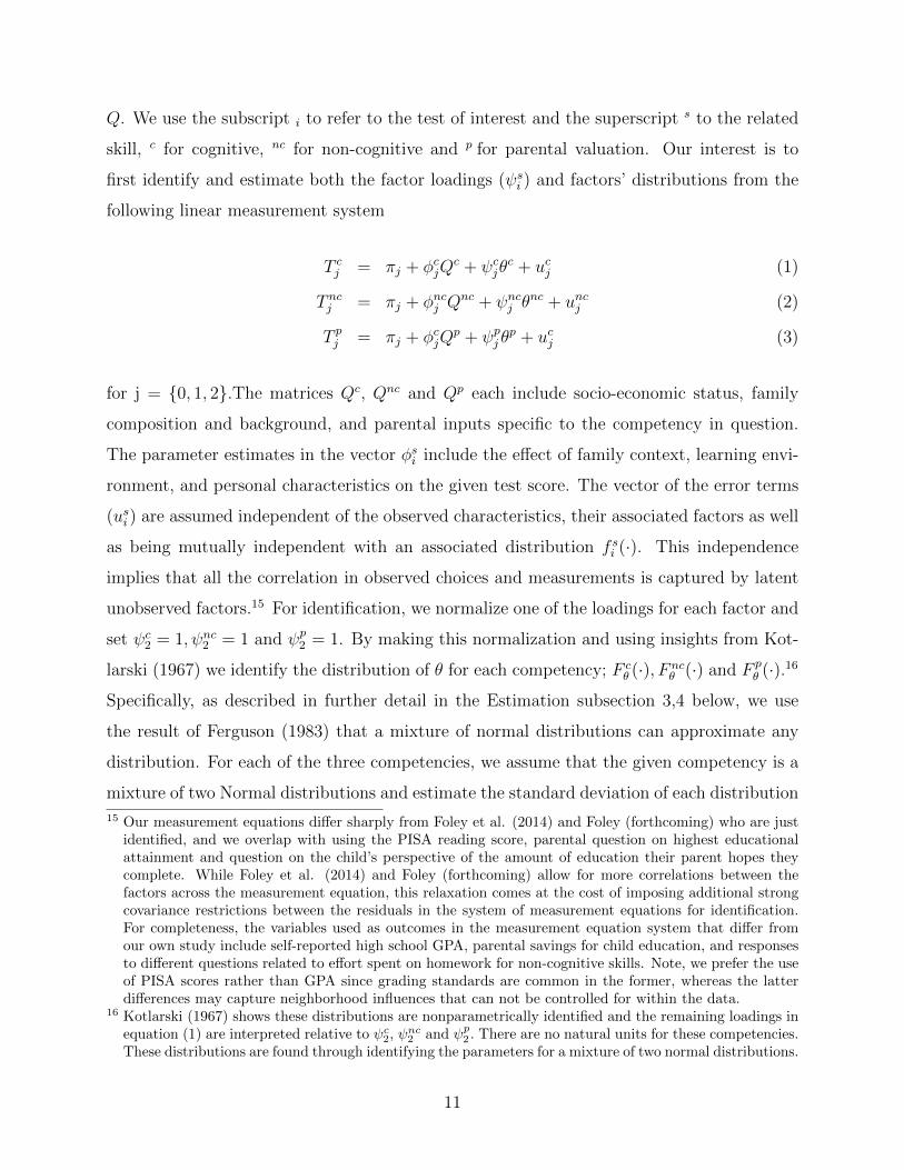
Q. We use the subscript i to refer to the test of interest and the superscript s to the related

skill, c for cognitive, nc for non-cognitive and p for parental valuation. Our interest is to

first identify and estimate both the factor loadings (ψsi ) and factors’ distributions from the

following linear measurement system

T cj = πj + φcjQc + ψcjθ

c + ucj (1)

T ncj = πj + φncj Qnc + ψncj θ

nc + uncj (2)

T pj = πj + φcjQp + ψpj θ

p + ucj (3)

for j = {0, 1, 2}.The matrices Qc, Qnc and Qp each include socio-economic status, family

composition and background, and parental inputs specific to the competency in question.

The parameter estimates in the vector φsi include the effect of family context, learning envi-

ronment, and personal characteristics on the given test score. The vector of the error terms

(usi ) are assumed independent of the observed characteristics, their associated factors as well

as being mutually independent with an associated distribution f si (·). This independence

implies that all the correlation in observed choices and measurements is captured by latent

unobserved factors.15 For identification, we normalize one of the loadings for each factor and

set ψc2 = 1, ψnc2 = 1 and ψp2 = 1. By making this normalization and using insights from Kot-

larski (1967) we identify the distribution of θ for each competency; F cθ (·), F nc

θ (·) and F pθ (·).16

Specifically, as described in further detail in the Estimation subsection 3,4 below, we use

the result of Ferguson (1983) that a mixture of normal distributions can approximate any

distribution. For each of the three competencies, we assume that the given competency is a

mixture of two Normal distributions and estimate the standard deviation of each distribution

15 Our measurement equations differ sharply from Foley et al. (2014) and Foley (forthcoming) who are justidentified, and we overlap with using the PISA reading score, parental question on highest educationalattainment and question on the child’s perspective of the amount of education their parent hopes theycomplete. While Foley et al. (2014) and Foley (forthcoming) allow for more correlations between thefactors across the measurement equation, this relaxation comes at the cost of imposing additional strongcovariance restrictions between the residuals in the system of measurement equations for identification.For completeness, the variables used as outcomes in the measurement equation system that differ fromour own study include self-reported high school GPA, parental savings for child education, and responsesto different questions related to effort spent on homework for non-cognitive skills. Note, we prefer the useof PISA scores rather than GPA since grading standards are common in the former, whereas the latterdifferences may capture neighborhood influences that can not be controlled for within the data.

16 Kotlarski (1967) shows these distributions are nonparametrically identified and the remaining loadings inequation (1) are interpreted relative to ψc

2, ψnc2 and ψp

2 . There are no natural units for these competencies.These distributions are found through identifying the parameters for a mixture of two normal distributions.

11

as well as both the mean shift for one of these distributions and the mixture probability.

In the above linear measurement system, we follow Prada and Urzua (2017), Heckman

et al. (2006), among others and treat each skill and parental valuation for education inde-

pendently. We are imposing an upper triangular assumption on the measurement system,

that requires each of the factors to be mutually independent. This assumption may appear

strong since one could postulate that performance on the PISA tests is a function of both

cognitive and non-cognitive skills or vice versa. We investigate the sensitivity of our con-

clusions to relaxing the assumption of mutual independence in appendix D. Specifically, we

no longer assume that each test measure is a ”pure” measure of specific competency, but do

maintain the assumption for a small subset of test measures. The results are quite similar to

results obtained when mutual independence is assumed.17 As such, we are comfortable with

a measurement system where each measure has a dedicated factor which ensures the factor

loadings can be interpreted to scale.18

3.2 The Education Decision

We now model the impact of skills and parental valuation for education at age 15 on a subse-

quent educational investment decision: whether to complete a university degree or not. This

decision is based on expected returns given their levels of latent competencies that has been

accumulated by age 15 and their potential earnings for each education level. We assume

that latent competencies are unobserved by the econometrician but the individual has full

information about his/her competencies, as well as knowledge of their returns. We do not

consider the exact timing of the decisions and assume that individuals make optimal educa-

17 This robustness exercise uses a two factor set-up and relaxes assumptions made in the formulation ofequation (1). We considered a variant that allowed the scales to reflect both cognitive and non-cognitiveskill factor but the non-cognitive skill factor was excluded in the equations used to measure the PISAsubject test scores. While the main results appear robust to a two factor model that treats each testmeasure to be a ”pure” measure of a specific factor, there were large computational costs associated withrelaxing these assumptions. As such, we follow Prada and Urzua (2017) and exclude the cognitive skillfactor as a determinant of any non-cognitive test score and vice versa.

18 This interpretation comes from normalizing one loading per factor to equal 1. As discussed in AppendixD, relaxing mutual independence does allow for a richer interpretation of variance decompositions oftest measures, but the factor loading themselves become more challenging to interpret. It should alsobe pointed out that the assumption of independence among the idiosyncratic errors in the measurementsystem is equally strong as restricting test measures to be a function of a single factor. While Williams(2018) provides new identification results involving reduced rank restrictions for the setting of correlatederrors across test measures for a single factor, we did not consider this extension.

12

tional choices when deciding between completing and not completing a university degree by

the age of 25. Each individual chooses the education level and sector of employment that

provides the highest payoff among the feasible choice set.

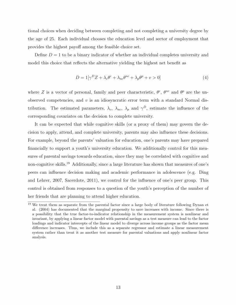
Define D = 1 to be a binary indicator of whether an individual completes university and

model this choice that reflects the alternative yielding the highest net benefit as

D = 1[γDZ + λcθc + λncθ

nc + λpθp + v > 0] (4)

where Z is a vector of personal, family and peer characteristic, θc, θnc and θp are the un-

observed competencies, and v is an idiosyncratic error term with a standard Normal dis-

tribution. The estimated parameters, λc, λnc, λp and γD, estimate the influence of the

corresponding covariates on the decision to complete university.

It can be expected that while cognitive skills (or a proxy of them) may govern the de-

cision to apply, attend, and complete university, parents may also influence these decisions.

For example, beyond the parents’ valuation for education, one’s parents may have prepared

financially to support a youth’s university education. We additionally control for this mea-

sures of parental savings towards education, since they may be correlated with cognitive and

non-cognitive skills.19 Additionally, since a large literature has shown that measures of one’s

peers can influence decision making and academic performance in adolescence (e.g. Ding

and Lehrer, 2007, Sacerdote, 2011), we control for the influence of one’s peer group. This

control is obtained from responses to a question of the youth’s perception of the number of

her friends that are planning to attend higher education.

19 We treat them as separate from the parental factor since a large body of literature following Dynan etal. (2004) has documented that the marginal propensity to save increases with income. Since there isa possibility that the true factor-to-indicator relationship in the measurement system is nonlinear andinvariant, by applying a linear factor model with parental savings as a test measure can lead to the factorloadings and indicator intercepts of the linear model to diverge across income groups as the factor meandifference increases. Thus, we include this as a separate regressor and estimate a linear measurementsystem rather than treat it as another test measure for parental valuations and apply nonlinear factoranalysis.

13

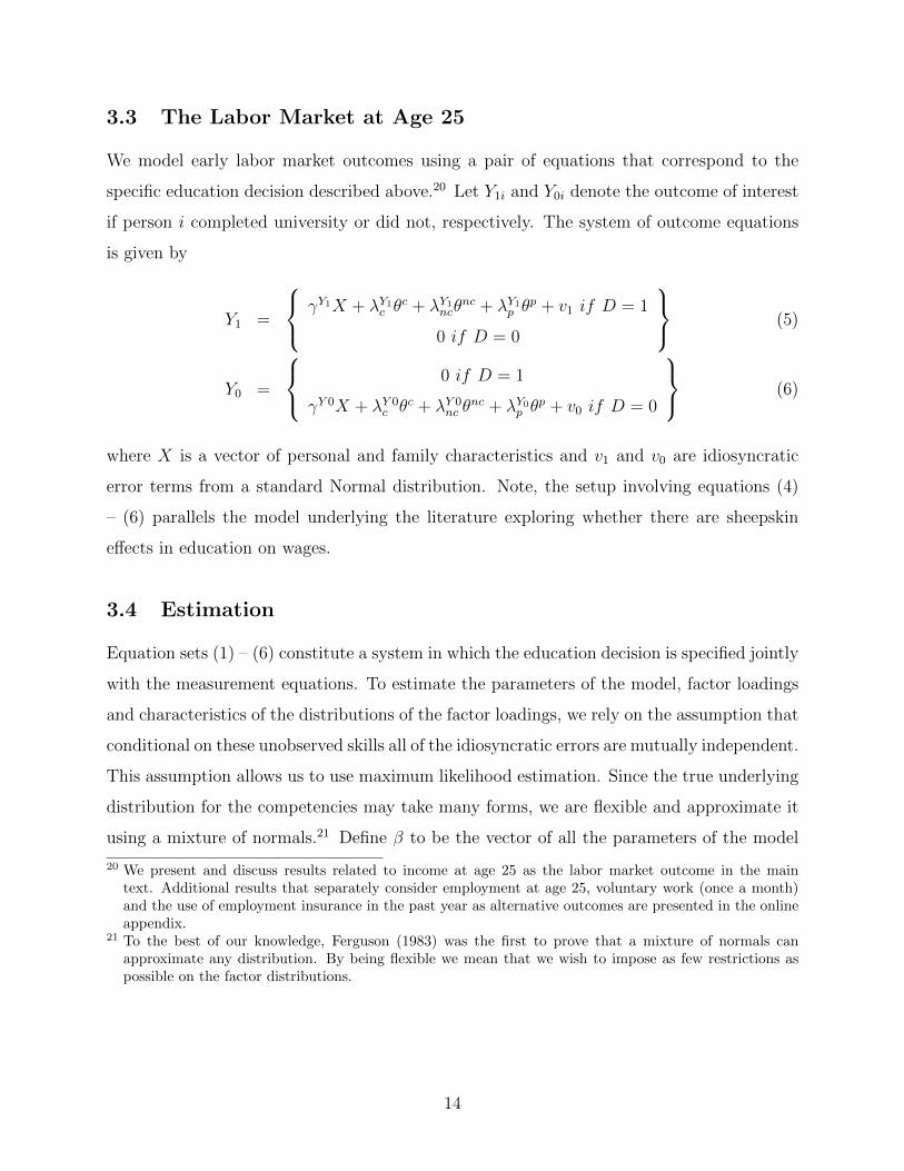
3.3 The Labor Market at Age 25

We model early labor market outcomes using a pair of equations that correspond to the

specific education decision described above.20 Let Y1i and Y0i denote the outcome of interest

if person i completed university or did not, respectively. The system of outcome equations

is given by

Y1 =

γY1X + λY1c θc + λY1ncθ

nc + λY1p θp + v1 if D = 1

0 if D = 0

(5)

Y0 =

0 if D = 1

γY 0X + λY 0c θc + λY 0

nc θnc + λY0p θ

p + v0 if D = 0

(6)

where X is a vector of personal and family characteristics and v1 and v0 are idiosyncratic

error terms from a standard Normal distribution. Note, the setup involving equations (4)

– (6) parallels the model underlying the literature exploring whether there are sheepskin

effects in education on wages.

3.4 Estimation

Equation sets (1) – (6) constitute a system in which the education decision is specified jointly

with the measurement equations. To estimate the parameters of the model, factor loadings

and characteristics of the distributions of the factor loadings, we rely on the assumption that

conditional on these unobserved skills all of the idiosyncratic errors are mutually independent.

This assumption allows us to use maximum likelihood estimation. Since the true underlying

distribution for the competencies may take many forms, we are flexible and approximate it

using a mixture of normals.21 Define β to be the vector of all the parameters of the model

20 We present and discuss results related to income at age 25 as the labor market outcome in the maintext. Additional results that separately consider employment at age 25, voluntary work (once a month)and the use of employment insurance in the past year as alternative outcomes are presented in the onlineappendix.

21 To the best of our knowledge, Ferguson (1983) was the first to prove that a mixture of normals canapproximate any distribution. By being flexible we mean that we wish to impose as few restrictions aspossible on the factor distributions.

14

and W = {Q,Z,X}, the likelihood is

L(β|W ) =n∏i=1

∫∫∫f(Di, Yi, Ti|Qi, Zi, Xi, θ

c, θnc, θp)dF cθ (·)dF nc

θ (·)dF pθ (·). (7)

To estimate equation (7) we integrate over the distribution of the three factors using Gauss-

Hermite quadrature for numerical integration.22 In the next section, we present and discuss

estimates of this model to consider the impact of unobserved competencies on educational

choices and income at age 25.23

This estimation treats the model as static and it should be explicitly stated does make

strong assumptions on how much adolescents know about their skill levels and parental

valuation for education. The education decision is evaluated only when the individual is

25 years old and does not consider the exact timing of the schooling decision. Since this

modeling does not either impose strict guidelines on either preferences or what is the full

content of the information set, Heckman et al. (2016b) point out thereby ensuring that

agents may not be aware of all factors that could influence how they value more schooling

when they make this decision. This modeling does provide a clear advantage by allowing

individuals to regret their earlier irreversible decision to attend college, a feature consistent

with evidence from post-graduation surveys.24

4 Results

We begin by discussing the parameter estimates, factor loadings and factor distributions ob-

tained from maximum likelihood estimation of equation (7). For space considerations, Table

2 presents estimates of how each of the unobserved latent competencies (θc, θnc and θp) and

other covariates influence each of the test measures in the model described in equations (1)–

(3). For space considerations we only include analysis from the full sample.25 Recall, for

22 The distributions of the underlying factors are estimated separately from equation (7).23 Note, for estimation of the analysis presented in the online appendix which considers alternative outcomes

that are all given by discrete indicators, an individual’s contribution to the likelihood function is simplythe product of normal CDF evaluations when we condition on the factors.

24 Similarly, behavioral models where individuals have self-serving beliefs or are over-confident about theirabilities will also generate individuals continuing their education despite the ex-post benefiit being nega-tive.

25 We observe differences between the genders in the effect of parental valuation on educational aspiration forchildren, where the estimated magnitude for young women is roughly 50% larger in magnitude. Similarly,

15

identification purposes, one loading for each unobserved competency is set to one and the

remaining loadings must be interpreted in relation to the loading set as the numeraire. In

examining the role of the covariates from equations (1)-(3) we find several interesting gender

differences in the estimated relationships, where perhaps unsurprisingly girls score higher on

the PISA reading test, whereas boys score higher in math. While we do not find a significant

gender difference in science,26 females perform significantly worse than the males on two of

the non-cognitive test measures.27

The estimates in Table 2 reveal striking regional differences in each cognitive measure.

Ontario, the base group, has ceteris parabus lower cognitive test scores than both the western

Canadian provinces and Quebec. On non-cognitive measures, the Atlantic provinces have

significantly lower sense of mastery and self-esteem scores than Ontario. Further, family

wealth rather than income wealth plays a larger role on performance in math and on both

parental aspirations and on parental importance of post-secondary education. Parental edu-

cation levels are highly correlated to the cognitive test scores measures, even when controlling

for the cognitive skill.

Holding the cognitive skill factor constant, youth from non-traditional families perform

significantly better on the science tests. Not surprisingly those from non-traditional families

fare worse on measures of their non-cognitive ability and this is likely related to changes in

their self-perception relating to their experiences in transitioning between different family

structures.28 Perhaps, these children face similar parental aspirations and parents rank the

importance of future education similarly. As a whole, these results suggest that the situation

we observe a slightly smaller effect of the non-cognitive factor on both self-efficacy and sense of masteryfor girls relative to boys.

26 Using a novel assessment based on the PISA that was administered in different regions of urban China,Ding et al (2018) demonstrate that gender gaps in scientific performance depend heavily on which domainsof scientific intelligence are being tested. The PISA science score is obtained by asking questions related tothe concept of scientific literacy from four domains -across context, knowledge, attitude and competencies.

27 We are referring to a non-cognitive skill that could be capturing conscientiousness, which matters fora wider spectrum of job complexity (Barrick and Mount 1991). We would expect that higher levels ofsocio-emotional abilities are more important for some occupations requiring low-order cognitive skills,especially in the service sector (Bowles et al. 2001). Occupational choices are driven by personalitycompetencies such as being a caring or a direct person in adolescence (Borghans et al. 2008). Individualspartly select occupations that correspond to their orientations. competencies related to grit (persistenceand motivation for long-term goals) seems to be essential for success no matter the occupation throughtheir effect on education achievements (Duckworth et al. 2007).

28 Note that this does not indicate lower levels of non-cognitive skill for those in non-traditional families,though this may be the case, but rather lower scores on the non-cognitive tests given a level of the latentnon-cognitive skill.

16

at home can be important to determining measures such as grades and thus educational

pathways.

To shed further light on the relative importance of each dimension of unobserved com-

petency in explaining test measures used as outcomes (T ), Figure 1 presents the variance

decomposition of the measurement system. The results present the contribution of observed

covariates, latent competencies and and unobservables as determinants of the variance of

each test measure. The contribution of observed variables to the variance of any of the nine

test measures never exceed 8% and not surprisingly play virtually no role for the child’s

impression of the importance their parents place on post secondary education. Interestingly

between 60-80% of the variance in PISA test scores can be explained by our cognitive fac-

tor.29 The cognitive skill factor appears to explain more of the variation on the reading test,

the subject where performance in the underlying data exhibits less variation than underlying

either the PISA math or science test score.

Perhaps, the most striking result in Figure 1 is that much of the variance in parental val-

uation for education arises from the single measure of the child’s perception of the parent’s

valuation. This result implies that at age 15, the child’s perception of their parents impor-

tance is a fairly accurate predictor for the true parental valuation for education. The variance

decomposition illustrates the large size of the unexplained component for the additional two

test measures used to obtain the parental factor.

Figure 2 presents estimates of the distribution of each competency for each group by

educational decision and they appear to be quite different from the distribution of the un-

derlying test measures. For each competency, there is substantial overlap in the distribution

across education groups and Kolmogrov-Smirnov tests reject the assumption of the distri-

bution of skills being equal across these groups. The distribution of both the cognitive skill

and parental factor exhibits more variation for college graduates than the corresponding

distribution of non-graduates.

Table 3 presents the estimates of λcv, λncv , λ

pv and γ from equation (4), providing evidence

on the importance of cognitive and non-cognitive skills as well as the parental valuation

29 We are grateful to an anonymous reviewer for suggesting this analysis. In appendix D, we estimate richermodels for the measurement system that allow for some correlation and test measures to be a functionof two competencies such as the self-esteem score being a function of cognitive and non-cognitive skills.Even with richer models, we still find the explanatory power of the non-cognitive factor remains similarto estimates presented in figure 1.

17

factor on the decision to complete university. In the first column, we present results for

the full sample and the gender subsamples appear in the third and fourth column. The

second column presents results for the larger imputed sample. There are few differences in

the magnitude and statistical significance of estimates the full and imputed sample and each

competency enters the decision in a highly significant manner. There are several prominent

gender differences where we observe that the effect of non-cognitive skills is more than twice

as large for boys and the effect of the parental valuation for education competency is roughly

47% larger in magnitude for girls. In section 4.1, we provide a more intuitive understanding

of the role of each competency using a simulation of the model.

Several other results in Table 3 are consistent with the North American literature on

attending higher education. Females are much more likely than males to complete university,

holding other factors constant. Consistent with Belley et al. (2014), in the non-imputed

samples, family income and wealth are found to not significantly influence the completion of

university in Canada. We find that a measure of whether parents have put money aside for

post-secondary education plays a large role, even after conditioning on the parental valuation

for education factor. These savings reflect a reduction of the opportunity cost of education

and the results are suggestive of being more influential than current levels of family income

or wealth.

Our results also suggest that peers play a significant role in determining educational

attainment that is approximately twice as large for young men. While this variable is sta-

tistically significant, additional analyses presented in Appendix E shows that it has a very

small influence and that all of the results are robust to the exclusion of the peer measure.

There are also interesting gender differences in the effects of immigrant status and geographic

variables. Holding all else constant, women from the Atlantic provinces are much more likely

to go to university than men. In contrast, we find a significant reduction of females com-

pleting universities in Quebec relative to Ontario. Last, we find that the negative impact of

immigrant status on university completion is driven by men.

Tables 4 and 5 respectively present estimates of the parameters λs0, λs1, β0, and β1 from

Equations 5 and 6 for income and employment at age 25 conditional on educational attain-

ment. We continue to present results for four samples and the column headings of D = 1

and D = 0 refer to those who have completed and not completed a university degree respec-

18

tively. While each competency played a large role on the decision to complete university,

the majority of the effects of each competency on labor market outcomes are statistically

insignificant.

The results in this table show that cognitive skills significantly improve employment

rates amongst non-university graduates. The benefits of earning a higher income or higher

likelihood of having a job from possessing higher cognitive skills operate mainly through the

educational channel. This effect of cognitive skills on labor market outcomes is driven by

young men, who are penalized by employers for not having this credential. While university

graduates of both genders observe a positive gradient of the non-cognitive skill measure on

income, it is not statistically significant when we also control for the parental valuation of

education.30 The parental valuation for education factor significantly boosts salaries and

employment at age 25, an effect that is driven by the subsample of women. Last, a puzzling

finding that non-cognitive skills significantly decrease the odds of employment for women

with a college degree are employed at age 25. When contrasting these estimates to those

presented in the appendix C and D for a two factor model of cognitive and non-cognitive

skills, we can conclude that ignoring the parental valuation for education suggests a much

larger role for non-cognitive skills.

4.1 Evidence from Simulation of the Model

Simulation methods facilitate our understanding of the size and significance of the estimated

parameters discussed above. To conduct simulations, we first randomly draw an individual

and use their full set of regressors from the population. These individuals are paired with

random draws from each of the three distributions of the latent competencies, and the distri-

bution of each parametrized error term. Using the parameter estimates for the appropriate

sample, we can then explore the effects of both skills and parental valuation of education on

the outcomes of interest that are traced across individual contexts and through university

completion decisions. These simulations are presented in figures 3 and 4, which examine

how the university completion and income vary across levels of competency respectively.

The rows of each figure focus on a single competency and the columns of each figure present

30 Note, for those without a university degree, we find a gender difference in the sign of the estimated effectof non-cognitive skills on income, but the effects are statistically insignificant.

19

results for the full sample and each gender subsample. Throughout, this section, we ensure

that within subgroup, the deciles of skills are placed on a comparable scale.

The top row of figure 3 presents the probability of completing a university degree for each

decile of the cognitive skill distribution. Not surprisingly, for each sample the probability

of completing a degree increases dramatically with cognitive ability. At almost every skill

decile, college completion rates for men are roughly 10% lower than for women. In the lowest

deciles of the cognitive skill distribution, college completion rates for women always exceed

25%, whereas graduation rates are very low for young men with low cognitive skills.

The second row of figure 3 documents a positive gradient between non-cognitive skills

and the likelihood of university completion. The gradient for non-cognitive skills has a more

gradual incline than the gradient for cognitive skills. We continue to find gender differences

in the gradient and college completion rates for young men fall below rates for young women.

Last, there is limited heterogeneity in the completion rates across deciles of non-cognitive

skills for women.

While the gradient for college completion in either cognitive or non-cognitive skill is

steeper for men then women, the reverse occurs across the distribution of parental valuation

for education. The bottom row of figure 3 illustrates a positive gradient only among young

women. Further, at every decile of parental valuation for education, the college completion

rate for women is higher than at any and all deciles of the distribution for men. In contrast,

figure 4 shows a positive gradient for women at every decile of parental valuation for education

on income and a corresponding flat gradient for men. Income for females moves from roughly

$20,000 to $32,000 across the full distribution of the factor, whereas men’s income remains

effectively unchanged. However, the labor market income for women at any decile of this

competency is lower than at any and all deciles of the corresponding distribution for men.

Examining the panels in the top two rows of figure 4, we obverse a steep gradient for

non-cognitive skills on earnings for young women. Earnings climb from $22,000 to nearly

$31,000 across the deciles. However, even at the highest decile of non-cognitive skills, women

on average earn less than a man at any decile of the non-cognitive skill distribution. Sim-

ilarly, young women on average earn similar amounts at each decile of the cognitive skill

distribution. The gender gap appears quite large at roughly $12,000 at each decile of the

cognitive factor.

20

The interpretation of many of these gender gaps diminish once we condition on university

completion. Figure 5 illustrates the simulation results corresponding to two incomes at age 25

and estimated confidence intervals graphed across deciles of each competency.31 The dashed

line and dark blue shaded line respectively represent individual who did not complete college

and graduates. Across the panels presented in the first column of Figure 5, we observe fairly

flat gradients on income for the full sample for each competency. Across each competency,

we observe positive gradients for the full sample among university graduates. The positive

slopes for the cognitive and parental valuations are driven by a single gender. We observe

that only earnings among university graduated males increase across deciles of the cognitive

skill distribution moving from $27,000 to $40,000. There is a similarly large impact on female

graduates from the parental valuation factor; earnings nearly double moving from $20,000 at

the lowest decile to $35,000 at the highest decile. Both the male and female income gradients

are positive across the non-cognitive skill deciles with more moderate changes in earnings.

In contrast, we observe that annual earnings of young men who did not complete college

fall at higher levels of both cognitive and non-cognitive skills. These drops are more mild

at roughly $3,500 from 1st to 10th decile. Surprisingly, we also find that female college

graduates earn lower incomes at higher deciles of the cognitive skill distribution. For men,

the confidence intervals for income of men between graduates and non-graduates do not

overlap at the bottom and top deciles. For women, we observe that the 95% confidence

intervals do not overlap for all three competencies at virtually every decile, highlighting a

greater role for education.

Due to their multidimensional nature, cognitive and non-cognitive skills are rewarded

in the labor market according to their combinations (e.g. Urzua (2008), Prada and Urzua

(2017)). Figure 6 presents a new set of panels containing three dimensional graphs that

explores how the average simulated outcome varies across the two competency distributions

when evaluated. The most striking results appear in the third column for young women. The

top row of figure 6 presents combinations of the cognitive and non-cognitive factor, where

31 For completeness, we conduct the same analysis corresponding to other outcomes measured at age 25.In appendix figures B.1 and B.2 we observe that both being employed and use of employment insurancedo not appear to be affected by either skills. In appendix figure C.4d, we find that as the levels of bothskills increase so too does the likelihood that an individual engages in volunteering. We find that theslope across the cognitive skill dimension is steeper, which is somewhat surprising given the dimension ofnon-cognitive skill that we are likely capturing. However, the role of skills on volunteering are small inmagnitude and likely lack economic significance.

21

we observe a positive gradient for the non-cognitive factor at every decile of the cognitive

factor for young women.32 Similarly, in the middle row of figure 6 we observe the incline

of the gradient in the parental factor exists at each cognitive skill decile. This gradient

steepens across the deciles of the cognitive skills; the effect moving across the parenting

factor distribution is $4,000 at the lowest decile and $15,000 at the highest. The bottom

row of figure 6 illustrates the relationship between the non-cognitive and parental factor

and suggests that young womens’ earnings increase across both dimensions and at similar

rates. Taken together, these results illustrate that earnings rise at all higher combinations of

the non-cognitive skill and parental factors, but are generally flat across the cognitive skill

dimension for Canadian women.33

The second column of figure 6 presents the corresponding results for boys. For boys,

the picture is quite flat indicating absences of gradients in one competency, conditional on

another. The results suggest that only among boys in the very top cognitive skill deciles,

do earnings rise across the non-cognitive skill deciles. Similarly, we find a positive gradient

for cognitive skills at fewer higher deciles of the non-cognitive distribution. Last, we observe

that the size of the cognitive skill gradient declines across the parental factor deciles. As a

whole, the majority of the relationships observed in the full sample arise from the subsample

of women.

The results of the simulation exercise are summarized in table 7. The panels summarizes

how a one standard deviation change in each competency affects outcomes in the model

and through which pathway. The estimates indicate that each competency increases em-

ployment and income in the full sample. Non-cognitive skills play a substantially larger role

on university completion for boys, whereas the parental factor has a 50% larger effect for

women. Both non-cognitive skills and the parental factor play a large role in influencing

early adult earnings, but the gender differences in the magnitude of these effects exhibit a

different pattern compared to employment. Women receive a much larger gain in expected

earnings from increases in both the parental factor and non-cognitive factor then men. Last,

cognitive skills only significantly increase age 25 income for young men.

32 We should note that the returns to skills differ across type of work and different reward of set of skillsacross occupational activities. For example, see Levine and Rubinstein (2013) and Hartog et al. (2010)for evidence on the skills necessary for success as an entrepreneur.

33 The sole exception is there being a slight rise in gradient of cognitive skills conditional on a woman alsobeing in the highest deciles of the parental factor.

22

The pathway through which each of these skills are rewarded in the labor market differ

sharply by gender. Women benefit from a small indirect effect of cognitive skills that operates

through their schooling decision on labor market income. This effect is completely offset by

a direct labor market reward to cognitive skills. Young men face a significant negative

gradient to their cognitive skills through the indirect channel, but do receive large direct

rewards. These results suggest that employers can more accurately ascertain cognitive skills

of boys and that they directly value increased confidence of girls that may arise either from

their non-cognitive or parental factor.

In the full sample, we find that on average, attending four-year college is associated

with higher average earnings. However, there is an important gender difference in the sign

of the average treatment effect (ATE). We find a negative effect for boys, which suggests

that they are correctly sorting to higher education. Whereas, consistent with the less steep

gradient of college completion by cognitive skills for young women, we find a positive ATE.

As a whole, the results suggest that the labor market return to each competency increases

only for women who complete university, explaining why the average treatment effect for the

untreated is only positive for young Canadian women. In summary, the simulations provide

strong evidence of the multiple, heterogeneous ways each competency influences education

and labor market outcomes in Canada.

4.2 Discussion of similarities and differences to evidence in US

Studies

Since our approach builds off studies using US data, we briefly contrast our findings to

these, recognizing the importance of the suggestion in Card and Freeman (1993) that ”small

differences” in policies and institutions including the market for higher education, have led

to differences in economic outcomes between Canada and the US. Results from empirical

studies are not only conditional to their methodology but also of their context including

the time period of data collection and make-up of the population covered by the sampling

frame. A number of studies use data from the NLSY-79 (e.g. Heckman et al. 2006, 2016a;

Prada and Urzua, 2017; and Urzua, 2008) to measure cognitive skills and dimensions of

non-cognitive through proxy variables and make use of a similar framework to explore the

23

impact of these skills. The NLSY-79 and YITS-A ask different questions which explains why

the metrics used in the factor model to capture the two latent cognitive skills differ across

studies.34 Further, as Humphires and Kosse (2017) point out the term non-cognitive skills is

used broadly in the labor economics literature and how this factor is constructed influences

what conclusions are reached about the role of non-cognitive skills in life outcomes.35

Despite these caveats certain commonalities exist in our findings and the US literature.

First, both cognitive and non-cognitive skills are found to influence education and early labor

market outcomes. Second, the effects of these skills on earnings is mediated by educational

attainment. However, we identify important gender differences in these relationships.

Several of the relative differences in our findings between our study and work using United

States data appear consistent with other pieces of evidence in the labor economics litera-

ture.36 The labor market returns to different dimensions of skills appear higher in the United

States relative to Canada is respectively consistent with the returns to a university degree

and comparable workplace skill reported in Bowlus and Robinson (2012) and Hanushek et

al. (2015). We also speculate that the finding of a higher university completion rate for

Canadian women with low cognitive skills may provide an explanation for why the wage gap

between male and female workers reported in Finnie et al. (2016) widens each year after

graduation at a larger rate in Canada than the United States.

One of the main contributions of this study is to estimate a model that allows for three

dimensions of unobserved heterogeneity including a factor that captures the parents’ per-

ception of education as an investment in future income earning capacity. Economists dating

34 For example, our Canadian evidence used PISA scores when estimating the cognitive skill factor, the USevidence estimates the latent cognitive skill factor from measures of mathematical knowledge, numericaloperations and coding speed that were collected before children left high school. In our analysis, we cancondition on variables such as number of siblings and immigrant status; whereas this information is to thebest of our knowledge not available in the NLSY-79; in which researchers control for disability status andreligion. This provides other reasons why caution must be taken when comparing results across studiesusing this framework.

35 As Heckman et al. (2006) state the selection of variables is motivated by what is available in the data.Specifically, they (on p. 429) write “we choose these measures because of their availability in the NLSY79.Ideally, it would be better to use a wider array of psychological measurements and ... to connect themwith more conventional measures of preference parameters in economics.”.

36 Cohort differences due to the timing of the data collection may also account for some of the differences inthe estimated patterns from the simulations. For example, simulations using the NLSY-79 report a muchlarger effect of cognitive skills on income then we found. This result may arise since the Canadian data wascollected on a later cohort that may have experienced the reversal in the demand for skills documentedin Beaudry et al. (2014, 2016).

24

back to Becker (1962) have developed models of investment in human capital that postu-

lates that the demand for education is driven by a measure capturing parental valuation for

education. As the variance decomposition of these parental valuations illustrate that they

are known to the child at age 15, it is not surprising to see that they are correlated to the

two other dimensions of unobserved skills. By comparing estimates of both a two-factor and

correlated two factor model which are presented in Appendices C and D, with those pre-

sented in the main text, allows us to understand how omitting the parental factor influences

our estimates.

Assuming the two skills factors in the model are a sufficient statistic for the stock of

all latent competencies at age 15, then how much parents value education beyond skill

investment. In each specification of the two factor models presented in Appendix D, we do

include the noisy test measures used to construct the parental factor. At first glance, the

set of results seem similar. However, differences emerge in the effect of cognitive ability on

the decision to attend a four-year college and earnings associated with the scenario of not

attending a four-year college. Specifically, a one unit increase in cognitive ability increases

the probability of attending college by 26.8 and 24.1 percent points in a three-factor model

and a two factor model respectively. In earnings regressions that include the parental factor,

the effect of non-cognitive ability for those not attending four-year college is less than one-

sixth of the effect estimated in a two-ability model. These results illustrate the differences

between our three-competency model and an alternative two-competency framework. While

many of the results are robust to the setup, for young women conclusions on the role of

non-cognitive ability and lack of steepness of the gradient of college attendance by cognitive

skill, mask the importance of omitting a dimension of parental heterogeneity.

Given the importance of the role of parents, we undertook additional analyses in Ap-

pendix D, where we reestimate the two-factor skill model for samples defined on the basis of

parental education. Motivating this investigation is that for policy audiences there is a need

to not just determine if there are potential deficits in skills for those who are disadvantaged,

but also to understand what are the potential benefits of any intervention that could foster

cognitive or non-cognitive skills. The results of the simulations reveal that at every skill

decile, children of less educated parents on average earn less than the corresponding children

of high educated parents; where a child of high educated parents has at least one parent with

25

some college education.37 Further, the results suggest that among young adults in the YITS,

completing a university degree does not significantly reduce the intergenerational effects of

family disadvantage.

5 Conclusion

Using the Youth in Transition Survey (YITS-A) we estimate a Roy model with a three

dimensional latent factor structure to consider how both cognitive and non-cognitive skills

as well as parental valuation for education influence endogenous schooling decisions and

subsequent labor market outcomes in Canada. Our analysis demonstrates that one third of

the effect of cognitive skills on adult incomes arises by increasing the likelihood of obtaining

further education. Conditional on the choice to complete a university degree, cognitive skills

are found to play a very small additional role in determining earnings at age 25. This finding

is driven by young women who do not achieve any benefit. In contrast, non-cognitive skills

not only indirectly influence adult income through the channel of educational choice, they

are directly rewarded in the labor market for both men and women. Young women also

achieve large benefits from parents having a higher value of education that operates through

both channels. Last, evidence from policy simulations suggest that there are trade-offs by

gender from developing policies that cultivate either different dimensions of non-cognitive

skills or the parental factor, relative to those that focus solely on cognitive skills.

Several of our findings differ from the existing evidence using data from the UK and the

US. First, the gradient in college completion among young Canadian women is less steep

and we speculate that the structure of the higher education markets likely play a large role

in ensuring access. Indeed, our additional analyses in the appendix find differences in college

completion rates across skill deciles for individuals raised in household that differ on the

basis of parental education. However, we find that at every skill decile individuals who have

at least one parent that is college educated earn $10,000 more a year on average than young

adults from families where neither parent persisted beyond high school.

Future work using Canadian data can follow Heckman et al. (2016a) by considering richer

37 Perhaps, most surprising is that on average the age 25 earnings of those with high skills and less educatedparents are not significantly different from the earnings of young adults in the lowest skill decile fromhouseholds where one parent has a higher level of education.

26

models of individual decision making and potentially examining how the type of higher

education people acquire influences career paths. In addition, Statistics Canada has now

linked participants in the YITS-A with federal tax records providing data that is unique in

its depth and containing more accurate data on annual income.38 This data can be used to

not only reduce measurement error in self-reported labor market earnings as well as errors

in any imputation procedure, but in combination with richer models should generate new

insights on the role of competencies influencing transitions of youth during this stage of the

life-cycle.

In summary, our analysis extends prior work that examined the role of multiple dimen-

sions of latent skills on schooling and labor market outcomes, by additionally incorporating

parental valuation for education in the set of an individual’s latent competencies. We find

that all three included factors influence the decision to complete college and each have addi-

tional multiple, heterogeneous, and independent effects on early labor market outcomes. We

identify striking gender differences in the main channels through which unobserved initial

competencies affect outcomes. We conclude by suggesting that this heterogeneity highlights

the challenges that policymakers face and cast doubt that one size fits all education policies

will be more effective than targeted policies in reducing economic inequality in the future.

38 Specifically, 18 years of the T1 Family File as well as other administrative databases have been linked byStatistics Canada to the majority of the YITS-A study participants.

27

References

Almlund, Mathilde, Angela L. Duckworth, James J. Heckman, and Tim D. Kautz. 2011.Personality psychology and economics. In The Handbook of The Economics of Education,ed. E. A. Hanushek, S. Machin and L. Woessmann, Amsterdam: Elsevier.

Autor, David H., David Figlio, Krzysztof Karbownik, Jeffrey Roth, and Melanie Wasser-man. Forthcoming. Family disadvantage and the gender gap in behavioral and educationaloutcomes. American Economic Journal: Applied Economics.

Autor, David H., Lawrence F. Katz, and Melissa S. Kearney. 2008. Trends in U.S. wageinequality: Re-assessing the revisionists, Review of Economics and Statistics 90 (2):300-323.

Barrick, Murray R., and Michael K. Mount. 1991. The big five personality dimensions andjob performance: A meta-analysis. Personnel Psychology 44 (1):1-26.

Beaudry, Paul, David A.Green, and Ben M. Sand. 2014. The declining fortunes of the youngsince 2000. The American Economic Review 104 (5): 381–386.

Beaudry, Paul, David A. Green, and Ben M. Sand. 2016. The great reversal in the demandfor skill and cognitive tasks. Journal of Labor Economics 34 (1): 199-247.

Becker, Gary S. 1962. Investment in human capital a theoretical analysis. Journal of Polit-ical Economy 70 (5): 9-49.

Belley, Philippe, Marc Frenette, and Lance Lochner. 2014. Post-secondary attendance byparental income in the US and Canada: Do financial aid policies explain the differences?Canadian Journal of Economics 47 (2): 664-696.

Borghans, Lex, Angela L. Duckworth, James J. Heckman, and Bas ter Weel. 2008. Theeconomics and psychology of personality competencies. Journal of Human Resources 43(4): 972-1059.

Bowles, Samuel, Herbert Gintis, and Melissa Osborne. 2001. The determinants of earnings:A behavioral approach. Journal of Economic Literature 39 (4): 1137–1176.

Bowlus, Audra, and Chris Robinson. 2012. Human capital prices, Productivity and growth.American Economic Review 102 (7): 3483-3515.

Card, David, and Richard B. Freeman. 1993. Introduction. In Small Differences That Mat-ter: Labor Markets and Income Maintenance in Canada and the United States, ed. D. Cardand R. B. Freeman. University of Chicago Press.

Carneiro, Pedro, Karsten Hansen, and James J. Heckman. 2003. Estimating distributionsof counterfactuals with an application to the returns to schooling and measurement of theeffect of uncertainty on schooling choice. International Economic Review 44 (2): 361-422.

Chetty, Raj, and Nathaniel Hendren. 2018. The impacts of neighborhoods on intergener-ational mobility I: Childhood exposure effects. Quarterly Journal of Economics 133 (3):1107-1162.

28

Chetty, Raj, Nathaniel Hendren, and Lawrence F. Katz. 2016. The effects of exposure tobetter neighborhoods on children: New evidence from the Moving to Opportunity experi-ment. American Economic Review 106 (4): 855-902.

Chetty, Raj, Nathaniel Hendren, Patrick Kline, and Emmanuel Saez. 2014. Where is theland of Opportunity? The geography of intergenerational mobility in the United States.Quarterly Journal of Economics 129 (4): 1553-1623.

Corak, Miles, Matthew J. Lindquist, and Bhaska Mazumder. 2014. A comparison of upwardand downward intergenerational mobility in Canada, Sweden and the United States. LabourEconomics 30 (2): 185-200.

Cornwell, Christopher, David B. Mustard, and Jessica Van Parys. 2013. Non-Cognitiveskills and the gender disparities in test scores and teacher assessments: Evidence fromprimary school. Journal of Human Resources 48 (1), 236-264.

Cunha, Flavio, and James J. Heckman. 2008. Formulating, identifying and estimating thetechnology of cognitive and noncognitive skill formation. Journal of Human Resources 43(4): 738-782.

Cunha, Flavio, James J. Heckman, and Susanne M. Schennach. 2010. ”Estimating thetechnology of cognitive and noncognitive skill formation,” Econometrica 78 (3): 883-931.

Ding, Weili, and Steven F. Lehrer. 2007. Do peers affect student achievement in China’ssecondary schools? Review of Economics and Statistics, 89 (2): 300-312.

Ding, Weili, and Steven F. Lehrer. 2014. Understanding the role of time-varying unobservedability heterogeneity in education production. Economics of Education Review 40 (1): 55-75.

Ding, Weili, Yipeng Tang, and Yongmei Hu. 2018. Closing the gender gap in science: Newevidence from urban China. Mimeo. Kingston, Ontario: Queen’s University.

Duckworth, Angela L., Christopher Peterson, Michael D. Matthews, and Dennis R. Kelly.2007. Grit: Perseverance and passion for long term goals. Journal of Personality and SocialPsychology 92 (6): 1087-1101.

Dynan, Karen E., Jonathan Skinner, and Stephen P. Zeldes. 2004. Do the rich save more?Journal of Political Economy 112 (2): 397-444.

Ferguson, Thomas S. (1983). Bayesian density estimation by mixtures of normal distri-butions. In Recent Advances in Statistics: Papers in Honor of Herman Chernoff on hisSixtieth Birthday, ed. H. Chernoff, M. H. Rizvi, J. S. Rustagi, and D. Siegmund. New York:Academic Press.

Finnie, Ross E., Kaveh. Afshar, Eda Bozkurt, Masashi Miyairi and Dejan Pavlic. 2016.Barista or better? New evidence on the earnings of post-secondary education graduates: Atax linkage approach. Mimeo. Ottawa, Ontario: EPRI, University of Ottawa.

29

Flouri, Eirini, and Denise Hawkes. 2008. Ambitious mothers–successful daughters: mothers’early expectations for children’s education and children’s earnings and sense of control inadult life. British Journal of Educational Psychology 78 (3):411-433.

Foley, Kelly, Giovanni Gallipoli and David A. Green. 2014. Ability, parental valuationsof education and the high school drop out decision. Journal of Human Resources 49 (4):906-944.

Foley, Kelly. Forthcoming. The gender gap in university enrollment: Do parents play a rolebeyond investing in skills? Canadian Journal of Economics.

Fortin, Nicole M., Philip Oreopoulos, and Shelley Phipps. 2015. Leaving boys behind:Gender disparities in high academic achievement. Journal of Human Resources 50 (3):549-579.

Goldin, Claudia, Lawrence F. Katz, and Ilyana Kuziemko. 2006. The homecoming of Amer-ican college women: The reversal of the college gender gap. Journal of Economic Perspec-tives,20 (4): 133-156.

Green, David A, and W Craig Riddell. 2003. Literacy and earnings: an investigation of theinteraction of cognitive and unobserved skills in earnings generation. Labour Economics 10(2): 165-184.

Hansen, Karsten, James J. Heckman, and Kathleen J. Mullen. 2003. The effect of schoolingand ability on achievement test scores. Journal of Econometrics 121 (1-2): 39-98.

Hanushek, Eric A., Guido Schwerdt, Simon Wiederhold, and Ludger Woessmann. 2015.Returns to skills around the world: Evidence from PIAAC. European Economic Review73(1): 103-130.

Hartigan, John A., and Alexandra K. Wigdor. 1989. Fairness in employment testing. Science245 (4913): 1-14.

Hartog, Joop, Mirjam Van Praag, and Justin Van Der Sluis. 2010. If you are so smart, whyaren’t you an entrepreneur? Returns to cognitive and social ability: Entrepreneurs versusemployees. Journal of Economics & Management Strategy 19 (4): 947-989.

Heckman, James J., and Guilherme Sedlacek. 1985. Heterogeneity, aggregation, and marketwage functions: An empirical model of self-selection in the labor market. Journal of PoliticalEconomy 93 (6): 1077-1125.

Heckman, James J., Jora Stixrud, and Sergio Urzua. 2006. The effects of cognitive andnoncognitive abilities on labor market outcomes and social behavior. Journal of Labor Eco-nomics 24 (3): 411-482.

Heckman, James J., and Stefano Mosso. 2014. The economics of human development andsocial mobility. Annual Review of Economics 6 (1): 689-733.

30

Heckman, James J., John E. Humphires, and Gregory Veramendi. 2016a. Returns to educa-tion: The causal effects of education on earnings, health and smoking. Journal of PoliticalEconomy 126 (S1): S197-S246.

Heckman, James J., John E. Humphries and Gregory Veramendi. 2016b. Dynamic treat-ment effects. Journal of Econometrics 191 (2): 276-292.

Humphires, John and Fabian Kosse. 2017. On the interpretation of non-cognitive skills –what is being measured and why it matters. Journal of Economic Behavior & Organization136: 174-185.

Jacob, Brian A. and Tamara W. Linkow. 2011. Educational expectations and attainment. InWhither opportunity: Rising inequality, schools, and children’s life chances, ed G. Duncanand R. J. Murnane. New York: Russell Sage Foundation.

Jacobs, Janis E., Jacqueline S. Eccles. 1992. The impact of mothers’ gender-role stereotypicbeliefs on mothers’ and children’s ability perceptions. Journal of Personality and SocialPsychology,63 (6): 932-944.

Jacobs, Janis E., Christina S. Chhin, and Martha M. Bleeker. 2006. Enduring links: Par-ents’ expectations and their young adult children’s gender-typed occupational choices. Ed-ucational Research and Evaluation 12 (4): 395-407.

Kotlarski, Ignacy I. 1967. On characterizing the gamma and the normal distribution. PacificJournal of Mathematics,20 (1): 69-76.

Kottelenberg, Michael J., and Steven F. Lehrer. 2018. Does Quebec’s subsidized child carepolicy give boys and girls an equal start? Canadian Journal of Economics 51 (2), 627-659.

Leibowitz, Arleen. 1974. Home Investments in Children. Journal of Political Economy 82(2): 111-131.

Levine, Ross and Yona Rubinstein. 2013. Smart and illicit: Who becomes an entrepreneurand does it pay? NBER Working Paper w19726, National Bureau of Economic Research,Cambridge, MA.

Lundberg, Shelly. 2005. Sons, daughters, and parental behavior. Oxford Review of EconomicPolicy 21 (3): 340-356.

Morissette, Rene, Ping C. W. Chan, and Yuqian Lu. 2015. Wages, youth employment, andschool enrollment: Recent evidence from increases in world oil prices. Journal of HumanResources 50 (1): 222-253.

Murnane, Richard J., John B. Willett, and John H. Tyler. 2000. Who benefits from obtain-ing a GED? Evidence from high school and beyond The Review of Economics and Statistics82 (1): 23-37.

Ou, Suh-Ruu, and Arthur J. Reynolds. 2008. Predictors of educational attainment in theChicago Longitudinal Study. School Psychology Quarterly 23 (2): 199-229.

31

Pintrich, Paul R., and Elisabeth V. De Groot. 1990. Motivational and self-regulated learningcomponents of classroom academic performance. Journal of Educational Psychology 82 (1):33-40.

Prada, Marıa F., and Sergio Urzua. 2017. One size does not fit all: Multiple dimensions ofability, college attendance and wages. Journal of Labor Economics 35 (4): 953-991.

Rosenberg, Manny. 1965. Society and the Adolescent Self-Image, Princeton: Princeton Uni-versity Press.

Roy, Andrew D. 1951. Some thoughts on the distribution of earnings. Oxford EconomicPapers 3 (2): 135-146.

Sacerdote, Bruce. 2011. Peer effects in education: how might they work, how big are theyand how much do we know thus far? In The Handbook of The Economics of Education, ed.E. A. Hanushek, S. Machin and L. Woessmann. Amsterdam: Elsevier.

Saez, Emmanuel and Gabriel Zucman. 2016. Wealth inequality in the United States since1913: Evidence from capitalized income tax data. The Quarterly Journal of Economics 131(2): 519-578.

Schneider, Barbara, Venessa Keesler and Larissa Morlock. 2010. The effects of family onchildren’s learning and socialization. In The nature of learning: Using research to inspirepractice, ed H. Dumont, D. Istance, and F. Benavides. Paris: OECD.

Schneider, Barbara, and David Stevenson. 1999. The ambitious generation: America’steenagers, motivated but directionless. New Haven: Yale University Press.

Teachman, Jay D. 1987. Family background, educational resources, and educational attain-ment. American Sociological Review 52 (4): 548–557.

Urzua, Sergio. 2008. Racial labor market gaps the role of abilities and schooling choices.Journal of Human Resources 43 (4): 919-971.

Williams, Benjamin. 2018. Identification of the linear factor model. Mimeo. Washington,DC: George Washington University.

Willis, Robert J. and Sherwin Rosen. 1979. Education and self-selection. Journal of PoliticalEconomy 87 (5): s7-s36.

Wood, Dana, Rachel Kaplan, and Vonnie McLoyd. 2007. Gender differences in the educa-tional expectations of urban, low-income African American youth: The role of parents andthe school. Journal of Youth and Adolescence 36 (4): 417-427.

32

Table 1: Mean and Standard Deviation of Key Variables

Complete Two PISA Imputation Three PISA ScoreVariables of Interest YITS Sample Scores Sample Sample Full Sample

Factor Test ScoresPISA Reading Score 0.102 0.330 0.401 0.529

(0.980) (0.917) (0.879) (1.047)PISA Math Score 0.079 0.308 0.381 0.331

(1.004) (0.936) (0.899) (0.876)PISA Science Score 0.090 0.321 0.388 0.429

(1.002) (0.943) (0.893) (0.889)Self-Efficacy 0.002 0.104 0.147 0.159

(1.000) (0.973) (0.960) (0.962)Sense of Mastery 0.002 0.090 0.120 0.135

(1.000) (0.985) (0.977) (0.994)Self-Esteem -0.005 0.089 0.125 0.151

(1.011) (1.001) (0.992) (0.949)Parent Educational Aspiration for Youth 3.748 3.797 3.831 3.845

(0.836) (0.789) (0.771) (0.764)Importance of Post-Secondary Education 3.854 3.854 3.874 3.891(Parent’s Answer) (0.424) (0.427) (0.382) (0.349)Importance of Post-Secondary Education 3.717 3.736 3.744 3.749(Youth’s Answer about Parents) (0.602) (0.571) (0.563) (0.542)

Individual and Family Characteristics, Age 15Female 0.501 0.508 0.514 0.496

(0.500) (0.500) (0.500) (0.500)Family Income (Thousands) 70.73 73.37 74.48 74.97

(68.42) (56.56) (50.95) (43.67)Years of Education Parents (Max) 13.80 14.02 14.17 14.24

(2.50) (2.470) (2.470) (2.630)Wealth Index 0.412 0.446 0.489 0.504

(0.880) (0.826) (0.798) (0.784)Non-Traditional Family 0.272 0.143 0.115 0.100

(0.445) (0.350) (0.319) (0.301)Immigrant 0.131 0.113 0.109 0.118

(0.337) (0.317) (0.311) (0.323)Number of Siblings 1.338 1.350 1.350 1.357

(0.983) (0.960) (0.948) (0.975)Parental money for 0.652 0.684 0.699 0.693Post-Secondary Education (Y/N) (0.476) (0.465) (0.459) (0.461)Planning for Higher Education 3.251 3.328 3.361 3.391Among Friends (Scale: 1 to 4) (0.739) (0.712) (0.698) (0.675)

Individual and Family Characteristics, Age 25University Completed 0.519 0.539 0.561 0.577

(0.500) (0.499) (0.496) (0.494)Experience (Years) 5.267 4.224 4.144 4.158

(2.766) (2.624) (2.563) (2.479)Married 0.174 0.141 0.147 0.148

(0.379) (0.348) (0.354) (0.355)Common Law 0.219 0.240 0.231 0.219

(0.413) (0.427) (0.422) (0.414)Number of Children 0.041 0.036 0.033 0.024

(0.223) (0.206) (0.194) (0.168)Urban Community 0.833 0.824 0.821 0.838

(0.373) (0.381) (0.375) (0.369)

Observations 29687 9065 6181 1607

— Note: We present means and standard deviations (in parentheses) for 4 samples of the YITS. The first column uses all data available in the YITS survey. The second includes individuals whohave two or more PISA test scores. The third sample restricts that second further by ensuring that all observations are complete cases; and the final sample requires individuals to have all 3 PISAtest scores.

33

Tabl

e2:

Test

Scor

eE

quat

ions

PISA

PISA

PISA

Self

-Effi

cacy

Sens

eof

Self

-Est

eem

Pare

ntIm

port

ance

Impo

rtan

ceR

eadi

ngM

ath

Scie

nce

Mas

tery

Edu

catio

nal

ofPS

Eof

PSE

Asp

irat

ions

(Par

ents

)(Y

outh

)

Cog

nitiv

eFa

ctor

1.33

1***

0.93

3***

1..

...

...

...

...

...

.(0

.044

)(0

.036

)N

on-C

ogni

tive

Fact

or..

...

...

.0.

582*

**1.

291*

**1

...

...

...

(0.0

36)

(0.0

45)

Pare

ntal

Fact

or..

...

...

...

...

...

.0.

271*

**0.

101*

**1

(0.0

33)

(0.0

16)

Fem

ale

0.32

1***

-0.1

10**

*-0

.059

-0.2

40**

*-0

.053

-0.1

89**

*0.

074*

0.01

30.

000

(0.0

49)

(0.0

42)

(0.0

41)

(0.0

46)

(0.0

38)

(0.0

42)

(0.0

38)

(0.0

19)

(0.0

00)

Fam

ilyIn

com

e0.

001

0.00

00.

000

0.00

0-0

.001

**-0

.001

0.00

2***

0.00

00.

000

(0.0

01)

(0.0

01)

(0.0

01)

(0.0

01)

(0.0

01)

(0.0

01)

(0.0

01)

(0.0

00)

(0.0

00)

Wea

lth0.

030

0.05

2*0.

011

-0.0

230.

038

0.04

40.

092*

**0.

034*

*0.

000

(0.0

36)

(0.0

31)

(0.0

30)

(0.0

33)

(0.0

26)

(0.0

30)

(0.0

27)

(0.0

13)

(0.0

00)

Yea

rsof

Edu

catio

nPa

rent

s(M

ax)

0.08

4***

0.05

4***

0.07

4***

0.04

3***

0.00

30.

005

0.05

7***

0.01

0**

0.00

0(0

.012

)(0

.010

)(0

.010

)(0

.011

)(0

.009

)(0

.010

)(0

.009

)(0

.004

)(0

.000

)N

on-S

choo

lAct

iviti

es0.

183*

**0.

159*

**0.

147*

**0.

198*

**0.

177*

**0.

183*

**-0

.052

-0.0

200.

000

(0.0

56)

(0.0

48)

(0.0

47)

(0.0

53)

(0.0

42)

(0.0

48)

(0.0

43)

(0.0

22)

(0.0

01)

Non

-Tra

ditio

nalF

amily

0.12

60.

091

0.19

2***

-0.0

61-0

.227

***

-0.1

65**

0.10

50.

005

-0.0

01(0

.087

)(0

.076

)(0

.074

)(0

.083

)(0

.067

)(0

.076

)(0

.068

)(0

.034

)(0

.001

)N

umbe

rofS

iblin

gs0.

037

0.03

70.

037

0.01

7-0

.002

0.02

20.

025

-0.0

40**

*0.

000

(0.0

27)

(0.0

23)

(0.0

23)

(0.0

25)

(0.0

20)

(0.0

23)

(0.0

20)

(0.0

10)

(0.0

00)

Vis

ible

Min

ority

-0.0

98-0

.116

-0.1

19-0

.136

-0.1

68*

-0.0

270.

060

-0.0

240.

000

(0.1

18)

(0.1

01)

(0.0

99)

(0.1

08)

(0.1

01)

(0.1

05)

(0.0

86)

(0.0

43)

(0.0

01)

Imm

igra

nt-0

.039

0.00

20.

092

-0.0

28-0

.020

-0.0

39-0

.242

***

-0.0

71**

-0.0

01(0

.090

)(0

.075

)(0

.074

)(0

.077

)(0

.077

)(0

.077

)(0

.060

)(0

.030

)(0

.001

)R

egio

n:A

tlant

ic-0

.091

0.10

8-0

.088

-0.1

31-0

.132

**-0

.140

*0.

188*

**0.

032

0.00

1(0

.092

)(0

.079

)(0

.077

)(0

.082

)(0

.062

)(0

.073

)(0

.068

)(0

.034

)(0

.001

)R

egio

n:W

est

0.24

8***

0.38

1***

0.25

4***

0.00

3-0

.061

0.01

90.

035

-0.0

260.

000

(0.0

86)

(0.0

74)

(0.0

72)

(0.0

77)

(0.0

61)

(0.0

70)

(0.0

64)

(0.0

32)

(0.0

01)

Reg

ion:

Que

bec

0.27

3***

0.53

4***

0.22

7***

-0.0

220.

039

-0.0

030.

098

-0.0

95**

*0.

000

(0.1

02)

(0.0

87)

(0.0

85)

(0.0

91)

(0.0

73)

(0.0

82)

(0.0

74)

(0.0

37)

(0.0

01)

Con

stan

t-1

.278

***

-0.9

07**

*-1

.064

***

-0.4

06**

0.11

30.

071

2.86

5***

3.81

2***

3.51

7***

(0.1

97)

(0.1

68)

(0.1

65)

(0.1

79)

(0.1

63)

(0.1

71)

(0.1

49)

(0.0

73)

(0.1

46)

—N

ote:

We

pres

entt

hees

timat

esfo

rthe

mea

sure

men

tsys

tem

linki

ngth

ela

tent

fact

ors

and

the

test

mea

sure

sfr

omth

efu

llsa

mpl

e.St

anda

rder

rors

are

pres

ente

din

pare

nthe

ses.

***,

**an

d*

indi

cate

sign

ifica

nce

atth

e1%

,5%

and

10%

leve

lres

pect

ivel

y.

34

Figure 1: Variance Decomposition of Test Scores

—Note: We present the variance-decomposition of the test score. Factors are simulated using the estimates of from the full sample. ***, ** and * indicate significance at the 1%, 5% and 10%level respectively.

35

Table 3: Decision Equation: University Completion

Full Imputation Male Female

Cognitive Factor 0.882*** 0.765*** 0.893*** 0.908***(0.100) (0.183) (0.140) (0.143)

Non-Cognitive Factor 0.267*** 0.242*** 0.524*** 0.200**(0.088) (0.058) (0.137) (0.102)

Parental Factor 0.398*** 0.247*** 0.276** 0.408***(0.067) (0.077) (0.111) (0.104)

Parental Money for Post-Secondary Education 0.229*** 0.238*** 0.308** 0.199*(0.084) (0.061) (0.127) (0.121)

Female 0.556*** 0.47*** . . . . . .(0.077) (0.099)

Family Income 0.001 0.002*** 0.000 0.002(0.001) (0.001) (0.001) (0.002)

Family Wealth 0.062 0.084*** 0.050 0.129(0.054) (0.031) (0.079) (0.084)

Parental Education (Max) 0.170*** 0.175*** 0.147*** 0.182***(0.019) (0.035) (0.028) (0.028)

Planning for Higher Education (Among Friends) 0.251*** 0.263*** 0.370*** 0.142*(0.055) (0.057) (0.084) (0.081)

Immigrant Status -0.322*** -0.343*** -0.626*** 0.063(0.107) (0.084) (0.163) (0.156)

Non-Traditional Family 0.157 0.047 0.113 0.410*(0.133) (0.061) (0.194) (0.210)

Region: Atlantic 0.367*** 0.438*** 0.282 0.463**(0.138) (0.105) (0.210) (0.198)

Region: West 0.219* 0.231*** 0.321 0.032(0.129) (0.074) (0.200) (0.181)

Region: Quebec -0.169 -0.034 -0.253 -0.079(0.149) (0.068) (0.224) (0.217)

Constant -3.440*** -3.56*** -3.236*** -3.132***(0.352) (0.707) (0.516) (0.511)

—Note: We present the estimates and standard errors in parentheses of decision equation for four samples. For the imputation sample, we present the average estimate across the imputations

iterations, βI . The standard error in the imputation model, sβI is given by√w + (1 + 1

m )B wherem is the number of imputations, w = 1m

∑mi=1 s

iβ and

B = 1m−1

∑mi=1(β

im − βI)2. ***, ** and * indicate significance at the 1%, 5% and 10% level respectively.

36

Figure 2: Distribution of Latent Factors by Education

(a) Cognitive Factor

(b) Non-Cognitive Factor

(c) Parental Factor

—Note: Using the full sample we present the simulated distributions of the factor scores by the education decision, where university completion, D=1, is the solid line. P-values from theKolmogorov–Smirnov test comparing the two distributions are presented below each figure.

37

Tabl

e4:

Out

com

eE

quat

ion:

Inco

me

Full

Impu

tatio

nM

ale

Fem

ale

D=0

D=1

D=0

D=1

D=0

D=1

D=0

D=1

Cog

nitiv

eFa

ctor

-789

839

785

262

-114

828

3233

6-1

542

(196

2)(2

032)

(149

9)(1

587)

(277

9)(2

832)

(230

1)(2

285)

Non

-Cog

nitiv

eFa

ctor

385

2131

581

456

-999

1688

2436

1830

(220

5)(1

600)

(800

.9)

(648

.7)

(368

7)(2

848)

(181

2)(1

518)

Pare

ntal

Fact

or56

433

80**

955

1806

**44

9-1

438

1054

5232

***

(119

3)(1

688)

(619

.7)

(893

.4)

(164

6)(3

181)

(154

4)(1

985)

Fem

ale

-853

8***

-312

9*-9

396*

**-2

930*

**..

...

...

...

.(2

382)

(186

0)(2

192)

(108

8)E

xper

ienc

e-3

6223

59**

-549

838*

5911

97-1

9240

70**

*(1

135)

(962

)(4

94.4

)(4

52.7

)(1

658)

(165

0)(1

320)

(125

5)E

xper

ienc

eSq

uare

d64

-368

***

34-1

75**

*77

-223

10-5

71**

*(9

7)(1

03)

(37.

63)

(53.

62)

(140

)(1

61)

(115

)(1

48)

Mar

ried

9324

***

1965

2***

8558

***

1292

3***

9430

***

1797

7***

-191

6-7

81(3

100)

(335

8)(2

333)

(307

7)(3

657)

(391

7)(2

369)

(229

0)M

arri

ed*

Fem

ale

-128

42**

*-2

0796

***

-118

51**

*-1

0653

***

...

...

...

...

(436

8)(4

136)

(323

0)(3

003)

Com

mon

Law

1331

9***

8105

**83

46**

*79

90**

*13

052*

**75

17**

-305

9113

***

(274

9)(3

175)

(214

5)(2

256)

(317

2)(3

655)

(237

8)(2

184)

Com

mon

Law

*Fe

mal

e-1

3734

***

-248

-630

6***

-160

4..

...

...

...

.(4

107)

(390

6)(2

402)

(206

7)Im

mig

rant

-182

626

612

7215

3111

5868

23*

-341

7-5

576*

*(2

862)

(215

0)(1

526)

(116

6)(4

557)

(362

8)(3

141)

(276

7)V

isib

leM

inor

ity-5

947

-544

2*-6

161*

*-1

261

-649

-661

2-1

1384

**-5

326

(442

1)(3

022)

(272

7)(1

605)

(666

2)(4

904)

(517

4)(3

971)

Num

bero

fChi

ldre

n-4

989

-147

04-4

897*

1549

9*-5

653

-141

78-1

1105

***

-353

2(4

611)

(216

14)

(279

1)(8

399)

(526

8)(2

4147

)(2

681)

(810

5)N

umbe

rofC

hild

ren

*Fe

mal

e-5

601

9536

-371

6-2

5674

***

...

...

...

...

(574

5)(2

3381

)(3

224)

(990

3)U

rban

Com

mun

ity11

6943

54**

1197

678

4604

6497

*-3

045

3696

*(1

812)

(193

1)(9

74.7

)(9

86.5

)(2

818)

(389

1)(2

010)

(217

0)R

egio

n:A

tlant

ic-6

829*

*-3

008

-632

8***

-227

5*-8

363*

-274

1-6

686*

*-3

808

(288

3)(2

309)

(189

5)(1

258)

(440

0)(4

333)

(326

2)(2

669)

Reg

ion:

Que

bec

-745

0**

-154

8-4

382*

*-1

830

-749

3*11

11-6

049*

-301

2(2

951)

(271

4)(1

716)

(139

3)(4

420)

(490

3)(3

461)

(323

6)R

egio

n:W

est

1173

1861

3603

**48

73**

*48

1036

47-3

042

434

(266

3)(2

159)

(152

5)(1

437)

(407

8)(3

853)

(301

3)(2

592)

Con

stan

t36

378*

**27

436*

**35

249*

**29

159*

**28

770*

**23

895*

**33

455*

**27

143*

**(4

776)

(319

8)(7

156)

(583

1)(7

317)

(540

4)(5

186)

(377

1)

—N

ote:

We

pres

entt

hees

timat

esan

dst

anda

rder

rors

inpa

rent

hese

sfo

rout

com

eeq

uatio

nsex

amin

ing

inco

me.

Fort

heim

puta

tion

sam

ple,

we

pres

entt

heav

erag

ees

timat

eac

ross

the

impu

tatio

nsite

ratio

ns,βI

.The

stan

dard

erro

rin

the

impu

tatio

nm

odel

,sβI

isgi

ven

by√ w

+(1

+1 m)B

whe

rem

isth

enu

mbe

rofi

mpu

tatio

ns,w

=1 m

∑ m i=1si β

andB

=1

m−

1

∑ m i=1(βi m

−βI)2

.***

,**

and

*in

dica

tesi

gnifi

canc

eat

the

1%,5

%an

d10

%le

velr

espe

ctiv

ely.

38

Tabl

e5:

Out

com

eE

quat

ion:

Em

ploy

men

t

Full

Impu

tatio

nM

ale

Fem

ale

D=0

D=1

D=0

D=1

D=0

D=1

D=0

D=1

Cog

nitiv

eSk

ills

0.06

0**

-0.0

130.

024

-0.0

090.

055*

-0.0

290.

062

0.00

9(0

.030

)(0

.023

)(0

.023

)(0

.018

)(0

.032

)(0

.034

)(0

.059

)(0

.034

)N

on-C

ogni

tive

Skill

s-0

.028

-0.0

17-0

.016

0.00

50.

054

0.01

9-0

.005

-0.0

33*

(0.0

27)

(0.0

17)

(0.0

12)

(0.0

07)

(0.0

48)

(0.0

34)

(0.0

34)

(0.0

19)

Edu

catio

nE

xpec

tatio

nsFa

ctor

-0.0

220.

070*

**-0

.002

0.02

5**

0.00

10.

017

-0.0

240.

104*

**(0

.018

)(0

.023

)(0

.01)

(0.0

11)

(0.0

20)

(0.0

39)

(0.0

34)

(0.0

28)

Fem

ale

0.03

80.

006

0.00

70.

019*

...

...

...

...

(0.0

50)

(0.0

24)

(0.0

18)

(0.0

11)

Mar

ried

0.02

30.

079*

0.01

30.

026

0.01

60.

069

-0.1

64**

*-0

.091

***

(0.0

51)

(0.0

45)

(0.0

24)

(0.0

22)

(0.0

42)

(0.0

47)

(0.0

52)

(0.0

32)

Mar

ried

*Fe

mal

e-0

.196

***

-0.1

62**

*-0

.131

***

-0.0

74**

*..

...

...

...

.(0

.074

)(0

.055

)(0

.033

)(0

.027

)C

omm

onL

aw0.

089

-0.0

510.

024

0.02

20.

087*

*0.

063

-0.0

450.

053*

(0.0

80)

(0.0

41)

(0.0

21)

(0.0

2)(0

.036

)(0

.043

)(0

.052

)(0

.030

)C

omm

onL

aw*

Fem

ale

-0.1

210.

106*

*-0

.042

-0.0

05..

...

...

...

.(0

.102

)(0

.051

)(0

.03)

(0.0

25)

Imm

igra

nt-0

.042

-0.0

180.

023

0.01

10.

012

0.04

1-0

.064

-0.0

59(0

.042

)(0

.028

)(0

.022

)(0

.013

)(0

.052

)(0

.044

)(0

.071

)(0

.037

)V

isib

leM

inor

ity-0

.026

-0.1

06**

*0.

012

-0.0

260.

022

-0.0

45-0

.068

-0.1

55**

*(0

.063

)(0

.039

)(0

.035

)(0

.019

)(0

.075

)(0

.057

)(0

.111

)(0

.053

)N

umbe

rofC

hild

ren

-0.0

960.

072

-0.0

220.

079

0.10

3*0.

074

-0.2

82**

*-0

.277

**(0

.067

)(0

.293

)(0

.038

)(0

.1)

(0.0

60)

(0.3

03)

(0.0

60)

(0.1

16)

Num

bero

fChi

ldre

n*

Fem

ale

-0.1

93**

-0.3

46-0

.078

*-0

.218

**..

...

...

...

.(0

.085

)(0

.317

)(0

.046

)(0

.106

)U

rban

Com

mun

ity0.

009

0.01

8-0

.024

*0.

012

0.02

80.

020

-0.0

160.

040

(0.0

27)

(0.0

25)

(0.0

14)

(0.0

12)

(0.0

32)

(0.0

46)

(0.0

45)

(0.0

30)

Reg

ion:

Atla

ntic

-0.0

72*

0.01

7-0

.027

0.01

60.

043

0.02

3-0

.102

0.01

3(0

.042

)(0

.030

)(0

.021

)(0

.014

)(0

.050

)(0

.052

)(0

.074

)(0

.036

)R

egio

n:Q

uebe

c-0

.090

**0.

000

-0.0

18-0

.022

0.07

30.

044

-0.0

96-0

.022

(0.0

43)

(0.0

34)

(0.0

22)

(0.0

16)

(0.0

51)

(0.0

56)

(0.0

77)

(0.0

42)

Reg

ion:

Wes

t-0

.077

**-0

.037

-0.0

38*

0.00

90.

027

0.03

8-0

.136

**-0

.027

(0.0

39)

(0.0

28)

(0.0

2)(0

.013

)(0

.046

)(0

.045

)(0

.068

)(0

.035

)C

onst

ant

1.01

9***

0.92

5***

0.91

1***

0.88

8***

0.94

6***

0.88

0***

1.12

3***

0.93

8***

(0.0

56)

(0.0

35)

(0.0

27)

(0.0

17)

(0.0

67)

(0.0

54)

(0.0

88)

(0.0

44)

—N

ote:

We

pres

entt

hees

timat

esan

dst

anda

rder

rors

inpa

rent

hese

sfo

rout

com

eeq

uatio

nsex

amin

ing

empl

oym

ent.

Fort

heim

puta

tion

sam

ple,

we

pres

entt

heav

erag

ees

timat

eac

ross

the

impu

tatio

nsite

ratio

ns,βI

.The

stan

dard

erro

rin

the

impu

tatio

nm

odel

,

sβI

isgi

ven

by√ w

+(1

+1 m)B

whe

rem

isth

enu

mbe

rofi

mpu

tatio

ns,w

=1 m

∑ m i=1si β

andB

=1

m−

1

∑ m i=1(βi m

−βI)2

.***

,**

and

*in

dica

tesi

gnifi

canc

eat

the

1%,5

%an

d10

%le

velr

espe

ctiv

ely.

39

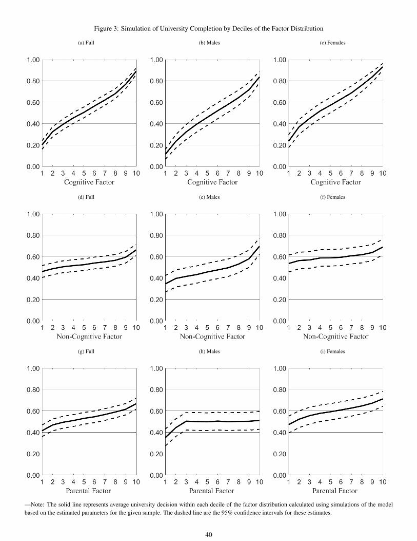
Figure 3: Simulation of University Completion by Deciles of the Factor Distribution

(a) Full (b) Males (c) Females

(d) Full (e) Males (f) Females

(g) Full (h) Males (i) Females

—Note: The solid line represents average university decision within each decile of the factor distribution calculated using simulations of the modelbased on the estimated parameters for the given sample. The dashed line are the 95% confidence intervals for these estimates.

40

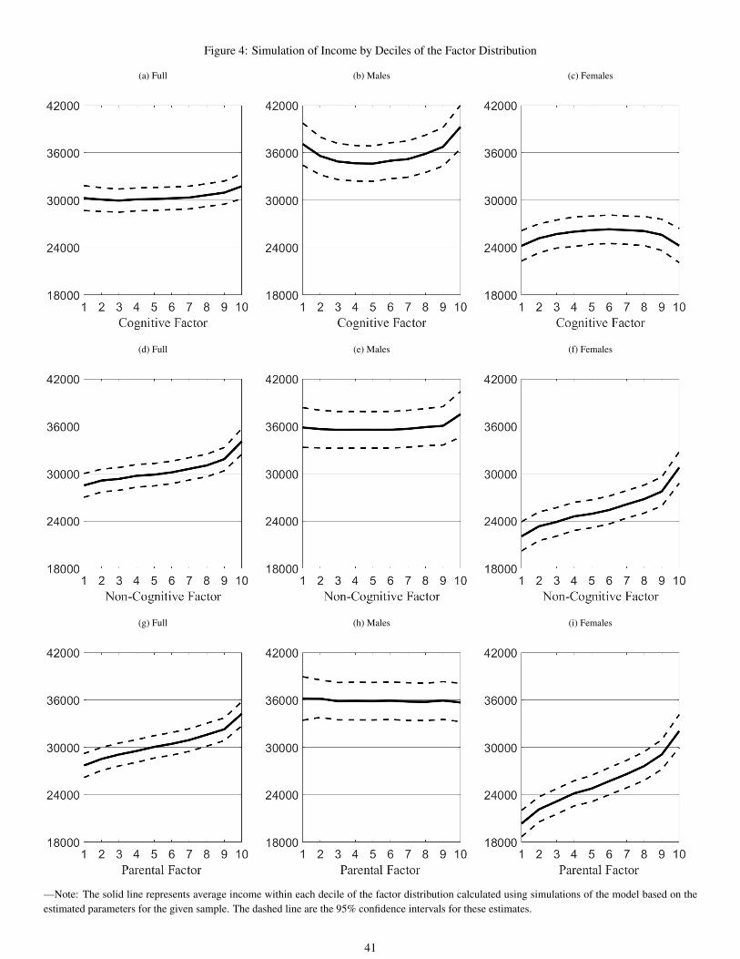
Figure 4: Simulation of Income by Deciles of the Factor Distribution

(a) Full (b) Males (c) Females

(d) Full (e) Males (f) Females

(g) Full (h) Males (i) Females

—Note: The solid line represents average income within each decile of the factor distribution calculated using simulations of the model based on theestimated parameters for the given sample. The dashed line are the 95% confidence intervals for these estimates.

41

Figure 5: Simulation of Income by University Completion Status by Deciles of the Factor Distribution

(a) Full (b) Males (c) Females

(d) Full (e) Males (f) Females

(g) Full (h) Males (i) Females

—Note: In this figure we present the average income within each decile of the factor by educational decision. The presented data are based on theestimated parameters for the given sample. The estimates and 95% confidence intervals for those that completed university in the simulations are givenby grey lines and shaded area. Similarity, the black lines give the same data for those who did not complete university.

42

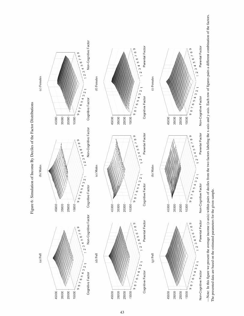
Figu

re6:

Sim

ulat

ion

ofIn

com

eB

yD

ecile

sof

the

Fact

orD

istr

ibut

ions

(a)F

ull

(b)M

ales

(c)F

emal

es

(d)F

ull

(e)M

ales

(f)F

emal

es

(g)F

ull

(h)M

ales

(i)F

emal

es

—N

ote:

Inth

isfig

ure

we

pres

entt

heav

erag

ein

com

e(z

-axi

s)w

ithin

pair

sof

deci

les

from

the

two

fact

ors

labe

ling

the

x-ax

isan

dy-

axis

.Eac

hro

wof

figur

espa

irs

adi

ffer

entc

ombi

natio

nof

the

fact

ors.

The

pres

ente

dda

taar

eba

sed

onth

ees

timat

edpa

ram

eter

sfo

rthe

give

nsa

mpl

e.

43

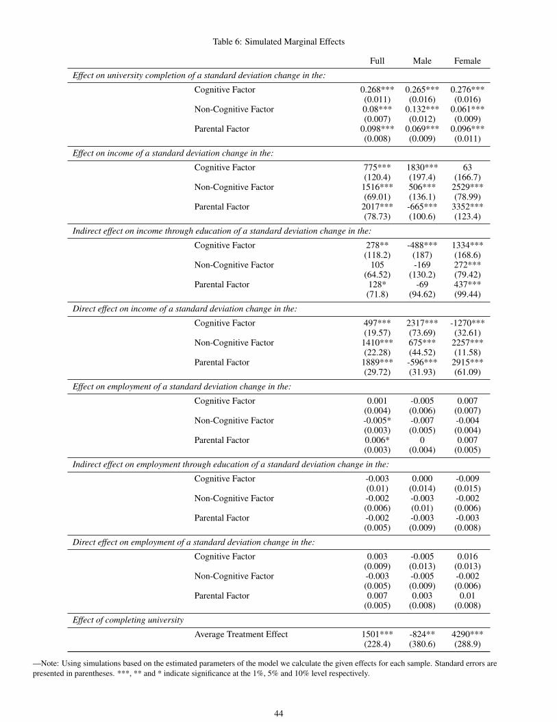
Table 6: Simulated Marginal Effects

Full Male Female

Effect on university completion of a standard deviation change in the:

Cognitive Factor 0.268*** 0.265*** 0.276***(0.011) (0.016) (0.016)

Non-Cognitive Factor 0.08*** 0.132*** 0.061***(0.007) (0.012) (0.009)

Parental Factor 0.098*** 0.069*** 0.096***(0.008) (0.009) (0.011)

Effect on income of a standard deviation change in the:

Cognitive Factor 775*** 1830*** 63(120.4) (197.4) (166.7)

Non-Cognitive Factor 1516*** 506*** 2529***(69.01) (136.1) (78.99)

Parental Factor 2017*** -665*** 3352***(78.73) (100.6) (123.4)

Indirect effect on income through education of a standard deviation change in the:

Cognitive Factor 278** -488*** 1334***(118.2) (187) (168.6)

Non-Cognitive Factor 105 -169 272***(64.52) (130.2) (79.42)

Parental Factor 128* -69 437***(71.8) (94.62) (99.44)

Direct effect on income of a standard deviation change in the:

Cognitive Factor 497*** 2317*** -1270***(19.57) (73.69) (32.61)

Non-Cognitive Factor 1410*** 675*** 2257***(22.28) (44.52) (11.58)

Parental Factor 1889*** -596*** 2915***(29.72) (31.93) (61.09)

Effect on employment of a standard deviation change in the:

Cognitive Factor 0.001 -0.005 0.007(0.004) (0.006) (0.007)

Non-Cognitive Factor -0.005* -0.007 -0.004(0.003) (0.005) (0.004)

Parental Factor 0.006* 0 0.007(0.003) (0.004) (0.005)

Indirect effect on employment through education of a standard deviation change in the:

Cognitive Factor -0.003 0.000 -0.009(0.01) (0.014) (0.015)

Non-Cognitive Factor -0.002 -0.003 -0.002(0.006) (0.01) (0.006)

Parental Factor -0.002 -0.003 -0.003(0.005) (0.009) (0.008)

Direct effect on employment of a standard deviation change in the:

Cognitive Factor 0.003 -0.005 0.016(0.009) (0.013) (0.013)

Non-Cognitive Factor -0.003 -0.005 -0.002(0.005) (0.009) (0.006)

Parental Factor 0.007 0.003 0.01(0.005) (0.008) (0.008)

Effect of completing university

Average Treatment Effect 1501*** -824** 4290***(228.4) (380.6) (288.9)

—Note: Using simulations based on the estimated parameters of the model we calculate the given effects for each sample. Standard errors arepresented in parentheses. ***, ** and * indicate significance at the 1%, 5% and 10% level respectively.

44

Online Appendix to How Skills and Parental Education Expectations

Influence Human Capital Acquisition and Early Labour Market Return to

Human Capital in Canada

Michael J. KottelenbergHuron University College

Steven F. LehrerQueen’s University, NYU-Shanghai and NBER

February 2019

Abstract

This is the online appendix for Kottelenberg and Lehrer (2019). We include five sections. We provide a description of thevariables, and their construction, in the first section. Second we provide the estimation results simulations not includedin Kottelenberg and Lehrer (2019) for the employment dependent variables. The third section presents estimates andsimulations of a two factor model in which the parenting factor is absent. In section 4, we reestimate the two factor modelwith a relax assumptions on the correlation between the factors and provide a description of the imputation procedureused in these estimates and the main text. In the final section we test the sensitivity of our model to the inclusion andexclusion of several key variables.

1

A Description of Variables

Cognitive Factor Variables

PISA Reading Score: PISA test measuring student’s reading literacy. The test assesses studentability to retrieve information from, understand and interpret, and reflectupon and evaluate written texts.

PISA Math Score: PISA test measuring student’s mathematical literacy. The test assesses stu-dent knowledge of rules and theorem and their ability to put mathematicalknowledge to problem solve within a variety of everyday contexts.

PISA Science Score: PISA test measuring student’s scientific literacy. The test assess under-standing of important scientific concepts alongside the ability to answerquestion via scientific evidence based inquiry and to apply these to theevaluation of other aspects of science and technology.

Non-Cognitive Factor Variables

Self-Efficacy Scale: Students belief about ability to understand the most difficult material pre-sented in readings, about their ability to do an excellent job on assignmentsand test, and about their ability to master the skills being taught.

Sense of Mastery Scale: Students feelings about being pushed around in life, about the dependencyof their future on themselves, about their ability to solve their own prob-lems, about their ability to change important things in their life, abouttheir helpless in dealing with the problems of life, about their control overthe things that happen to them, and about their ability to do just aboutanything they set their minds to.

Self Esteem Scale: Students feelings about being a person of worth, at least on an equal basiswith others, that they have a number of good qualities, that, all in all, theytend to feel that they are a failure, about their ability to do things as wellas most other people, that they do not have much to be proud of, that theyhave a positive attitude toward themselves, that, on the whole, they aresatisfied with themselves, about wishing they could like myself more, aboutbeing useless at times, and that at times they think they are no good atall.

Parental Factor Variables

Parent Educational Aspiration for Youth Parent’s answer to: “What is the highest level of education that you hopechild will get?” Coded with four possible values: 1, less than high school;2, high school diploma; 3 trade, vocational or college diploma; 4, universitydegree or beyond.

Importance of Post-Secondary Education(Parent’s Answer):

Parent’s answer to: “How important is it to you that child gets more edu-cation after high school?” Coded with four possible answers: not, slightly,fairly, and very important.

Importance of Post-Secondary Education(Youth’s Answer):

Youth’s answer to: “How important is it to your parent(s) that you getmore education after high school? ” Coded with four possible answers:not, slightly, fairly, and very important.

Other Covariates

Family Income: Income derived from wages/salaries, self employment, and governmentaltransfers and social assistance.

Wealth Index: Student reported availability of dishwasher, room of their own, educational,software, link to the internet, number of cell phones, television sets, com-puters, motor cars, and bathrooms in home.

continued on the next page...

2

Other Covariates

Non-Traditional Family: A family that is not made up of two biological parents.

Parental money for Post-Secondary Education: Has the parent ever taken a specific action towards ensuring that a childwill have money for education past high school.

Planning for Higher Education Among Friends: How many of the student’s closes friends are planning to further educationor training after high school. Coded with four possible answers none, some,most and all of them.

3

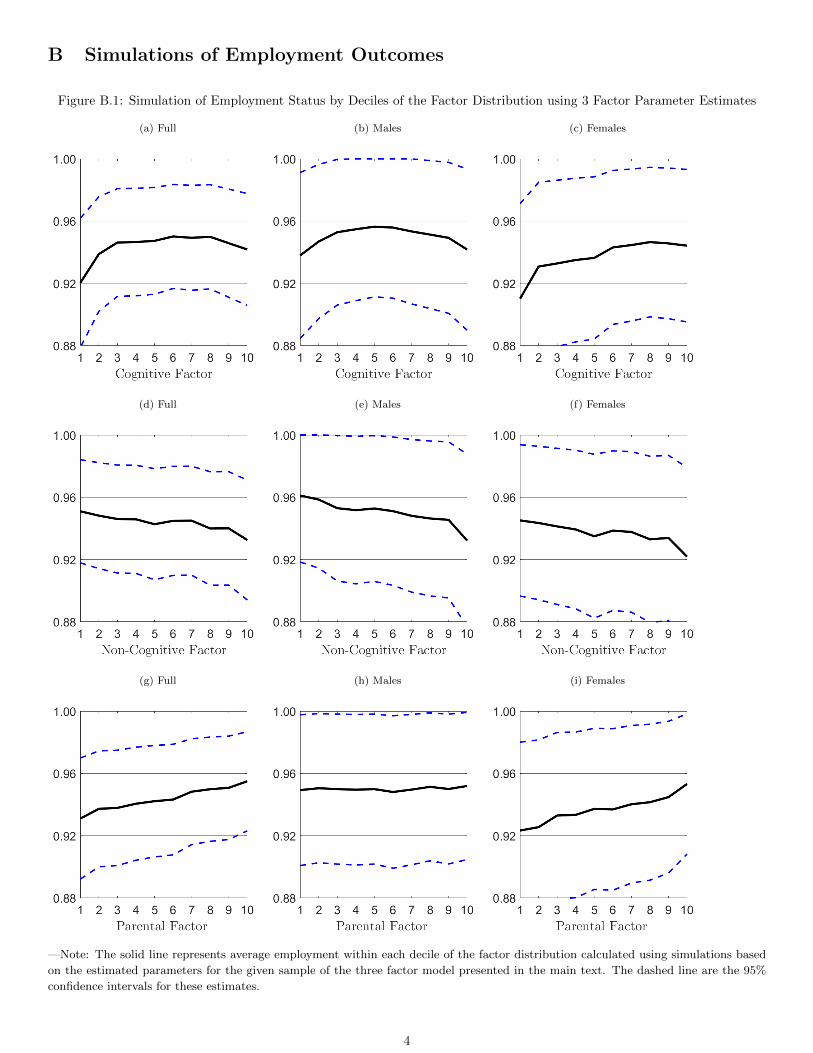
B Simulations of Employment Outcomes

Figure B.1: Simulation of Employment Status by Deciles of the Factor Distribution using 3 Factor Parameter Estimates

(a) Full (b) Males (c) Females

(d) Full (e) Males (f) Females

(g) Full (h) Males (i) Females

—Note: The solid line represents average employment within each decile of the factor distribution calculated using simulations based

on the estimated parameters for the given sample of the three factor model presented in the main text. The dashed line are the 95%

confidence intervals for these estimates.

4

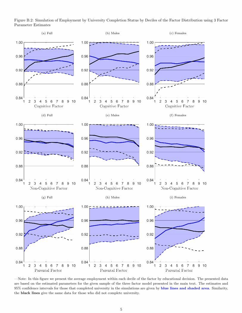
Figure B.2: Simulation of Employment by University Completion Status by Deciles of the Factor Distribution using 3 FactorParameter Estimates

(a) Full (b) Males (c) Females

(d) Full (e) Males (f) Females

(g) Full (h) Males (i) Females

—Note: In this figure we present the average employment within each decile of the factor by educational decision. The presented data

are based on the estimated parameters for the given sample of the three factor model presented in the main text. The estimates and

95% confidence intervals for those that completed university in the simulations are given by blue lines and shaded area. Similarity,

the black lines give the same data for those who did not complete university.

5

Fig

ure

B.3

:S

imu

lati

on

of

Em

plo

ym

ent

By

Dec

iles

of

the

Fac

tor

Dis

trib

uti

on

s

(a)FullSample

(b)Males

(c)Fem

ales

(d)FullSample

(e)Male

(f)Fem

ale

(g)FullSample

(h)Male

(i)Fem

ale

—N

ote

:In

this

figure

we

pre

sent

the

aver

age

emplo

ym

ent

(z-a

xis

)w

ithin

pair

sof

dec

iles

from

the

two

fact

ors

lab

elin

gth

ex-a

xis

and

y-a

xis

.E

ach

row

of

figure

spair

sa

diff

eren

t

com

bin

ati

on

of

the

fact

ors

.T

he

pre

sente

ddata

are

base

don

the

esti

mate

dpara

met

ers

for

the

giv

ensa

mple

.

6

C Basic Two Factor Model using Cognitive and Non-Cognitive Factors

In this section, we present the results of the estimation procedure using only the cognitive and non-cognitive factors. Weinclude estimates of the test score equations in Table C.1, the decision equations in Table C.2, and the outcomes in TableC.3. In this case we present several extra outcomes, whether a youth had used employment insurance or volunteered in thelast month, but only for the sample of youth who have completed 3 PISA tests and have complete cases.

The estimates in the test and decisions equations remain largely unchanged in terms of the influence of the factors inquestion. The coefficients for the impact of the factors on university completion from the two factor model are 0.855 and0.263 for the cognitive and non-cognitive factors respectively. These compare to estimates of 0.882 and 0.267 from the threefactor model. The majority of the estimated coefficients in these equation share similar sized differences. In terms the impactof the estimated factors on income, we note that in the absence of the parental factor that non-cognitive skills are much moreimportant for university graduates. The factor variables are otherwise of the same sign and significance as the estimates inthe three factor analysis. When examining the employment outcome we find this to also be true.

Figures C.1–C.4 present the simulations of the decision and outcomes as they vary with changes in the factor distributions.In Figure C.1 we note that in the absence of the parental factor their is less variance in the completion of university along thecognitive factor. At the first deciles the completion rate is around %35 and in the 10th deciles it is just under %80 comparedto %20 and %95 in the estimation with all three factors. The non-cognitive outcome impact on the education decision isnot largely unaffected in comparing the estimation strategies. In comparison to the analagous figures from the three factorestimation we see in figure C.2b a much larger impact of the non-cognitive factors on income at age 25 and in figure C.3bthat this effect is mostly driven by university graduates. This is not surprising as we noted above the parameter estimate ofthe impact of non-cognitive skills on income for graduates becomes not significant in this factor become insignificant in the3 factor model.

With regards to the additional outcomes presented in this appendix we find a relationship between the use of employmentinsurance the skills. Figures C.2e and C.2f suggests that there is little connection between the factors and employmentinsurance. Examination of the parameter estimates in table C.3 and highlighted in the simulations in figures C.3e and C.3fsuggest that the non-cognitive is statistically significant and that in case of both factors sign of the effect is different foreach educational statuses. Higher skill level alongside university completion suggests less use of employment insurance, theopposite is true for those who have not completed university. Finally, we see a positive but non-significant correlation betweenboth skills and volunteering at age 25. Figure C.4d highlights the joint impact of these skills.

7

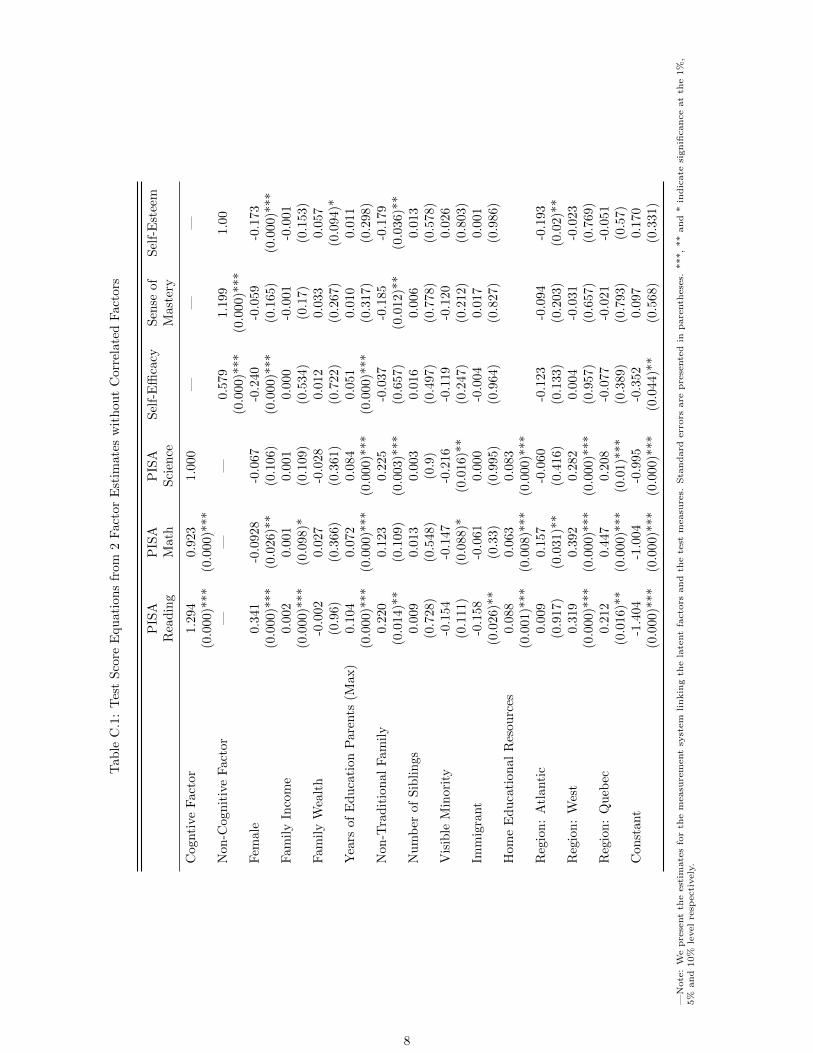
Tab

leC

.1:

Tes

tS

core

Equ

ati

on

sfr

om

2F

act

or

Est

imate

sw

ith

out

Corr

elate

dF

act

ors

PIS

AP

ISA

PIS

AS

elf-

Effi

cacy

Sen

seof

Sel

f-E

stee

mR

ead

ing

Math

Sci

ence

Mast

ery

Cog

nti

veF

acto

r1.2

94

0.9

23

1.0

00

——

—(0

.000)*

**

(0.0

00)*

**

Non

-Cog

nit

ive

Fac

tor

——

—0.5

79

1.1

99

1.0

0(0

.000)*

**

(0.0

00)*

**

Fem

ale

0.3

41

-0.0

928

-0.0

67

-0.2

40

-0.0

59

-0.1

73

(0.0

00)*

**

(0.0

26)*

*(0

.106)

(0.0

00)*

**

(0.1

65)

(0.0

00)*

**

Fam

ily

Inco

me

0.0

02

0.0

01

0.0

01

0.0

00

-0.0

01

-0.0

01

(0.0

00)*

**

(0.0

98)*

(0.1

09)

(0.5

34)

(0.1

7)

(0.1

53)

Fam

ily

Wea

lth

-0.0

02

0.0

27

-0.0

28

0.0

12

0.0

33

0.0

57

(0.9

6)

(0.3

66)

(0.3

61)

(0.7

22)

(0.2

67)

(0.0

94)*

Yea

rsof

Ed

uca

tion

Par

ents

(Max)

0.1

04

0.0

72

0.0

84

0.0

51

0.0

10

0.0

11

(0.0

00)*

**

(0.0

00)*

**

(0.0

00)*

**

(0.0

00)*

**

(0.3

17)

(0.2

98)

Non

-Tra

dit

ion

alF

amily

0.2

20

0.1

23

0.2

25

-0.0

37

-0.1

85

-0.1

79

(0.0

14)*

*(0

.109)

(0.0

03)*

**

(0.6

57)

(0.0

12)*

*(0

.036)*

*N

um

ber

ofS

ibli

ngs

0.0

09

0.0

13

0.0

03

0.0

16

0.0

06

0.0

13

(0.7

28)

(0.5

48)

(0.9

)(0

.497)

(0.7

78)

(0.5

78)

Vis

ible

Min

orit

y-0

.154

-0.1

47

-0.2

16

-0.1

19

-0.1

20

0.0

26

(0.1

11)

(0.0

88)*

(0.0

16)*

*(0

.247)

(0.2

12)

(0.8

03)

Imm

igra

nt

-0.1

58

-0.0

61

0.0

00

-0.0

04

0.0

17

0.0

01

(0.0

26)*

*(0

.33)

(0.9

95)

(0.9

64)

(0.8

27)

(0.9

86)

Hom

eE

du

cati

onal

Res

ourc

es0.0

88

0.0

63

0.0

83

(0.0

01)*

**

(0.0

08)*

**

(0.0

00)*

**

Reg

ion

:A

tlan

tic

0.0

09

0.1

57

-0.0

60

-0.1

23

-0.0

94

-0.1

93

(0.9

17)

(0.0

31)*

*(0

.416)

(0.1

33)

(0.2

03)

(0.0

2)*

*R

egio

n:

Wes

t0.3

19

0.3

92

0.2

82

0.0

04

-0.0

31

-0.0

23

(0.0

00)*

**

(0.0

00)*

**

(0.0

00)*

**

(0.9

57)

(0.6

57)

(0.7

69)

Reg

ion

:Q

ueb

ec0.2

12

0.4

47

0.2

08

-0.0

77

-0.0

21

-0.0

51

(0.0

16)*

*(0

.000)*

**

(0.0

1)*

**

(0.3

89)

(0.7

93)

(0.5

7)

Con

stan

t-1

.404

-1.0

04

-0.9

95

-0.3

52

0.0

97

0.1

70

(0.0

00)*

**

(0.0

00)*

**

(0.0

00)*

**

(0.0

44)*

*(0

.568)

(0.3

31)

—N

ote

:W

epre

sent

the

est

imate

sfo

rth

em

easu

rem

ent

syst

em

linkin

gth

ela

tent

facto

rsand

the

test

measu

res.

Sta

ndard

err

ors

are

pre

sente

din

pare

nth

ese

s.***,

**

and

*in

dic

ate

signifi

cance

at

the

1%

,5%

and

10%

level

resp

ecti

vely

.

8

Table C.2: Decision Equation from 2 Factor Estimates without Correlated Factors

University Completion

Cognitive Factor 0.855(0.000)***

Non-Cognitive Factor 0.283(0.000)***

Parental money for Post-Secondary Education (Y/N) 0.230(0.006)***

Importance of Post-Secondary Education 0.310(Youth’s answer about the parent’s) (0.000)***Female 0.537

(0.000)***Family Income 0.002

(0.133)Family Wealth 0.090

(0.12)Parental Education (Max) 0.172

(0.000)***Planning for Higher Education Among Friends 0.254

(0.000)***Immigrant Status -0.357

(0.001)***Non-Traditional Family 0.294

(0.038)**Region: Atlantic 0.375

(0.009)***Region: West 0.149

(0.264)Region: Quebec -0.189

(0.216)Constant -4.577

(0.000)***

—Note: We present the estimates and standard errors in parentheses of decision equation. ***, ** and * indicate significance at the 1%, 5% and 10% levelrespectively.

9

Figure C.1: Simulation of University Decision by Deciles of the Factor Distribution using 2 Factor Parameter Estimateswithout Correlated Factors

(a) University Decision (b) University Decision

—Note: The solid line represents the sample average of university completion within each decile of the factor distribution calculated

using simulations of the model based on the estimated parameters. The dashed line are the 95% confidence intervals for these

estimates.

10

Tab

leC

.3:

Ou

tcom

eE

qu

ati

on

from

2F

act

or

Mod

elw

ith

ou

tC

orr

elate

dF

act

ors

OutcomeEquation

Inco

me

Em

plo

yed

Volu

nte

er(O

nce

aM

onth

)E

mp

loym

ent

Insu

ran

ce

D=

1D

=0

D=

1D

=0

D=

1D

=0

D=

1D

=0

Cog

nit

ive

Fac

tor

392.

41-3

61.2

0-0

.015

0.0

43

0.0

67

-0.0

01

-0.0

33

0.0

20

(0.8

26)

(0.8

43)

(0.4

84)

(0.0

97)*

(0.0

73)*

(0.9

73)

(0.1

95)

(0.5

84)

Non

-Cog

nit

ive

Fac

tor

2812

.70

2167.0

9-0

.021

-0.0

05

0.0

31

0.0

10

-0.0

44

0.0

73

(0.0

55)*

(0.2

73)

(0.1

96)

(0.8

13)

(0.2

98)

(0.7

54)

(0.0

23)*

*(0

.049)*

*F

emal

e-3

660.

44-9

257.0

40.0

06

0.0

34

0.0

62

0.0

75

0.0

05

-0.0

65

(0.0

59)*

(0.0

00)*

**

(0.7

97)

(0.3

25)

(0.1

21)

(0.0

77)*

(0.8

41)

(0.1

76)

Exp

erie

nce

2489

.43

-244.6

7(0

.012

)**

(0.8

31)

Exp

erie

nce

Squ

ared

-373

.60

64.6

7(0

.000

)***

(0.5

09)

Reg

ion

:A

tlan

tic

-330

3.49

-7513.9

60.0

14

-0.0

70

0.0

41

0.0

74

0.0

53

0.1

66

(0.1

65)

(0.0

11)*

*(0

.649)

(0.1

04)

(0.4

08)

(0.1

57)

(0.1

16)

(0.0

05)*

**

Reg

ion

:Q

ueb

ec-1

852.

92-7

984.2

20.0

00

-0.0

84

-0.0

82

0.0

06

0.0

12

0.1

04

(0.5

05)

(0.0

08)*

**

(0.9

93)

(0.0

51)*

(0.1

48)

(0.9

06)

(0.7

52)

(0.0

8)*

Reg

ion

:W

est

913.

651329.5

9-0

.043

-0.0

80

-0.0

02

0.1

04

-0.0

09

0.0

58

(0.6

8)(0

.625)

(0.1

23)

(0.0

41)*

*(0

.96)

(0.0

28)*

*(0

.765)

(0.2

84)

Mar

ried

1843

6.22

9980.6

80.0

69

0.0

14

0.0

34

0.0

64

0.0

03

-0.0

50

(0.0

00)*

**(0

.003)*

**

(0.1

27)

(0.7

73)

(0.6

49)

(0.2

72)

(0.9

6)

(0.4

44)

Mar

ried

*F

emal

e-1

9645

.98

-13219.3

8-0

.156

-0.1

83

-0.0

55

-0.0

67

0.1

10

0.1

65

(0.0

00)*

**(0

.004)*

**

(0.0

05)*

**

(0.0

05)*

**

(0.5

44)

(0.3

99)

(0.0

77)*

(0.0

66)*

Com

mon

Law

8418

.59

12738.3

4-0

.048

0.0

80

-0.0

58

-0.0

26

-0.0

20

-0.0

40

(0.0

1)**

*(0

.000)*

**

(0.2

58)

(0.0

5)*

*(0

.4)

(0.5

93)

(0.6

66)

(0.4

83)

Com

mon

Law

*F

emal

e5.

78-1

2023.8

40.1

03

-0.1

13

-0.0

22

-0.0

48

0.0

48

0.1

29

(0.9

99)

(0.0

04)*

**

(0.0

47)*

*(0

.063)*

(0.7

95)

(0.5

18)

(0.4

08)

(0.1

24)

Imm

igra

nt

158.

81-1

341.1

5-0

.019

-0.0

43

0.0

03

-0.0

30

0.0

32

-0.0

47

(0.9

44)

(0.6

49)

(0.5

19)

(0.3

21)

(0.9

47)

(0.5

6)

(0.3

12)

(0.4

25)

Vis

ible

Min

orit

y-4

655.

09-5

839.4

7-0

.094

-0.0

26

-0.0

54

0.0

95

-0.0

46

-0.0

57

(0.1

33)

(0.1

93)

(0.0

15)*

*(0

.688)

(0.4

)(0

.222)

(0.2

84)

(0.5

19)

Nu

mb

erof

Ch

ild

ren

-149

56.8

1-5

233.3

00.0

83

-0.0

91

0.6

29

-0.0

88

-0.0

95

-0.1

33

(0.4

93)

(0.2

58)

(0.7

79)

(0.1

73)

(0.1

93)

(0.2

81)

(0.7

71)

(0.1

5)

Nu

mb

erof

Ch

ild

ren

*F

emal

e96

59.9

3-6

975.2

8-0

.356

-0.2

18

-1.0

93

0.0

37

-0.0

75

0.1

28

(0.6

83)

(0.2

44)

(0.2

65)

(0.0

11)*

*(0

.037)*

*(0

.722)

(0.8

31)

(0.2

83)

Urb

anC

omm

unit

y43

86.5

71147.9

30.0

16

0.0

06

0.0

61

0.0

74

0.0

75

0.1

30

(0.0

28)*

*(0

.537)

(0.5

27)

(0.8

23)

(0.1

43)

(0.0

23)*

*(0

.008)*

**

(0.0

00)*

**

Con

stan

t29

126.

8436210.1

90.9

40

1.0

17

0.3

48

0.0

89

0.0

73

0.1

91

(0.0

00)*

**(0

.000)*

**

(0.0

00)*

**

(0.0

00)*

**

(0.0

00)*

**

(0.1

75)

(0.0

66)*

(0.0

11)*

*

—N

ote

:W

epre

sent

the

est

imate

sand

standard

err

ors

inpare

nth

ese

sof

outc

om

eequati

on

for

four

outc

om

evari

able

s.***,

**

and

*in

dic

ate

signifi

cance

at

the

1%

,5%

and

10%

level

resp

ecti

vely

.

11

Fig

ure

C.2

:S

imu

lati

onof

Ou

tcom

esby

Dec

iles

of

the

Fact

or

Dis

trib

uti

on

usi

ng

2F

act

or

Para

met

erE

stim

ate

sw

ith

ou

tC

orr

elate

dF

act

ors

(a)Inco

me

(b)Inco

me

(c)Employmen

t(d

)Employmen

t

(e)Employmen

tInsu

rance

(f)Employmen

tInsu

rance

(g)Volunteer

(h)Volunteer

—N

ote

:F

or

each

outc

om

eth

eso

lid

line

repre

sents

the

sam

ple

aver

age

wit

hin

each

dec

ile

of

the

fact

or

dis

trib

uti

on

calc

ula

ted

usi

ng

sim

ula

tions

of

the

model

base

don

the

esti

mate

dpara

met

ers.

The

dash

edline

are

the

95%

confiden

cein

terv

als

for

thes

ees

tim

ate

s.

12

Fig

ure

C.3

:S

imu

lati

onof

Ou

tcom

esby

Dec

iles

of

the

Fact

or

Dis

trib

uti

on

usi

ng

2F

act

or

Para

met

erE

stim

ate

sw

ith

ou

tC

orr

elate

dF

act

ors

(a)Inco

me

(b)Inco

me

(c)Employmen

t(d

)Employmen

t

(e)Employmen

tInsu

rance

(f)Employmen

tInsu

rance

(g)Volunteer

(h)Volunteer

—N

ote

:In

this

figure

we

pre

sent

the

aver

age

outc

om

ew

ithin

each

dec

ile

of

the

fact

or

by

educa

tional

dec

isio

n.

The

pre

sente

ddata

are

base

don

the

esti

mate

dpara

met

ers

for

the

giv

ensa

mple

.T

he

esti

mate

sand

95%

confiden

cein

terv

als

for

those

that

com

ple

ted

univ

ersi

tyin

the

sim

ula

tions

are

giv

enbybluelinesand

shaded

are

a.

Sim

ilari

ty,

theblack

lines

giv

eth

esa

me

data

for

those

who

did

not

com

ple

teuniv

ersi

ty.

13

Figure C.4: Simulation of Outcomes By Deciles of the Factor Distributions using 2 Factor Parameter Estimates withoutCorrelated Factors

(a) Income (b) Employment

(c) Employment Insurance (d) Volunteers

—Note: In these figures we present the average outcome (z-axis) within pairs of deciles from the two factors labeling the x-axis and

y-axis. The presented data are based on the estimated parameters for the given sample.

14

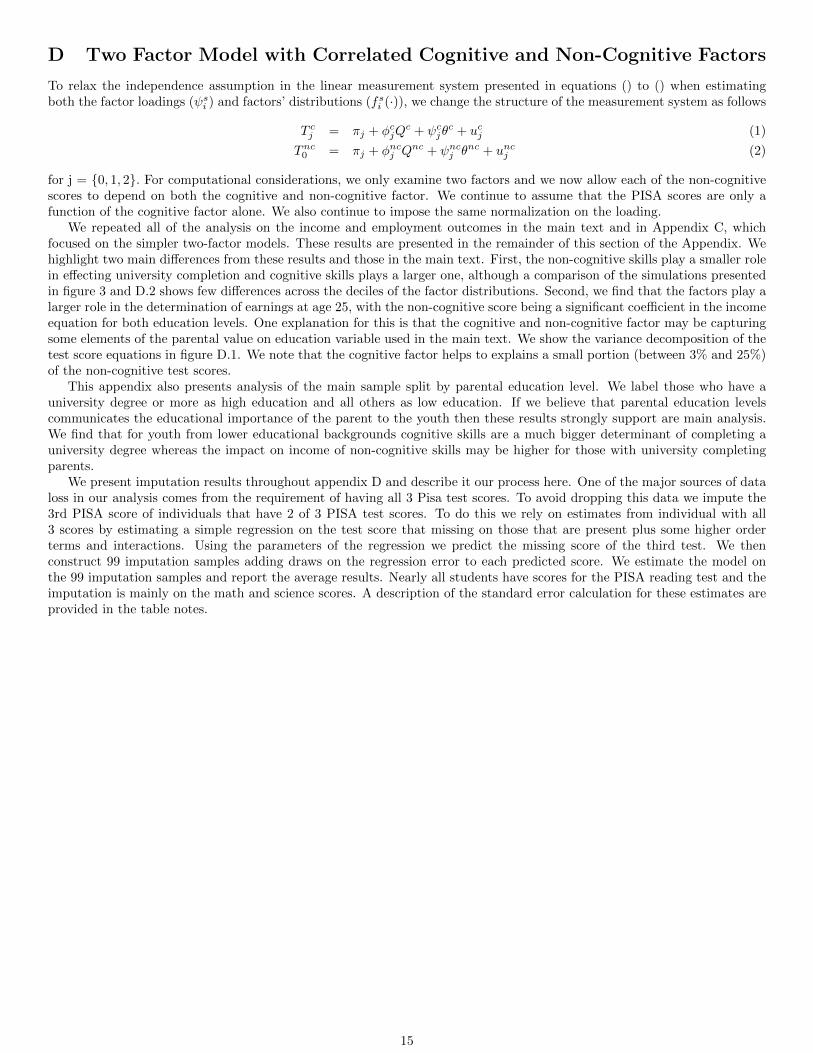
D Two Factor Model with Correlated Cognitive and Non-Cognitive Factors

To relax the independence assumption in the linear measurement system presented in equations () to () when estimatingboth the factor loadings (ψsi ) and factors’ distributions (fsi (·)), we change the structure of the measurement system as follows

T cj = πj + φcjQc + ψcjθ

c + ucj (1)

Tnc0 = πj + φncj Qnc + ψncj θ

nc + uncj (2)

for j = {0, 1, 2}. For computational considerations, we only examine two factors and we now allow each of the non-cognitivescores to depend on both the cognitive and non-cognitive factor. We continue to assume that the PISA scores are only afunction of the cognitive factor alone. We also continue to impose the same normalization on the loading.

We repeated all of the analysis on the income and employment outcomes in the main text and in Appendix C, whichfocused on the simpler two-factor models. These results are presented in the remainder of this section of the Appendix. Wehighlight two main differences from these results and those in the main text. First, the non-cognitive skills play a smaller rolein effecting university completion and cognitive skills plays a larger one, although a comparison of the simulations presentedin figure 3 and D.2 shows few differences across the deciles of the factor distributions. Second, we find that the factors play alarger role in the determination of earnings at age 25, with the non-cognitive score being a significant coefficient in the incomeequation for both education levels. One explanation for this is that the cognitive and non-cognitive factor may be capturingsome elements of the parental value on education variable used in the main text. We show the variance decomposition of thetest score equations in figure D.1. We note that the cognitive factor helps to explains a small portion (between 3% and 25%)of the non-cognitive test scores.

This appendix also presents analysis of the main sample split by parental education level. We label those who have auniversity degree or more as high education and all others as low education. If we believe that parental education levelscommunicates the educational importance of the parent to the youth then these results strongly support are main analysis.We find that for youth from lower educational backgrounds cognitive skills are a much bigger determinant of completing auniversity degree whereas the impact on income of non-cognitive skills may be higher for those with university completingparents.

We present imputation results throughout appendix D and describe it our process here. One of the major sources of dataloss in our analysis comes from the requirement of having all 3 Pisa test scores. To avoid dropping this data we impute the3rd PISA score of individuals that have 2 of 3 PISA test scores. To do this we rely on estimates from individual with all3 scores by estimating a simple regression on the test score that missing on those that are present plus some higher orderterms and interactions. Using the parameters of the regression we predict the missing score of the third test. We thenconstruct 99 imputation samples adding draws on the regression error to each predicted score. We estimate the model onthe 99 imputation samples and report the average results. Nearly all students have scores for the PISA reading test and theimputation is mainly on the math and science scores. A description of the standard error calculation for these estimates areprovided in the table notes.

15

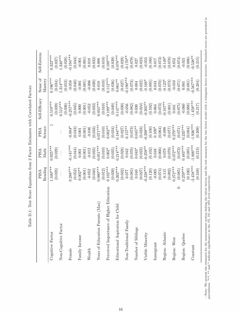
Tab

leD

.1:

Tes

tS

core

Equ

ati

on

sfr

om

2F

act

or

Est

imate

sw

ith

Corr

elate

dF

act

ors

PIS

AP

ISA

PIS

AS

elf-

Effi

cacy

Sen

seof

Sel

f-E

stee

mR

ead

ing

Math

Sci

ence

Mast

ery

Cog

nit

ive

Fac

tor

1.3

40***

0.9

25***

10.5

19***

0.1

96***

0.3

22***

(0.0

28)

(0.0

29)

(0.0

39)

(0.0

34)

(0.0

37)

Non

-Cog

nit

ive

Fac

tor

——

—0.5

12***

1.3

14***

1.3

40***

(0.0

36)

(0.0

53)

(0.0

28)

Fem

ale

0.2

88***

-0.1

41***

-0.0

84*

-0.2

57***

-0.0

58

-0.1

94***

(0.0

52)

(0.0

44)

(0.0

43)

(0.0

45)

(0.0

40)

(0.0

44)

Fam

ily

Inco

me

0.0

02**

0.0

01

0.0

01

0.0

00

-0.0

01

-0.0

01

(0.0

01)

(0.0

01)

(0.0

01)

(0.0

01)

(0.0

01)

(0.0

01)

Wea

lth

-0.0

52

-0.0

12

-0.0

46

-0.0

52

-0.0

06

0.0

18

(0.0

40)

(0.0

33)

(0.0

33)

(0.0

33)

(0.0

30)

(0.0

32)

Yea

rsof

Ed

uca

tion

Par

ents

(Max

)0.0

80***

0.0

51***

0.0

71***

0.0

34***

0.0

10

0.0

08

(0.0

12)

(0.0

10)

(0.0

10)

(0.0

10)

(0.0

10)

(0.0

10)

Per

ceiv

edIm

por

tan

ceof

Hig

her

Ed

uca

tion

0.1

02***

0.0

62*

0.0

82**

0.1

89***

0.1

12***

0.1

00***

(0.0

39)

(0.0

35)

(0.0

34)

(0.0

40)

(0.0

36)

(0.0

39)

Ed

uca

tion

alA

spir

atio

nfo

rC

hil

d0.2

62***

0.2

14***

0.1

84***

0.1

47***

0.0

61**

0.0

78***

(0.0

32)

(0.0

28)

(0.0

27)

(0.0

30)

(0.0

27)

(0.0

29)

Non

-Tra

dit

ion

alF

amil

y0.0

77

0.0

42

0.1

57**

-0.0

56

-0.1

90***

-0.1

70**

(0.0

85)

(0.0

76)

(0.0

73)

(0.0

82)

(0.0

73)

(0.0

79)

Nu

mb

erof

Sib

lin

gs0.0

40

0.0

43*

0.0

45**

0.0

30

0.0

04

0.0

27

(0.0

27)

(0.0

23)

(0.0

23)

(0.0

24)

(0.0

22)

(0.0

23)

Vis

ible

Min

orit

y-0

.328***

-0.2

59**

-0.2

99***

-0.2

05**

-0.1

68*

-0.0

53

(0.1

20)

(0.1

02)

(0.1

00)

(0.1

02)

(0.0

95)

(0.1

00)

Imm

igra

nt

-0.0

05

0.0

48

0.1

09*

0.0

64

0.0

43

0.0

17

(0.0

74)

(0.0

66)

(0.0

64)

(0.0

73)

(0.0

70)

(0.0

73)

Reg

ion

:A

tlan

tic

-0.1

15

0.0

79

-0.0

98

-0.1

67**

-0.1

23*

-0.1

49*

(0.0

92)

(0.0

79)

(0.0

77)

(0.0

81)

(0.0

73)

(0.0

78)

Reg

ion

:W

est

0.2

72***

0.3

72***

0.2

79***

0.0

41

-0.0

10

0.0

52

0(0

.085)

(0.0

73)

(0.0

71)

(0.0

75)

(0.0

71)

(0.0

74)

Reg

ion

:Q

ueb

ec0.2

59***

0.4

83***

0.2

35***

-0.0

60

0.0

01

-0.0

21

(0.1

00)

(0.0

85)

(0.0

84)

(0.0

88)

(0.0

81)

(0.0

86)

Con

stan

t-2

.458***

-1.8

00***

-1.9

36***

-1.4

59***

-0.5

67***

-0.5

38**

(0.2

49)

(0.2

13)

(0.2

09)

(0.2

17)

(0.2

04)

(0.2

15)

—N

ote

:W

epre

sent

the

est

imate

sfo

rth

em

easu

rem

ent

syst

em

linkin

gth

ela

tent

facto

rsand

the

test

measu

res

for

the

two

facto

rm

odel

wit

ha

tria

ngula

rfa

cto

rst

ructu

re.

Sta

ndard

err

ors

are

pre

sente

din

pare

nth

ese

s.***,

**

and

*in

dic

ate

signifi

cance

at

the

1%

,5%

and

10%

level

resp

ecti

vely

.

16

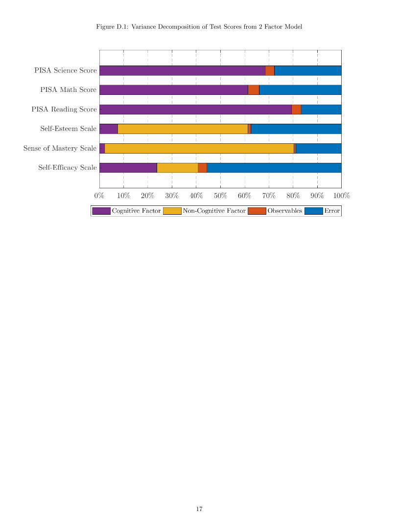
Figure D.1: Variance Decomposition of Test Scores from 2 Factor Model

17

Tab

leD

.2:

Dec

isio

nE

qu

ati

on

from

2F

act

or

Est

imate

sw

ith

Corr

elate

dF

act

ors

Fu

llIm

pu

tati

on

Male

Fem

ale

Low

Hig

hE

du

cati

on

Ed

uca

tion

Cog

nit

ive

Fac

tor

0.9

57***

0.9

18

0.9

16***

1.1

19***

1.1

02***

0.8

68***

(0.0

86)

(0.0

32)

(0.1

18)

(0.1

53)

(0.1

15)

(0.1

62)

Non

-Cog

nit

ive

Fac

tor

0.1

33**

0.1

78

0.2

02*

0.0

97

0.1

01

0.2

50*

(0.0

61)

(0.0

08)

(0.1

05)

(0.0

80)

(0.0

73)

(0.1

34)

Imp

orta

nce

ofP

ost-

Sec

ond

ary

Ed

uca

tion

0.2

80***

0.2

41

0.3

69*

**

0.2

13**

0.3

52***

0.1

03

(Ch

ild

’sA

nsw

erab

out

Par

ents

)(0

.073)

(0.0

03)

(0.1

06)

(0.1

05)

(0.0

84)

(0.1

75)

Ed

uca

tion

alA

spir

atio

nfo

rC

hil

d0.4

61***

0.5

30.4

72***

0.4

59***

0.4

26***

0.5

78***

(0.0

54)

(0.0

03)

(0.0

79)

(0.0

75)

(0.0

63)

(0.1

26)

Par

enta

lm

oney

for

Pos

t-S

econ

dar

yE

du

cati

on

0.1

97**

0.1

86

0.2

86**

0.1

29

0.1

24

0.6

33***

(0.0

85)

(0.0

06)

(0.1

25)

(0.1

20)

(0.1

00)

(0.1

90)

Fem

ale

0.5

32***

0.4

33

0.5

66***

0.6

47***

(0.0

78)

(0.0

03)

(0.0

94)

(0.1

64)

Fam

ily

Inco

me

0.0

01

0.0

01

0.0

00

0.0

02

0.0

02

0.0

00

(0.0

01)

(0)

(0.0

01)

(0.0

02)

(0.0

02)

(0.0

02)

Fam

ily

Wea

lth

0.0

41

0.0

64

-0.0

17

0.1

12

0.0

83

0.0

99

(0.0

56)

(0.0

02)

(0.0

79)

(0.0

84)

(0.0

68)

(0.1

11)

Par

enta

lE

du

cati

on(M

ax)

0.1

58***

0.1

56

0.1

26*

**

0.1

69***

——

(0.0

19)

(0.0

01)

(0.0

26)

(0.0

27)

Pla

nn

ing

for

Hig

her

Ed

uca

tion

(Am

on

gF

rien

ds)

0.2

32***

0.2

29

0.3

76*

**

0.1

06

0.2

79***

0.1

40

(0.0

57)

(0.0

03)

(0.0

83)

(0.0

82)

(0.0

69)

(0.1

18)

Imm

igra

nt

Sta

tus

-0.1

82*

-0.2

63

-0.4

92***

0.1

54

-0.2

80**

-0.1

69

(0.1

09)

(0.0

03)

(0.1

57)

(0.1

55)

(0.1

42)

(0.1

93)

Non

-Tra

dit

ion

alF

amil

y0.2

06

-0.0

34

-0.0

37

0.4

56**

0.1

78

-0.2

46

(0.1

37)

(0.0

04)

(0.1

92)

(0.2

09)

(0.1

61)

(0.3

02)

Reg

ion

:A

tlan

tic

0.2

54*

0.4

04

0.0

73

0.3

93**

0.4

52***

0.0

32

(0.1

39)

(0.0

04)

(0.2

03)

(0.1

97)

(0.1

71)

(0.2

81)

Reg

ion

:W

est

0.1

19

0.2

75

0.1

63-0

.005

0.4

01**

-0.1

98

(0.1

30)

(0.0

04)

(0.1

91)

(0.1

81)

(0.1

61)

(0.2

50)

Reg

ion

:Q

ueb

ec-0

.250*

-0.0

53

-0.3

89*

-0.2

48

-0.1

31

-0.0

95

(0.1

49)

(0.0

03)

(0.2

15)

(0.2

12)

(0.1

86)

(0.2

94)

Con

stan

t-5

.940***

-6.0

57

-5.9

51*

**

-5.2

11***

-4.4

00***

-3.0

36***

(0.4

60)

(0.0

3)

(0.6

65)

(0.6

51)

(0.4

86)

(0.8

50)

—N

ote

:W

epre

sent

the

est

imate

sand

standard

err

ors

inpare

nth

ese

sof

decis

ion

equati

on

for

four

sam

ple

s.For

the

imputa

tion

sam

ple

,w

epre

sent

the

avera

ge

est

imate

acro

ssth

eim

puta

tions

itera

tions,βI.

The

standard

err

or

inth

eim

puta

tion

model,sβI

isgiv

en

by√ w

+(1

+1 m

)Bw

herem

isth

enum

ber

of

imputa

tions,w

=1 m

∑ m i=1si β

andB

=1

m−

1

∑ m i=1(βi m

−βI)2

.***,

**

and

*in

dic

ate

signifi

cance

at

the

1%

,5%

and

10%

level

resp

ecti

vely

.

18

Tab

leD

.3:

Ou

tcom

eE

qu

ati

on

from

2F

act

or

Mod

elw

ith

Corr

elate

dF

act

ors

:In

com

e

Fu

llIm

pu

tati

on

Male

Fem

ale

Low

Ed

uca

tion

Hig

hE

du

cati

on

D=

0D

=1

D=

0D

=1

D=

0D

=1

D=

0D

=1

D=

0D

=1

D=

0D

=1

Cog

nit

ive

Fac

tor

1651

1800

1058

1651

2420

-1790

2473

4886*

3030

245

-3887

1933

(168

6)(1

527)

(118

9)

(1071)

(1960)

(2134)

(240

4)

(2593)

(1971)

(2039)

(3261)

(2419)

Non

-Cog

nit

ive

2256

*22

37*

1381

*66

2032

2427**

2246

521

1740

2203

4440

3029*

Fac

tor

(134

8)(1

148)

(715

.5)

(583.4

)(1

347)

(1187)

(235

9)

(2330)

(1479)

(1491)

(3229)

(1799)

Fem

ale

-915

0***

-390

7**

-976

5***

-3248***

——

——

-7642***

-6026**

-13726***

-592

(243

3)(1

928)

(128

4)

(961.9

)(2

723)

(2538)

(5063)

(2935)

Exp

erie

nce

-260

2519

**-2

34798*

-402

3847***

12874

-182

2821**

-2708

2326

(114

2)(9

94)

(508

.1)

(442)

(1337)

(1265)

(1657)

(1694)

(1307)

(1307)

(2279)

(1516)

Exp

erie

nce

69-3

72**

*4

-171***

27

-553***

86

-196

64

-425***

274

-339**

Squ

ared

(98)

(106

)(3

9.34

)(4

3.9

2)

(116)

(149)

(140)

(164)

(114)

(138)

(183)

(164)

Mar

ried

9969

***

1836

3***

8279

***

12988***

-2172

-1033

9238

**

17386***

10709***

17840***

8395

18205***

(326

8)(3

493)

(172

8)

(1894)

(2356)

(2307)

(374

6)

(3882)

(3599)

(4510)

(7185)

(5470)

Mar

ried

*F

emal

e-1

3547

***

-194

41**

*-1

2018

***

-10724***

——

——

-13914***

-20146***

-22725**

-16980**

(451

0)(4

287)

(237

7)

(2289)

(4923)

(5431)

(10938)

(6985)

Com

mon

Law

1326

2***

7783

**82

58**

*8183***

-362

9309***

13369***

6523*

13602***

2154

14067**

14884***

(279

8)(3

294)

(147

9)

(1719)

(2379)

(2199)

(321

3)

(3698)

(3161)

(4406)

(5635)

(4896)

Com

mon

Law

-127

05**

*79

4-6

146*

**

-1568

—-

—-

—-

—-

-14202***

6318

-7926

-5796

*F

emal

e(4

199)

(404

0)(2

149)

(2121)

(4657)

(5393)

(9433)

(6050)

Imm

igra

nt

-135

28

1009

1435

-3426

-5668**

733

7219**

-1380

-3336

-4150

2283

(292

9)(2

231)

(156

3)

(1171)

(3175)

(2773)

(455

2)

(3656)

(3377)

(3277)

(5341)

(3024)

Vis

ible

Min

orit

y-6

151

-507

8-6

165*

*-1

111

-11270**

-4055

-502

-6778

-1028

-8726*

-16148**

-3128

(447

5)(3

102)

(254

9)

(1645)

(5216)

(3965)

(665

3)

(4881)

(5424)

(4479)

(7312)

(4184)

Nu

mb

erof

-519

5-1

6237

-478

1*15782*

-10229***

-2945

-5696

-16145

-1127

23354

-22553**

-16102

Ch

ild

ren

(461

1)(2

1824

)(2

705)

(8141)

(2784)

(8157)

(527

1)

(24116)

(5172)

(15036)

(9509)

(20847)

Nu

mb

erof

-639

111

298

-377

0-2

6084***

—-

—-

—-

—-

-12051*

-22927

42102**

-16898

Ch

ild

ren

*F

emal

e(5

968)

(236

02)

(324

1)

(8903)

(6484)

(14987)

(21123)

(29630)

Urb

anC

omm

un

ity

1160

4300

**13

16573

-3054

3232

4752

*6695*

754

4911**

2622

1944

(185

4)(1

989)

(978

.9)

(1015)

(2016)

(2185)

(285

3)

(3969)

(2023)

(2402)

(4728)

(3681)

Reg

ion

:A

tlan

tic

-746

5**

-315

2-6

584*

**

-2256*

-6510**

-3673

-7700*

-2677

-7410**

-686

-9057

-6962**

(295

2)(2

378)

(150

3)

(1226)

(3243)

(2703)

(448

1)

(4362)

(3286)

(3237)

(6209)

(3536)

Reg

ion

:Q

ueb

ec-8

301*

**-1

619

-471

8***

-1873

-6095*

-2824

-8523*

861

-7608**

1346

-11028*

-4872

(299

0)(2

781)

(154

5)

(1399)

(3430)

(3268)

(449

1)

(4900)

(3328)

(3874)

(6297)

(3931)

Reg

ion

:W

est

1424

1147

3480

**

4907***

-2705

430

490

63618

2510

2757

-2140

-78

(269

9)(2

217)

(140

3)

(1129)

(2970)

(2613)

(413

9)

(3865)

(3040)

(3070)

(5395)

(3183)

Con

stan

t36

482*

**29

132*

**36

144*

**

30493***

34232***

29400***

30174***

24000***

35554***

32792***

46315***

26061***

(481

5)(3

230)

(241

4)

(1666)

(5294)

(3615)

(723

5)

(5411)

(5485)

(4644)

(9137)

(4532)

—N

ote

:W

epre

sent

the

est

imate

sand

standard

err

ors

inpare

nth

ese

sfo

routc

om

eequati

ons

exam

inin

gem

plo

ym

ent.

For

the

imputa

tion

sam

ple

,w

epre

sent

the

avera

ge

est

imate

acro

ssth

eim

puta

tions

itera

tions,βI.

The

standard

err

or

inth

eim

puta

tion

model,sβI

isgiv

en

by√ w

+(1

+1 m

)Bw

herem

isth

enum

ber

of

imputa

tions,w

=1 m

∑ m i=1si β

andB

=1

m−

1

∑ m i=1(βi m

−βI)2

.***,

**

and

*in

dic

ate

signifi

cance

at

the

1%

,5%

and

10%

level

resp

ecti

vely

.

19

Tab

leD

.4:

Ou

tcom

eE

qu

ati

on

from

2F

act

or

Mod

elw

ith

Corr

elate

dF

act

ors

:E

mp

loym

ent

Fu

llIm

pu

tati

on

Male

Fem

ale

Low

Ed

uca

tion

Hig

hE

du

cati

on

D=

0D

=1

D=

0D

=1

D=

0D

=1

D=

0D

=1

D=

0D

=1

D=

0D

=1

Cog

nit

ive

Fac

tor

0.02

7-0

.021

0.01

1-0

.025**

0.0

33

-0.0

34

0.0

33

-0.0

06

0.0

49*

-0.0

32

0.0

34

-0.0

17

(0.0

24)

(0.0

19)

(0.0

17)

(0.0

12)

(0.0

45)

(0.0

27)

(0.0

27)

(0.0

31)

(0.0

29)

(0.0

24)

(0.0

44)

(0.0

31)

Non

-Cog

nit

ive

-0.0

02-0

.024

*-0

.007

0.0

01

-0.0

14

-0.0

22

0.0

18

-0.0

39

-0.0

06

-0.0

12

0.0

40

0.0

19

Fac

tor

(0.0

19)

(0.0

15)

(0.0

1)(0

.007)

(0.0

31)

(0.0

17)

(0.0

27)

(0.0

27)

(0.0

21)

(0.0

18)

(0.0

45)

(0.0

22)

Fem

ale

0.03

20.

005

0.00

80.0

17

——

——

0.0

55

-0.0

04

0.0

25

0.0

38

(0.0

35)

(0.0

24)

(0.0

18)

(0.0

11)

(0.0

39)

(0.0

30)

(0.0

71)

(0.0

36)

Mar

ried

0.01

40.

067

0.01

20.0

27

-0.1

58***

-0.0

97***

0.0

08

0.0

62

0.0

41

0.0

05

-0.0

65

0.1

02

(0.0

47)

(0.0

45)

(0.0

24)

(0.0

22)

(0.0

52)

(0.0

32)

(0.0

43)

(0.0

47)

(0.0

51)

(0.0

53)

(0.1

01)

(0.0

66)

Mar

ried

*F

emal

e-0

.183

***

-0.1

54**

*-0

.13*

**-0

.077***

-0.1

95***

-0.1

08*

-0.5

68***

-0.2

41***

(0.0

65)

(0.0

56)

(0.0

34)

(0.0

27)

(0.0

70)

(0.0

63)

(0.1

54)

(0.0

85)

Com

mon

Law

0.08

0**

-0.0

500.

024

0.0

24

-0.0

41

0.0

58*

0.0

80**

-0.0

67

0.0

96**

-0.0

99*

0.0

37

0.0

58

(0.0

41)

(0.0

42)

(0.0

21)

(0.0

2)

(0.0

53)

(0.0

30)

(0.0

37)

(0.0

44)

(0.0

45)

(0.0

51)

(0.0

79)

(0.0

60)

Com

mon

Law

-0.1

12*

0.10

7**

-0.0

38-0

.006

-0.1

55**

0.1

40**

0.0

07

-0.0

33

*F

emal

e(0

.061

)(0

.052

)(0

.03)

(0.0

25)

(0.0

66)

(0.0

63)

(0.1

32)

(0.0

74)

Imm

igra

nt

-0.0

36-0

.021

0.02

00.0

06

-0.0

52

-0.0

72*

-0.0

13

0.0

43

-0.0

21

-0.0

05

-0.1

55**

-0.0

06

(0.0

43)

(0.0

29)

(0.0

22)

(0.0

13)

(0.0

71)

(0.0

37)

(0.0

52)

(0.0

45)

(0.0

48)

(0.0

38)

(0.0

75)

(0.0

37)

Vis

ible

Min

orit

y-0

.024

-0.0

97**

0.00

4-0

.029

-0.0

58

-0.1

49***

0.0

21

-0.0

40

0.0

20

-0.0

82

-0.1

62

-0.0

44

(0.0

64)

(0.0

39)

(0.0

36)

(0.0

19)

(0.1

11)

(0.0

53)

(0.0

76)

(0.0

57)

(0.0

77)

(0.0

52)

(0.1

03)

(0.0

51)

Nu

mb

erof

-0.0

870.

094

-0.0

200.0

76

-0.3

03***

-0.2

77**

-0.0

89

0.0

80

-0.0

11

-0.1

47

-0.4

09***

0.0

92

Ch

ild

ren

(0.0

67)

(0.2

95)

(0.0

38)

(0.1

)(0

.062)

(0.1

18)

(0.0

61)

(0.3

05)

(0.0

73)

(1494.4

34)

(0.1

33)

(0.2

53)

Nu

mb

erof

-0.2

21**

*-0

.369

-0.0

83*

-0.2

15**

-0.2

95***

-0.0

32

0.4

31

-0.9

38***

Ch

ild

ren

*F

emal

e(0

.086

)(0

.319

)(0

.046

)(0

.108)

(0.0

92)

(1494.4

34)

(0.2

97)

(0.3

60)

Urb

anC

omm

un

ity

0.00

40.

015

-0.0

24*

0.0

13

-0.0

26

0.0

35

0.0

32

-0.0

27

0.0

10

0.0

33

-0.0

06

-0.0

75*

(0.0

27)

(0.0

26)

(0.0

14)

(0.0

12)

(0.0

45)

(0.0

30)

(0.0

33)

(0.0

47)

(0.0

29)

(0.0

28)

(0.0

66)

(0.0

45)

Reg

ion

:A

tlan

tic

-0.0

72*

0.01

6-0

.029

0.0

13

-0.0

98

0.0

09

-0.0

48

0.0

22

-0.0

49

0.0

10

-0.1

28

-0.0

20

(0.0

43)

(0.0

30)

(0.0

21)

(0.0

14)

(0.0

73)

(0.0

37)

(0.0

51)

(0.0

52)

(0.0

47)

(0.0

38)

(0.0

87)

(0.0

43)

Reg

ion

:Q

ueb

ec-0

.083

*0.

002

-0.0

18-0

.026

-0.0

90

-0.0

20

-0.0

70

0.0

44

-0.0

67

0.0

38

-0.1

28

0.0

08

(0.0

43)

(0.0

34)

(0.0

22)

(0.0

16)

(0.0

76)

(0.0

43)

(0.0

52)

(0.0

57)

(0.0

47)

(0.0

45)

(0.0

89)

(0.0

48)

Reg

ion

:W

est

-0.0

80**

-0.0

42-0

.04*

*0.0

05

-0.1

41**

-0.0

34

-0.0

33

-0.0

41

-0.0

53

-0.0

28

-0.1

59**

-0.0

42

(0.0

39)

(0.0

28)

(0.0

2)(0

.013)

(0.0

67)

(0.0

36)

(0.0

47)

(0.0

46)

(0.0

43)

(0.0

36)

(0.0

76)

(0.0

39)

Con

stan

t1.

009*

**0.

940*

**0.

917*

**0.9

02***

1.1

02***

0.9

93***

0.9

54***

0.8

82***

1.0

39***

1.0

02***

1.2

96***

0.9

77***

(0.0

54)

(0.0

35)

(0.0

27)

(0.0

16)

(0.0

87)

(0.0

42)

(0.0

66)

(0.0

52)

(0.0

78)

(0.0

54)

(0.1

29)

(0.0

55)

—N

ote

:W

epre

sent

the

est

imate

sand

standard

err

ors

inpare

nth

ese

sfo

routc

om

eequati

ons

exam

inin

gem

plo

ym

ent.

For

the

imputa

tion

sam

ple

,w

epre

sent

the

avera

ge

est

imate

acro

ssth

eim

puta

tions

itera

tions,βI.

The

standard

err

or

inth

eim

puta

tion

model,sβI

isgiv

en

by√ w

+(1

+1 m

)Bw

herem

isth

enum

ber

of

imputa

tions,w

=1 m

∑ m i=1si β

andB

=1

m−

1

∑ m i=1(βi m

−βI)2

.***,

**

and

*in

dic

ate

signifi

cance

at

the

1%

,5%

and

10%

level

resp

ecti

vely

.

20

Fig

ure

D.2

:S

imu

lati

onof

Un

iver

sity

Com

ple

tion

by

Dec

iles

of

the

Fact

or

Dis

trib

uti

on

usi

ng

2F

act

or

Para

met

erE

stim

ate

s

(a)Full

(b)Males

(c)Fem

ales

(d)Low

Educa

tion

(e)HighEduca

tion

(f)Full

(g)Males

(h)Fem

ales

(i)Low

Educa

tion

(j)HighEduca

tion

—N

ote

:T

he

solid

line

repre

sents

aver

age

univ

ersi

tydec

isio

nw

ithin

each

dec

ile

of

the

fact

or

dis

trib

uti

on

calc

ula

ted

usi

ng

sim

ula

tions

of

the

model

base

don

the

esti

mate

dpara

met

ers

for

the

giv

ensa

mple

.T

he

dash

edline

are

the

95%

confiden

cein

terv

als

for

thes

ees

tim

ate

s.

21

Fig

ure

D.3

:S

imu

lati

onof

Inco

me

by

Dec

iles

of

the

Fact

or

Dis

trib

uti

on

usi

ng

2F

act

or

Para

met

erE

stim

ate

s

(a)Full

(b)Males

(c)Fem

ales

(d)Low

Educa

tion

(e)HighEduca

tion

(f)Full

(g)Males

(h)Fem

ales

(i)Low

Educa

tion

(j)HighEduca

tion

—N

ote

:T

he

solid

line

repre

sents

aver

age

inco

me

wit

hin

each

dec

ile

of

the

fact

or

dis

trib

uti

on

calc

ula

ted

usi

ng

sim

ula

tions

of

the

model

base

don

the

esti

mate

dpara

met

ers

for

the

giv

ensa

mple

.T

he

dash

edline

are

the

95%

confiden

cein

terv

als

for

thes

ees

tim

ate

s.

22

Fig

ure

D.4

:S

imu

lati

onof

Inco

me

by

Un

iver

sity

Com

ple

tion

Sta

tus

by

Dec

iles

of

the

Fact

or

Dis

trib

uti

on

usi

ng

2F

act

or

Para

met

erE

stim

ate

s

(a)Full

(b)Males

(c)Fem

ales

(d)Low

Educa

tion

(e)HighEduca

tion

(f)Full

(g)Males

(h)Fem

ales

(i)Low

Educa

tion

(j)HighEduca

tion

—N

ote

:In

this

figure

we

pre

sent

the

aver

age

inco

me

wit

hin

each

dec

ile

of

the

fact

or

by

educa

tional

dec

isio

n.

The

pre

sente

ddata

are

base

don

the

esti

mate

dpara

met

ers

for

the

giv

ensa

mple

.T

he

esti

mate

sand

95%

confiden

cein

terv

als

for

those

that

com

ple

ted

univ

ersi

tyin

the

sim

ula

tions

are

giv

enbybluelinesand

shaded

are

a.

Sim

ilari

ty,

theblack

lines

giv

eth

esa

me

data

for

those

who

did

not

com

ple

teuniv

ersi

ty.

23

Figure D.5: Simulation of Income By Deciles of the Factor Distributions using 2 Factor Parameter Estimates with CorrelatedFactors

(a) Full Sample

(b) Male (c) Female

(d) Low Education (e) High Education

—Note: In these figures we present the average income (z-axis) within pairs of deciles from the two factors labeling the x-axis and

y-axis.The presented data are based on the estimated parameters for the given sample.

24

Fig

ure

D.6

:S

imu

lati

onof

Em

plo

ym

ent

by

Dec

iles

of

the

Fact

or

Dis

trib

uti

on

usi

ng

2F

act

or

Para

met

erE

stim

ate

s

(a)Full

(b)Males

(c)Fem

ales

(d)Low

Educa

tion

(e)HighEduca

tion

(f)Full

(g)Males

(h)Fem

ales

(i)Low

Educa

tion

(j)HighEduca

tion

—N

ote

:T

he

solid

line

repre

sents

aver

age

inco

me

wit

hin

each

dec

ile

of

the

fact

or

dis

trib

uti

on

calc

ula

ted

usi

ng

sim

ula

tions

of

the

model

base

don

the

esti

mate

dpara

met

ers

for

the

giv

ensa

mple

.T

he

dash

edline

are

the

95%

confiden

cein

terv

als

for

thes

ees

tim

ate

s.

25

Fig

ure

D.7

:S

imu

lati

onof

Em

plo

ym

ent

by

Un

iver

sity

Com

ple

tion

Sta

tus

by

Dec

iles

of

the

Fact

or

Dis

trib

uti

on

usi

ng

2F

act

or

Para

met

erE

stim

ate

s

(a)Full

(b)Males

(c)Fem

ales

(d)Low

Educa

tion

(e)HighEduca

tion

(f)Full

(g)Males

(h)Fem

ales

(i)Low

Educa

tion

(j)HighEduca

tion

—N

ote

:In

this

figure

we

pre

sent

the

aver

age

emplo

ym

ent

wit

hin

each

dec

ile

of

the

fact

or

by

educa

tional

dec

isio

n.

The

pre

sente

ddata

are

base

don

the

esti

mate

dpara

met

ers

for

the

giv

ensa

mple

.T

he

esti

mate

sand

95%

confiden

cein

terv

als

for

those

that

com

ple

ted

univ

ersi

tyin

the

sim

ula

tions

are

giv

enbybluelinesand

shaded

are

a.

Sim

ilari

ty,

the

black

lines

giv

eth

esa

me

data

for

those

who

did

not

com

ple

teuniv

ersi

ty.

26

Figure D.8: Simulation of Employment By Deciles of the Factor Distributions using 2 Factor Parameter Estimates withCorrelated Factors

(a) Full Sample

(b) Male (c) Female

(d) Low Education (e) High Education

—Note: In these figures we present the average employment (z-axis) within pairs of deciles from the two factors labeling the x-axis

and y-axis. The presented data are based on the estimated parameters for the given sample.

27

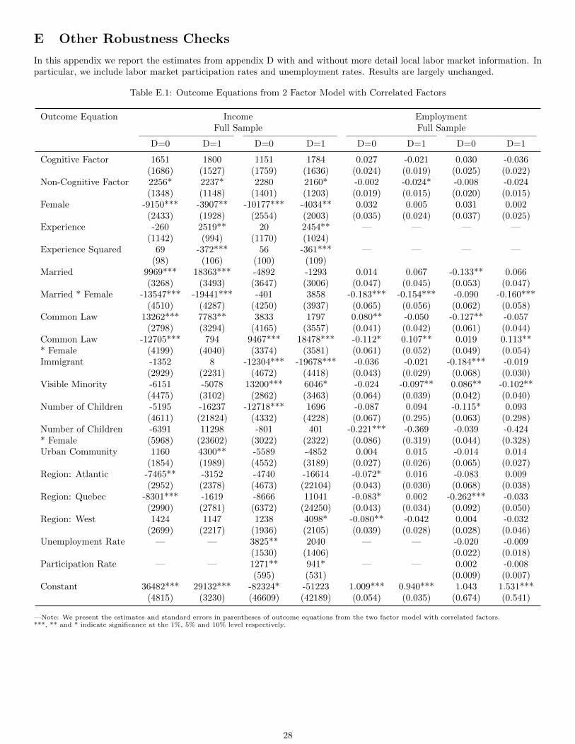
E Other Robustness Checks

In this appendix we report the estimates from appendix D with and without more detail local labor market information. Inparticular, we include labor market participation rates and unemployment rates. Results are largely unchanged.

Table E.1: Outcome Equations from 2 Factor Model with Correlated Factors

Outcome Equation Income EmploymentFull Sample Full Sample

D=0 D=1 D=0 D=1 D=0 D=1 D=0 D=1

Cognitive Factor 1651 1800 1151 1784 0.027 -0.021 0.030 -0.036(1686) (1527) (1759) (1636) (0.024) (0.019) (0.025) (0.022)

Non-Cognitive Factor 2256* 2237* 2280 2160* -0.002 -0.024* -0.008 -0.024(1348) (1148) (1401) (1203) (0.019) (0.015) (0.020) (0.015)

Female -9150*** -3907** -10177*** -4034** 0.032 0.005 0.031 0.002(2433) (1928) (2554) (2003) (0.035) (0.024) (0.037) (0.025)

Experience -260 2519** 20 2454** — — — —(1142) (994) (1170) (1024)

Experience Squared 69 -372*** 56 -361*** — — — —(98) (106) (100) (109)

Married 9969*** 18363*** -4892 -1293 0.014 0.067 -0.133** 0.066(3268) (3493) (3647) (3006) (0.047) (0.045) (0.053) (0.047)

Married * Female -13547*** -19441*** -401 3858 -0.183*** -0.154*** -0.090 -0.160***(4510) (4287) (4250) (3937) (0.065) (0.056) (0.062) (0.058)

Common Law 13262*** 7783** 3833 1797 0.080** -0.050 -0.127** -0.057(2798) (3294) (4165) (3557) (0.041) (0.042) (0.061) (0.044)

Common Law -12705*** 794 9467*** 18478*** -0.112* 0.107** 0.019 0.113*** Female (4199) (4040) (3374) (3581) (0.061) (0.052) (0.049) (0.054)Immigrant -1352 8 -12304*** -19678*** -0.036 -0.021 -0.184*** -0.019

(2929) (2231) (4672) (4418) (0.043) (0.029) (0.068) (0.030)Visible Minority -6151 -5078 13200*** 6046* -0.024 -0.097** 0.086** -0.102**

(4475) (3102) (2862) (3463) (0.064) (0.039) (0.042) (0.040)Number of Children -5195 -16237 -12718*** 1696 -0.087 0.094 -0.115* 0.093

(4611) (21824) (4332) (4228) (0.067) (0.295) (0.063) (0.298)Number of Children -6391 11298 -801 401 -0.221*** -0.369 -0.039 -0.424* Female (5968) (23602) (3022) (2322) (0.086) (0.319) (0.044) (0.328)Urban Community 1160 4300** -5589 -4852 0.004 0.015 -0.014 0.014

(1854) (1989) (4552) (3189) (0.027) (0.026) (0.065) (0.027)Region: Atlantic -7465** -3152 -4740 -16614 -0.072* 0.016 -0.083 0.009

(2952) (2378) (4673) (22104) (0.043) (0.030) (0.068) (0.038)Region: Quebec -8301*** -1619 -8666 11041 -0.083* 0.002 -0.262*** -0.033

(2990) (2781) (6372) (24250) (0.043) (0.034) (0.092) (0.050)Region: West 1424 1147 1238 4098* -0.080** -0.042 0.004 -0.032

(2699) (2217) (1936) (2105) (0.039) (0.028) (0.028) (0.046)Unemployment Rate — — 3825** 2040 — — -0.020 -0.009

(1530) (1406) (0.022) (0.018)Participation Rate — — 1271** 941* — — 0.002 -0.008

(595) (531) (0.009) (0.007)Constant 36482*** 29132*** -82324* -51223 1.009*** 0.940*** 1.043 1.531***

(4815) (3230) (46609) (42189) (0.054) (0.035) (0.674) (0.541)

—Note: We present the estimates and standard errors in parentheses of outcome equations from the two factor model with correlated factors.***, ** and * indicate significance at the 1%, 5% and 10% level respectively.

28

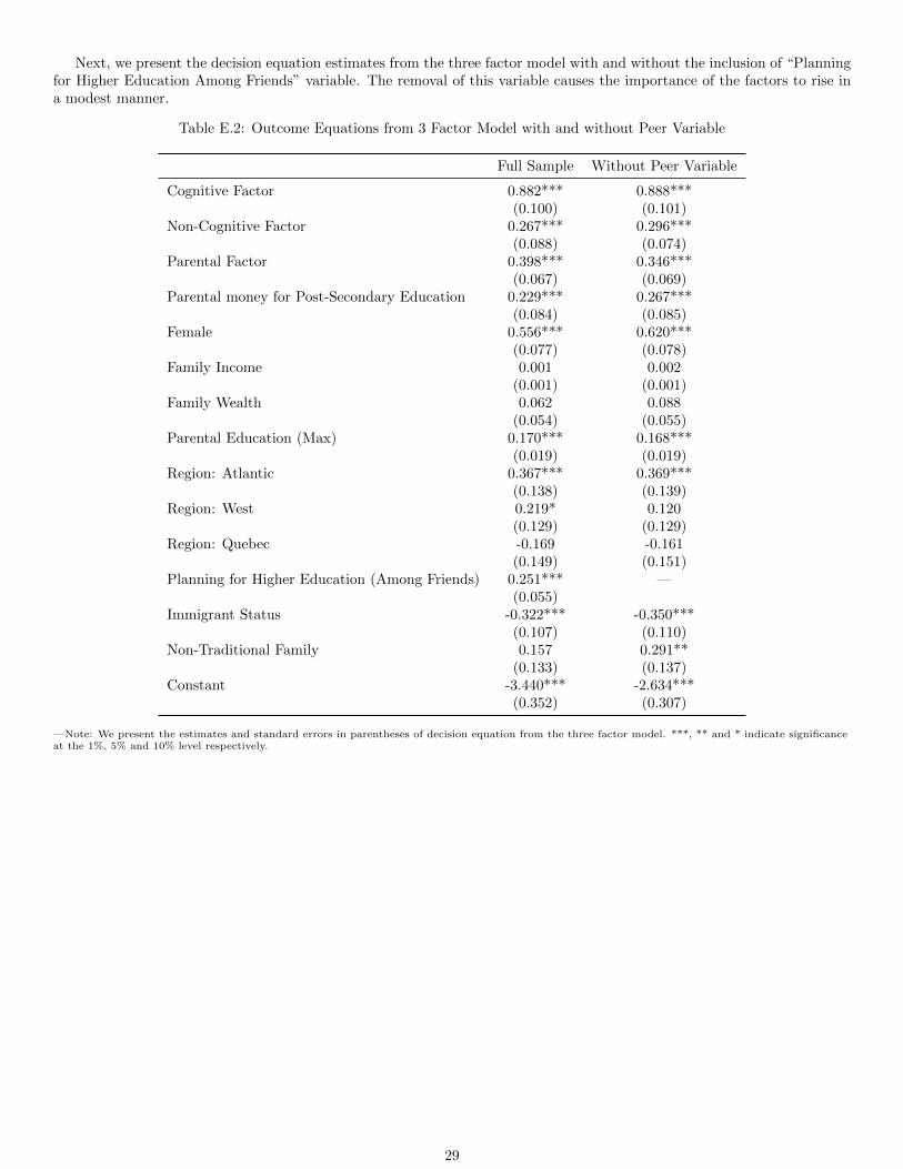
Next, we present the decision equation estimates from the three factor model with and without the inclusion of “Planningfor Higher Education Among Friends” variable. The removal of this variable causes the importance of the factors to rise ina modest manner.

Table E.2: Outcome Equations from 3 Factor Model with and without Peer Variable

Full Sample Without Peer Variable

Cognitive Factor 0.882*** 0.888***(0.100) (0.101)

Non-Cognitive Factor 0.267*** 0.296***(0.088) (0.074)

Parental Factor 0.398*** 0.346***(0.067) (0.069)

Parental money for Post-Secondary Education 0.229*** 0.267***(0.084) (0.085)

Female 0.556*** 0.620***(0.077) (0.078)

Family Income 0.001 0.002(0.001) (0.001)

Family Wealth 0.062 0.088(0.054) (0.055)

Parental Education (Max) 0.170*** 0.168***(0.019) (0.019)

Region: Atlantic 0.367*** 0.369***(0.138) (0.139)

Region: West 0.219* 0.120(0.129) (0.129)

Region: Quebec -0.169 -0.161(0.149) (0.151)

Planning for Higher Education (Among Friends) 0.251*** —(0.055)

Immigrant Status -0.322*** -0.350***(0.107) (0.110)

Non-Traditional Family 0.157 0.291**(0.133) (0.137)

Constant -3.440*** -2.634***(0.352) (0.307)

—Note: We present the estimates and standard errors in parentheses of decision equation from the three factor model. ***, ** and * indicate significanceat the 1%, 5% and 10% level respectively.

29