How Do Massive Black Holes Get Their Gas?
36
Mon. Not. R. Astron. Soc. 000, 000–000 (0000) Printed 11 October 2018 (MN L A T E X style file v2.2) How Do Massive Black Holes Get Their Gas? Philip F. Hopkins 1 * & Eliot Quataert 1 1 Department of Astronomy and Theoretical Astrophysics Center, University of California Berkeley, Berkeley, CA 94720 Submitted to MNRAS, Dec. 14, 2009 ABSTRACT We use multi-scale smoothed particle hydrodynamic simulations to study the inflow of gas from galactic scales (∼ 10kpc) down to . 0.1pc, at which point the gas begins to resemble a traditional, Keplerian accretion disk. The key ingredients of the simulations are gas, stars, black holes (BHs), self-gravity, star formation, and stellar feedback (via a subgrid model); BH feedback is not included. We use ∼ 100 simulations to survey a large parameter space of galaxy properties and subgrid models for the interstellar medium physics. We generate initial conditions for our simulations of galactic nuclei (. 300 pc) using galaxy scale simulations, including both major galaxy mergers and isolated bar-(un)stable disk galaxies. For sufficiently gas-rich, disk-dominated systems, we find that a series of gravitational instabilities generates large accretion rates of up to ∼ 1 - 10 M yr -1 onto the BH (i.e., at . 0.1 pc); this is com- parable to what is needed to fuel the most luminous quasars. The BH accretion rate is highly time variable for a given set of conditions in the galaxy at ∼ kpc. At radii & 10 pc, our sim- ulations resemble the “bars within bars” model of Shlosman et al, but we show that the gas can have a diverse array of morphologies, including spirals, rings, clumps, and bars; the duty cycle of these features is modest, complicating attempts to correlate BH accretion with the morphology of gas in galactic nuclei. At ∼ 1 - 10 pc, the gravitational potential becomes dominated by the BH and bar-like modes are no longer present. However, we show that the gas can become unstable to a standing, eccentric disk or a single-armed spiral mode (m = 1), in which the stars and gas precess at different rates, driving the gas to sub-pc scales (again for sufficiently gas-rich, disk-dominated systems). A proper treatment of this mode requires including star formation and the self-gravity of both the stars and gas (which has not been the case in many previous calculations). Our simulations predict a correlation between the BH accretion rate and the star formation rate at different galactic radii. We find that nuclear star formation is more tightly coupled to AGN activity than the global star formation rate of a galaxy, but a reasonable correlation remains even for the latter. Key words: galaxies: active — quasars: general — galaxies: evolution — cosmology: theory 1 INTRODUCTION The inflow of gas into the central parts of galaxies plays a crit- ical role in galaxy formation, ultimately generating phenomena as diverse as bulges and spheroidal galaxies, starbursts and ultra- luminous infrared galaxies (ULIRGs), nuclear stellar clusters, and accretion onto super-massive black holes (BHs). The discovery, in the past decade, of tight correlations between black hole mass and host spheroid properties including mass (Kormendy & Richstone 1995; Magorrian et al. 1998), velocity dispersion (Ferrarese & Mer- ritt 2000; Gebhardt et al. 2000), and binding energy or potential well depth (Hopkins et al. 2007; Aller & Richstone 2007) implies that these phenomena are tightly coupled. It has long been realized that bright, high-Eddington ratio ac- * E-mail:[email protected] cretion (i.e., a quasar) dominates the accumulation of mass in the supermassive BH population (Soltan 1982; Salucci et al. 1999; Shankar et al. 2004). In order to explain the existence of black holes with masses ∼ 10 9 M, the amount of gas required is comparable to that contained in entire large galaxies. Given the short lifetime of the quasar phase . 10 8 yr (Martini 2004), the processes of interest must deliver a galaxy’s worth of gas to the inner regions of a galaxy on a relatively short timescale. There is also compelling evidence that quasar activity is pre- ceded and/or accompanied by a period of intense star formation in galactic nuclei (Sanders et al. 1988a,b; Dasyra et al. 2007; Kauff- mann et al. 2003). The observed properties of bulges at z ∼ 0 inde- pendently require that dissipative processes (gas inflow) dominate the formation and structure of the inner ∼kpc (Ostriker 1980; Carl- berg 1986; Gunn 1987; Kormendy 1989; Hernquist et al. 1993). Hopkins et al. (2009a,d, 2008a) showed that this inner dissipational c 0000 RAS arXiv:0912.3257v2 [astro-ph.CO] 28 May 2010
Transcript of How Do Massive Black Holes Get Their Gas?
Mon. Not. R. Astron. Soc. 000, 000–000 (0000) Printed 11 October 2018 (MN LATEX style file v2.2)
How Do Massive Black Holes Get Their Gas?
Philip F. Hopkins1∗ & Eliot Quataert11Department of Astronomy and Theoretical Astrophysics Center, University of California Berkeley, Berkeley, CA 94720
Submitted to MNRAS, Dec. 14, 2009
ABSTRACTWe use multi-scale smoothed particle hydrodynamic simulations to study the inflow of gasfrom galactic scales (∼ 10kpc) down to . 0.1pc, at which point the gas begins to resemblea traditional, Keplerian accretion disk. The key ingredients of the simulations are gas, stars,black holes (BHs), self-gravity, star formation, and stellar feedback (via a subgrid model);BH feedback is not included. We use ∼ 100 simulations to survey a large parameter space ofgalaxy properties and subgrid models for the interstellar medium physics. We generate initialconditions for our simulations of galactic nuclei (. 300 pc) using galaxy scale simulations,including both major galaxy mergers and isolated bar-(un)stable disk galaxies. For sufficientlygas-rich, disk-dominated systems, we find that a series of gravitational instabilities generateslarge accretion rates of up to ∼ 1− 10M yr−1 onto the BH (i.e., at . 0.1 pc); this is com-parable to what is needed to fuel the most luminous quasars. The BH accretion rate is highlytime variable for a given set of conditions in the galaxy at ∼ kpc. At radii & 10 pc, our sim-ulations resemble the “bars within bars” model of Shlosman et al, but we show that the gascan have a diverse array of morphologies, including spirals, rings, clumps, and bars; the dutycycle of these features is modest, complicating attempts to correlate BH accretion with themorphology of gas in galactic nuclei. At ∼ 1− 10 pc, the gravitational potential becomesdominated by the BH and bar-like modes are no longer present. However, we show that thegas can become unstable to a standing, eccentric disk or a single-armed spiral mode (m = 1),in which the stars and gas precess at different rates, driving the gas to sub-pc scales (againfor sufficiently gas-rich, disk-dominated systems). A proper treatment of this mode requiresincluding star formation and the self-gravity of both the stars and gas (which has not beenthe case in many previous calculations). Our simulations predict a correlation between theBH accretion rate and the star formation rate at different galactic radii. We find that nuclearstar formation is more tightly coupled to AGN activity than the global star formation rate of agalaxy, but a reasonable correlation remains even for the latter.
Key words: galaxies: active — quasars: general — galaxies: evolution — cosmology: theory
1 INTRODUCTION
The inflow of gas into the central parts of galaxies plays a crit-ical role in galaxy formation, ultimately generating phenomenaas diverse as bulges and spheroidal galaxies, starbursts and ultra-luminous infrared galaxies (ULIRGs), nuclear stellar clusters, andaccretion onto super-massive black holes (BHs). The discovery, inthe past decade, of tight correlations between black hole mass andhost spheroid properties including mass (Kormendy & Richstone1995; Magorrian et al. 1998), velocity dispersion (Ferrarese & Mer-ritt 2000; Gebhardt et al. 2000), and binding energy or potentialwell depth (Hopkins et al. 2007; Aller & Richstone 2007) impliesthat these phenomena are tightly coupled.
It has long been realized that bright, high-Eddington ratio ac-
∗ E-mail:[email protected]
cretion (i.e., a quasar) dominates the accumulation of mass in thesupermassive BH population (Soltan 1982; Salucci et al. 1999;Shankar et al. 2004). In order to explain the existence of black holeswith masses ∼ 109M, the amount of gas required is comparableto that contained in entire large galaxies. Given the short lifetime ofthe quasar phase . 108 yr (Martini 2004), the processes of interestmust deliver a galaxy’s worth of gas to the inner regions of a galaxyon a relatively short timescale.
There is also compelling evidence that quasar activity is pre-ceded and/or accompanied by a period of intense star formation ingalactic nuclei (Sanders et al. 1988a,b; Dasyra et al. 2007; Kauff-mann et al. 2003). The observed properties of bulges at z∼ 0 inde-pendently require that dissipative processes (gas inflow) dominatethe formation and structure of the inner∼kpc (Ostriker 1980; Carl-berg 1986; Gunn 1987; Kormendy 1989; Hernquist et al. 1993).Hopkins et al. (2009a,d, 2008a) showed that this inner dissipational
c© 0000 RAS
arX
iv:0
912.
3257
v2 [
astr
o-ph
.CO
] 2
8 M
ay 2
010

2 Hopkins and Quataert
component can constitute a large fraction∼ 5−30% of the galaxy’smass, with stellar (and at some point probably gas) surface densi-ties reaching ∼ 1011−12 M kpc−2.
On large (galactic) scales, several viable processes for initi-ating such inflows are well-known. Major galaxy-galaxy mergersproduce strong non-axisymmetric disturbances of the constituentgalaxies; such disturbances may also be produced in some mi-nor mergers and/or globally self-gravitating isolated galactic disks.Observationally, major mergers are associated with enhancementsin star formation in ULIRGs, sub-millimeter galaxies, and pairsmore generally (e.g. Sanders & Mirabel 1996; Schweizer 1998; Jo-gee 2006; Dasyra et al. 2006; Woods et al. 2006; Veilleux et al.2009). Numerical simulations of mergers have shown that whensuch events occur in gas-rich galaxies, resonant tidal torques lead torapid inflow of gas into the central ∼kpc (Hernquist 1989; Barnes& Hernquist 1991, 1996). The resulting high gas densities triggerstarbursts (Mihos & Hernquist 1994, 1996), and are presumed tofeed rapid black hole growth. Feedback from the starburst and acentral active galactic nucleus (AGN) may also be important, bothfor regulating the BH’s growth (Di Matteo et al. 2005; Hopkinset al. 2005; DeBuhr et al. 2009; Johansson et al. 2009b) and forshutting down future star formation (Springel et al. 2005a; Johans-son et al. 2009a; see, however, DeBuhr et al. 2009).
However, the physics of how gas is transported from ∼ 1 kpcto much smaller scales remains uncertain (e.g., Goodman 2003).Typically, once gas reaches sub-kpc scales, the large-scale torquesproduced by a merger and/or large-scale bar/spiral become less ef-ficient. In the case of stellar bars or spiral waves, there can even bea “hard” barrier to further inflow in the form of an inner Linbladresonance, if the system has a non-trivial bulge. In mergers, the co-alescence of the two systems generates perturbations on all scales,and so allows gas to move through the resonances, but the pertur-bations relax rapidly on small scales, often before gas can inflow.
Local viscous stresses – which are believed to dominate angu-lar momentum transport near the central BH (e.g., Balbus & Haw-ley 1998) – are inefficient at radii & 0.01− 0.1 pc (e.g., Shlosman& Begelman 1989; Goodman 2003; Thompson et al. 2005). It isin principle possible that some molecular clouds could be scatteredonto very low angular momentum orbits, but even the optimisticfueling rates from this process are generally insufficient to produceluminous quasars (see e.g. Hopkins & Hernquist 2006; Kawakatu& Wada 2008; Nayakshin & King 2007). As a consequence, manymodels invoke some form of gravitational torques (“bars withinbars”; Shlosman et al. 1989) to continue transport to smaller radii.As gas is driven into the central kpc by large-scale torques, it willcool rapidly into a disky structure; if this gas reservoir is massiveenough, the gas will be self-gravitating and thus again vulnerableto global instabilities (e.g., the well-known bar and/or spiral waveinstabilities) that can drive some of the gas to yet smaller radii.
To date, numerical simulations have seen the formation ofsuch secondary bars in some circumstances, such as in adaptivemesh refinement (AMR) simulations of galaxy formation (Wiseet al. 2007; Levine et al. 2008; Escala 2007) or particle-splittingsmoothed particle hydrodynamics (SPH) simulations of some ide-alized systems (Escala et al. 2004; Mayer et al. 2007). These stud-ies have served as a critical “proof of concept.” However, these ex-amples have generally been limited by computational expense tostudying a single system at one instant in its evolution, and thus itis difficult to assess how the sub-pc dynamics depends on the largeparameter space of possible inflow conditions from large radii andgalaxy structural parameters.
Alternatively, some simulations simply take an assumed
small-scale structure and/or fixed inflow rate as an initial/boundarycondition, and study the resulting gas dynamics at small radii (e.g.Schartmann et al. 2009; Dotti et al. 2009; Wada & Norman 2002;Wada et al. 2009). These studies have greatly informed our under-standing of nuclear obscuration on small scales (the “torus”), andthe role of stellar feedback in determining the structure and dy-namics of the gas at these radii; it is, however, unclear how to relatethis small-scale dynamics to the larger-scale properties of the hostgalaxy. This is critical for understanding black hole growth and nu-clear star formation in the broader context of galaxy formation.
Observationally, a long standing puzzle has been that manysystems, especially those with weaker inflows on large scales (e.g.bar or spiral wave-unstable disks with some bulge, as opposed tomajor mergers), exhibit no secondary instabilities at ∼ 0.1−1 kpc– in several cases, torques clearly reverse sign inside these radii(Block et al. 2001; García-Burillo et al. 2005). Whether this isgeneric, or the consequence of a low duty cycle, or the result ofthe large-scale inflows simply being too weak in these cases, is notclear. Moreover, even among systems that do show nuclear asym-metries, and that clearly exhibit enhanced star formation and lu-minous AGN, the observed features at smaller radii are very oftennot traditional bars. Rather, they exhibit a diverse morphology, withspirals quite common, along with nuclear rings, barred rings, occa-sional one or three-armed modes, and some clumpy/irregular struc-tures (Martini & Pogge 1999; Peletier et al. 1999; Knapen et al.2000; Laine et al. 2002; Knapen et al. 2002; Greene et al. 2009).
Even if secondary bars or spirals are present at intermediateradii ∼ 10− 100 pc, it has long been recognized that they willcease to be important at yet smaller scales, when the potential be-comes quasi-Keplerian and the global self-gravity of the gas lessimportant; this occurs as one approaches the BH radius of influ-ence, which is∼ 10pc in typical∼ L∗ galaxies (Athanassoula et al.1983, 2005; Shlosman et al. 1989; Heller et al. 2001; Begelman &Shlosman 2009). Indeed, in previous simulations and most analyticcalculations, the “bars-within-bars” model appears to break downat these scales (see e.g. Jogee 2006, and references therein). How-ever, local angular momentum transport is still very inefficient at∼ 10 pc, and the gas is still locally self-gravitating, and so should beable to form stars rapidly (e.g., Thompson et al. 2005). Understand-ing the physics of inflow through these last few pc, especially in aconsistent model that connects to gas on galactic scales (∼ 10kpc),remains one of the key open questions in our understanding of mas-sive BH growth.
In this paper, we present a suite of multi-scale hydrodynamicsimulations that follow gravitational torques and gas inflow fromthe kpc scales of galaxy-wide events through to < 0.1pc where thematerial begins to form a standard thin accretion disk. These sim-ulations include gas cooling, star formation, and self-gravity; feed-back from supernovae and stellar winds is crudely accounted for viaa subgrid model. In order to isolate the physics of angular momen-tum transport, we do not include BH feedback in our calculations.We systematically survey a large range of galaxy properties (e.g.,gas fraction and bulge to disk ratio) and gas thermodynamics, inorder to understand how these influence the dynamics, inflow rates,and observational properties of gas on small scales in galactic nu-clei (∼ 0.1− 100 pc). Our focus in this paper is on the results ofmost observational interest: what absolute inflow rates, star forma-tion rates, and gas/stellar surface density profiles result from sec-ondary gravitational instabilities? What is their effective duty cy-cle? And what range of observational morphologies are predicted?In a future paper (Paper II) we will present a more detailed compar-ison between our numerical results and analytic models of inflow
c© 0000 RAS, MNRAS 000, 000–000
How Do Massive Black Holes Get Their Gas? 3
and angular momentum transport induced by non-axisymmetric in-stabilities in galactic nuclei.
The remainder of this paper is organized as follows. In § 2 wedescribe our simulation methodology, which consists of two levelsof “re-simulations” using initial conditions motivated by galactic-scale simulations. In § 3 we present an overview of our results andshow how a series of gravitational processes leads to gas transportfrom galactic scales to sub-pc scales. In §4 we quantify the resultinginflow rates and gas properties as a function of time and radius inthe simulations. §5 summarizes the conditions required for globalgravitational instability and significant gas inflow. In § 6 we showhow the physics of accretion induced by gravitational instabilitiesleads to a correlation (with significant scatter) between star for-mation at different radii and BH accretion; we also compare theseresults to observations. In § 7 we summarize our results and discussa number of their implications and several additional observationaltests. Further numerical details and tests of our methodology arediscussed in § A. In § B we show how the subgrid model of theISM we use influences our results.
2 METHODOLOGY
We use a suite of hydrodynamic simulations to study the physicsof gas inflow from ∼ 10kpc to ∼ 0.1pc in galactic nuclei. In or-der to probe the very large range in spatial and mass scales, wecarry out a series of “re-simulations.” First, we simulate the dynam-ics on galaxy scales. Specifically, we use representative examplesof gas-rich galaxy-galaxy merger simulations and isolated, moder-ately bar-unstable disk simulations. These are well-resolved downto ∼ 100− 500pc. We use the conditions at these radii (at severaltimes) as the initial conditions for intermediate-scale re-simulationsof the sub-kpc dynamics. In these re-simulations, the smaller vol-ume is simulated at higher resolution, allowing us to resolve thesubsequent dynamics down to∼ 10pc scales – these re-simulationsapproximate the nearly instantaneous behavior of the gas on sub-kpc scales in response to the conditions at∼kpc set by galaxy-scaledynamics. We then repeat our re-simulation method to follow thedynamics down to sub-pc scales where the gas begins to form astandard accretion disk.
Our re-simulations are not intended to provide an exact re-alization of the small-scale dynamics of the larger-scale simula-tion that motivated the initial conditions of each re-simulation (inthe manner of particle-splitting or adaptive-mesh refinement tech-niques). Rather, our goal is to identify the dominant mechanism(s)of angular momentum transport in galactic nuclei and what param-eters they depend on. This approach clearly has limitations, espe-cially at the outer boundaries of the simulations; however, it alsohas a major advantage. By not requiring the conditions at smallradii to be uniquely set by a larger-scale “parent” simulation, wecan run a series of simulations with otherwise identical conditions(on that scale) but systematically vary one parameter (e.g., gas frac-tion or ISM model) over a large dynamic range. This allows us toidentify the physics and galaxy properties that have the biggest ef-fect on gas inflow in galactic nuclei. As we will show, the diversityof behaviors seen in the simulations, and desire to marginalize overthe uncertain ISM physics, makes such a parameter survey critical.
This methodology is discussed in more detail below. First, wedescribe the physics in our simulations, in particular our treatmentof gas cooling, star formation, and feedback from supernovae andyoung stars (§ 2.1). We then summarize the galaxy-scale simula-tions that are used to motivate the initial conditions for subsequentre-simulations (§ 2.2). The intermediate-scale re-simulations, and
the methodology used to construct their initial conditions, are dis-cussed in § 2.3. Finally, we discuss the nuclear-scale resimulations,which are themselves motivated by the intermediate-scale resimu-lations (§ 2.4).
2.1 Gas Physics, Star Formation, and Stellar Feedback
The simulations were performed with the parallel TreeSPH codeGADGET-3 (Springel 2005), based on a fully conservative formula-tion of smoothed particle hydrodynamics (SPH), which conservesenergy and entropy simultaneously even when smoothing lengthsevolve adaptively (see e.g., Springel & Hernquist 2002; Hernquist1993; O’Shea et al. 2005). The detailed numerical methodologyis described in Springel (2005), Springel & Hernquist (2003), andSpringel et al. (2005b).
The simulations include supermassive black holes (BHs) asadditional collisionless particles at the centers of all progenitorgalaxies. In our calculations the BH’s only dynamical role is viaits gravitational influence on the smallest scales ∼ 1− 10 pc. Inparticular, to cleanly isolate the physics of gas inflow, we do not in-clude the subgrid models for BH accretion and feedback that havebeen used in previous works (e.g., Springel et al. 2005b). Duringa galaxy merger, the BHs in each galactic nucleus are assumed tocoalesce and form a single BH at the center of mass of the systemonce they are within a single SPH smoothing length of one anotherand are moving at a relative speed lower than both the local gassound speed and relative escape velocities.
In our models, stars form from the gas using a prescriptionmotivated by the observed Kennicutt (1998) relation. Specifically,we use a star formation rate per unit volume ρ∗ ∝ ρ3/2 with thenormalization chosen so that a Milky-way like galaxy has a totalstar formation rate of about 1M yr−1.
The precise slope, normalization, and scatter of the Schmidt-Kennicutt relation, and even whether or not such a relation is gen-erally applicable, are somewhat uncertain on the smallest spatialscales we model here. This is especially true when the dynamicaltimes become short relative to the main-sequence stellar lifetime(tdyn ∼ 105 − 106 yr in the smallest regions simulated). Nonethe-less, there is some observational and physical motivation for the“standard” parameters we have adopted, even at high surface den-sities. For the densest star forming galaxies, observational studiesfavor a logarithmic slope' 1.7 for the relation between Σ∗ and Σg
(Bouché et al. 2007), not that different from what our model imple-ments. In addition, Tan et al. (2006) and Krumholz & Tan (2007)show that local observations imply a constant star formation effi-ciency in units of the dynamical time (i.e. ρ∗ ∝ ρ1.5) at all densitiesobserved, n∼ 101−6 cm−3 – the highest gas densities in these stud-ies are comparable to the highest gas densities in our simulations(∼ 108 M of gas inside ∼ 10 pc). Finally, Davies et al. (2007) &Hicks et al. (2009) estimate the star formation rate (SFR) and gassurface densities in AGN on exactly the small scales of interest here(∼ 1−10pc); they find a SFR-density relation continuous with thatimplied at “normal” galaxy densities.
To understand the possible impact of uncertainties in theSchmidt-Kennicutt relation on our conclusions, we have adjustedthe slope d ln ρ∗/dlnρ adopted in our simulations between 1.0−2.0in a small set of test runs, fixing the star formation rate at MW-like surface densities of ' 109 M kpc−2 where the observationalconstraints are tight. This amounts to varying the absolute star for-mation efficiency on the smallest resolved scales by a factor of& 100; qualitatively, this could presumably mimic a wide varietyof different physics associated with stellar feedback and star for-
c© 0000 RAS, MNRAS 000, 000–000
4 Hopkins and Quataert
10-2 100 102 104 106 108 1010
Bulk Average Density n [cm-3]
0
50
100
150
200
250E
ffect
ive
Sou
nd S
peed
cs
[km
s-1]
qeos=1qeos=0.25
qeos=0.125qeos=0
Adiabatic(No Cooling)
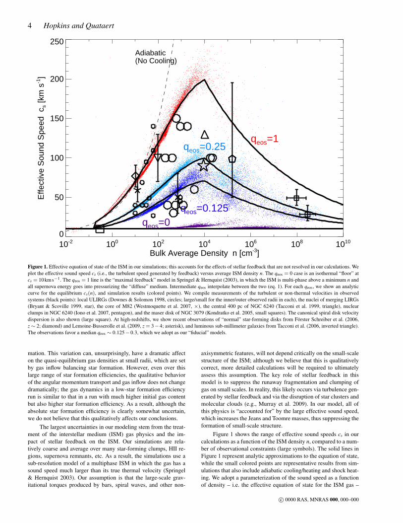
Figure 1. Effective equation of state of the ISM in our simulations; this accounts for the effects of stellar feedback that are not resolved in our calculations. Weplot the effective sound speed cs (i.e., the turbulent speed generated by feedback) versus average ISM density n. The qeos = 0 case is an isothermal “floor” atcs = 10kms−1. The qeos = 1 line is the “maximal feedback” model in Springel & Hernquist (2003), in which the ISM is multi-phase above a minimum n andall supernova energy goes into pressurizing the “diffuse” medium. Intermediate qeos interpolate between the two (eq. 1). For each qeos, we show an analyticcurve for the equilibrium cs(n), and simulation results (colored points). We compile measurements of the turbulent or non-thermal velocities in observedsystems (black points): local ULIRGs (Downes & Solomon 1998, circles; large/small for the inner/outer observed radii in each), the nuclei of merging LIRGs(Bryant & Scoville 1999, star), the core of M82 (Westmoquette et al. 2007, ×), the central 400 pc of NGC 6240 (Tacconi et al. 1999, triangle), nuclearclumps in NGC 6240 (Iono et al. 2007, pentagon), and the maser disk of NGC 3079 (Kondratko et al. 2005, small squares). The canonical spiral disk velocitydispersion is also shown (large square). At high-redshifts, we show recent observations of “normal” star-forming disks from Förster Schreiber et al. (2006,z∼ 2; diamond) and Lemoine-Busserolle et al. (2009, z = 3−4; asterisk), and luminous sub-millimeter galaxies from Tacconi et al. (2006, inverted triangle).The observations favor a median qeos ∼ 0.125−0.3, which we adopt as our “fiducial” models.
mation. This variation can, unsurprisingly, have a dramatic affecton the quasi-equilibrium gas densities at small radii, which are setby gas inflow balancing star formation. However, even over thislarge range of star formation efficiencies, the qualitative behaviorof the angular momentum transport and gas inflow does not changedramatically; the gas dynamics in a low-star formation efficiencyrun is similar to that in a run with much higher initial gas contentbut also higher star formation efficiency. As a result, although theabsolute star formation efficiency is clearly somewhat uncertain,we do not believe that this qualitatively affects our conclusions.
The largest uncertainties in our modeling stem from the treat-ment of the interstellar medium (ISM) gas physics and the im-pact of stellar feedback on the ISM. Our simulations are rela-tively coarse and average over many star-forming clumps, HII re-gions, supernova remnants, etc. As a result, the simulations use asub-resolution model of a multiphase ISM in which the gas has asound speed much larger than its true thermal velocity (Springel& Hernquist 2003). Our assumption is that the large-scale grav-itational torques produced by bars, spiral waves, and other non-
axisymmetric features, will not depend critically on the small-scalestructure of the ISM; although we believe that this is qualitativelycorrect, more detailed calculations will be required to ultimatelyassess this assumption. The key role of stellar feedback in thismodel is to suppress the runaway fragmentation and clumping ofgas on small scales. In reality, this likely occurs via turbulence gen-erated by stellar feedback and via the disruption of star clusters andmolecular clouds (e.g., Murray et al. 2009). In our model, all ofthis physics is “accounted for” by the large effective sound speed,which increases the Jeans and Toomre masses, thus suppressing theformation of small-scale structure.
Figure 1 shows the range of effective sound speeds cs in ourcalculations as a function of the ISM density n, compared to a num-ber of observational constraints (large symbols). The solid lines inFigure 1 represent analytic approximations to the equation of state,while the small colored points are representative results from sim-ulations that also include adiabatic cooling/heating and shock heat-ing. We adopt a parameterization of the sound speed as a functionof density – i.e. the effective equation of state for the ISM gas –
c© 0000 RAS, MNRAS 000, 000–000
How Do Massive Black Holes Get Their Gas? 5
following Springel et al. (2005b); Springel & Hernquist (2005);Robertson et al. (2006a,b). With this model, we can interpolatefreely between two extremes using a parameter qeos. At one ex-treme, the gas has an effective sound speed of 10kms−1, motivatedby, e.g., the observed turbulent velocity in atomic gas in nearbyspirals or the sound speed of low density photo-ionized gas; thisis the “no-feedback” case with qeos = 0. The opposite extreme,qeos = 1, represents the “maximal feedback” sub-resolution modelof Springel et al. (2005b), based on the multiphase ISM modelof McKee & Ostriker (1977); in this case, 100% of the energyfrom supernovae is assumed to stir up the ISM. This equation ofstate is substantially stiffer, with effective sound speeds as high as∼ 200kms−1. Note that at the highest densities, cs begins to de-cline in all of the models (albeit slowly), as the efficiency of starformation asymptotes but cooling rates continue to increase.
Varying qeos between these two extremes amounts to varyingthe effective sound speed of the ISM, with the interpolation
cs =√
qeos c2s [q = 1] + (1−qeos)c2
s [q = 0] . (1)
The resulting sound speeds for qeos = 0.125 and 0.25 are shown inFigure 1; these correspond to more moderate values of cs ∼ 30−100kms−1 for the densities of interest.
Figure 1 compares these models to observations of the turbu-lent (non-thermal) velocities in atomic and molecular gas in a num-ber of systems (large symbols). At low mean densities, n . 0.3−1cm−3, the turbulent velocity in nearby spirals is ∼ 10kms−1.Downes & Solomon (1998) present a detailed study of a numberof luminous local starbursts that have significantly higher meandensities; they decompose the observed molecular line profiles intobulk (e.g., rotation) and turbulent motions. We plot their determi-nation of the mean density and turbulent velocities in each systemat several radii. We also show the results of similar observationsof the core of M82 (Westmoquette et al. 2007), additional nearbyluminous infrared galaxies (Bryant & Scoville 1999), NGC 6240(Tacconi et al. 1999; Iono et al. 2007), and luminous starbursts athigh redshift, z∼ 2−3 (Förster Schreiber et al. 2006; Tacconi et al.2006; Lemoine-Busserolle et al. 2009); at the highest densities, wealso show the random velocities observed in the nuclear maser diskin the nearby Seyfert 2 galaxy NGC3079 (Kondratko et al. 2005).
The observational results in Figure 1 favor models with qeos ≈0.1− 0.3, albeit with significant scatter. We thus take these valuesof qeos as our “standard” choices, although we have carried out nu-merical experiments over the entire range qeos = 0−1. Note that theobservations clearly do not support a simple no-feedback (qeos = 0)model. Within the range qeos ≈ 0.1−0.3, our results on AGN fuel-ing are not particularly sensitive to the precise value of qeos. More-over, the functional form cs(n) is also not crucial: simulations usinga constant cs ' 50kms−1 yield similar results. However, our simu-lations with qeos = 0 and qeos = 1 predict results that are inconsistentwith observations of galactic nuclei – thus, our results themselvesfavor qeos ≈ 0.1−0.3 (see Appendix B).
For the gas densities of interest in this paper, the precise formof the cooling law does not significantly affect our conclusions.This is because the cooling time is almost always much shorterthan the local dynamical time (typical tcool ∼ 10−6−10−4 tdyn). Asa result the "sound speed" of the gas is nearly always pinned tothe subgrid ‘turbulent’ value discussed above (this is why the nu-merical points in Fig. 1 are so close to the analytic models). Thisis true even when the gas is optically thick to the infrared radia-tion produced by dust, as can readily occur in the central ∼ 100pc: the cooling time (diffusion time) is still much less than the dy-namical time in the optically thick limit for the radii that we re-
solve (e.g., Thompson et al. 2005). We have, in fact, experimentedwith alternative cooling rate prescriptions: including or excludingmetal-line cooling, uniformly increasing or decreasing the coolingrate by a factor of ≈ 3, and in the most extreme case, assuminginstantaneous gas cooling (any gas parcel above the cooling flooris assumed to immediately radiate the excess energy in a singletimestep). We do not see any significant changes in our results withthese variations, simply because the gas always cools rapidly inour calculations (in contrast, in regimes such as the α-disk wherethe cooling time is comparable to the dynamical time, the detailsof the cooling function can have a significant effect; see Gammie2001; Nayakshin et al. 2007; Cossins et al. 2009). If the effectiveminimum cs comes from turbulent velocities, then the ÒeffectiveÓcooling time around this SSoor should be given by the turbulent de-cay time, which can be comparable to the dynamical time (Begel-man & Shlosman 2009); this is not included in our calculations. Inthe presence of such an effective cooling time, local gravitationalinstability may lead to tightly wound spirals as opposed to frag-mentation into star-forming clumps. These could be important forangular momentum transport at some radii.
To conclude our discussion of the ISM physics in our sim-ulations, it is important to reiterate that the key role of the sub-resolution sound speed cs is that it determines the local Jeans andToomre criteria, and thus the physical scale on which gravitationalphysics dominates. The Jeans mass for a disk of surface densityΣ and sound speed cs is given by MJ = (π c4
s )/(4G2 Σ). For theouter regions of a galactic disk with Σ∼ 108−109 M kpc−2 andcs ∼ 10kms−1, MJ ∼ 106 M, comparable to that of a molecularcloud; the corresponding Jeans length is tens of pc, comparable tothat of massive molecular cloud complexes in galaxies. Thus oursub-resolution model is effectively averaging over discrete molec-ular clouds and star clusters in galaxies. Large-scale inflows canincrease the surface density in the central regions of galaxies, butcs also rises. In our models with qeos ' 0.1−0.3, the Jeans mass re-mains roughly similar down to ∼pc scales, but as a result the Jeanslength is significantly smaller in galactic nuclei where the ambientdensity is much higher. These physical mass and size-scales mo-tivate the numerical resolution in our simulations; in all cases, weensure that the resolution is sufficient to formally resolve the Jeansmass and length. Higher resolution simulations may be numericallyachievable, but can provide only minimal gains in the “reality” ofthe simulation without a corresponding increase in the sophistica-tion of the ISM model.
2.2 Large Scale Galaxy Mergers and Bars: 100 kpc to 100 pc
Our galaxy-scale simulations motivate the initial conditions chosenfor the smaller-scale re-simulation calculations described in §2.3 &2.4. The galaxy-scale simulations include isolated disks (both glob-ally stable and bar unstable) and galaxy-galaxy mergers. We willultimately focus on a few representative examples, but we chosethose having surveyed a large parameter space. These simulationsand the methodology used for building the initial galaxies are de-scribed in more detail in a series of papers (see e.g. Di Matteo et al.2005; Robertson et al. 2006b; Cox et al. 2006; Younger et al. 2008).We briefly review the key points here.
For each simulation, we generate one or two stable, isolateddisk galaxies, each with an extended dark matter halo with a Hern-quist (1990) profile, an exponential disk of gas and stars, and anoptional stellar bulge. The initial systems are chosen to be consis-tent with the observed baryonic Tully-Fisher relation and estimatedhalo-galaxy mass scaling laws (Bell & de Jong 2001; Kormendy &
c© 0000 RAS, MNRAS 000, 000–000
6 Hopkins and Quataert
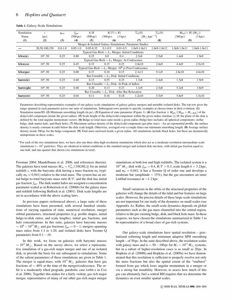
Table 1. Galaxy-Scale Simulations
Simulation ε qeos fgas h/R B/T (< R) Σd(0) Σb(0) Mtot(< R) [M]Name [pc] (500 pc) (500 pc) (300 pc) (1 kpc) [M kpc−2] (300 pc) (1 kpc)
(1) (2) (3) (4) (5) (6) (7) (8) (9)Merger & Isolated Galaxy Simulations: Parameter Studies
— 20,50,100,150 0.0-1.0 0.05-1.0 0.05-0.35 0.1-0.9 0.01-0.5 1.0e9-1.0e11 1.0e9-1.0e12 1.0e8-1.0e11 1.0e8-1.0e11Typical Gas-Rich ∼ L∗ Merger: Initial Conditions
b3ex(ic) 10a, 50 0.25 0.80 0.25 0.8 0.4 2.5e8 2.5e8 1.4e8 1.9e9Typical Gas-Rich ∼ L∗ Merger: At Coalescence
b3ex(co) 10a, 50 0.25 0.45 0.33 0.15 0.25 2.0e10 2.6e9 4.4e9 2.5e10Typical Gas-Rich ∼ L∗ Merger: 108 yr Post-Coalescence
b3ex(po) 10a, 50 0.25 0.08 0.37 0.10 0.15 2.3e11 9.1e9 2.8e10 4.6e10Bar-Unstable ∼ L∗ Disk: Initial Conditions
barex(ic) 10a, 50 0.25 0.40 0.15 0.55 0.35 1.7e8 2.4e8 1.5e8 1.9e9Bar-Unstable ∼ L∗ Disk: At Peak of Inflow
barex(pk) 10a, 50 0.25 0.48 0.20 0.13 0.23 1.1e9 2.5e8 5.2e8 3.8e9Bar-Unstable ∼ L∗ Disk: After Bar Relaxation
barex(re) 10a, 50 0.25 0.04 0.11 0.16 0.18 1.2e10 5.5e9 5.6e9 1.5e10
Parameters describing representative examples of our galaxy-scale simulations of galaxy-galaxy mergers and unstable isolated disks. The top row gives therange spanned in each parameter across our suite of simulations. Subsequent rows pertain to specific examples at chosen times in their evolution. (1)Simulation name/ID. (2) Minimum smoothing length (in pc). (3) Equation of state parameter (Figure 1). (4) Gas fraction ≡Mgas/(Mgas + M∗,disk) of thedisky/cold component (inside the given radius). (5) Scale height of the disky/cold component within the given radius (median |z|/R; the plane of the disk isdefined by the total angular momentum vector). (6) Bulge-to-total mass ratio inside a given radius (bulge here includes all spherical components: stellarbulge, dark matter halo, and black hole). (7) Maximum surface density of the disky/cold component (gas plus stars) – for an exponential profile, the surfacedensity is nearly constant at radii below the disk scale length. Otherwise, averaged over a couple times our minimum smoothing length. (8) Average surfacedensity inside 300 pc for the bulge component. (9) Total mass enclosed inside a given radius. All simulations include black holes, but these are dynamicallyunimportant on these scales.
a For each of the two simulations here, we have also run three ultra high-resolution simulations which also act as a moderate-resolution intermediate-scalesimulations (∼ 107 particles). They are identical in initial conditions to the standard merger and isolated disk run here, with initial gas fraction equal to,one-half, and one-quarter that shown (six simulations in total).
Freeman 2004; Mandelbaum et al. 2006, and references therein).The galaxies have total masses Mvir = V 3
vir/(10GH[z]) for an initialredshift z, with the baryonic disk having a mass fraction md (typi-cally md ' 0.041) relative to the total mass. The system has an ini-tial bulge-to-total baryonic mass ratio B/T , and the disk has initialgas fraction fgas. The dark matter halos are assigned a concentrationparameter scaled as in Robertson et al. (2006b) for the galaxy massand redshift following Bullock et al. (2001). Disk scale lengths areset in accordance with the above scaling laws.
In previous papers (referenced above), a large suite of thesesimulations have been presented, with several hundred simula-tions of varying equation of state, numerical resolution, mergerorbital parameters, structural properties (e.g. profile shapes, initialbulge-to-disk ratios, and scale lengths), initial gas fractions, andhalo concentrations. In this suite, galaxies have baryonic masses∼ 108−1013 M and gas fractions fgas = 0−1; mergers spanningmass ratios from 1:1 to 1:20, and isolated disks have Toomre Qparameters from 0.1−10.
In this work, we focus on galaxies with baryonic masses∼ 1011 M. Based on the survey above, we select a representa-tive simulation of a gas-rich major merger and one of an isolateddisk, to provide the basis for our subsequent re-simulations. Someof the salient parameters of these simulations are given in Table 1.The merger is equal-mass, with 1011 M galaxies that have gasfractions of ∼ 40% at the time of the merger/coalescence. The or-bit is a moderately tilted prograde, parabolic case (orbit e in Coxet al. 2006). Together this makes for a fairly violent, gas rich majormerger, representative of many of our other gas-rich major merger
simulations at both low and high redshifts. The isolated system is a1011 M disk with fgas = 0.4, B/T = 0.3, scale length h = 3.2kpc,and md = 0.041; it has a Toomre Q of order one and develops amoderate bar (amplitude ∼ 15%), but the gas encounters an innerLinblad resonance at ∼1-2 kpc.
Small variations in the orbits or the structural properties of thegalaxies will change the details of the tidal and bar features on largescales. However, the precise details of these large-scale simulationsare not important for our study of the dynamics on small scales (seeAppendix A). Rather, the small-scale dynamics depends on globalparameters such as the gas mass channeled into the central region,relative to the pre-existing bulge, disk, and black hole mass. In theserespects, we have chosen the simulations summarized in Table 1 tobe representative of a broad class of gas-rich systems.
Our galaxy-scale simulations have spatial resolution – grav-itational softening length and minimum adaptive SPH smoothinglength – of 50pc. In the suite described above, the resolution scaleswith galaxy mass and is∼ 50−100pc for M∗ ∼ 1011 M systems,but in a subset of higher-resolution cases is as small as 20pc. InHopkins et al. (2008b) and Hopkins et al. (2009a) we have demon-strated that this resolution is sufficient to properly resolve not onlythe mass fractions but also the spatial extent of the “starburst”formed from gas which loses angular momentum in a merger orvia a strong bar instability. However, to assess how much of thisgas can ultimately fuel a central BH requires that we determine thedynamics on even smaller spatial scales.
c© 0000 RAS, MNRAS 000, 000–000
How Do Massive Black Holes Get Their Gas? 7
2.3 Intermediate Scales: Re-Simulating from 1 kpc to 10 pc
In order to follow the behavior of gas inflow on smaller scales, were-simulate the central regions of interest at higher resolution, in aseries of progressively smaller-scale runs. We begin by selecting anumber of representative outputs from the galaxy-scale simulationsdescribed above, near the peak of activity. We select several snap-shots in the gas-rich merger at key epochs: early close encountersof the two galaxies, just at nuclear coalescence (which is the peakof star formation in the nuclear region), and at the “end” of themerger (roughly ∼ 108 yr after the final coalescence). We also se-lect snapshots typical of isolated, moderately bar-unstable systems,at times where a bar and some inflow has developed; for compar-ison, we also consider a fully stable (pre-bar) galaxy disk. In eachcase, we focus on the central 0.1−1 kpc region, which includes themajority of the gas that has been driven in from larger scales. Someof the representative properties of these snapshots, at these scalesand times, are outlined in Table 1.
Our approach to re-simulating the nuclear region is to usethe larger-scale simulations to motivate the initial conditions of asmaller scale calculation (a “zoom-in” or “re-simulation”). We doso by de-composing the potential, density, and velocity distribu-tions of the gas, stars, and dark matter at a given time in the larger-scale simulation using the basis expansion proposed in Hernquist &Ostriker (1992). This allows us to not only re-construct a smootheddensity profile, but also to include the asymmetric structures fromthe larger-scale simulation (if desired) and to define where the po-tential is noise-dominated.1 From these stellar, gas, and dark matterdistributions, we re-populate the gas and stars in the central regions(the scale we wish to re-simulate; generally out to an outer radius of∼ 1− 2kpc) and use this as the initial condition for a new simula-tion that we run for several local dynamical times. To be conserva-tive, we typically initialize only a small amount of gas in the innerparts of the re-simulation2, since the larger-scale simulation fromwhich the initial condition is drawn has little information about thegas properties on small scales; in Appendix A we show that thesubsequent dynamics does not depend significantly on these detailsof the initial conditions.
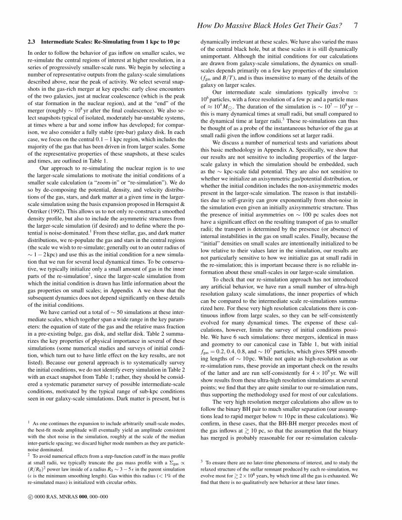
We have carried out a total of ∼ 50 simulations at these inter-mediate scales, which together span a wide range in the key param-eters: the equation of state of the gas and the relative mass fractionin a pre-existing bulge, gas disk, and stellar disk. Table 2 summa-rizes the key properties of physical importance in several of thesesimulations (some numerical studies and surveys of initial condi-tion, which turn out to have little effect on the key results, are notlisted). Because our general approach is to systematically surveythe initial conditions, we do not identify every simulation in Table 2with an exact snapshot from Table 1; rather, they should be consid-ered a systematic parameter survey of possible intermediate-scaleconditions, motivated by the typical range of sub-kpc conditionsseen in our galaxy-scale simulations. Dark matter is present, but is
1 As one continues the expansion to include arbitrarily small-scale modes,the best-fit mode amplitude will eventually yield an amplitude consistentwith the shot noise in the simulation, roughly at the scale of the medianinter-particle spacing; we discard higher mode numbers as they are particle-noise dominated.2 To avoid numerical effects from a step-function cutoff in the mass profileat small radii, we typically truncate the gas mass profile with a Σgas ∝(R/R0)2 power law inside of a radius R0 ∼ 3−5ε in the parent simulation(ε is the minimum smoothing length). Gas within this radius (< 1% of there-simulated mass) is initialized with circular orbits.
dynamically irrelevant at these scales. We have also varied the massof the central black hole, but at these scales it is still dynamicallyunimportant. Although the initial conditions for our calculationsare drawn from galaxy-scale simulations, the dynamics on small-scales depends primarily on a few key properties of the simulation( fgas and B/T ), and is thus insensitive to many of the details of thegalaxy on larger scales.
Our intermediate scale simulations typically involve '106 particles, with a force resolution of a few pc and a particle massof ≈ 104 M. The duration of the simulation is ∼ 107− 108 yr –this is many dynamical times at small radii, but small compared tothe dynamical time at larger radii.3 These re-simulations can thusbe thought of as a probe of the instantaneous behavior of the gas atsmall radii given the inflow conditions set at larger radii.
We discuss a number of numerical tests and variations aboutthis basic methodology in Appendix A. Specifically, we show thatour results are not sensitive to including properties of the larger-scale galaxy in which the simulation should be embedded, suchas the ∼ kpc-scale tidal potential. They are also not sensitive towhether we initialize an axisymmetric gas/potential distribution, orwhether the initial condition includes the non-axisymmetric modespresent in the larger-scale simulation. The reason is that instabili-ties due to self-gravity can grow exponentially from shot-noise inthe simulation even given an initially axisymmetric structure. Thusthe presence of initial asymmetries on ∼ 100 pc scales does nothave a significant effect on the resulting transport of gas to smallerradii; the transport is determined by the presence (or absence) ofinternal instabilities in the gas on small scales. Finally, because the“initial” densities on small scales are intentionally initialized to below relative to their values later in the simulation, our results arenot particularly sensitive to how we initialize gas at small radii inthe re-simulation; this is important because there is no reliable in-formation about these small-scales in our larger-scale simulation.
To check that our re-simulation approach has not introducedany artificial behavior, we have run a small number of ultra-highresolution galaxy scale simulations, the inner properties of whichcan be compared to the intermediate scale re-simulations summa-rized here. For these very high resolution calculations there is con-tinuous inflow from large scales, so they can be self-consistentlyevolved for many dynamical times. The expense of these cal-culations, however, limits the survey of initial conditions possi-ble. We have 6 such simulations: three mergers, identical in massand geometry to our canonical case in Table 1, but with initialfgas = 0.2, 0.4, 0.8, and ∼ 107 particles, which gives SPH smooth-ing lengths of ∼ 10pc. While not quite as high-resolution as ourre-simulation runs, these provide an important check on the resultsof the latter and are run self-consistently for 4× 10⁹ yr. We willshow results from these ultra-high resolution simulations at severalpoints; we find that they are quite similar to our re-simulation runs,thus supporting the methodology used for most of our calculations.
The very high resolution merger calculations also allow us tofollow the binary BH pair to much smaller separation (our assump-tions lead to rapid merger below ≈ 10pc in these calculations). Weconfirm, in these cases, that the BH-BH merger precedes most ofthe gas inflows at & 10 pc, so that the assumption that the binaryhas merged is probably reasonable for our re-simulation calcula-
3 To ensure there are no later-time phenomena of interest, and to study therelaxed structure of the stellar remnant produced by each re-simulation, weevolve most for & 2×10⁸ years, by which time all the gas is exhausted. Wefind that there is no qualitatively new behavior at these later times.
c© 0000 RAS, MNRAS 000, 000–000
8 Hopkins and Quataert
Table 2. Intermediate-Scale Resimulations (∼ 10−1000 pc)
Simulation ε qeos fgas h/R B/T (< R) Σd(0) Σb(0) Mtot(< R) [M]Name [pc] (500 pc) (500 pc) 100 pc 300 pc [M kpc−2] 100 pc 300 pc
(1) (2) (3) (4) (5) (6) (7) (8) (9)If9b5a 1.0 0b,0.175,0.25 0.90 0.30 0.5 0.15 1.0e10 1.1e10 5.4e8 2.9e9If9b5thin 1.0 0.125,0.25 0.90 0.08,0.16 0.4 0.2 1.0e10 1.1e10 5.4e8 2.9e9If9b5res 0.3,1,3,10 0.125 0.90 0.30 0.5 0.15 1.0e10 1.1e10 5.4e8 2.9e9If9b5q 1.0 0,0c,0.125,0.25,0.5,1 0.90 0.30 0.5 0.15 1.0e10 1.1e10 5.4e8 2.9e9Ilowresq 3.0 0,0.25,1 0.95 0.27 0.0 0.0 6.0e10 0.0 1.2e9 4.9e9If1b1late 1.0 0.125 0.096 0.25 0.06 0.03 1.0e11 1.1e10 3.4e9 2.2e10If1b0late 1.0 0.25 0.091 0.28 0.002 0.003 6.0e10 5.0e8 1.3e9 5.3e9If1b0lateLd 2.0 0.25 0.091 0.28 0.005 0.01 6.0e10 5.0e8 7.4e9 8.5e9If3b3mid 1.0 0.125 0.34 0.25 0.3 0.15 3.1e10 2.0e10 1.3e9 7.2e9If3b3midRge 1.0 0.125 0.45,0.20,0.05 0.3,0.5 0.26 0.12 3.6e10 2.0e10 1.5e9 9.2e9If1b3Lmid 1.0 0.25 0.10 0.30 0.07 0.10 6.4e10 1.6e9 1.4e9 5.7e9If1b3LmidLd 2.0 0.25 0.10 0.30 0.15 0.25 6.4e10 1.6e9 8.4e9 1.1e10If5b4mbul 1.0 0.25 0.50 0.24 0.40 0.55 7.4e8 1.9e8 0.3e8 1.3e8If5b8mbul 1.0 0.25 0.50 0.24 0.80 0.90 7.4e8 3.1e9 1.2e8 5.3e8If9b1lowm 1.0 0.25 0.90 0.15 0.03 0.06 6.4e9 1.2e7 1.3e8 5.4e8If3b9dsk 1.0 0.25 0.32 0.22 0.95 0.80 1.6e9 1.1e11 2.1e9 6.2e9If3b9dskLd 2.0 0.25 0.32 0.22 0.71 0.62 1.6e9 1.1e11 8.0e9 9.3e9IfXb2gas 1.0 0.25 0.16,0.32,0.50 0.26 0.16 0.08 3.6e10 1.0e10 1.3e9 7.7e9Inf28b2 1.0 0.20 0.20,0.80 0.25 0.51 0.28 6.3e9 3.0e8 3.6e8 1.7e9Inf28b4 1.0 0.20 0.20,0.80 0.25 0.67 0.43 3.3e9 3.0e8 2.7e8 1.1e9Inf28b6 1.0 0.20 0.20,0.80 0.25 0.78 0.56 3.3e9 6.0e8 4.0e8 1.4e9Inf28b8 1.0 0.20 0.20.0.80 0.25 0.92 0.81 1.0e9 6.0e8 3.4e8 9.5e8Inf2b9 1.0 0.20 0.20 0.25 0.96 0.89 5.2e8 6.0e8 3.2e8 8.6e8Inf28b2hf 0.3 0.125 0.20,0.80 0.25 0.38 0.21 5.5e9 5.0e7 2.3e8 1.1e9Inf8b2hrf 0.3 0.20 0.80 0.25 0.17 0.11 5.5e9 2.5e7 2.2e8 1.1e9Inf28b9hf 0.3 0.125 0.20,0.80 0.25 0.81 0.75 5.5e9 5.0e10 2.1e9 1.1e10
Parameters describing our re-simulations of the 0.01−1 kpc regions from galaxy scale simulations. Parameters separated by commas denotesimulations with otherwise identical initial conditions, re-run with the specified parameter varied. (1) Simulation name/ID. (2) Minimumsmoothing length (in pc). (3) Equation of state parameter (Figure 1). (4) Initial gas fraction of the disky/cold component (inside the given radius).(5) Initial scale height of the disk component (inside the given radius). (6) Initial bulge-to-total mass ratio inside a given radius (again, bulgerefers to all spherical components). (7) Initial maximum surface density of the disky/cold component (gas plus stars). (8) Initial average surfacedensity inside 300 pc for the bulge component (9) Initial total mass enclosed inside a given radius. All simulations include BHs and dark matter,but these are dynamically unimportant on these scales.
a A series of 7 runs testing different means of constructing initial conditions, described in Appendix A.b Isothermal equation of state, but with a large cs = 50kms−1 cooling “floor.”c Cooling allowed down to 100K, i.e. cs = 1kms−1.d Somewhat larger-scale simulation (between “galaxy scale” and standard “intermediate scale”). Instead of B/T (< R) and Mtot(< R) being
evaluated at 100 pc and 300pc, they are here evaluated at 500pc and 1kpc, respectively.e Series where the gas disk profile is allowed to vary independent of the stellar disk profile. The gas has exponential, power-law, and truncated
power-law profiles, with varying concentrations with respect to the disk (for example including an extended gas “reservoir” at a distance ∼ 2times the regular nuclear stellar disk length, with surface density profile Σ∝ R−1).
f Very high-resolution simulations which also act as a moderate-resolution nuclear-scale simulations (2×10⁷ particles; gas particle mass≈ 500M). A series of 6 galaxy-scale runs with very high (∼ 10pc) resolution, used as moderate-resolution intermediate-scale simulations, arealso described in the text.
tions. Moreover, the gas mass at ∼ 10 pc is large (∼ MBH) in themerger simulations. Thus if gas-rich reservoirs indeed drive rapidBH-BH coalescence, the rapid merger of the two BHs should bea reasonable assumption on all of the scales that we simulate (seee.g. Escala et al. 2004; Perets et al. 2007; Mayer et al. 2007; Perets& Alexander 2008; Dotti et al. 2009; Cuadra et al. 2009).
2.4 Nuclear Scales: From 10 pc to 0.1 pc
The characteristic initial scale-lengths of the nuclear disks in ourintermediate scale calculations are ∼ 0.2− 0.5kpc. As we discussin §3, if the gas fraction is sufficiently large, instabilities quicklydevelop that transport material down to ∼ 1−10pc, near the reso-lution limit of our intermediate scale calculations. Material begins
to pile up at these radii because the BH mass dominates the po-tential and the efficiency of large-scale modes decreases at smallradii. In order to understand the dynamics on yet smaller scales, wetherefore repeat our “re-simulation” methodology once more. Theapproach is identical to that described above, but this time usingthe intermediate-scale simulations with resolution of . 10pc as our“parent simulation” from which to motivate the initial conditions.
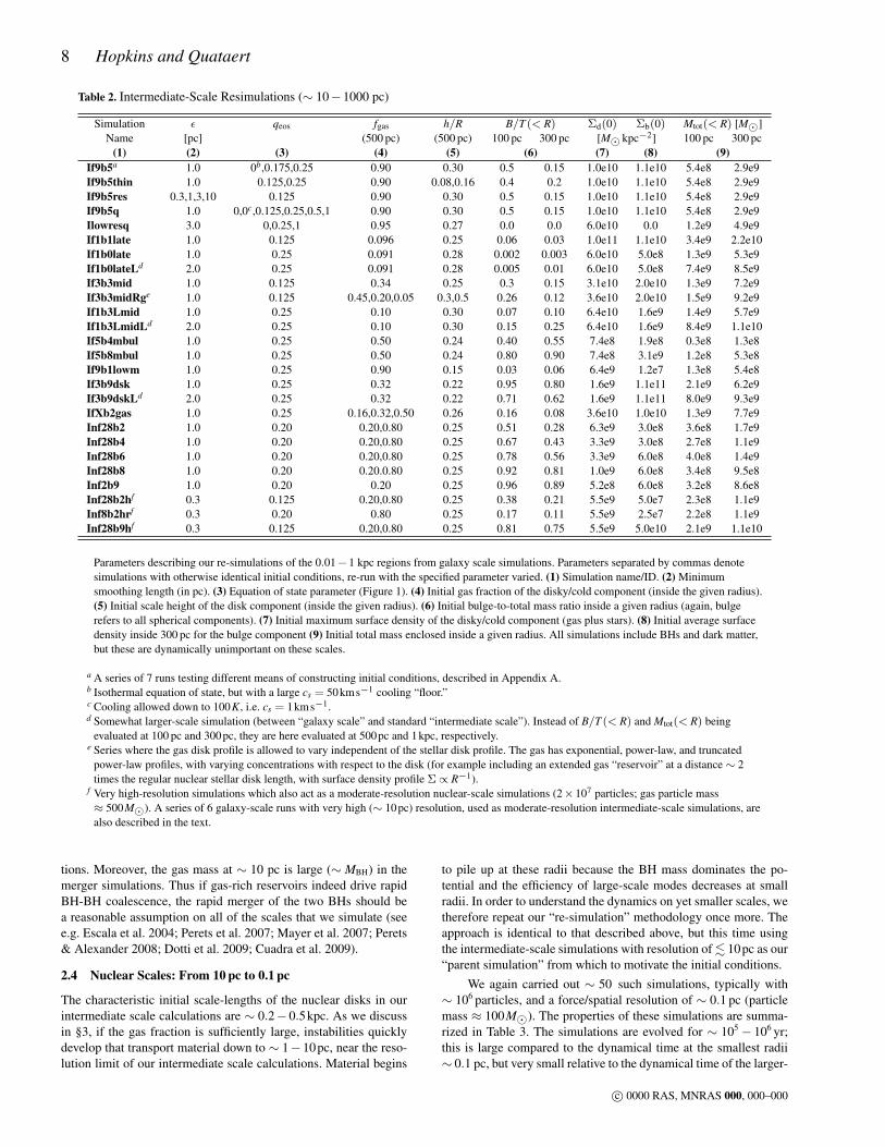
We again carried out ∼ 50 such simulations, typically with∼ 106 particles, and a force/spatial resolution of ∼ 0.1 pc (particlemass ≈ 100M). The properties of these simulations are summa-rized in Table 3. The simulations are evolved for ∼ 105− 106 yr;this is large compared to the dynamical time at the smallest radii∼ 0.1 pc, but very small relative to the dynamical time of the larger-
c© 0000 RAS, MNRAS 000, 000–000
How Do Massive Black Holes Get Their Gas? 9
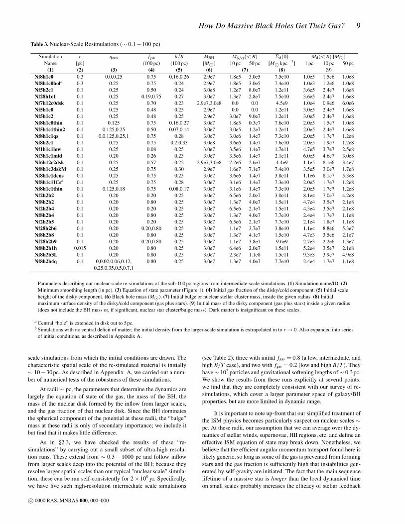
Table 3. Nuclear-Scale Resimulations (∼ 0.1−100 pc)
Simulation ε qeos fgas h/R MBH Mb/cl(< R) Σd(0) Md(< R) [M]Name [pc] (100 pc) (100 pc) [M] 10 pc 50 pc [M kpc−2] 1 pc 10 pc 50 pc
(1) (2) (3) (4) (5) (6) (7) (8) (9)Nf8h1c0 0.3 0.0,0.25 0.75 0.16,0.26 2.9e7 1.8e5 3.0e5 7.5e10 1.0e5 1.5e6 1.0e8Nf8h1c0hola 0.3 0.25 0.75 0.24 2.9e7 1.8e5 3.0e5 7.4e10 1.0e3 1.2e6 1.0e8Nf5h2c1 0.1 0.25 0.50 0.24 3.0e8 1.2e7 8.0e7 1.2e11 3.6e5 2.4e7 1.6e8Nf28h1c1 0.1 0.25 0.19,0.75 0.27 3.0e7 1.3e7 2.8e7 7.5e10 3.6e5 2.4e7 1.6e8Nf7h12c0dsk 0.1 0.25 0.70 0.23 2.9e7,3.0e8 0.0 0.0 4.5e9 1.0e4 0.9e6 6.0e6Nf5h1c0 0.1 0.25 0.48 0.25 2.9e7 0.0 0.0 1.2e11 3.0e5 2.4e7 1.6e8Nf5h1c2 0.1 0.25 0.48 0.25 2.9e7 3.0e7 9.0e7 1.2e11 3.0e5 2.4e7 1.6e8Nf8h1c0thin 0.1 0.125 0.75 0.16,0.27 3.0e7 1.8e5 0.3e7 7.6e10 2.0e5 1.5e7 1.0e8Nf5h1c1thin2 0.1 0.125,0.25 0.50 0.07,0.14 3.0e7 3.0e5 1.2e7 1.2e11 2.0e5 2.4e7 1.6e8Nf8h1c1qs 0.1 0,0.125,0.25,1 0.75 0.28 3.0e7 3.0e6 1.4e7 7.3e10 2.0e5 1.7e7 1.2e8Nf8h2c1 0.1 0.25 0.75 0.2,0.33 3.0e8 3.6e6 1.4e7 7.6e10 2.0e5 1.9e7 1.2e8Nf1h1c1low 0.1 0.25 0.08 0.25 3.0e7 3.5e6 1.4e7 1.7e11 4.7e5 3.7e7 2.5e8Nf3h1c1mid 0.1 0.20 0.26 0.23 3.0e7 3.5e6 1.4e7 2.1e11 6.0e5 4.6e7 3.0e8Nf6h12c2dsk 0.1 0.25 0.57 0.22 2.9e7,3.0e8 7.2e6 2.6e7 4.4e9 1.1e5 8.1e6 3.4e7Nf8h1c3dskM 0.1 0.25 0.75 0.30 2.9e7 1.6e7 7.1e7 7.4e10 3.5e5 3.0e7 1.7e8Nf8h1c1dens 0.1 0.25 0.75 0.25 3.0e7 3.6e6 1.4e7 3.8e11 1.1e6 8.1e7 5.3e8Nf8h1c1ICsb 0.1 0.25 0.75 0.28 3.0e7 3.1e6 1.4e7 7.3e10 2.0e5 1.7e7 1.2e8Nf8h1c1thin 0.1 0.125,0.18 0.75 0.08,0.17 3.0e7 3.1e6 1.4e7 7.3e10 2.0e5 1.7e7 1.2e8Nf2h2b2 0.1 0.20 0.20 0.25 3.0e7 6.5e6 2.0e7 3.0e11 8.1e4 7.0e7 4.2e8Nf8h2b2 0.1 0.20 0.80 0.25 3.0e7 1.3e7 4.0e7 1.5e11 4.7e4 3.5e7 2.1e8Nf2h2b4 0.1 0.20 0.20 0.25 3.0e7 6.5e6 2.1e7 1.5e11 4.3e4 3.5e7 2.1e8Nf8h2b4 0.1 0.20 0.80 0.25 3.0e7 1.3e7 4.0e7 7.7e10 2.4e4 1.7e7 1.1e8Nf2h2b5 0.1 0.20 0.20 0.25 3.0e7 6.5e6 2.1e7 7.7e10 2.1e4 1.8e7 1.1e8Nf28h2b6 0.1 0.20 0.20,0.80 0.25 3.0e7 1.1e7 3.7e7 3.8e10 1.1e4 8.8e6 5.3e7Nf8h2b8 0.1 0.20 0.80 0.25 3.0e7 1.3e7 4.1e7 1.5e10 4.7e3 3.5e6 2.1e7Nf28h2b9 0.1 0.20 0.20,0.80 0.25 3.0e7 1.1e7 3.8e7 9.6e9 2.7e3 2.2e6 1.3e7Nf8h2b1h 0.015 0.20 0.80 0.25 3.0e7 6.4e6 2.0e7 1.5e11 5.2e4 3.5e7 2.1e8Nf8h2b3L 0.1 0.20 0.80 0.25 3.0e7 2.3e7 1.1e8 1.5e11 9.3e3 3.9e7 4.9e8Nf8h2b4q 0.1 0,0.02,0.06,0.12, 0.80 0.25 3.0e7 1.3e7 4.0e7 7.7e10 2.4e4 1.7e7 1.1e8
0.25,0.35,0.5,0.7,1
Parameters describing our nuclear-scale re-simulations of the sub-100 pc regions from intermediate-scale simulations. (1) Simulation name/ID. (2)Minimum smoothing length (in pc). (3) Equation of state parameter (Figure 1). (4) Initial gas fraction of the disky/cold component. (5) Initial scaleheight of the disky component. (6) Black hole mass (M). (7) Initial bulge or nuclear stellar cluster mass, inside the given radius. (8) Initialmaximum surface density of the disky/cold component (gas plus stars). (9) Initial mass of the disky component (gas plus stars) inside a given radius(does not include the BH mass or, if significant, nuclear star cluster/bulge mass). Dark matter is insignificant on these scales.
a Central “hole” is extended in disk out to 5pc.b Simulations with no central deficit of matter; the initial density from the larger-scale simulation is extrapolated in to r→ 0. Also expanded into series
of initial conditions, as described in Appendix A.
scale simulations from which the initial conditions are drawn. Thecharacteristic spatial scale of the re-simulated material is initially∼ 10−30pc. As described in Appendix A, we carried out a num-ber of numerical tests of the robustness of these simulations.
At radii ∼ pc, the parameters that determine the dynamics arelargely the equation of state of the gas, the mass of the BH, themass of the nuclear disk formed by the inflow from larger scales,and the gas fraction of that nuclear disk. Since the BH dominatesthe spherical component of the potential at these radii, the “bulge”mass at these radii is only of secondary importance; we include itbut find that it makes little difference.
As in §2.3, we have checked the results of these “re-simulations” by carrying out a small subset of ultra-high resolu-tion runs. These extend from ∼ 0.3− 1000 pc and follow inflowfrom larger scales deep into the potential of the BH; because theyresolve larger spatial scales than our typical "nuclear scale" simula-tion, these can be run self-consistently for 2× 10⁸ yr. Specifically,we have five such high-resolution intermediate scale simulations
(see Table 2), three with initial fgas = 0.8 (a low, intermediate, andhigh B/T case), and two with fgas = 0.2 (low and high B/T ). Theyhave∼ 107 particles and gravitational softening lengths of∼ 0.3pc.We show the results from these runs explicitly at several points;we find that they are completely consistent with our survey of re-simulations, which cover a larger parameter space of galaxy/BHproperties, but are more limited in dynamic range.
It is important to note up-front that our simplified treatment ofthe ISM physics becomes particularly suspect on nuclear scales ∼pc. At these radii, our assumption that we can average over the dy-namics of stellar winds, supernovae, HII regions, etc. and define aneffective ISM equation of state may break down. Nonetheless, webelieve that the efficient angular momentum transport found here islikely generic, so long as some of the gas is prevented from formingstars and the gas fraction is sufficiently high that instabilities gen-erated by self-gravity are initiated. The fact that the main sequencelifetime of a massive star is longer than the local dynamical timeon small scales probably increases the efficacy of stellar feedback
c© 0000 RAS, MNRAS 000, 000–000
10 Hopkins and Quataert
and decreases the fraction of the gas turned into stars per dynamicaltime (Murray et al. 2009).
At scales 0.1pc, the potential is fully Keplerian and viscousheating is sufficient to stabilize the disk against its own self-gravity(i.e., Q & 1) (Goodman 2003). At these radii, the system begins toapproach a traditional accretion disk. Given the cessation of starformation and the deep potential well of the BH, we assume thatthe inflow rate at ∼ 0.1 pc is a reasonable proxy for the true accre-tion rate onto the BH. Because our simulations are not well-suitedto describe the physics of the disk on scales . 0.1 pc, we do notperform a further “zoom in.”
3 OVERVIEW: FROM KPC TO SUB-PC SCALES
Using the numerical simulations described in §2, we now describehow gas is transported fromkpc scales topc scales. Initially,our discussion is somewhat qualitative; we focus on emphasizingthe key physics at play and our key results. In § 5 we discuss therelevant stability criteria more quantitatively, and outline some spe-cific criteria necessary for “interesting” gas inflow.
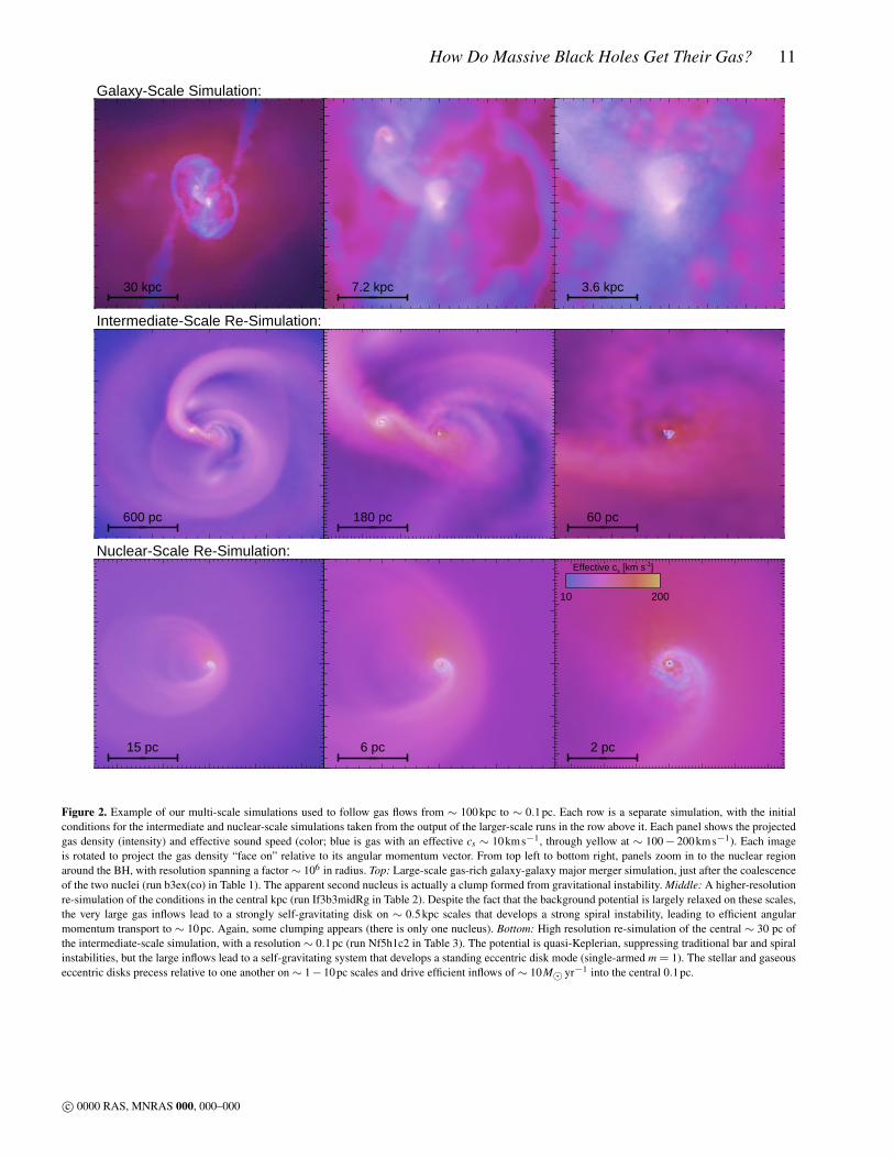
Figure 2 shows an illustrative example of the results of ourre-simulations on various scales. We plot gas surface density maps,with color encoding the gas effective sound speed, from scales of∼ 100kpc to < 1pc. The simulation in this case is a fairly gas-richmajor merger ( fgas ∼ 30−40% at the time of the final coalescence)of two 5× 10¹⁰ M baryonic mass galaxies. The smaller scale re-simulations were carried out just after the coalescence of the twonuclei, which is near the peak of star formation activity, but whenthe system is still quite gas rich. The initial systems had pre-existingbulges of ∼ 1/3 the disk mass and BHs initialized on the MBH−σrelation (∼ 107 M). Each panel is rotated so that the view is closeto “face-on” with respect to the total angular momentum vectorof the gas plotted in the image. Viewed edge-on, much of the gasforms a modestly thin (H/R . 0.3) disky distribution at all radii.
3.1 Large Scales: Mergers and Bars
From ∼ 100kpc to & 100pc, the gas flows are well-resolved byour galaxy-scale simulation. In mergers, the final collision of thetwo galaxies yields strong torques that efficiently cause most of thegas to flow to the center on a timescale approximately equal to afew dynamical times. This process has been described in detail ine.g. Hopkins et al. (2009b), and references therein, but for com-pleteness we briefly summarize the important physics. The sec-ondary/merging galaxy does not directly torque the gas. Rather,the torques on the gas are dominated by local torques from starsoriginally in the same disk as the gas. The merger induces triaxial“sloshes” and bar-like structures in the stars, i.e., non-axisymmetricmodes, supported by radial and/or random orbits. These are alsoinduced in the gas. However, because the gas is dissipational, thegaseous modes slightly lead those in the stars. The stellar distur-bance, being physically close to, trailing, and in near-resonancewith the gas, produces a strong torque that removes angular mo-mentum from the gas and easily dominates the total torque (torquesdirectly from the secondary galaxy, from the primary halo, or hy-drodynamic torques from shocks or internal clump collisions, areall . 10% effects; see e.g. Barnes & Hernquist 1996; Barnes 1998;Hopkins et al. 2009b).
After the two galactic nuclei coalesce, the disturbances in thestellar component of the galaxy relax away in a number of crossingtimes. Until they relax, gas inflows continue. Moreover, the coales-cence of the nuclei completes much more rapidly, in a timescaleclose to a single crossing time, at least in a major merger. Thus, asignificant fraction of the gas inflows can occur in the background
of a rapidly relaxing stellar potential, in the wake of the nuclearcoalescence. This is the stage illustrated in Figure 2.
The gas that loses angular momentum flows in to radii ∼0.5−1kpc (for an ∼ L∗ system), where it participates in a nuclearstarburst and builds a dense central stellar mass concentration, criti-cal for establishing the structural properties and size of the remnantspheroid. At these scales, the system is often gas-dominated for ashort period of time owing to these inflows (provided the mergeris sufficiently gas-rich). However, as the gas forms stars, the cen-tral region will quickly become more stellar-dominated; becausethese stars form out of the gaseous disk, in the relaxing potential— they are not themselves violently relaxed. This is important forthe subsequent evolution of the system because of the presence ofdisk instabilities that would be suppressed by a larger dispersion-supported (spherical) component in the very central region.
The general scenario summarized here can be applied not justto major mergers, but also to minor mergers, fly-by encounters, andeven sufficiently bar-unstable stellar disks. The details will be dif-ferent, but the qualitative steps above, and the exchange of angularmomentum between gas and stars, is robust, ultimately leading toinflow to sub-kpc scales. The subsequent evolution depends largelyhow much material is efficiently channeled to small radii (relativeto the bulge and BH mass), not on how that material gets there.
3.2 Morphology and Gas Transport From 1 kpc to 10 pc
3.2.1 General Behavior
The gas infalling from large radii begins to “pile up” at radii∼ 0.1− 1 kpc, rather than continuously flowing in to yet smallerradii. This is because the torques from the disturbances at largeradii become less efficient at small radii. This happens for threereasons: (1) In the merger context, the stellar perturbation at smallradii relaxes after coalescence, decreasing the efficiency of gas in-flow. (2) The rapid gas inflow implies that the system becomes in-creasingly gas-dominated at radii ∼ 100 pc, even if the initial diskgas fraction is low,∼ 0.1. Because the primary angular momentumsink of the gas is the local stars, when the system becomes locallygas-dominated, angular momentum transfer is actually less efficient(see Hopkins et al. 2009b,f). (3) The gas can encounter the equiv-alent of an inner Linblad resonance. This is especially importantfor unstable gas bars, minor mergers, and disturbances induced byearly passages. For the case of coalescence following major merg-ers, the disturbance is not a single mode, but a series of modes at allscales. As such, there is often no formal inner Linblad resonance orangular momentum barrier (each mode may have such a barrier, butthese are spread over a wide range of scales; there is thus a meansto overcome the barrier associated with any single mode).
Figure 2 shows the outcome of gas pile-up in the centralkpc using an intermediate-scale re-simulation (middle row). In thiscase, the intermediate scale simulation is a high-resolution re-simulation of the larger-scale gas distribution at a given epoch ina gas-rich major merger. The gas density reached from the larger-scale inflows is quite large – ∼ 1010 M worth of gas has formeda disky component with a scale length of 0.3kpc and an averagesurface density of ∼ 1010 M kpc−2. This is a large fraction of thegalaxy mass – larger than the pre-existing bulge within these radii.The small-scale gas disk is therefore strongly self-gravitating. In-deed, we see from Figure 2 that it quickly develops unstable, non-axisymmetric modes.4 This is essentially the “bars within bars”
4 These modes develop almost identically even if we initialize the re-simulation to be perfectly smooth and remove all external tidal forces (see
c© 0000 RAS, MNRAS 000, 000–000
How Do Massive Black Holes Get Their Gas? 11
30 kpc
Galaxy-Scale Simulation:
7.2 kpc
3.6 kpc
600 pc
Intermediate-Scale Re-Simulation:
180 pc
60 pc
15 pc
Nuclear-Scale Re-Simulation:
6 pc
2 pc
Effective cs [km s-1]
10 200
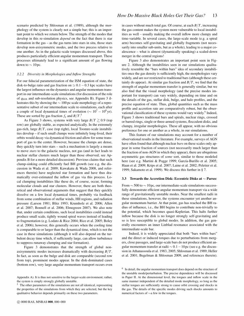
Figure 2. Example of our multi-scale simulations used to follow gas flows from ∼ 100kpc to ∼ 0.1pc. Each row is a separate simulation, with the initialconditions for the intermediate and nuclear-scale simulations taken from the output of the larger-scale runs in the row above it. Each panel shows the projectedgas density (intensity) and effective sound speed (color; blue is gas with an effective cs ∼ 10kms−1, through yellow at ∼ 100− 200kms−1). Each imageis rotated to project the gas density “face on” relative to its angular momentum vector. From top left to bottom right, panels zoom in to the nuclear regionaround the BH, with resolution spanning a factor∼ 106 in radius. Top: Large-scale gas-rich galaxy-galaxy major merger simulation, just after the coalescenceof the two nuclei (run b3ex(co) in Table 1). The apparent second nucleus is actually a clump formed from gravitational instability. Middle: A higher-resolutionre-simulation of the conditions in the central kpc (run If3b3midRg in Table 2). Despite the fact that the background potential is largely relaxed on these scales,the very large gas inflows lead to a strongly self-gravitating disk on ∼ 0.5kpc scales that develops a strong spiral instability, leading to efficient angularmomentum transport to ∼ 10pc. Again, some clumping appears (there is only one nucleus). Bottom: High resolution re-simulation of the central ∼ 30 pc ofthe intermediate-scale simulation, with a resolution ∼ 0.1pc (run Nf5h1c2 in Table 3). The potential is quasi-Keplerian, suppressing traditional bar and spiralinstabilities, but the large inflows lead to a self-gravitating system that develops a standing eccentric disk mode (single-armed m = 1). The stellar and gaseouseccentric disks precess relative to one another on ∼ 1−10pc scales and drive efficient inflows of ∼ 10M yr−1 into the central 0.1pc.
c© 0000 RAS, MNRAS 000, 000–000
12 Hopkins and Quataert
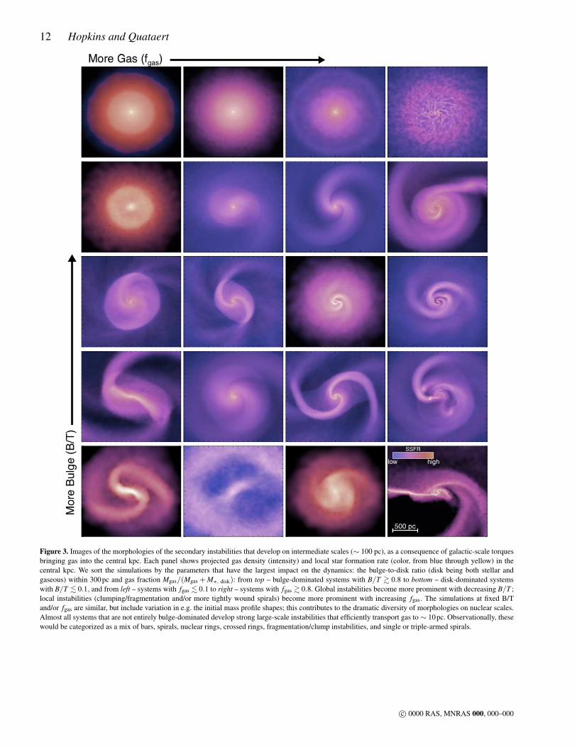
Figure 3. Images of the morphologies of the secondary instabilities that develop on intermediate scales (∼ 100 pc), as a consequence of galactic-scale torquesbringing gas into the central kpc. Each panel shows projected gas density (intensity) and local star formation rate (color, from blue through yellow) in thecentral kpc. We sort the simulations by the parameters that have the largest impact on the dynamics: the bulge-to-disk ratio (disk being both stellar andgaseous) within 300pc and gas fraction Mgas/(Mgas + M∗, disk): from top – bulge-dominated systems with B/T & 0.8 to bottom – disk-dominated systemswith B/T . 0.1, and from left – systems with fgas . 0.1 to right – systems with fgas & 0.8. Global instabilities become more prominent with decreasing B/T ;local instabilities (clumping/fragmentation and/or more tightly wound spirals) become more prominent with increasing fgas. The simulations at fixed B/Tand/or fgas are similar, but include variation in e.g. the initial mass profile shapes; this contributes to the dramatic diversity of morphologies on nuclear scales.Almost all systems that are not entirely bulge-dominated develop strong large-scale instabilities that efficiently transport gas to∼ 10pc. Observationally, thesewould be categorized as a mix of bars, spirals, nuclear rings, crossed rings, fragmentation/clump instabilities, and single or triple-armed spirals.
c© 0000 RAS, MNRAS 000, 000–000
How Do Massive Black Holes Get Their Gas? 13
scenario predicted by Shlosman et al. (1989), although the mor-phology of the system is clearly not a simple bar; this is an impor-tant point to which we return below. The strength of the modes thatdevelop in this re-simulation depend on the fact that there is starformation in the gas – as the gas turns into stars in situ, those starsdevelop non-axisymmetric modes, and the two precess relative toone another. As in the galactic-scale torques discussed above, thisproduces particularly efficient angular momentum transport. Theseprocesses ultimately lead to a significant amount of gas flowingdown to ∼ 10pc.
3.2.2 Diversity in Morphologies and Inflow Strengths
For our fiducial parameterization of the ISM equation of state, thedisk-to-bulge ratio and gas fraction on ' 0.1−0.3 kpc scales havethe largest influence on the dynamics and angular momentum trans-port in our intermediate-scale simulations (for discussion of the roleof qEOS and sub-resolution physics, see Appendix B). Figure 3 il-lustrates this by showing the∼ 100 pc scale morphology of a repre-sentative subset of our intermediate scale re-simulations, each aftera couple of local dynamical times of evolution (∼ 107 − 108 yr).These are sorted by gas fraction fg and B/T .5
As Figure 3 shows, systems with very large B/T & 0.9 (toprow) are globally stable, as expected analytically. In the extremelygas-rich, large B/T , case (top right), local Toomre-scale instabili-ties develop – if such small clumps were infinitely long-lived, theirorbits would decay via dynamical friction and allow for some trans-port of gas to the center. However, because the clumps are dense,they quickly turn into stars – such a mechanism is largely a meansto move stars to the galactic nucleus, not gas (and in fact leads tonuclear stellar clusters much larger than those observed; see Ap-pendix B for a more detailed discussion). Previous claims that suchclump-sinking could efficiently fuel BH growth (see e.g. the dis-cussion in Wada et al. 2009; Kawakatu & Wada 2008, and refer-ences therein) have neglected star formation and have thus dra-matically over-estimated the inflow of gas via this process. Lo-cal clumping instabilities like these do, of course, occur, formingmolecular clouds and star clusters. However, there are both theo-retical and observational arguments that suggest that they quicklydissolve on a few local dynamical times, probably via feedbackfrom some combination of stellar winds, HII regions, and radiationpressure (Larson 1981; Blitz 1993; Krumholz et al. 2006; Allenet al. 2007; Bonnell et al. 2006; Elmegreen 2007). We also notethat, under certain conditions, such local instabilities could insteadproduce small scale, tightly wound spiral waves instead of leadingto fragmentation (e.g. Lodato & Rice 2004; Rice et al. 2005; Boleyet al. 2006); however, this generally occurs when the cooling timeis comparable to or larger than the dynamical time, which is not thecase in these simulations (although it will also depend on the tur-bulent decay time which, if sufficiently large, can allow turbulenceto suppress runaway clumping and star formation).
Figure 3 demonstrates that the strength of global non-axisymmetric modes increases dramatically with decreasing B/T .In fact, as soon as the bulge and disk are comparable (second rowfrom top), prominent modes appear. In the disk-dominated cases(bottom row), very large angular momentum transport occurs even
Appendix A). It is thus not sensitive to the larger-scale environment; rather,the system is simply strongly globally unstable.5 The other parameters of the simulations are not all identical, representingthe properties of the simulations from which they are selected, but the keyqualitative behavior depends primarily on these two parameters.
in cases without much total gas. Of course, at each B/T , increasingthe gas content makes the system more vulnerable to local instabil-ities as well – usually making the overall inflow more clumpy andtime-variable. In several cases, the large-scale mode (e.g. a spiralarm) becomes self-gravitating and globally fragments (not neces-sarily into smaller sub-units, but as a whole), leading to a major co-alescence – what is almost (dynamically speaking) a scaled-downmerger in the central regions!
Figure 3 also demonstrates an important point seen in Fig-ure 2. Although the instabilities seen in our simulations qualita-tively resemble the “bars within bars” idea of secondary instabili-ties once the gas density is sufficiently high, the morphologies varywidely, and are not restricted to traditional bars (although these cer-tainly do appear). At similar gas fraction and B/T , we find that thestrength of angular momentum transfer is generally similar, but wealso find that the visual morphology (and the precise modes im-portant for transport) can vary widely, depending on time and onthe details of the gas, stellar disk, bulge, and halo profiles, and theprecise equation of state. Thus, global quantities such as the massprofile and accretion rate are comparatively robust, but the obser-vational classification of these systems would vary widely.6 Indeed,Figure 3 shows traditional bars and spirals, nuclear rings, crossedor barred rings, single or three-armed systems, flocculent disks, andclumpy, irregular morphologies. These all appear, with no obviouspreference for one or another as a whole, in our simulations.
This feature of our simulations may account for a number ofobservational results in the literature. For example, surveys of AGNhave often found that although nuclear bars on these scales only ap-pear in some fraction of sources (not necessarily much larger thanthe fraction of non-AGN in which they appear), there are ubiquitousasymmetric gas structures of some sort, similar to those modeledhere (see e.g. Martini & Pogge 1999; García-Burillo et al. 2005;Haan et al. 2009; Krips et al. 2007; Laine et al. 2002; Peletier et al.1999; Sakamoto et al. 1999). We discuss this further in § 7.
3.3 Towards the Accretion Disk: Eccentric Disks at ∼ Parsec
From∼ 500 to∼ 10pc, our intermediate-scale simulations success-fully demonstrate efficient angular momentum transport via a widerange of gravitationally unstable modes. Near the smallest radii inthese simulations, however, the systems encounter yet another an-gular momentum barrier. At that point, gas has reached the BH ra-dius of influence, i.e., the BH begins to contribute non-trivially tothe potential, which becomes quasi-Keplerian. This halts furtherinflow because the disk is no longer strongly self-gravitating andso is less susceptible to global modes. In addition, the gas gen-erally encounters an inner Linblad resonance associated with theintermediate-scale bar.
Indeed, it is widely appreciated that both “bars within bars”and the direct or induced torques due to perturbations from merg-ers, close passages, and large-scale bars do not produce efficient an-gular momentum transfer at radii∼ 0.1−10pc (see e.g. the discus-sion in Athanassoula et al. 1983, 2005; Shlosman et al. 1989; Helleret al. 2001; Begelman & Shlosman 2009, and references therein).
6 In detail, the angular momentum transport does depend on the structure ofthe unstable mode/perturbation. The precise dependence will be discussedin Paper II. At the dimensional level, the torques and inflow scale in thesame manner independent of the detailed mode morphology, so long as thestellar torques are sufficiently strong to cause orbit crossing and shocks inthe gas. The details of the specific modes driving such shocks amounts tonumerical factors of ∼a few in the torques.
c© 0000 RAS, MNRAS 000, 000–000
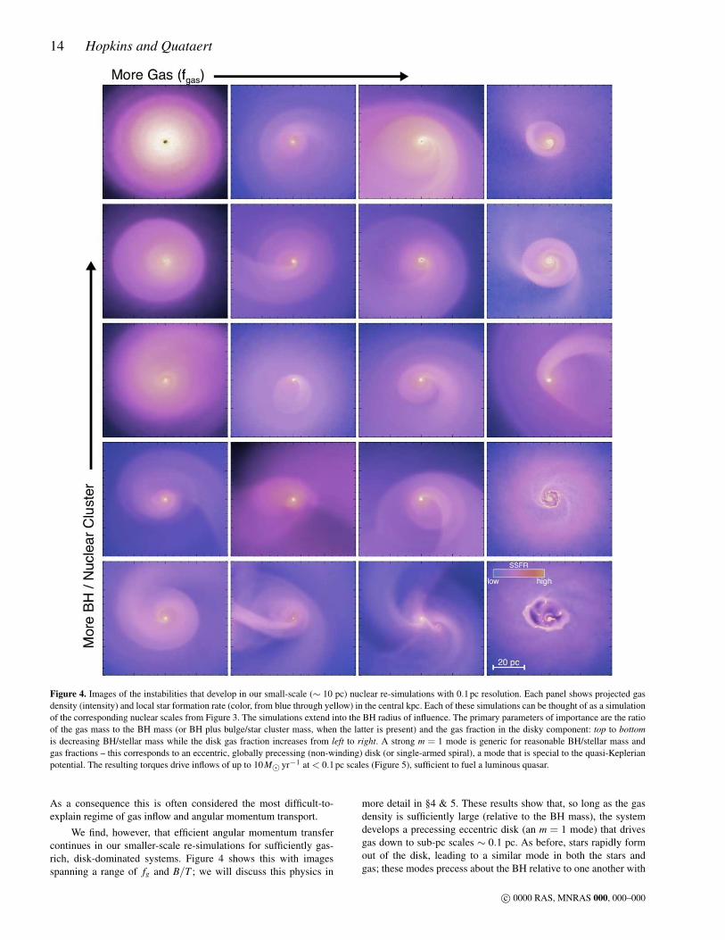
14 Hopkins and Quataert
Figure 4. Images of the instabilities that develop in our small-scale (∼ 10 pc) nuclear re-simulations with 0.1pc resolution. Each panel shows projected gasdensity (intensity) and local star formation rate (color, from blue through yellow) in the central kpc. Each of these simulations can be thought of as a simulationof the corresponding nuclear scales from Figure 3. The simulations extend into the BH radius of influence. The primary parameters of importance are the ratioof the gas mass to the BH mass (or BH plus bulge/star cluster mass, when the latter is present) and the gas fraction in the disky component: top to bottomis decreasing BH/stellar mass while the disk gas fraction increases from left to right. A strong m = 1 mode is generic for reasonable BH/stellar mass andgas fractions – this corresponds to an eccentric, globally precessing (non-winding) disk (or single-armed spiral), a mode that is special to the quasi-Keplerianpotential. The resulting torques drive inflows of up to 10M yr−1 at < 0.1pc scales (Figure 5), sufficient to fuel a luminous quasar.
As a consequence this is often considered the most difficult-to-explain regime of gas inflow and angular momentum transport.
We find, however, that efficient angular momentum transfercontinues in our smaller-scale re-simulations for sufficiently gas-rich, disk-dominated systems. Figure 4 shows this with imagesspanning a range of fg and B/T ; we will discuss this physics in
more detail in §4 & 5. These results show that, so long as the gasdensity is sufficiently large (relative to the BH mass), the systemdevelops a precessing eccentric disk (an m = 1 mode) that drivesgas down to sub-pc scales ∼ 0.1 pc. As before, stars rapidly formout of the disk, leading to a similar mode in both the stars andgas; these modes precess about the BH relative to one another with
c© 0000 RAS, MNRAS 000, 000–000
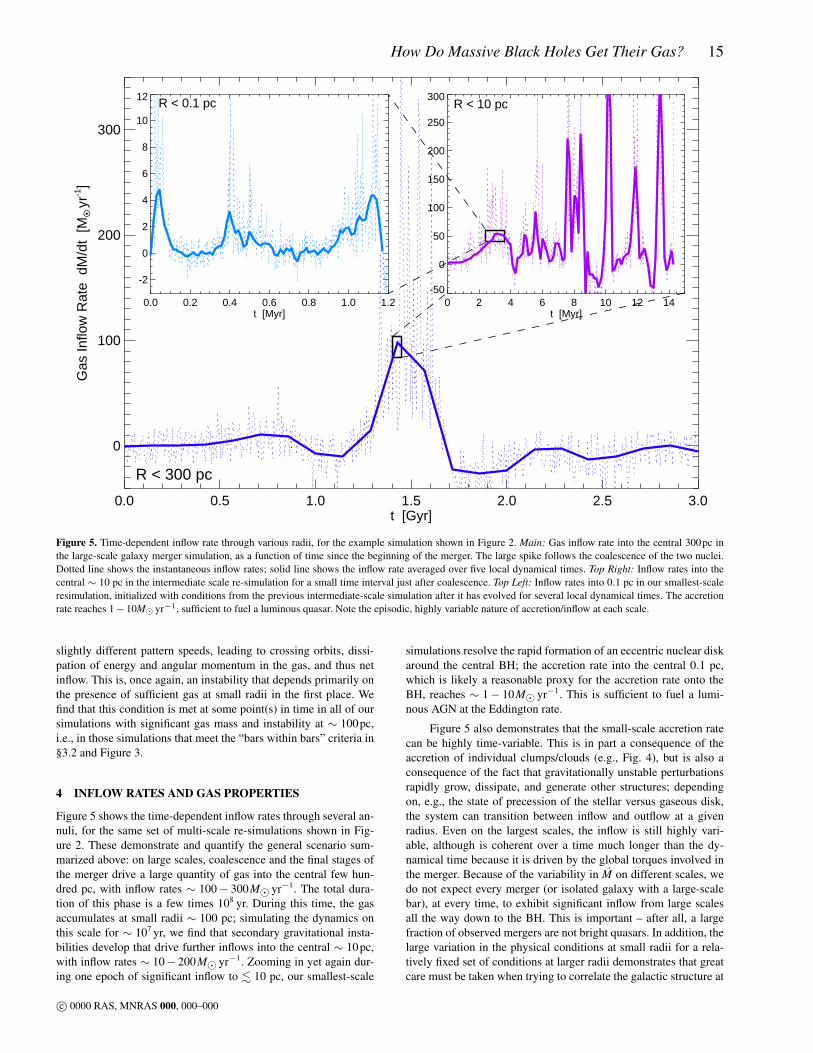
How Do Massive Black Holes Get Their Gas? 15
0.0 0.5 1.0 1.5 2.0 2.5 3.0t [Gyr]
0
100
200
300
Gas
Inflo
w R
ate
dM
/dt
[MO • y
r-1]
R < 300 pc
0 2 4 6 8 10 12 14t [Myr]
-50
0
50
100
150
200
250
300
R < 10 pc
0.0 0.2 0.4 0.6 0.8 1.0 1.2t [Myr]
-2
0
2
4
6
8
10
12
R < 0.1 pc
Figure 5. Time-dependent inflow rate through various radii, for the example simulation shown in Figure 2. Main: Gas inflow rate into the central 300pc inthe large-scale galaxy merger simulation, as a function of time since the beginning of the merger. The large spike follows the coalescence of the two nuclei.Dotted line shows the instantaneous inflow rates; solid line shows the inflow rate averaged over five local dynamical times. Top Right: Inflow rates into thecentral ∼ 10 pc in the intermediate scale re-simulation for a small time interval just after coalescence. Top Left: Inflow rates into 0.1 pc in our smallest-scaleresimulation, initialized with conditions from the previous intermediate-scale simulation after it has evolved for several local dynamical times. The accretionrate reaches 1−10M yr−1, sufficient to fuel a luminous quasar. Note the episodic, highly variable nature of accretion/inflow at each scale.
slightly different pattern speeds, leading to crossing orbits, dissi-pation of energy and angular momentum in the gas, and thus netinflow. This is, once again, an instability that depends primarily onthe presence of sufficient gas at small radii in the first place. Wefind that this condition is met at some point(s) in time in all of oursimulations with significant gas mass and instability at ∼ 100pc,i.e., in those simulations that meet the “bars within bars” criteria in§3.2 and Figure 3.
4 INFLOW RATES AND GAS PROPERTIES
Figure 5 shows the time-dependent inflow rates through several an-nuli, for the same set of multi-scale re-simulations shown in Fig-ure 2. These demonstrate and quantify the general scenario sum-marized above: on large scales, coalescence and the final stages ofthe merger drive a large quantity of gas into the central few hun-dred pc, with inflow rates ∼ 100− 300M yr−1. The total dura-tion of this phase is a few times 108 yr. During this time, the gasaccumulates at small radii ∼ 100 pc; simulating the dynamics onthis scale for ∼ 107 yr, we find that secondary gravitational insta-bilities develop that drive further inflows into the central ∼ 10pc,with inflow rates ∼ 10− 200M yr−1. Zooming in yet again dur-ing one epoch of significant inflow to . 10 pc, our smallest-scale
simulations resolve the rapid formation of an eccentric nuclear diskaround the central BH; the accretion rate into the central 0.1 pc,which is likely a reasonable proxy for the accretion rate onto theBH, reaches ∼ 1− 10M yr−1. This is sufficient to fuel a lumi-nous AGN at the Eddington rate.
Figure 5 also demonstrates that the small-scale accretion ratecan be highly time-variable. This is in part a consequence of theaccretion of individual clumps/clouds (e.g., Fig. 4), but is also aconsequence of the fact that gravitationally unstable perturbationsrapidly grow, dissipate, and generate other structures; dependingon, e.g., the state of precession of the stellar versus gaseous disk,the system can transition between inflow and outflow at a givenradius. Even on the largest scales, the inflow is still highly vari-able, although is coherent over a time much longer than the dy-namical time because it is driven by the global torques involved inthe merger. Because of the variability in M on different scales, wedo not expect every merger (or isolated galaxy with a large-scalebar), at every time, to exhibit significant inflow from large scalesall the way down to the BH. This is important – after all, a largefraction of observed mergers are not bright quasars. In addition, thelarge variation in the physical conditions at small radii for a rela-tively fixed set of conditions at larger radii demonstrates that greatcare must be taken when trying to correlate the galactic structure at
c© 0000 RAS, MNRAS 000, 000–000
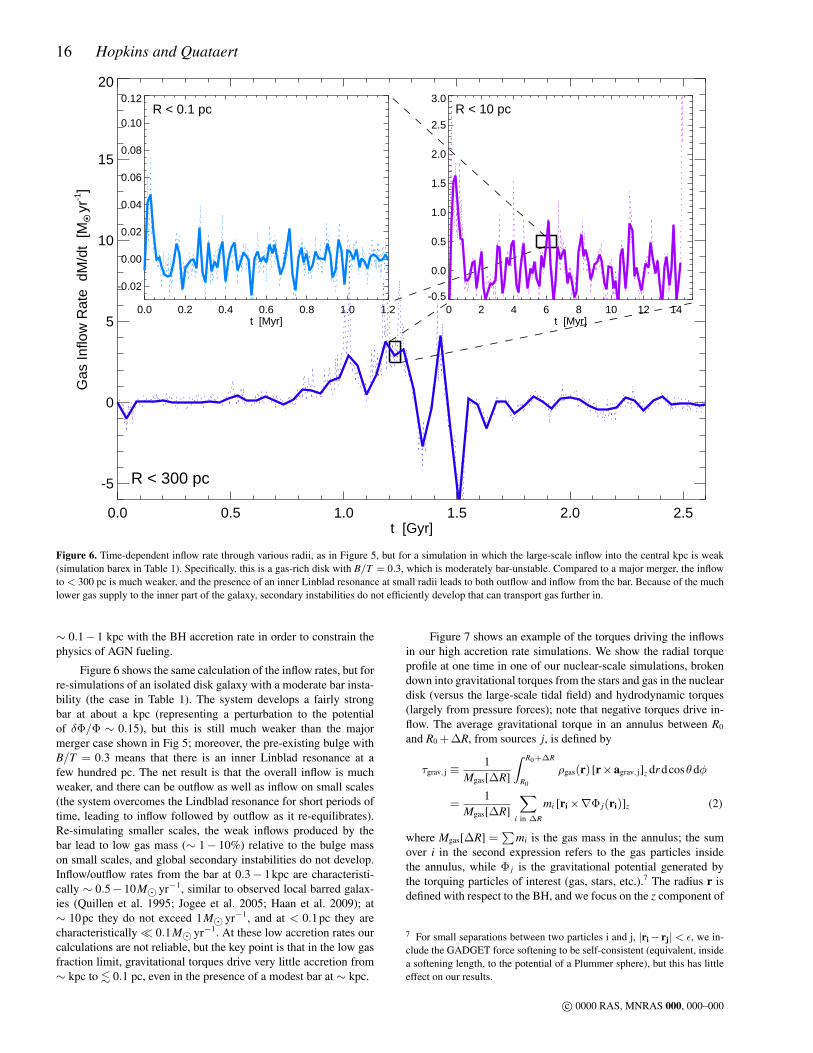
16 Hopkins and Quataert
0.0 0.5 1.0 1.5 2.0 2.5t [Gyr]
-5
0
5
10
15
20G
as In
flow
Rat
e d
M/d
t [M
O • y
r-1]
R < 300 pc
0 2 4 6 8 10 12 14t [Myr]
-0.5
0.0
0.5
1.0
1.5
2.0
2.5
3.0
R < 10 pc
0.0 0.2 0.4 0.6 0.8 1.0 1.2t [Myr]
-0.02
0.00
0.02
0.04
0.06
0.08
0.10
0.12
R < 0.1 pc
Figure 6. Time-dependent inflow rate through various radii, as in Figure 5, but for a simulation in which the large-scale inflow into the central kpc is weak(simulation barex in Table 1). Specifically, this is a gas-rich disk with B/T = 0.3, which is moderately bar-unstable. Compared to a major merger, the inflowto < 300 pc is much weaker, and the presence of an inner Linblad resonance at small radii leads to both outflow and inflow from the bar. Because of the muchlower gas supply to the inner part of the galaxy, secondary instabilities do not efficiently develop that can transport gas further in.
∼ 0.1− 1 kpc with the BH accretion rate in order to constrain thephysics of AGN fueling.
Figure 6 shows the same calculation of the inflow rates, but forre-simulations of an isolated disk galaxy with a moderate bar insta-bility (the case in Table 1). The system develops a fairly strongbar at about a kpc (representing a perturbation to the potentialof δΦ/Φ ∼ 0.15), but this is still much weaker than the majormerger case shown in Fig 5; moreover, the pre-existing bulge withB/T = 0.3 means that there is an inner Linblad resonance at afew hundred pc. The net result is that the overall inflow is muchweaker, and there can be outflow as well as inflow on small scales(the system overcomes the Lindblad resonance for short periods oftime, leading to inflow followed by outflow as it re-equilibrates).Re-simulating smaller scales, the weak inflows produced by thebar lead to low gas mass (∼ 1− 10%) relative to the bulge masson small scales, and global secondary instabilities do not develop.Inflow/outflow rates from the bar at 0.3− 1kpc are characteristi-cally ∼ 0.5− 10M yr−1, similar to observed local barred galax-ies (Quillen et al. 1995; Jogee et al. 2005; Haan et al. 2009); at∼ 10pc they do not exceed 1M yr−1, and at < 0.1pc they arecharacteristically 0.1M yr−1. At these low accretion rates ourcalculations are not reliable, but the key point is that in the low gasfraction limit, gravitational torques drive very little accretion from∼ kpc to . 0.1 pc, even in the presence of a modest bar at ∼ kpc.
Figure 7 shows an example of the torques driving the inflowsin our high accretion rate simulations. We show the radial torqueprofile at one time in one of our nuclear-scale simulations, brokendown into gravitational torques from the stars and gas in the nucleardisk (versus the large-scale tidal field) and hydrodynamic torques(largely from pressure forces); note that negative torques drive in-flow. The average gravitational torque in an annulus between R0
and R0 + ∆R, from sources j, is defined by
τgrav, j ≡1
Mgas[∆R]
∫ R0+∆R
R0
ρgas(r) [r×agrav, j]z dr dcosθdφ
=1
Mgas[∆R]
∑i in ∆R
mi [ri×∇Φ j(ri)]z (2)
where Mgas[∆R] =∑
mi is the gas mass in the annulus; the sumover i in the second expression refers to the gas particles insidethe annulus, while Φ j is the gravitational potential generated bythe torquing particles of interest (gas, stars, etc.).7 The radius r isdefined with respect to the BH, and we focus on the z component of
7 For small separations between two particles i and j, |ri− rj| < ε, we in-clude the GADGET force softening to be self-consistent (equivalent, insidea softening length, to the potential of a Plummer sphere), but this has littleeffect on our results.
c© 0000 RAS, MNRAS 000, 000–000
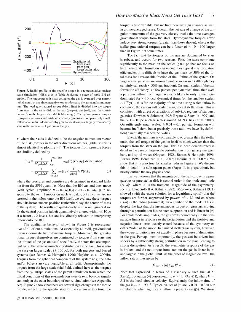
How Do Massive Black Holes Get Their Gas? 17
0.1 1 10 100R [pc]
-400
-200
0
200
⟨τ(R
)⟩ [
km2 s
-2]
Gravitational: from stars from gas large-scale tidesHydrodynamic
Figure 7. Radial profile of the specific torque in a representative nuclearscale simulation (Nf8h1c1qs in Table 3) during a stage of rapid BH ac-cretion. The torque per unit mass acting on the gas is averaged over narrowradial annuli at one time; negative torques decrease the gas angular momen-tum. The total gravitational torque (black line) is divided into the torquefrom stars in the same disk as the gas (purple), gas (red), and the contri-bution from the large-scale tidal field (orange). The hydrodynamic torquesfrom pressure forces and artificial viscosity (green) are comparatively small.Inflow at all radii is dominated by gravitational torques, largely from nearbystars in the same m = 1 pattern as the gas.
τ , where the z axis is defined to be the angular momentum vectorof the disk (torques in the other directions are negligible, so this isalmost identical to plotting |τ |). The torques from pressure forcesare similarly defined by
τP, j ≡1
Mgas[∆R]
∫ R0+∆R
R0
ρgas(r) [r×aP]z dr dcosθdφ
=1
Mgas[∆R]
∑i in ∆R
mi [ri×1
ρ(ri)∇P(ri)]z (3)
where the pressures and densities are determined in standard fash-ion from the SPH quantities. Note that the BH can and does move(with typical amplitude R ∼ 0.1R[Md(< R) ∼ 0.1MBH]) in re-sponse to the m = 1 modes on nuclear scales; but since we are in-terested in the inflow onto the BH itself, we evaluate these torquesabout its instantaneous position (rather than, say, the center-of-massof the system). The results are qualitatively similar in Figure 7 if wefix the central position (albeit quantitatively altered within 10pcat a factor ∼ 2 level), but are less directly relevant to interpretinginflow onto the BH.
The qualitative behavior shown in Figure 7 is representa-tive of all of our simulations. At essentially all radii, gravitationaltorques dominate hydrodynamic torques. Moreover, the gravita-tional torques themselves are dominated by torques from stars, notthe torques of the gas on itself; specifically, the stars that are impor-tant are in the same asymmetric perturbation as the gas. This is alsothe case on larger scales (& 100pc), for both mergers and barredsystems (see Barnes & Hernquist 1996; Hopkins et al. 2009b).Torques from the spherical component of the system (e.g. the haloand/or bulge stars) are negligible at all radii. Unsurprisingly, thetorques from the large-scale tidal field, defined here as the torquesfrom the 100pc scales of the parent simulation from which theinitial conditions of this re-simulation were drawn, become signifi-cant only at the outer boundary of our re-simulation (see AppendixA2). Figure 7 shows that there are several sign changes in the torqueprofile, reflecting the specific state of the system at this time; the
torque is time variable, but we find there are sign changes as wellin a time-averaged sense. Overall, the net rate of change of the an-gular momentum of the gas very closely tracks the time-averagedgravitational torque from the stars. Hydrodynamic torques neverinduce very strong torques (greater than those shown), whereas thestellar gravitational torques can be a factor of ∼ 10− 100 largerthan in Figure 7 at some times.
The fact that the torques on the gas are dominated by starsis robust, and occurs for two reasons. First, the stars contributesignificantly to the mass on the scales & 0.1 pc that we focus onhere (where star formation can occur). For typical star formationefficiencies, it is difficult to have the gas mass 50% of the to-tal mass for a reasonable fraction of the lifetime of the system. Onlarge scales, galaxies are known to not be so gas rich (although theycertainly can reach∼ 50% gas fraction). On small scales, if the starformation efficiency is a few percent per dynamical time, then evena pure gas inflow from larger scales is likely to only remain gas-dominated for ∼ 10 local dynamical times (on the smallest scales,∼ 106 yr) – thus for the majority of the time during which inflow iscontinued, the system will contain a significant stellar mass. This isconsistent with direct observations of sub-kpc regions of starburstgalaxies (Downes & Solomon 1998; Bryant & Scoville 1999) andthe ∼ 1− 10 pc nuclear scales around AGN (Hicks et al. 2009).On sufficiently small scales, . 0.01− 0.1 pc, star formation willbecome inefficient, but at precisely those radii, we have (by defini-tion) essentially reached the α-disk.
Even if the gas mass is comparable to or greater than the stellarmass, the self-torque of the gas on itself is much weaker than thetorques from the stars on the gas. This has been demonstrated indetail in the case of large-scale perturbations from galaxy mergers,bars, and spiral waves (Noguchi 1988; Barnes & Hernquist 1996;Barnes 1998; Berentzen et al. 2007; Hopkins et al. 2009b). Weshow that it is also true for smaller radii in Figure 7. We discussthis in detail in a subsequent paper (Paper II; in preparation), butbriefly outline the key physics here.
It is well-known that the magnitude of the self-torque in a puregaseous or pure stellar disk is second-order in the mode amplitude(∝ |a|2, where |a| is the fractional magnitude of the asymmetry;see e.g. Lynden-Bell & Kalnajs 1972). Moreover, Kalnajs (1971)showed (with the exact solution for a logarithmic spiral) that thetorques are further suppressed by powers of ∼ kR and m, wherek (m) is the radial (azimuthal) wavenumber of the mode. This isdespite the fact that the instantaneous torque on gas/stars movingthrough a perturbation has no such suppression and is linear in |a|.For small mode amplitudes, the gas orbits periodically (in the test-particle limit) in response to the perturbation and the positive andnegative linear terms exactly cancel because of the symmetry oneither “side” of the mode. In a mixed stellar+gas system, however,the two perturbations are not exactly in phase because of dissipationin the gas. Perhaps most importantly, the gas can be driven intoshocks by a sufficiently strong perturbation in the stars, leading tostrong dissipation. As a result, the symmetric response of the gasis broken, and the net torque from stars on the gas is linear in |a|and largest in the global limit. At the order of magnitude level, theinflow rate is thus given by
Mgrav ∼ |a|Σgas R2 Ω. (4)
Note that expressed in terms of a viscosity ν such that M '3πνΣgas, equation (4) corresponds to ν ' (|a|/3π)VcR, where Vc =RΩ is the local circular velocity. Equivalently, the inflow time ofthe gas is∼ |a|−1Ω−1. Typical values of |a| are∼ 0.01−0.3 in oursimulations when significant inflow is present (see §5). We stress
c© 0000 RAS, MNRAS 000, 000–000

18 Hopkins and Quataert
0.1 1
89
101112
log(
Σ) [
MO • k
pc-2]
Nuclear-ScaleRe-Simulation
10 100
Intermediate-ScaleRe-Simulation
GasStars
1000
Galaxy-ScaleSimulation
0.1 1
1
10
100
SF
R(<
R)
[MO • y
r-1]
10 100
1000
0.1 1
1
10
100
dM/d
t [M
O • y
r-1] |a|ΣgasR
2Ω
10 100
1000
0.1 10.01
0.10
1.00
z 0 /
R
10 100
1000
0.1 1R [pc]
0.1
1
10
Qga
s(R
)
10 100R [pc]
1000R [pc]
Figure 8. Properties of representative galactic (right panel), intermediate(middle), and nuclear-scale (left) simulations as a function of radius at asingle time. The simulations are the same as in Figures 2 & 5 and the timechosen corresponds to near the peak of activity, with significant gas inflowto small radii. Note that the initial/boundary conditions for the smaller-scalesimulations were taken from the larger-scale simulations shown, so the re-sults are reasonably continuous at the radial boundaries (despite the factthat these do not represent a self-consistent single simulation). Top: Gasand stellar surface density. Second-from-Top: Enclosed star formation ratein a given radius. Middle: Instantaneous inflow/outflow rate through the an-nulus (black line); note that there are several sign changes as a function ofradius. Also shown is the order of magnitude estimate of the accretion rateproduced by gravitational torques from a non-axisymmetric mode of am-plitude |a|, M ∼ |a|Σgas R2 Ω (dashed red line; § 4). Second-from-Bottom:Scale height z0/R of the gas. Bottom: Toomre Q parameter of the gas.
that, as described above, equation 4 differs fundamentally from thedimensional expectation for self-torques, which is second-order in|a| and suppressed by terms in |kR| and m.
Figure 8 shows a number of properties of our fiducial sim-ulations from Figures 2 & 5, for each of the three spatial scaleswe consider: galactic (∼ kpc), intermediate (∼ 10− 100 pc), and
0.1 1 10 100 1000R [pc]
0.1
1
10
100
[dM
/dt]
/ [ |a
| Σga
sR2 Ω
]
Figure 9. Comparison of the true instantaneous inflow rate in the simula-tions (dM/dt) to the simple dimensional scaling |a|Σgas R2 Ω(R) expectedfor pure gravitational torques, where |a| is the magnitude of the strongestnon-axisymmetric mode at a given radius R (directly measured in the simu-lations; with typical values∼ 0.01−0.3). Each solid line denotes a differentsimulation, with dotted lines showing the radii near the boundaries of ourre-simulations, where the exact profile shape is suspect; colors correspondto initial gas fractions as in Figure 13. Thick dot-dashed lines correspond toultra-high resolution simulations. The simulations are shown during the ac-tive/strong inflow phases, as in Figure 5. The inflow rate in the simulationsis consistent with being produced by gravitational torques over 5 orders ofmagnitude in radius, with relatively little scatter (0.3−0.5dex at all radii).
nuclear (∼ 0.1− 10 pc). We show the stellar and gaseous surfacedensities, the local star formation rate, the gas inflow rate in com-parison to equation 4, and the vertical scale height and Toomre Qof the gas disk. We stress that Figure 8 shows three independentsimulations, but that the smaller-scale simulations were initializedwith properties drawn from the larger-scale simulations; this ex-plains the approximate, but not exact, continuity between the dif-ferent scales. Although Figure 8 is quite instructive, it can also bemisleading to focus on the results of an individual simulation. Thereason is that there is large variation in time and potentially largescatter introduced by modest differences in galaxy properties (dueto, e.g., large-scale fragmentation of a spiral arm biasing the re-sults of a given simulation). For this reason we believe that it isextremely important to consider the statistical properties of a largenumber of simulations that vary the precise initial conditions, gasfraction, bulge to disk ratio, etc. In what follows we now discuss thestatistical properties of the simulations summarized in Tables 1-3.In doing so, we will show a number of Figures that contain the re-sults of many of our simulations. In these Figures, the critical pointto focus on is less the results of any given simulation (which canbe hard to pick out), but rather the ensemble properties of all ofthe simulations (e.g., median, scatter, ...). Recall that the parameterspace spanned by our simulations includes systematic surveys inthe gas fraction, bulge (or BH)-to-disk ratio, and sub-grid equationof state of the gas.
Figure 9 compares the order of magnitude estimate in equa-tion 4 with the true inflow rate in the simulations, as a functionof radius; as in Figure 8, we show the results of simulations onall three of the spatial scales we have simulated, with dotted linesshowing results near the radial boundary of a given calculation. Incalculating Mgrav in equation 4, we approximate |a| using the mag-nitude of the larger of the m = 1 and m = 2 Fourier component ofthe surface density distribution within R (see § 5). The results in
c© 0000 RAS, MNRAS 000, 000–000

How Do Massive Black Holes Get Their Gas? 19
Figure 9 are at the peak of activity for each simulation with sig-nificant inflow, i.e., when M is near-maximum. Modulo a constantnumerical prefactor, the simple scaling in equation (4) works wellover the entire dynamic range of our simulations, with a scatter of∼ 0.3− 0.5dex at any radius. The same equation also works forour ultra-high resolution simulations, which provide a smooth in-terpolation over the boundaries in our typical “re-simulation” cal-culations. The agreement in Figure 9 demonstrates clearly that theinflow rates do not follow the second-order expectations from self-torques in the absence of dissipation. In Paper II, we show that moredetailed modeling of the gas response (accounting for e.g. the de-tails of the perturbation structure) can both predict the overall am-plitude of M in Figure 9 and reduce the scatter to < 0.3dex.
It is also important to note that the inflow rate in equation 4is independent of the sound speed cs, i.e., of the thermodynamicsof the gas. Rather, the inflow rate is determined by the magni-tude of the non-axisymmetric gravitational potential. This is oneof the reasons why we believe that our results are likely to be rel-atively robust, even given the significant uncertainties in the ISMphysics. By contrast, if the transport were dominated by local vis-cous stresses, the accretion rate would be given by Mvisc∼ 3πνΣgas,where ν ' αc2
s/Ω. For large-scale spiral waves, the angular mo-mentum flux associated with the wave corresponds to an effectiveviscosity that is at most ν ∼ csr (Goodman 2003). Comparing thiswith the inflow rate induced by orbit crossing (eq. [4]) highlightsthat the dominant effect of the non-axisymmetric potential is thatthe stellar potential induces crossing orbits in the gas; the directtransport by spiral waves in the gas is smaller by at least a factorof ∼ cs/Vc. We find that in simulations that are initially 100% gas(even those initialized with already-strong mode amplitudes), thetorques tend to remain fairly weak for a few dynamical times un-til the stellar component is non-negligible, at which point strongshocks appear, the stellar and gaseous modes develop a phase-shift,and the inflow rates rise sharply. The pure gas limit is, however,more sensitive to the thermodynamics of the gas and should bestudied in more detail in future work. In our calculations, we findthat it is critical to include stars, gas, and star formation to prop-erly capture inflow in galactic nuclei: it is the interplay betweenthe stars and gas, and the competition between star formation andinflow, that sets the net accretion rate at small radii onto the BH.
Our interpretation and analysis of the inflow rates assumes thatthe gas resides in a self-gravitating, at least modestly thin, disk.To demonstrate this explicitly, Figure 10 shows the vertical scaleheight and Toomre Q parameter of the gas as a function of radius.For each simulation, at a given radius R we determine the scaleheight z0 of the gas by fitting the gas density distribution to a Gaus-sian with dispersion z0 (after projecting to the plane perpendicularto the net angular momentum vector). At large radii, there is scatterowing to the difference between mergers (with sizeable z0/R) andunstable disks. From∼ 1−100pc, z0/R ranges from∼ 0.05−0.25;this is determined by our assumed ISM equation of state, as well askinematic features such as twists and misalignments. At the small-est radii z0/R begins to decrease rapidly because the potential isincreasingly dominated by the BH (the circular velocity increasesbut the maximum sound speeds are finite). Note that, at all radii, theminimum SPH smoothing length hsml . z0, so that the disk thick-ness is at least modestly resolved. Our simulated disks are alwaysreasonably thin because the cooling time is always short comparedto the dynamical time, so that the sound speed in the simulationreliably tracks that of our subgrid model.
Figure 10 also shows the Toomre Q parameter of the gas, de-fined as Q≡ csκ/πGΣd , where κ is the local epicyclic frequency
0.01
0.10
1.00
z 0 /
R0.1 1 10 100 1000
R [pc]
0.1
1
10
Qga
s(R
)
Figure 10. Properties of the gas disks in our simulations. Top: Scale heightz0/R of the gas as a function of radius, for simulations with significant in-flows. Bottom: Toomre Q parameter of the gas. The inflows are robustlyself-gravitating (Q∼ 1) and disky, with z0/R . 0.2. Each solid line denotesa different simulation, with dotted lines showing the radii near the bound-aries of our re-simulations, where the exact profile shape is suspect; colorscorrespond to initial gas fractions as in Figure 13. Thick lines correspondto ultra-high resolution simulations. The range in behavior emphasizes theimportance of a large, statistically representative suite of simulations.
and Σd is the total surface density of the disk (gas plus stars). Withsome scatter, systems largely lie near Q ∼ 1. This is broadly ex-pected for self-regulating disks; in the simulations, Q∼ 1 is a con-sequence of star formation, the assumed stellar feedback, and grav-itational dynamics.
4.1 Gas Density Profiles
Figure 11 shows the gas surface density as a function of time, atdifferent radii, in the high-inflow simulation from Figures 2 & 5.8
Comparison of Figures 5 & 11 clearly indicates that there is a rea-sonable correlation between high inflow rates and high gas surfacedensities at the same radii. However, the correlation is not necessar-ily one-to-one because of the complex time-dependent dynamics onsmall scales. In some cases, the inflow leads the high surface den-sity (e.g., 0.4Myr at 0.1pc or ∼ 2−4Myr at 10pc), in which casethe large M causes the high Σ, rather than the other way around.Occasionally, M and Σ can even be anti-correlated (e.g., at 10Myron 10pc scales).
Figure 12 shows the gas density profiles as a function of ra-dius for our ensemble of simulations (including the individual sim-ulations shown in Figures 5 & 6); for the gas-rich systems in theleft panel, these surface density profiles are at the peak of activ-ity, i.e., when M is relatively high. During these active phases, the
8 Note that for the re-simulations, the density at small r is intentionallyinitialized to be extremely small, but rapidly rises at very early times.
c© 0000 RAS, MNRAS 000, 000–000

20 Hopkins and Quataert
0.0 0.5 1.0 1.5 2.0 2.5 3.0t [Gyr]
6
7
8
9
10
1 kpc300 pc
0 2 4 6 8 10 12 14t [Myr]
9.0
9.5
10.0
10.5
11.0
log(
Σga
s[R
] ) [
MO • k
pc-2]
100 pc30 pc10 pc
0.0 0.2 0.4 0.6 0.8 1.0 1.2t [Myr]
10.5
11.0
11.5
12.0
2 pc0.5 pc0.1 pc
Figure 11. Gas surface density Σgas at different radii as a function of time,for the simulations shown in Figure 5. Top: Large scale galaxy mergersimulation. The box shows the time interval re-simulated in the panel be-low. Middle: Intermediate-scale re-simulation. The box again shows thetime interval for the smaller scale re-simulation. Bottom: Nuclear-scale re-simulation. Comparing with Figure 5, high inflow rates are generally corre-lated with higher local surface densities, but the relation is not one-to-one.
gas reaches a quasi-equilibrium density distribution. For a givenannulus, the net accretion rate to smaller radii is typically a smallfraction of the total rate at which gas is supplied to that annulus.Thus to first approximation, the surface density can be estimatedby considering the competition between star formation and inflowin a given annulus. If the star formation rate surface density scales∝ Σ
3/2gas , as in Kennicutt (1998), then setting the star formation rate
inside some radius equal to the time-averaged inflow rate Min givesan expected 〈Σgas〉 ∝ M2/3
in R−4/3. Given Min ∝ R1/2, which is rea-sonably consistent with Figure 5, this implies Σgas ∝ R−1, similarto the results for the gas rich systems in Figures 11-12 (althoughslightly steeper than the numerical results). There is of course sig-
nificant variation: we show the results from our large suite of simu-lations to emphasize the variation introduced by initial and bound-ary conditions, treatment of star formation and gas physics, etc., butalso to highlight the robust average behavior and the dependence onglobal quantities such as gas fraction and inflow rate at larger radii(see Fig. 13 for the color scheme).
Note that the gas surface densities achieved on small scalescan be extremely large, ∼ 1011 − 1012 M kpc−2 in the central∼ 0.1−10pc; this is comparable to, or even somewhat larger than,the highest-surface density stellar systems known (Hopkins et al.2009e; Hopkins & Hernquist 2009). And it is a factor of ∼ 104
larger than the initial gas surface density at small radii (shownin Fig. 12 for comparison)! Assuming that a significant fractionof the gas eventually turns into stars, the relic stellar density pro-files expected from these gas-rich simulations are similar to the ob-served profiles of nearby “cusp” ellipticals (e.g., Kormendy et al.2009), which are indeed believed to be direct descendants of gas-rich mergers. However, estimating the “final” stellar profile at smallradii, where our simulations are run for only a modest number oflocal dynamical times, requires a careful correction for the effectsof duty cycle, so we defer a more detailed comparison to futurework.
Figure 12 (right panel) also shows the gas surface density pro-files for cases in which the initial large-scale gas inflows are notstrong (e.g., Fig. 6). Most of these simulations represent either ex-tremely gas-poor mergers or (more commonly) systems that areweakly bar unstable or bar unstable but with significant bulge com-ponents (such that bars form efficiently, but inflow stalls at a largeinner Linblad resonance). In such cases, the large-scale dynamicscannot increase the gas density at sub-kpc scales very far above theinitial value of ∼ 108−109 M kpc−2. Without this enhancement,the system is stable against secondary instabilities, and so there islittle gas inflow at small radii (e.g., Fig. 6).
In both the strong and weak inflow cases in Figure 12, oursmall subset of ultra-high resolution simulations (dot-dashed thicklines; 6 galaxy-scale runs that resolve down to ∼ 10pc, and 5intermediate-scale runs that extend to < 1 pc) are fully consistentwith the larger suite of lower resolution re-simulation runs. Thesehigh resolution simulations have continuous inflow from large tosmall radii, and can therefore be run self-consistently for a muchlarger number of dynamical times than our typical resimulation.In spite of this advantage, we find that our resimulation techniqueyields very similar results.
5 CONDITIONS FOR (IN)STABILITY
In the preceding sections, we have presented results for cases inwhich gas inflow from large scales both is, and is not, sufficientto trigger secondary instabilities at small radii, leading to efficientgas inflow down to ∼ 0.1pc. Here we provide a more quantitativeassessment of the conditions under which there is significant inflowof gas to sub-pc scales.
Figure 13 shows how several different measures of the effi-ciency of angular momentum transport and gas inflow depend onthe initial gas fraction fgas and the “bulge” to total ratio B/T – thesame parameters that strongly influence the morphology of the gas(Fig. 3 & 4). We show results for a few different equations of stateqeos (see Fig.1). The quantities we use to define the efficiency of gasinflow are the gas mass within 10 and 0.1pc Mgas(< R) (top panel),the inflow rates within the same radii (middle panel) and the for-mal amplitude of the non-axisymmetric gravitational perturbationsat ∼ 1 and ∼ 100 pc (bottom panel). For the inflow rate (middle
c© 0000 RAS, MNRAS 000, 000–000
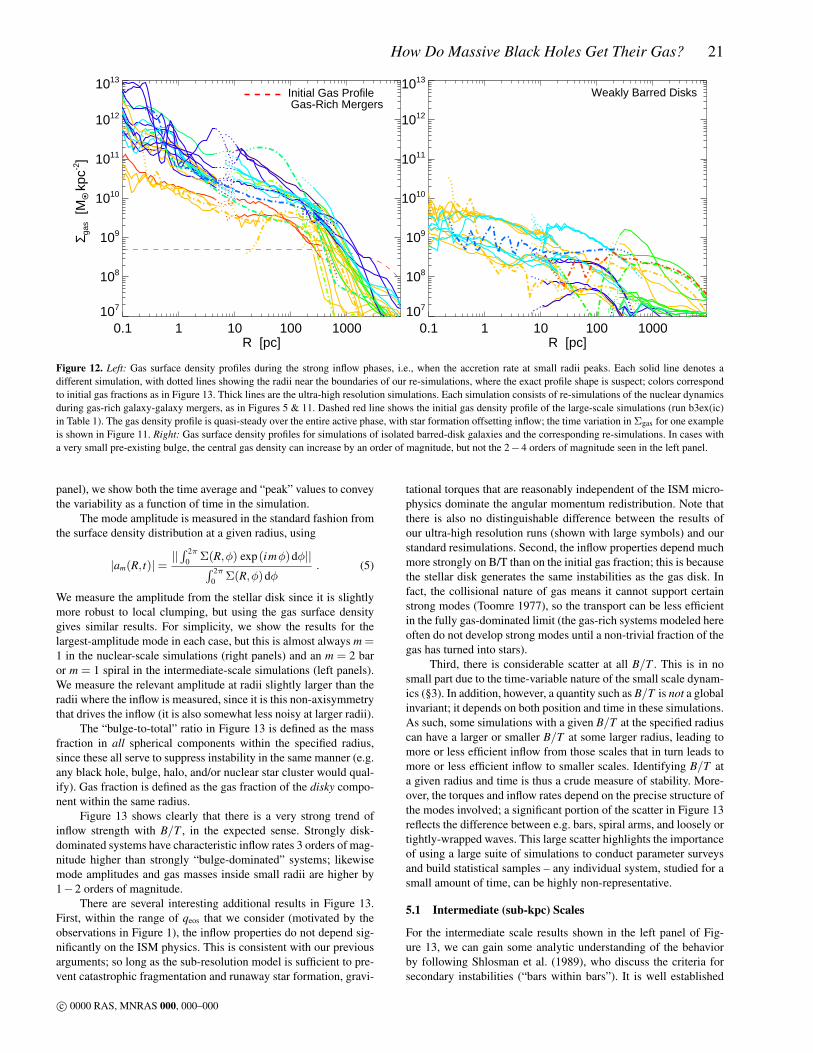
How Do Massive Black Holes Get Their Gas? 21
0.1 1 10 100 1000R [pc]
107
108
109
1010
1011
1012
1013Σ g
as [
MO • k
pc-2]
Gas-Rich MergersInitial Gas Profile
0.1 1 10 100 1000R [pc]
107
108
109
1010
1011
1012
1013
Weakly Barred Disks
Figure 12. Left: Gas surface density profiles during the strong inflow phases, i.e., when the accretion rate at small radii peaks. Each solid line denotes adifferent simulation, with dotted lines showing the radii near the boundaries of our re-simulations, where the exact profile shape is suspect; colors correspondto initial gas fractions as in Figure 13. Thick lines are the ultra-high resolution simulations. Each simulation consists of re-simulations of the nuclear dynamicsduring gas-rich galaxy-galaxy mergers, as in Figures 5 & 11. Dashed red line shows the initial gas density profile of the large-scale simulations (run b3ex(ic)in Table 1). The gas density profile is quasi-steady over the entire active phase, with star formation offsetting inflow; the time variation in Σgas for one exampleis shown in Figure 11. Right: Gas surface density profiles for simulations of isolated barred-disk galaxies and the corresponding re-simulations. In cases witha very small pre-existing bulge, the central gas density can increase by an order of magnitude, but not the 2−4 orders of magnitude seen in the left panel.
panel), we show both the time average and “peak” values to conveythe variability as a function of time in the simulation.
The mode amplitude is measured in the standard fashion fromthe surface density distribution at a given radius, using
|am(R, t)|=||∫ 2π
0 Σ(R,φ) exp(imφ)dφ||∫ 2π0 Σ(R,φ)dφ
. (5)
We measure the amplitude from the stellar disk since it is slightlymore robust to local clumping, but using the gas surface densitygives similar results. For simplicity, we show the results for thelargest-amplitude mode in each case, but this is almost always m =1 in the nuclear-scale simulations (right panels) and an m = 2 baror m = 1 spiral in the intermediate-scale simulations (left panels).We measure the relevant amplitude at radii slightly larger than theradii where the inflow is measured, since it is this non-axisymmetrythat drives the inflow (it is also somewhat less noisy at larger radii).
The “bulge-to-total” ratio in Figure 13 is defined as the massfraction in all spherical components within the specified radius,since these all serve to suppress instability in the same manner (e.g.any black hole, bulge, halo, and/or nuclear star cluster would qual-ify). Gas fraction is defined as the gas fraction of the disky compo-nent within the same radius.
Figure 13 shows clearly that there is a very strong trend ofinflow strength with B/T , in the expected sense. Strongly disk-dominated systems have characteristic inflow rates 3 orders of mag-nitude higher than strongly “bulge-dominated” systems; likewisemode amplitudes and gas masses inside small radii are higher by1−2 orders of magnitude.
There are several interesting additional results in Figure 13.First, within the range of qeos that we consider (motivated by theobservations in Figure 1), the inflow properties do not depend sig-nificantly on the ISM physics. This is consistent with our previousarguments; so long as the sub-resolution model is sufficient to pre-vent catastrophic fragmentation and runaway star formation, gravi-
tational torques that are reasonably independent of the ISM micro-physics dominate the angular momentum redistribution. Note thatthere is also no distinguishable difference between the results ofour ultra-high resolution runs (shown with large symbols) and ourstandard resimulations. Second, the inflow properties depend muchmore strongly on B/T than on the initial gas fraction; this is becausethe stellar disk generates the same instabilities as the gas disk. Infact, the collisional nature of gas means it cannot support certainstrong modes (Toomre 1977), so the transport can be less efficientin the fully gas-dominated limit (the gas-rich systems modeled hereoften do not develop strong modes until a non-trivial fraction of thegas has turned into stars).
Third, there is considerable scatter at all B/T . This is in nosmall part due to the time-variable nature of the small scale dynam-ics (§3). In addition, however, a quantity such as B/T is not a globalinvariant; it depends on both position and time in these simulations.As such, some simulations with a given B/T at the specified radiuscan have a larger or smaller B/T at some larger radius, leading tomore or less efficient inflow from those scales that in turn leads tomore or less efficient inflow to smaller scales. Identifying B/T ata given radius and time is thus a crude measure of stability. More-over, the torques and inflow rates depend on the precise structure ofthe modes involved; a significant portion of the scatter in Figure 13reflects the difference between e.g. bars, spiral arms, and loosely ortightly-wrapped waves. This large scatter highlights the importanceof using a large suite of simulations to conduct parameter surveysand build statistical samples – any individual system, studied for asmall amount of time, can be highly non-representative.
5.1 Intermediate (sub-kpc) Scales
For the intermediate scale results shown in the left panel of Fig-ure 13, we can gain some analytic understanding of the behaviorby following Shlosman et al. (1989), who discuss the criteria forsecondary instabilities (“bars within bars”). It is well established
c© 0000 RAS, MNRAS 000, 000–000

22 Hopkins and Quataert
0.0 0.2 0.4 0.6 0.8 1.0
5
6
7
8
log[
Mga
s(<
R)
] [M
O •]
R < 10 pc
fgas(Initial): 0.1 0.2 0.3 0.5 0.8 0.9
ISM Equation of State:qeos=0.20-0.35qeos=0.125-0.20qeos=0.05-0.125
0.0 0.2 0.4 0.6 0.8 1.0
0.1
1
10
100
Inflo
w d
M/d
t [M
O • y
r-1]
R < 10 pc
0.0 0.2 0.4 0.6 0.8 1.0B/T (<300 pc)
0.01
0.1
1
⟨Mod
e A
mpl
itude
⟩
R < 100 pc
0.0 0.2 0.4 0.6 0.8 1.0
2
3
4
5
R < 0.1 pc
0.0 0.2 0.4 0.6 0.8 1.0
0.01
0.1
1
10
R < 0.1 pc
Time-AveragedMaximum Sampled
0.0 0.2 0.4 0.6 0.8 1.0B/T (<10 pc)
0.01
0.1
R < 1 pc
Figure 13. Inflow strengths as a function of bulge to total ratio (B/T) for several initial gas fractions (colors) and ISM equations of state qeos (symbol type),for a subset of our simulations. Large symbols in each refer to the subset of ultra-high resolution simulations. Top: Total gas mass inside an inner radius of10pc (left; from our intermediate-scale re-simulations) or 0.1pc (right; from our nuclear-scale re-simulations), near the peak of accretion in each simulation.“Bulge” (B) refers to any spherical term in the potential (bulge+halo+black hole). Middle: Gas inflow rate through the relevant inner radius. Solid points denotethe time-averaged inflow rate over the full re-simulation while open points are the maximum seen in any individual snapshot (to give some sense of the dutycycle). Bottom: Amplitude of the dominant non-axisymmetric mode in the stars (generally m = 2 at intermediate scales, m = 1 at nuclear scales), averagedover the peak/strong inflow phase. Inflow properties scale broadly with B/T as expected, but the large scatter and sensitivity to other parameters makes a largeparameter survey critical.
that a self-gravitating disk becomes unstable to large-scale gravi-tational modes roughly when the Ostriker-Peebles criterion is met,i.e., when Trot/|W | > tcrit, where Trot ∼Md V 2
c is the kinetic energyof rotation (in the rotationally supported – i.e. kinematically cold– component), |W | ∼ GM2/R is the potential energy, and tcrit is athreshold value ' 0.15− 0.26, depending on the nature of the in-stability (e.g., Bardeen 1975; Aoki et al. 1979). If a mass fractionfd = 1−B/T is in the disk, the condition for instability generically
becomes
fd > fcrit(tcrit, a/R) (6)
where a is the bulge scale length, R is the disk scale length, and theexact functional form of fcrit depends on the profiles of the disk andbulge. For Kuzmin and Plummer profiles for the disk and bulge,
c© 0000 RAS, MNRAS 000, 000–000

How Do Massive Black Holes Get Their Gas? 23
respectively, we find that this instability criterion becomes
Md[< R]Mb + Md[< R]
>
(3π tcrit
4[1−2 tcrit]Ra
)1/2
(R a) (7)(3π tcrit
16[1 + (a/R)2]
Ra
)(R∼ a) (8)
where Md[< R] is the total (stars + gas) disk mass within R and Mb
is the total bulge mass.If the disky material of interest has a scale-length compara-
ble to that of the bulge (generally true for the intermediate-scalesimulations here), equation (6) simply becomes B/T . 1− tcrit '0.7−0.8. This is reasonably consistent with the fact that the inflowrate and interior gas mass in the intermediate scale simulations inFigure 13 (left column) asymptote for B/T & 0.6−0.7.
Shlosman et al. (1989) show that an initial gas disk must becompressed to at least Rnew/Ri ∼ (1.0− 2.5) f 2
gas/[1 + 0.2(B/T )2]to satisfy equation (6), again for systems in which the disk andbulge initially have similar scale-lengths. For the case of majormergers, we can compare this to Covington et al. (2008) and Hop-kins et al. (2009a,c)’s estimates of how much angular momentumthe gas loses during the merger. These authors find that the gas of-ten inflows until it becomes self-gravitating – as a result, secondarybar instabilities should be ubiquitous. More quantitatively, they findRnew/Ri ≈ fgas/(1+ fgas/ f0) with f0 ≈ 0.2−0.3. Using this, we es-timate that mergers with reasonable gas fractions & 0.3− 0.5 willlead to secondary instabilities and rapid inflow. For isolated diskgalaxies with bars, the critical criterion is whether the inner Lin-blad resonance lies inside or outside of Rnew; this will generally notbe true in low- fgas or high-B/T systems.
5.2 Nuclear (pc) Scales
Inside the radius where the BH begins to dominate the gravita-tional potential, it becomes increasingly difficult for system to beglobally gravitationally unstable in the sense of Trot/|W | > tcrit.Specifically, in the potential of the BH this criterion implies thatthe disk would no longer be unstable inside a radius Rmin ∼10pc(MBH/108 M)1/2 (Σd/1011 M kpc−2)−1/2. This confirmsour earlier claims (e.g., §3.3) that the character of the instabilitiesresponsible for angular momentum transport must change near theBHs radius of influence. Indeed, we see numerically that the trans-port on small scales is dominated by m = 1 modes (e.g., Fig. 4).
A full discussion of the origin of the m = 1 modes is beyondthe scope of this paper; we will present a detailed analytic analy-sis (in simplified BH+disk models) of their structure, growth rates,and pattern speeds in future work (in preparation). We can, how-ever, present a simple analysis indicating how we believe the modesarise. For m = 1 modes, Ω−κ/m→ 0 in a Keplerian potential. It iswell-known that this allows very low frequency (low pattern speedΩp) modes to be present in a Keplerian potential (e.g., Tremaine2001). Moreover, Tremaine (2001) showed that the only modes thatcan be global and exert coherent strong torques over a large dy-namic range in a quasi-Keplerian potential are these m = 1 modes.We find that the modes in the simulations indeed have small Ωp,i.e., ΩpΩ and m = 1, deep in the potential well of the BH. Notethat for a collisionless particle, rather than the stellar+fluid disks ofinterest here, this simply corresponds to a standing elliptical Ke-plerian orbit. Small Ωp/Ω (and wavenumber m = 1) is importantbecause it implies near-resonance conditions at small radii; this al-lows the stars to produce strong torques on the gas, which drives or-bit crossings, shocks, and angular momentum loss, even when themass of the disk at small radii is much less than the BH mass (seee.g. Chang et al. 2007). Following Tremaine (2001) and expanding
the equations of motion for a linear mode in a nearly-Keplerian po-tential (in the WKB limit) it is straightforward to show that themagnitude of the induced velocities (δv/Vc) from a given modescale as δv/Vc ∼ (δΣ/Σ)Md(< R)/MBH = |a|Md(< R)/MBH forall m 6= 1; for m = 1, however, δv/Vc ∼ |a|. In other words, the con-ventional wisdom that torques from global modes are strongly sup-pressed in the spherical potential of a BH is generally true, but theresonance condition that κ ' Ω in Keplerian potentials allows forlarge coherent eccentricities, self-gravitating collective effects, andtorques from m = 1 modes at arbitrarily small disk-to-BH masses.As a result, although we certainly see higher-m modes in our small-scale simulations, the global structure is almost always dominatedby a coherent global m = 1 eccentric disk.
However, Tremaine (2001) also showed that slow modes withpattern speeds Ωp Ω, are linearly stable in quasi-Keplerian po-tentials. How, then, do these modes arise in the simulations? Tostart, we consider the dispersion relation for linear waves in theWKB limit (see e.g. Lau & Bertin 1978), which is given by(ω−mΩ
Ω
)2= 1 +ν−2 fdA
(|kr|2 + m2
)1/2+ A
(|kh|2 +
m2h2
r2
)(9)
where
fd ≡πΣd R2
Menc(< R)≈ Md(< R)
Mtot(< R), (10)
A = 1 +2m2(3−ν)
(ν+ 1)(|kr|2 + m2), (11)
ν ≡ 1 + 2∂ lnVc
∂ lnR≈ dlnMenc(< R)
dlnR, (12)
and h = cs/Ω is the disk thickness. We now consider the limit ofequation (9) such that kr is modest. Of course, our analytic treat-ment of such quasi-global gravitational modes should be consid-ered with due caution, as the WKB approximation necessary to de-rive the dispersion relation is not justified. But this neverthelesspoints towards the conditions under which global gravitational in-stability may be present.9 In this limit, equation (9) will have grow-ing modes if the right-hand side is negative, which for a cold disk(h r) requires
fd >1
2m(1 +ν)2
7−ν . (13)
As ν → 0, i.e., as the potential becomes Keplerian, equation 13suggests that m = 1 modes can become unstable when fd & 0.1.This is consistent with the fact that we find the m = 1 modes atnearly all B/T (Fig. 13). Equation 13 also allows for the instabilityof higher-m modes, but these cannot exert coherent strong torqueson the gas, nor can they propagate efficiently to small radii, so theydo not dominate the structure or inflows we see in our simulations.
Because the disk in general will have more mass at large radii,any instability will grow outside-in; for massive disks, the most-unstable point is where Md(< R)∼ 0.5−1MBH ( fd ∼ 1/3−1/2).
9 Note also that equation 9 is derived with the WKB approximation, but in-cluding terms up to second order in |k R|−1 (dropping out-of-phase terms),which makes it somewhat more accurate for the large-scale modes of inter-est here. Specifically, this leads to the additional enhancement of the growthrate A ∼ 1 + Γ sin i, where Γ ≡ ∂ lnΩ/∂ lnR and i is the arm pitch angle;this approximates (at this order) the effects of the swing amplifier, an im-portant contribution to the instability criterion.
c© 0000 RAS, MNRAS 000, 000–000

24 Hopkins and Quataert
Here modes can grow on a dynamical time. Equation 9 shows thatthis growth is for fast modes: overstabilities with Re(ω)∼ mΩ. Inthe simulations, the slow modes typically dominate the torques atsub-pc scales. However, we find that the fast mode itself drivesthe slow modes. Specifically, the m = 1 mode first appears aroundthe most unstable point Rcrit predicted above, where Md(< Rcrit)∼0.5− 1MBH. This rapidly leads to an eccentric disk at these radii.As the instability causes gas to lose angular momentum, the gasfalls inwards, and begins turning into stars. The eccentric mass dis-tribution at Rcrit then in turn efficiently induces a similar eccen-tricity at smaller radii. As noted in Tremaine (2001), the m = 1slow mode may be linearly stable, but it can be excited in the firstplace – and will be long-lived – in response to an external asym-metry in the potential. Our interpretation of the simulations is thatthe unstable self-gravitating disk near ∼ Rcrit provides the asym-metry that generates the slow, low pattern speed, m = 1 mode atsmaller radii. The pattern speed Ωp = Ω(Rcrit) is conserved as themode moves in, but the circular speed Ω(R) is rapidly increasingat smaller radii near the BH, so the mode at small radii is indeeda slow mode – for the typical parameters here, the pattern speed isΩp ∼ 1−5kms−1 pc−1, set by the circular speeds at∼ 10−100pc,where Md(< R)∼MBH (for comparison, Ω & 1000kms−1 pc−1 atR< 1pc). The slow mode at small radii responsible for the angularmomentum transport is therefore not a local small-scale instabil-ity, but part of a global instability beginning at larger radii. In thefuture, we plan to explore the origin of this global m = 1 modein more detail. Calculating the dynamics of the gas and stars, andincluding self-gravity and star formation, are all important for cap-turing the inward propagation of these modes.
Similar m = 1 modes have been studied previously as a mech-anism for accretion in fluid disks (Adams et al. 1989; Shu et al.1990; Ostriker et al. 1992; Bournaud et al. 2005), both in the galac-tic context and in proto-planetary or proto-stellar disks (e.g., Baner-jee et al. 2004; Boley et al. 2006; Vorobyov & Basu 2006, 2009;Krumholz et al. 2007; Cai et al. 2008). In a purely gaseous disk,wave packets can propagate through the OLR to r→∞, eventuallybecoming simple sound waves (Adams et al. 1989). Because thewaves can freely escape to the outer boundary, infinite pure gaseousdisks in nearly-Keplerian potentials do not support strong growingm = 1 modes, and the mode growth is quite sensitive to the descrip-tion of the disk boundary. However, for a stellar disk, the mode can-not propagate beyond the OLR where ∆≡ κ2−m(Ω−Ωp)
2 = 0.Refraction of the stellar waves at this boundary is important, andimplies that global m = 1 modes can grow even when the disk ex-tends to R ROLR. As a result, we shall show in subsequent workthat the m = 1 modes in quasi-Keplerian stellar disks are relativelyinsensitive to the outer boundary conditions. This is also implicitin Tremaine (2001), where for many of the modes the outer radiusof the disk could be arbitrarily large. The ability of stellar m = 1modes to grow more readily again highlights the importance of con-sidering the two component stellar + gas system when consideringgas inflow in galactic nuclei.
6 ACCRETION VERSUS STAR FORMATION
Given the gas inflows modeled here, our results imply a correlationbetween the accretion rate onto the central BH – and hence theAGN luminosity – and the star formation rates on larger scales.Figure 14 shows this correlation for a number of our simulations.We take the inflow rate at 0.1 pc as the AGN accretion rate, which
corresponds to a bolometric luminosity of
Lbol,AGN = εr MBH c2 ≈ 5.7×1045( εr
0.1
)( MBH
M yr−1
)ergs−1
(14)where the radiative efficiency is εr = 0.1. Figure 14 compares theBH accretion rate to the total star formation rate inside a (pro-jected) radius R, at a few representative radii: true nuclear scales(R < 10pc), more readily observable nuclear scales (R < 100pc),the smallest scales observable in most moderate to high-redshiftsystems (R < 1kpc), and the total star formation rate, integratedover all radii (R→∞). For each point, in Figure 14, the projectedSFR(< R) is technically the median over∼ 100 sightlines, but pro-jection effects are negligible. For the larger radii, we measure theSFR in an appropriate intermediate or galaxy-scale simulation. TheBH accretion rate is then determined from that in the appropriatere-simulation or set of re-simulations matched to the galaxy scalesimulation central properties at the given time. Because a given dy-namical time in a galaxy-scale simulation corresponds to many dy-namical times (and simulation outputs) on very small scales, thenumber of points is larger in the plots going out to larger scale.
Not surprisingly, Figure 14 shows that there is a correlationbetween accretion rate and star formation rate, on all scales. Thereis significant scatter in this correlation, although the scatter is lesswhen the SFR is evaluated inside a small nuclear annulus. If weassume a linear proportionality between BH accretion rate and starformation rate in some annulus, we find
MBH ∼ M∗(R< 10pc) (15)
∼ 0.1M∗(R< 100pc) (16)
∼ 0.03M∗(R< 1kpc) (17)
∼ 0.003M∗(total) (18)
for the median relation in the simulations, which corre-sponds to a bolometric luminosity ratio of Lbol,SF/Lbol,AGN ∼(0.01, 0.1, 0.3, 2.5) at (R < 10pc, R < 100pc, R < 1kpc, R <∞), respectively, or a ratio of the star formation-powered in-frared luminosity to the hard X-ray luminosity from the AGN ofLIR,SF/LHX,AGN ∼ (0.2, 2, 6, 60) in the same annuli.
In greater detail, the correlations are not precisely linear. Pa-rameterizing the correlation between star formation and BH ac-cretion as a power-law, MBH ∝ Mα
∗ , we find that the correlationsabove are approximately valid for MBH ∼ 0.1−10M yr−1, but αchanges from near-linear at small scales (R < 10pc) to somewhatsuper-linear (α ∼ 1.5) on large scales. For the total star formationrate, we find
MBH ∼ 0.5M yr−1( M∗
50M yr−1
)1.5. (19)
However, we caution that our simulations do not include the ap-propriate physics to resolve the variety of processes that can pro-duce low accretion rates 0.1M yr−1, nor do they sample a largeregime of galaxies with total star formation rates . 1M yr−1, sothe fits above should not be used in the limits of weak accretionand star formation. The qualitative point is nonetheless important:non-axisymmetric instabilities due to self-gravity become ineffi-cient at low gas densities (low star formation rates), and so othermechanisms must be important for fueling at least some of the low-luminosity AGN population.
It is notable that even during the active phases modeled here,the average relation between accretion rate and total SFR is suchthat the systems are most often not AGN dominated in a bolometric
c© 0000 RAS, MNRAS 000, 000–000
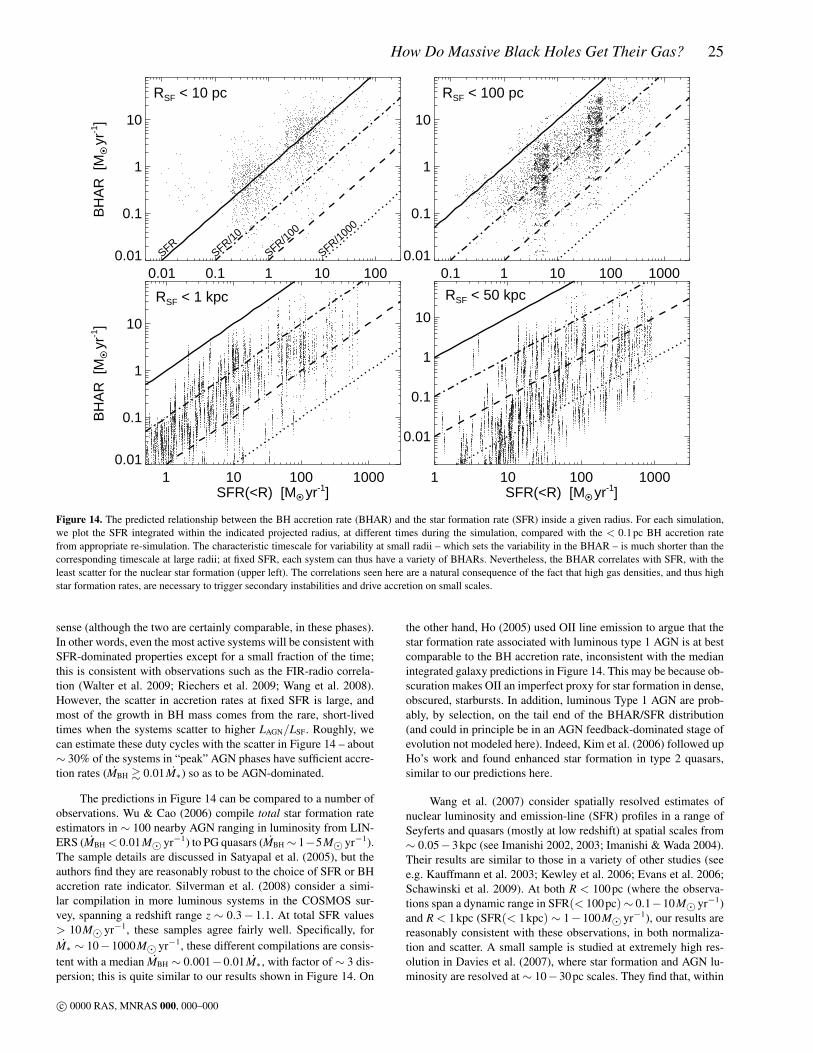
How Do Massive Black Holes Get Their Gas? 25
0.01 0.1 1 10 100
0.01
0.1
1
10
BH
AR
[M
O • y
r-1]
RSF < 10 pc
SFRSFR/10
SFR/100
SFR/1000
0.1 1 10 100 1000
0.01
0.1
1
10
RSF < 100 pc
1 10 100 1000SFR(<R) [M
O • yr-1]
0.01
0.1
1
10
BH
AR
[M
O • y
r-1]
RSF < 1 kpc
1 10 100 1000SFR(<R) [M
O • yr-1]
0.01
0.1
1
10
RSF < 50 kpc
Figure 14. The predicted relationship between the BH accretion rate (BHAR) and the star formation rate (SFR) inside a given radius. For each simulation,we plot the SFR integrated within the indicated projected radius, at different times during the simulation, compared with the < 0.1pc BH accretion ratefrom appropriate re-simulation. The characteristic timescale for variability at small radii – which sets the variability in the BHAR – is much shorter than thecorresponding timescale at large radii; at fixed SFR, each system can thus have a variety of BHARs. Nevertheless, the BHAR correlates with SFR, with theleast scatter for the nuclear star formation (upper left). The correlations seen here are a natural consequence of the fact that high gas densities, and thus highstar formation rates, are necessary to trigger secondary instabilities and drive accretion on small scales.
sense (although the two are certainly comparable, in these phases).In other words, even the most active systems will be consistent withSFR-dominated properties except for a small fraction of the time;this is consistent with observations such as the FIR-radio correla-tion (Walter et al. 2009; Riechers et al. 2009; Wang et al. 2008).However, the scatter in accretion rates at fixed SFR is large, andmost of the growth in BH mass comes from the rare, short-livedtimes when the systems scatter to higher LAGN/LSF. Roughly, wecan estimate these duty cycles with the scatter in Figure 14 – about∼ 30% of the systems in “peak” AGN phases have sufficient accre-tion rates (MBH & 0.01M∗) so as to be AGN-dominated.
The predictions in Figure 14 can be compared to a number ofobservations. Wu & Cao (2006) compile total star formation rateestimators in ∼ 100 nearby AGN ranging in luminosity from LIN-ERS (MBH < 0.01M yr−1) to PG quasars (MBH∼ 1−5M yr−1).The sample details are discussed in Satyapal et al. (2005), but theauthors find they are reasonably robust to the choice of SFR or BHaccretion rate indicator. Silverman et al. (2008) consider a simi-lar compilation in more luminous systems in the COSMOS sur-vey, spanning a redshift range z ∼ 0.3− 1.1. At total SFR values> 10M yr−1, these samples agree fairly well. Specifically, forM∗ ∼ 10−1000M yr−1, these different compilations are consis-tent with a median MBH ∼ 0.001−0.01M∗, with factor of ∼ 3 dis-persion; this is quite similar to our results shown in Figure 14. On
the other hand, Ho (2005) used OII line emission to argue that thestar formation rate associated with luminous type 1 AGN is at bestcomparable to the BH accretion rate, inconsistent with the medianintegrated galaxy predictions in Figure 14. This may be because ob-scuration makes OII an imperfect proxy for star formation in dense,obscured, starbursts. In addition, luminous Type 1 AGN are prob-ably, by selection, on the tail end of the BHAR/SFR distribution(and could in principle be in an AGN feedback-dominated stage ofevolution not modeled here). Indeed, Kim et al. (2006) followed upHo’s work and found enhanced star formation in type 2 quasars,similar to our predictions here.
Wang et al. (2007) consider spatially resolved estimates ofnuclear luminosity and emission-line (SFR) profiles in a range ofSeyferts and quasars (mostly at low redshift) at spatial scales from∼ 0.05−3kpc (see Imanishi 2002, 2003; Imanishi & Wada 2004).Their results are similar to those in a variety of other studies (seee.g. Kauffmann et al. 2003; Kewley et al. 2006; Evans et al. 2006;Schawinski et al. 2009). At both R < 100pc (where the observa-tions span a dynamic range in SFR(< 100pc)∼ 0.1−10M yr−1)and R < 1kpc (SFR(< 1kpc) ∼ 1− 100M yr−1), our results arereasonably consistent with these observations, in both normaliza-tion and scatter. A small sample is studied at extremely high res-olution in Davies et al. (2007), where star formation and AGN lu-minosity are resolved at ∼ 10−30pc scales. They find that, within
c© 0000 RAS, MNRAS 000, 000–000
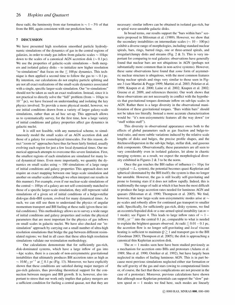
26 Hopkins and Quataert
these radii, the luminosity from star formation is ∼ 1− 5% of thatfrom the BH, again consistent with our prediction here.
7 DISCUSSION
We have presented high resolution smoothed particle hydrody-namic simulations of the dynamics of gas in the central regions ofgalaxies, in order to study gas inflow from galactic scales ∼ 10kpcdown to the scales of a canonical AGN accretion disk (∼ 0.1pc).We use the properties of galactic-scale simulations – both merg-ers and isolated galaxy disks – to initialize new higher resolution“re-simulations” that focus on the . 100 pc dynamics. This tech-nique is then applied a second time to follow the gas to ∼ 0.1 pc.By intention, our calculations do not employ particle splitting andare not all exact realizations of the small-scale dynamics associatedwith a single, specific larger-scale simulation. Our “re-simulations”should not be taken as such an exact realization. Instead, since it isnot practical to directly solve the “full” problem (from ∼ 10kpc to10−5 pc), we have focused on understanding and isolating the keyphysics involved. To provide a more physical model, however, weuse initial conditions drawn from a variety of larger galaxy-scalesimulations, rather than an ad hoc set-up. This approach allowsus to systematically survey, for the first time, how a large varietyof initial conditions and galaxy properties affect gas dynamics ingalactic nuclei.
It is still not feasible, with any numerical scheme, to simul-taneously model the small scales of an AGN accretion disk andthose of a galaxy for cosmological timescales. For this reason, di-rect “zoom-in” approaches have thus far been fairly limited, usuallyevolving each region for just a few local dynamical times. Our nu-merical approach attempts to overcome this severe limitation. First,the smallest regions of each simulation are simulated for many lo-cal dynamical times. Even more importantly, we quantity the dy-namics on small scales using ∼ 100 simulations of a large rangeof initial conditions and galaxy properties This approach does notrequire an exact mapping between one large-scale simulation andanother on smaller scales (although we often interpret our results inthis manner). For example, even if our nuclear-scale simulations ofthe central∼ 100pc of a galaxy are not self-consistently matched tothose of a specific larger-scale simulation, they still represent validsimulations of a given set of initial conditions of a bulge+stellardisk+gas disk+BH system, evolved for many dynamical times. Assuch, we can still use them to understand the physics of angularmomentum transport and BH fueling at these radii (given these ini-tial conditions). This methodology allows us to survey a wide rangeof initial conditions and galaxy properties and isolate the physicalparameters that are most important for the physics of gas inflowson small scales in galactic nuclei. We have also checked our "re-simulation" approach by carrying out a small number of ultra-highresolution simulations that bridge the gap between different resim-ulated regions; we find in all cases that these ultra-high resolutionsimulations validate our resimulation methodology.
Our calculations demonstrate that for sufficiently gas-rich,disk-dominated systems, which have a large inflow of gas into∼kpc scales, there is a cascade of non-axisymmetric gravitationalinstabilities that ultimately produces BH accretion rates as high as∼ 10M yr−1 at . 0.1 pc (Fig. 13). Moreover, we have explicitlyshown that these conditions are satisfied during major mergers ofgas-rich galaxies, thus providing theoretical support for the con-nection between mergers and BH growth. It is, however, also im-portant to stress that our work only implies that galaxy mergers area sufficient condition for fueling a central quasar, not that they are
necessary: similar inflows can be obtained in isolated gas-rich, baror spiral wave-unstable galactic disks.
In broad terms, our results support the “bars within bars” sce-nario proposed in Shlosman et al. (1989). However, we show thatthe secondary instabilities on intermediate scales (∼ 10− 100 pc)exhibit a diverse range of morphologies, including standard nuclearspirals, bars, rings, barred rings, one or three-armed spirals, andirregular/clumpy disks and streams (Fig. 2 & 3). This is very im-portant for comparing to real galaxies: observations have generallyfound that nuclear bars are not ubiquitous in AGN (perhaps notsubstantially more common than in non-active systems). However,these same observations have found that some form of asymmet-ric nuclear structure is ubiquitous, with the most common featuresbeing nuclear spirals and rings very similar to those seen in Fig-ure 3 (see Martini & Pogge 1999; Martini et al. 2003; Peletier et al.1999; Knapen et al. 2000; Laine et al. 2002; Knapen et al. 2002;Greene et al. 2009, and references therein). Our work shows thatthese observations are not necessarily in conflict with the hypothe-sis that gravitational torques dominate inflow on sub-kpc scales inAGN. Rather there is a large diversity in the observational mani-festation of these gravitational torques. “Bars within bars” shouldnot be taken too literally. Instead a more accurate characterizationwould be: “it’s non-axisymmetric features all the way down” (or“stuff within stuff”).
This diversity in observational appearance owes both to theeffects of global parameters such as gas fraction and bulge-to-total ratio, and more subtle variations induced by the relative scalelengths of disks and bulges, the precise profile shapes, and thethickness/dispersion in the sub-kpc bulge, stellar disk, and gaseousdisk components. Observationally, these parameters are all seen tovary considerably even in isolated galaxies, let alone in chaoticmerging systems; as a result, we expect the morphological diver-sity exhibited in Figures 2 & 3 to be the norm.
Once the gas reaches the BH radius of influence (∼ 10pc fora typical ∼ L∗ system), the potential becomes quasi-Keplerian andspherical (dominated by the BH itself); the system is thus no longerbar unstable. However, the gas is still locally self-gravitating andprone to forming stars if it does not inflow rapidly. Indeed, this istraditionally the range of radii at which it has been the most difficultto produce the large accretion rates needed for luminous AGN andquasars (Shlosman et al. 1990; Thompson et al. 2005). We find,however, that new large-scale non-axisymmetric modes arise at ∼pc-scales and robustly allow for continued gas transport to smallerradii. Specifically, for sufficiently gas-rich, disky systems, we findan eccentric/lopsided disk or a one-armed spiral instability (an m =1 mode); see Figure 4. This leads to large inflow rates of ∼ 1−10M yr−1 into the central 0.1 pc, comparable to what is neededto explain the brightest quasars observed. At radii . 0.01−0.1 pc,the accretion flow is no longer self-gravitating and local viscousheating is sufficient to maintain Q & 1 and transport gas to the BH(Goodman 2003; Thompson et al. 2005); the disk is approaching acanonical thin Keplerian accretion disk.
The m = 1 modes seen here have been studied previously asa mechanism for accretion onto BHs and protostars (Adams et al.1989; Shu et al. 1990; Ostriker et al. 1992), but have largely beenneglected in studies of fueling luminous AGN. This is in part be-cause most previous simulations neglected either star formation orthe self-gravity of the gas and stars (owing to computational limitsor, of course, the fact that these complications are not present in thecase of a protostar). Moreover, previous calculations have shownthat although near-Keplerian potentials can support the “slow” pat-tern speed m = 1 modes we find here, such modes are linearly
c© 0000 RAS, MNRAS 000, 000–000
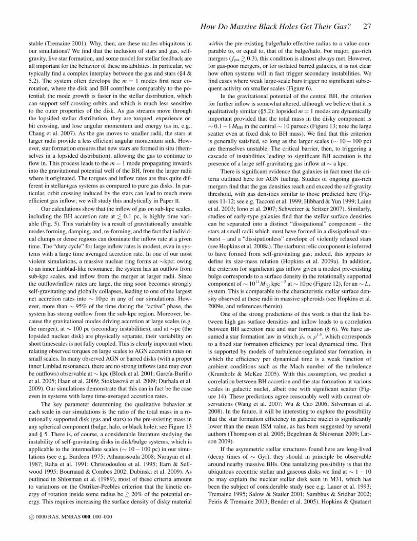
How Do Massive Black Holes Get Their Gas? 27
stable (Tremaine 2001). Why, then, are these modes ubiquitous inour simulations? We find that the inclusion of stars and gas, self-gravity, live star formation, and some model for stellar feedback areall important for the behavior of these instabilities. In particular, wetypically find a complex interplay between the gas and stars (§4 &5.2). The system often develops the m = 1 modes first near co-rotation, where the disk and BH contribute comparably to the po-tential; the mode growth is faster in the stellar distribution, whichcan support self-crossing orbits and which is much less sensitiveto the outer properties of the disk. As gas streams move throughthe lopsided stellar distribution, they are torqued, experience or-bit crossing, and lose angular momentum and energy (as in, e.g.,Chang et al. 2007). As the gas moves to smaller radii, the stars atlarger radii provide a less efficient angular momentum sink. How-ever, star formation ensures that new stars are formed in situ (them-selves in a lopsided distribution), allowing the gas to continue toflow in. This process leads to the m = 1 mode propagating inwardsinto the gravitational potential well of the BH, from the larger radiiwhere it originated. The torques and inflow rates are thus quite dif-ferent in stellar+gas systems as compared to pure gas disks. In par-ticular, orbit crossing induced by the stars can lead to much moreefficient gas inflow; we will study this analytically in Paper II.
Our calculations show that the inflow of gas on sub-kpc scales,including the BH accretion rate at . 0.1 pc, is highly time vari-able (Fig. 5). This variability is a result of gravitationally unstablemodes forming, damping, and, re-forming, and the fact that individ-ual clumps or dense regions can dominate the inflow rate at a giventime. The “duty cycle” for large inflow rates is modest, even in sys-tems with a large time averaged accretion rate. In one of our mostviolent simulations, a massive nuclear ring forms at ∼kpc; owingto an inner Linblad-like resonance, the system has an outflow fromsub-kpc scales, and inflow from the merger at larger radii. Sincethe outflow/inflow rates are large, the ring soon becomes stronglyself-gravitating and globally collapses, leading to one of the largestnet accretion rates into ∼ 10pc in any of our simulations. How-ever, more than ∼ 95% of the time during the “active” phase, thesystem has strong outflow from the sub-kpc region. Moreover, be-cause the gravitational modes driving accretion at large scales (e.g.the merger), at ∼ 100 pc (secondary instabilities), and at ∼pc (thelopsided nuclear disk) are physically separate, their variability onshort timescales is not fully coupled. This is clearly important whenrelating observed torques on large scales to AGN accretion rates onsmall scales. In many observed AGN or barred disks (with a properinner Linblad resonance), there are no strong inflows (and may evenbe outflows) observable at∼ kpc (Block et al. 2001; García-Burilloet al. 2005; Haan et al. 2009; Stoklasová et al. 2009; Durbala et al.2009). Our simulations demonstrate that this can in fact be the caseeven in systems with large time-averaged accretion rates.
The key parameter determining the qualitative behavior ateach scale in our simulations is the ratio of the total mass in a ro-tationally supported disk (gas and stars) to the pre-existing mass inany spherical component (bulge, halo, or black hole); see Figure 13and § 5. There is, of course, a considerable literature studying theinstability of self-gravitating disks in disk/bulge systems, which isapplicable to the intermediate scales (∼ 10− 100 pc) in our simu-lations (see e.g. Bardeen 1975; Athanassoula 2008; Narayan et al.1987; Raha et al. 1991; Christodoulou et al. 1995; Earn & Sell-wood 1995; Bournaud & Combes 2002; Dubinski et al. 2009). Asoutlined in Shlosman et al. (1989), most of these criteria amountto variations on the Ostriker-Peebles criterion that the kinetic en-ergy of rotation inside some radius be & 20% of the potential en-ergy. This requires increasing the surface density of disky material
within the pre-existing bulge/halo effective radius to a value com-parable to, or equal to, that of the bulge/halo. For major, gas-richmergers ( fgas & 0.3), this condition is almost always met. However,for gas-poor mergers, or for isolated barred galaxies, it is not clearhow often systems will in fact trigger secondary instabilities. Wefind cases where weak large-scale bars trigger no significant subse-quent activity on smaller scales (Figure 6).
In the gravitational potential of the central BH, the criterionfor further inflow is somewhat altered, although we believe that it isqualitatively similar (§5.2): lopsided m = 1 modes are dynamicallyimportant provided that the total mass in the disky component is∼ 0.1−1MBH in the central∼ 10 parsecs (Figure 13; note the largescatter even at fixed disk to BH mass). We find that this criterionis generally satisfied, so long as the larger scales (∼ 10− 100 pc)are themselves unstable. The critical barrier, then, to triggering acascade of instabilities leading to significant BH accretion is thepresence of a large self-gravitating gas inflow at ∼ a kpc.
There is significant evidence that galaxies in fact meet the cri-teria outlined here for AGN fueling. Studies of ongoing gas-richmergers find that the gas densities reach and exceed the self-gravitythreshold, with gas densities similar to those predicted here (Fig-ures 11-12; see e.g. Tacconi et al. 1999; Hibbard & Yun 1999; Laineet al. 2003; Iono et al. 2007; Schweizer & Seitzer 2007). Similarly,studies of early-type galaxies find that the stellar surface densitiescan be separated into a distinct “dissipational” component – thestars at small radii which must have formed in a dissipational star-burst – and a “dissipationless” envelope of violently relaxed stars(see Hopkins et al. 2008a). The starburst relic component is inferredto have formed from self-gravitating gas; indeed, this appears todefine its size-mass relation (Hopkins et al. 2009a). In addition,the criterion for significant gas inflow given a modest pre-existingbulge corresponds to a surface density in the rotationally supportedcomponent of∼ 1011 M kpc−2 at∼ 10pc (Figure 12), for an∼ L∗system. This is comparable to the characteristic stellar surface den-sity observed at these radii in massive spheroids (see Hopkins et al.2009e, and references therein).
One of the strong predictions of this work is that the link be-tween high gas surface densities and inflow leads to a correlationbetween BH accretion rate and star formation (§ 6). We have as-sumed a star formation law in which ρ∗ ∝ ρ1.5, which correspondsto a fixed star formation efficiency per local dynamical time. Thisis supported by models of turbulence-regulated star formation, inwhich the efficiency per dynamical time is a weak function ofambient conditions such as the Mach number of the turbulence(Krumholz & McKee 2005). With this assumption, we predict acorrelation between BH accretion and the star formation at variousscales in galactic nuclei, albeit one with significant scatter (Fig-ure 14). These predictions agree reasonably well with current ob-servations (Wang et al. 2007; Wu & Cao 2006; Silverman et al.2008). In the future, it will be interesting to explore the possibilitythat the star formation efficiency in galactic nuclei is significantlylower than the mean ISM value, as has been suggested by severalauthors (Thompson et al. 2005; Begelman & Shlosman 2009; Lar-son 2009).
If the asymmetric stellar structures found here are long-lived(decay times of ∼ Gyr), they should in principle be observablearound nearby massive BHs. One tantalizing possibility is that theubiquitous eccentric stellar and gaseous disks we find at ∼ 1− 10pc may explain the nuclear stellar disk seen in M31, which hasbeen the subject of considerable study (see e.g. Lauer et al. 1993;Tremaine 1995; Salow & Statler 2001; Sambhus & Sridhar 2002;Peiris & Tremaine 2003; Bender et al. 2005). Hopkins & Quataert
c© 0000 RAS, MNRAS 000, 000–000
28 Hopkins and Quataert
(2010) examine this possibility in detail and show that the spa-tial scales ∼ 1− 10pc, moderate eccentricities, and stellar masses∼ 0.1−1MBH found in our simulations are all comparable to thoseobserved. Eccentric nuclear disks have also been observed (albeitin less detail) around a number of other massive but inactive BHs,including NGC4486b (Lauer et al. 1996), M83 (Thatte et al. 2000),and VCC128 (Debattista et al. 2006). This strongly suggests thatwe can probe the the instabilities that produced the growth of mas-sive BHs in the “fossil” relics of that accretion.
The dominant uncertainties in the models presented here areour treatment of the ISM physics, star formation, and feedback.Lacking a full micro-physical understanding of these processes – orthe resolution to directly incorporate such a model – it is necessaryto adopt a sub-resolution prescription for their impact. Our modelis that stars form at all radii, in local, self-gravitating clumps, witha fixed efficiency relative to the local dynamical time. In addition,feedback from stars (supernovae, radiation, stellar winds/outflows,etc.) contributes, potentially along with cosmic rays and magneticfields, to generating a turbulent velocity that is much larger than thethermal sound speed of the ISM. It is this turbulent “sound speed”that is included in our ISM equation of state (Figure 1). Observa-tions suggest that these assumptions are at least plausible even atthe small scales we model here: a local Kennicutt-Schmidt relationholds in nuclear starbursts and on small scales in galaxies (Kenni-cutt 1998; Kennicutt et al. 2007; Bigiel et al. 2008) and star forma-tion efficiencies per dynamical time do not appear to evolve even invery dense regions (comparable to the highest gas densities mod-eled here; see, e.g., Tan et al. 2006; Krumholz & Tan 2007). More-over, AGN are observed to have associated nuclear star formationon scales as small as a pc; the densities of stars formed in situ atthese scales (Davies et al. 2007; Hicks et al. 2009) are reasonablyconsistent with our predictions. Large turbulent and/or non-thermalgas velocity dispersions are also ubiquitous, from starburst nucleion ∼kpc scales to the sub-pc scales around AGN probed by watermasers (Downes & Solomon 1998; Westmoquette et al. 2007; Tac-coni et al. 1999; Iono et al. 2007; Kondratko et al. 2005); these ob-servations motivate our choice of sub-resolution feedback models(Figure 1). To study the impact of ISM uncertainties on our results,we explicitly used different star formation efficiencies in some ofour simulations; although this does have a quantitative affect on theresulting gas densities and inflow rates, the physical processes thatwe have identified as driving accretion remain the same.
As noted in §2, the primary consequence of the large effectivesound speed in our models is to increase the Jeans and Toomremasses, thus suppressing the formation of small-scale structure.That is, we effectively smooth over the smaller scales on whichour treatment of the ISM physics is not appropriate. This impliesthat in our model, most of the gas, most of the time, resides in rel-atively diffuse structures, rather than being bound to very compactclusters, as would be the case if we did not include stellar feed-back and/or a sub-grid sound speed (see Appendix B). We suspectthat this approach is reasonable for the global gravitational dynam-ics highlighted in this paper. In particular, our calculations indicatethat over a remarkably large dynamic range, from 0.1pc to 10kpc,the torques and angular momentum transport are gravitational, andscale simply with the magnitude of the asymmetry in the potential,not with the sound speed of the gas (Fig. 9 and §4). In Paper II, wewill present a more detailed comparison between analytic modelsand our numerical results that supports this conclusion.
In our calculations, we have neglected AGN feedback in orderto study how gas gets down to a BH in the first place. To the ex-tent that feedback is important on these scales, our simulations may
better approximate the “early” stages of BH growth, when the BHis still relatively small (compared to, e.g., the still-forming bulge),and before it reaches a critical mass or luminosity at which feed-back becomes dynamically important. When BH growth becomesself-regulated, inflow and outflow are coupled, and the problem ofAGN fueling must be addressed with a model that includes AGNfeedback as a function of gas properties and spatial scale.
ACKNOWLEDGMENTS
We thank Phil Chang, Lars Hernquist, Norm Murray, andVolker Springel for helpful discussions during the development ofthis work, and the referee for a careful reading of the text and anumber of very useful suggestions. PFH and EQ were supportedby the Miller Institute for Basic Research in Science, Universityof California Berkeley. EQ was also supported in part by NASAgrant NNG06GI68G and the David and Lucile Packard Foundation.
REFERENCES
Adams, F. C., Ruden, S. P., & Shu, F. H. 1989, ApJ, 347, 959Allen, L., et al. 2007, in Protostars and Planets V, ed. B. Reipurth,
D. Jewitt, & K. Keil, 361–376Aller, M. C., & Richstone, D. O. 2007, ApJ, 665, 120Aoki, S., Noguchi, M., & Iye, M. 1979, PASJ, 31, 737Athanassoula, E. 2008, MNRAS, 390, L69Athanassoula, E., Bienayme, O., Martinet, L., & Pfenniger, D.
1983, A&A, 127, 349Athanassoula, E., Lambert, J. C., & Dehnen, W. 2005, MNRAS,
363, 496Balbus, S. A., & Hawley, J. F. 1998, Reviews of Modern Physics,
70, 1Banerjee, R., Pudritz, R. E., & Holmes, L. 2004, MNRAS, 355,
248Bardeen, J. M. 1975, in IAU Symposium, Vol. 69, Dynamics of
the Solar Systems, ed. A. Hayli, 297–+Barnes, J. E. 1998, in Saas-Fee Advanced Course 26: Galax-
ies: Interactions and Induced Star Formation; Springer-VerlagBerlin/Heidelberg, ed. R. C. Kennicutt, Jr., F. Schweizer, J. E.Barnes, D. Friedli, L. Martinet, & D. Pfenniger, 275–+
Barnes, J. E., & Hernquist, L. 1996, ApJ, 471, 115Barnes, J. E., & Hernquist, L. E. 1991, ApJL, 370, L65Begelman, M., & Shlosman, I. 2009, ApJL, in press,
arXiv:0904.4247, 0904, 4247Bell, E. F., & de Jong, R. S. 2001, ApJ, 550, 212Bender, R., et al. 2005, ApJ, 631, 280Berentzen, I., Shlosman, I., Martinez-Valpuesta, I., & Heller,
C. H. 2007, ApJ, 666, 189Bigiel, F., Leroy, A., Walter, F., Brinks, E., de Blok, W. J. G.,
Madore, B., & Thornley, M. D. 2008, AJ, 136, 2846Blitz, L. 1993, in Protostars and Planets III (University of Arizona
Press: Tucson), ed. E. H. Levy & J. I. Lunine, 125–161Block, D. L., Puerari, I., Knapen, J. H., Elmegreen, B. G., Buta,
R., Stedman, S., & Elmegreen, D. M. 2001, Astronomy and As-trophysics, 375, 761
Böker, T., Sarzi, M., McLaughlin, D. E., van der Marel, R. P., Rix,H.-W., Ho, L. C., & Shields, J. C. 2004, AJ, 127, 105
Boley, A. C., Mejía, A. C., Durisen, R. H., Cai, K., Pickett, M. K.,& D’Alessio, P. 2006, ApJ, 651, 517
Bonnell, I. A., Dobbs, C. L., Robitaille, T. P., & Pringle, J. E.2006, MNRAS, 365, 37
c© 0000 RAS, MNRAS 000, 000–000
How Do Massive Black Holes Get Their Gas? 29
Bouché, N., et al. 2007, ApJ, 671, 303Bournaud, F., & Combes, F. 2002, A&A, 392, 83Bournaud, F., Combes, F., Jog, C. J., & Puerari, I. 2005, A&A,
438, 507Bryant, P. M., & Scoville, N. Z. 1999, AJ, 117, 2632Bullock, J. S., et al. 2001, MNRAS, 321, 559Cai, K., Durisen, R. H., Boley, A. C., Pickett, M. K., & Mejía,
A. C. 2008, ApJ, 673, 1138Carlberg, R. G. 1986, ApJ, 310, 593Chang, P., Murray-Clay, R., Chiang, E., & Quataert, E. 2007, The
Astrophysical Journal, 668, 236Christodoulou, D. M., Shlosman, I., & Tohline, J. E. 1995, ApJ,
443, 551Cossins, P., Lodato, G., & Clarke, C. J. 2009, MNRAS, 393, 1157Côté, P., et al. 2006, ApJS, 165, 57Covington, M., Dekel, A., Cox, T. J., Jonsson, P., & Primack, J. R.
2008, MNRAS, 384, 94Cox, T. J., Dutta, S. N., Di Matteo, T., Hernquist, L., Hopkins,
P. F., Robertson, B., & Springel, V. 2006, ApJ, 650, 791Cuadra, J., Armitage, P. J., Alexander, R. D., & Begelman, M. C.
2009, Monthly Notices of the Royal Astronomical Society, 393,1423
Dasyra, K. M., et al. 2006, ApJ, 638, 745—. 2007, ApJ, 657, 102Davies, R. I., Sánchez, F. M., Genzel, R., Tacconi, L. J., Hicks,
E. K. S., Friedrich, S., & Sternberg, A. 2007, ApJ, 671, 1388Debattista, V. P., Ferreras, I., Pasquali, A., Seth, A., De Rijcke, S.,
& Morelli, L. 2006, ApJL, 651, L97DeBuhr, J., Quataert, E., Ma, C.-P., & Hopkins, P. 2009, MNRAS,
in press, arXiv:0909.2872Di Matteo, T., Springel, V., & Hernquist, L. 2005, Nature, 433,
604Dotti, M., Ruszkowski, M., Paredi, L., Colpi, M., Volonteri, M.,
& Haardt, F. 2009, MNRAS, 396, 1640Downes, D., & Solomon, P. M. 1998, ApJ, 507, 615Dubinski, J., Berentzen, I., & Shlosman, I. 2009, ApJ, 697, 293Durbala, A., Buta, R., Sulentic, J. W., & Verdes-Montenegro, L.
2009, MNRAS, in press [arXiv:0905.2340]Earn, D. J. D., & Sellwood, J. A. 1995, ApJ, 451, 533Elmegreen, B. G. 2007, ApJ, 668, 1064Escala, A. 2007, ApJ, 671, 1264Escala, A., Larson, R. B., Coppi, P. S., & Mardones, D. 2004, ApJ,
607, 765Evans, A. S., Solomon, P. M., Tacconi, L. J., Vavilkin, T., &
Downes, D. 2006, AJ, 132, 2398Ferrarese, L., & Merritt, D. 2000, ApJL, 539, L9Ferrarese, L., et al. 2006a, ApJL, 644, L21—. 2006b, ApJS, 164, 334Förster Schreiber, N. M., et al. 2006, ApJ, 645, 1062Gammie, C. F. 2001, ApJ, 553, 174García-Burillo, S., Combes, F., Schinnerer, E., Boone, F., & Hunt,
L. K. 2005, Astronomy and Astrophysics, 441, 1011Gebhardt, K., et al. 2000, ApJL, 539, L13Goodman, J. 2003, MNRAS, 339, 937Greene, J. E., Zakamska, N. L., Liu, X., Barth, A. J., & Ho, L. C.
2009, ApJ, in press, arXiv:0907.1086Gunn, J. E. 1987, in Nearly Normal Galaxies. From the Planck
Time to the Present (New York: Springer-Verlag), ed. S. M.Faber, 455–464
Haan, S., Schinnerer, E., Emsellem, E., García-Burillo, S.,Combes, F., Mundell, C. G., & Rix, H.-W. 2009, The Astrophys-ical Journal, 692, 1623
Heller, C., Shlosman, I., & Englmaier, P. 2001, The AstrophysicalJournal, 553, 661
Hernquist, L. 1989, Nature, 340, 687—. 1990, ApJ, 356, 359—. 1993, ApJ, 404, 717Hernquist, L., & Ostriker, J. P. 1992, Astrophysical Journal, 386,
375Hernquist, L., Spergel, D. N., & Heyl, J. S. 1993, ApJ, 416, 415Hibbard, J. E., & Yun, M. S. 1999, ApJL, 522, L93Hicks, E. K. S., Davies, R. I., Malkan, M. A., Genzel, R., Tacconi,
L. J., Sánchez, F. M., & Sternberg, A. 2009, ApJ, 696, 448Ho, L. C. 2005, ApJ, 629, 680Hopkins, P. F., Cox, T. J., Dutta, S. N., Hernquist, L., Kormendy,
J., & Lauer, T. R. 2009a, ApJS, 181, 135Hopkins, P. F., Cox, T. J., & Hernquist, L. 2008a, ApJ, 689, 17Hopkins, P. F., Cox, T. J., Younger, J. D., & Hernquist, L. 2009b,
ApJ, 691, 1168Hopkins, P. F., & Hernquist, L. 2006, ApJS, 166, 1—. 2009, MNRAS, in press, arXiv:0910.4582Hopkins, P. F., Hernquist, L., Cox, T. J., Dutta, S. N., & Rothberg,
B. 2008b, ApJ, 679, 156Hopkins, P. F., Hernquist, L., Cox, T. J., Kereš, D., & Wuyts, S.
2009c, ApJ, 691, 1424Hopkins, P. F., Hernquist, L., Cox, T. J., Robertson, B., & Krause,
E. 2007, ApJ, 669, 67Hopkins, P. F., Hernquist, L., Martini, P., Cox, T. J., Robertson,
B., Di Matteo, T., & Springel, V. 2005, ApJL, 625, L71Hopkins, P. F., Lauer, T. R., Cox, T. J., Hernquist, L., & Kor-
mendy, J. 2009d, ApJS, 181, 486Hopkins, P. F., Murray, N., Quataert, E., & Thompson, T. A.
2009e, MNRAS, in press, arXiv:0908.4088Hopkins, P. F., & Quataert, E. 2010, MNRAS, L62+Hopkins, P. F., Somerville, R. S., Cox, T. J., Hernquist, L., Jogee,
S., Kereš, D., Ma, C.-P., Robertson, B., & Stewart, K. 2009f,MNRAS, 397, 802
Imanishi, M. 2002, ApJ, 569, 44—. 2003, ApJ, 599, 918Imanishi, M., & Wada, K. 2004, ApJ, 617, 214Iono, D., et al. 2007, ApJ, 659, 283Jogee, S. 2006, in Lecture Notes in Physics, Berlin Springer Ver-
lag, Vol. 693, Physics of Active Galactic Nuclei at all Scales, ed.D. Alloin, 143–+
Jogee, S., Scoville, N., & Kenney, J. D. P. 2005, ApJ, 630, 837Johansson, P. H., Naab, T., & Burkert, A. 2009a, ApJ, 690, 802—. 2009b, ApJL, in press, arXiv:0910.2232Kalnajs, A. J. 1971, ApJ, 166, 275Kauffmann, G., et al. 2003, MNRAS, 346, 1055Kawakatu, N., & Wada, K. 2008, ApJ, 681, 73Kennicutt, Jr., R. C. 1998, ApJ, 498, 541Kennicutt, Jr., R. C., et al. 2007, ApJ, 671, 333Kewley, L. J., Groves, B., Kauffmann, G., & Heckman, T. 2006,
MNRAS, 372, 961Kim, M., Ho, L. C., & Im, M. 2006, ApJ, 642, 702Knapen, J. H., Pérez-Ramírez, D., & Laine, S. 2002, Monthly No-
tice of the Royal Astronomical Society, 337, 808Knapen, J. H., Shlosman, I., & Peletier, R. F. 2000, ApJ, 529, 93Kondratko, P. T., Greenhill, L. J., & Moran, J. M. 2005, ApJ, 618,
618Kormendy, J. 1989, ApJL, 342, L63Kormendy, J., Fisher, D. B., Cornell, M. E., & Bender, R. 2009,
ApJS, 182, 216Kormendy, J., & Freeman, K. C. 2004, in IAU Symposium,
c© 0000 RAS, MNRAS 000, 000–000

30 Hopkins and Quataert
Vol. 220, Dark Matter in Galaxies, ed. S. Ryder, D. Pisano,M. Walker, & K. Freeman, 377–+
Kormendy, J., & Richstone, D. 1995, ARA&A, 33, 581Krips, M., et al. 2007, A&A, 468, L63Krumholz, M. R., Klein, R. I., & McKee, C. F. 2007, ApJ, 656,
959Krumholz, M. R., Matzner, C. D., & McKee, C. F. 2006, ApJ,
653, 361Krumholz, M. R., & McKee, C. F. 2005, ApJ, 630, 250Krumholz, M. R., & Tan, J. C. 2007, ApJ, 654, 304Laine, S., Shlosman, I., Knapen, J. H., & Peletier, R. F. 2002, The
Astrophysical Journal, 567, 97Laine, S., van der Marel, R. P., Rossa, J., Hibbard, J. E., Mihos,
J. C., Böker, T., & Zabludoff, A. I. 2003, AJ, 126, 2717Larson, R. B. 1981, MNRAS, 194, 809—. 2009, Nature, in press, arXiv:0909.3110Lau, Y. Y., & Bertin, G. 1978, ApJ, 226, 508Lauer, T. R., et al. 1993, AJ, 106, 1436—. 1996, ApJL, 471, L79+—. 2007, ApJ, 664, 226Lemoine-Busserolle, M., Bunker, A., Lamareille, F., & Kissler-
Patig, M. 2009, MNRAS, in press, arXiv:0909.1386Levine, R., Gnedin, N. Y., Hamilton, A. J. S., & Kravtsov, A. V.
2008, ApJ, 678, 154Lodato, G., & Rice, W. K. M. 2004, MNRAS, 351, 630Lynden-Bell, D., & Kalnajs, A. J. 1972, MNRAS, 157, 1Magorrian, J., et al. 1998, AJ, 115, 2285Mandelbaum, R., Seljak, U., Kauffmann, G., Hirata, C. M., &
Brinkmann, J. 2006, MNRAS, 368, 715Martini, P. 2004, in Coevolution of Black Holes and Galaxies
(Cambridge: Cambridge University Press), ed. L. C. Ho, 169Martini, P., & Pogge, R. W. 1999, Astron. J., 118, 2646Martini, P., Regan, M. W., Mulchaey, J. S., & Pogge, R. W. 2003,
ApJ, 589, 774Mayer, L., Kazantzidis, S., Madau, P., Colpi, M., Quinn, T., &
Wadsley, J. 2007, Science, 316, 1874McKee, C. F., & Ostriker, J. P. 1977, ApJ, 218, 148Mihos, J. C., & Hernquist, L. 1994, ApJL, 431, L9—. 1996, ApJ, 464, 641Murray, N., Quataert, E., & Thompson, T. A. 2009, ApJ, in press
[arXiv:0906.5358]Narayan, R., Goldreich, P., & Goodman, J. 1987, MNRAS, 228, 1Nayakshin, S., Cuadra, J., & Springel, V. 2007, MNRAS, 379, 21Nayakshin, S., & King, A. 2007, MNRAS, in press,
arXiv:0705.1686Noguchi, M. 1988, A&A, 203, 259O’Shea, B. W., Nagamine, K., Springel, V., Hernquist, L., & Nor-
man, M. L. 2005, ApJS, 160, 1Ostriker, E. C., Shu, F. H., & Adams, F. C. 1992, ApJ, 399, 192Ostriker, J. P. 1980, Comments on Astrophysics, 8, 177Peiris, H. V., & Tremaine, S. 2003, ApJ, 599, 237Peletier, R. F., et al. 1999, ApJS, 125, 363Perets, H. B., & Alexander, T. 2008, ApJ, 677, 146Perets, H. B., Hopman, C., & Alexander, T. 2007, ApJ, 656, 709Quillen, A. C., Frogel, J. A., Kenney, J. D. P., Pogge, R. W., &
Depoy, D. L. 1995, ApJ, 441, 549Raha, N., Sellwood, J. A., James, R. A., & Kahn, F. D. 1991,
Nature, 352, 411Rice, W. K. M., Lodato, G., & Armitage, P. J. 2005, MNRAS,
364, L56Riechers, D. A., Walter, F., Bertoldi, F., Carilli, C. L., Aravena,
M., Neri, R., Cox, P., Weiss, A., & Menten, K. M. 2009, ApJ, inpress, arXiv:0908.0018
Robertson, B., Bullock, J. S., Cox, T. J., Di Matteo, T., Hernquist,L., Springel, V., & Yoshida, N. 2006a, ApJ, 645, 986
Robertson, B., Hernquist, L., Cox, T. J., Di Matteo, T., Hopkins,P. F., Martini, P., & Springel, V. 2006b, ApJ, 641, 90
Sakamoto, K., Okumura, S. K., Ishizuki, S., & Scoville, N. Z.1999, The Astrophysical Journal, 525, 691
Salow, R. M., & Statler, T. S. 2001, ApJL, 551, L49Salucci, P., Szuszkiewicz, E., Monaco, P., & Danese, L. 1999,
MNRAS, 307, 637Sambhus, N., & Sridhar, S. 2002, A&A, 388, 766Sanders, D. B., & Mirabel, I. F. 1996, ARA&A, 34, 749Sanders, D. B., Soifer, B. T., Elias, J. H., Madore, B. F., Matthews,
K., Neugebauer, G., & Scoville, N. Z. 1988a, ApJ, 325, 74Sanders, D. B., Soifer, B. T., Elias, J. H., Neugebauer, G., &
Matthews, K. 1988b, ApJL, 328, L35Satyapal, S., Dudik, R. P., O’Halloran, B., & Gliozzi, M. 2005,
ApJ, 633, 86Schartmann, M., Meisenheimer, K., Klahr, H., Camenzind, M.,
Wolf, S., & Henning, T. 2009, MNRAS, 393, 759Schawinski, K., et al. 2009, eprint arXiv, 0903, 3415Schweizer, F. 1998, in Saas-Fee Advanced Course 26: Galax-
ies: Interactions and Induced Star Formation (Springer-VerlagBerlin/Heidelberg), ed. R. C. Kennicutt, Jr., F. Schweizer, J. E.Barnes, D. Friedli, L. Martinet, & D. Pfenniger, 105–+
Schweizer, F., & Seitzer, P. 2007, AJ, 133, 2132Shankar, F., Salucci, P., Granato, G. L., De Zotti, G., & Danese,
L. 2004, MNRAS, 354, 1020Shlosman, I., & Begelman, M. C. 1989, ApJ, 341, 685Shlosman, I., Begelman, M. C., & Frank, J. 1990, Nature, 345,
679Shlosman, I., Frank, J., & Begelman, M. C. 1989, Nature, 338, 45Shu, F. H., Tremaine, S., Adams, F. C., & Ruden, S. P. 1990, ApJ,
358, 495Silverman, J. D., et al. 2008, eprint arXiv, 0810, 3653Soltan, A. 1982, MNRAS, 200, 115Springel, V. 2005, MNRAS, 364, 1105Springel, V., Di Matteo, T., & Hernquist, L. 2005a, ApJL, 620,
L79—. 2005b, MNRAS, 361, 776Springel, V., & Hernquist, L. 2002, MNRAS, 333, 649—. 2003, MNRAS, 339, 289—. 2005, ApJL, 622, L9Stoklasová, I., Ferruit, P., Emsellem, E., Jungwiert, B., Pécontal,
E., & Sánchez, S. F. 2009, A&A, in press [arXiv:0905.3349]Tacconi, L. J., Genzel, R., Tecza, M., Gallimore, J. F., Downes,
D., & Scoville, N. Z. 1999, ApJ, 524, 732Tacconi, L. J., et al. 2006, ApJ, 640, 228Tan, J. C., Krumholz, M. R., & McKee, C. F. 2006, ApJL, 641,
L121Thatte, N., Tecza, M., & Genzel, R. 2000, A&A, 364, L47Thompson, T. A., Quataert, E., & Murray, N. 2005, ApJ, 630, 167Toomre, A. 1977, ARA&A, 15, 437Tremaine, S. 1995, AJ, 110, 628—. 2001, AJ, 121, 1776Veilleux, S., et al. 2009, ApJ, 701, 587Vorobyov, E. I., & Basu, S. 2006, ApJ, 650, 956—. 2009, MNRAS, 393, 822Wada, K., & Norman, C. A. 2002, ApJL, 566, L21Wada, K., Papadopoulos, P., & Spaans, M. 2009, ApJ, in press,
arXiv:0906.5444
c© 0000 RAS, MNRAS 000, 000–000
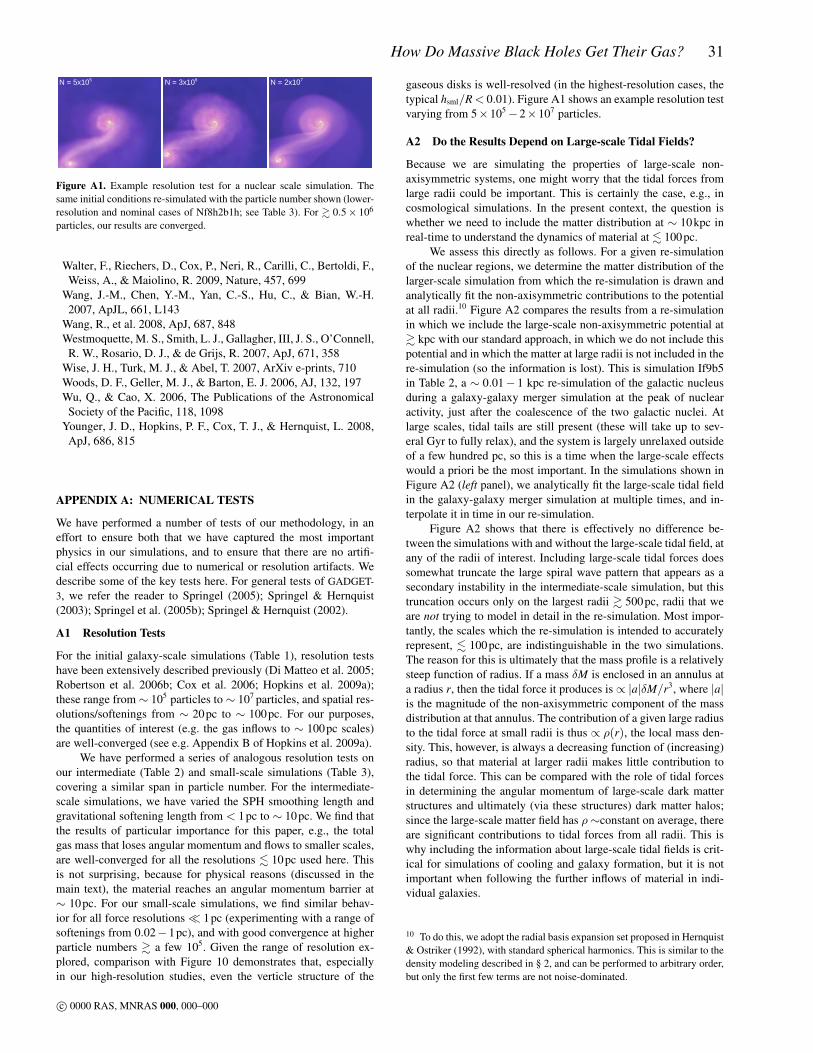
How Do Massive Black Holes Get Their Gas? 31
N = 5x10⁵ N = 3x10⁶ N = 2x10⁷
Figure A1. Example resolution test for a nuclear scale simulation. Thesame initial conditions re-simulated with the particle number shown (lower-resolution and nominal cases of Nf8h2b1h; see Table 3). For & 0.5× 10⁶
particles, our results are converged.
Walter, F., Riechers, D., Cox, P., Neri, R., Carilli, C., Bertoldi, F.,Weiss, A., & Maiolino, R. 2009, Nature, 457, 699
Wang, J.-M., Chen, Y.-M., Yan, C.-S., Hu, C., & Bian, W.-H.2007, ApJL, 661, L143
Wang, R., et al. 2008, ApJ, 687, 848Westmoquette, M. S., Smith, L. J., Gallagher, III, J. S., O’Connell,
R. W., Rosario, D. J., & de Grijs, R. 2007, ApJ, 671, 358Wise, J. H., Turk, M. J., & Abel, T. 2007, ArXiv e-prints, 710Woods, D. F., Geller, M. J., & Barton, E. J. 2006, AJ, 132, 197Wu, Q., & Cao, X. 2006, The Publications of the Astronomical
Society of the Pacific, 118, 1098Younger, J. D., Hopkins, P. F., Cox, T. J., & Hernquist, L. 2008,
ApJ, 686, 815
APPENDIX A: NUMERICAL TESTS
We have performed a number of tests of our methodology, in aneffort to ensure both that we have captured the most importantphysics in our simulations, and to ensure that there are no artifi-cial effects occurring due to numerical or resolution artifacts. Wedescribe some of the key tests here. For general tests of GADGET-3, we refer the reader to Springel (2005); Springel & Hernquist(2003); Springel et al. (2005b); Springel & Hernquist (2002).
A1 Resolution Tests
For the initial galaxy-scale simulations (Table 1), resolution testshave been extensively described previously (Di Matteo et al. 2005;Robertson et al. 2006b; Cox et al. 2006; Hopkins et al. 2009a);these range from ∼ 105 particles to ∼ 107 particles, and spatial res-olutions/softenings from ∼ 20pc to ∼ 100pc. For our purposes,the quantities of interest (e.g. the gas inflows to ∼ 100pc scales)are well-converged (see e.g. Appendix B of Hopkins et al. 2009a).
We have performed a series of analogous resolution tests onour intermediate (Table 2) and small-scale simulations (Table 3),covering a similar span in particle number. For the intermediate-scale simulations, we have varied the SPH smoothing length andgravitational softening length from < 1pc to ∼ 10pc. We find thatthe results of particular importance for this paper, e.g., the totalgas mass that loses angular momentum and flows to smaller scales,are well-converged for all the resolutions . 10pc used here. Thisis not surprising, because for physical reasons (discussed in themain text), the material reaches an angular momentum barrier at∼ 10pc. For our small-scale simulations, we find similar behav-ior for all force resolutions 1pc (experimenting with a range ofsoftenings from 0.02−1pc), and with good convergence at higherparticle numbers & a few 105. Given the range of resolution ex-plored, comparison with Figure 10 demonstrates that, especiallyin our high-resolution studies, even the verticle structure of the
gaseous disks is well-resolved (in the highest-resolution cases, thetypical hsml/R< 0.01). Figure A1 shows an example resolution testvarying from 5×10⁵−2×10⁷ particles.
A2 Do the Results Depend on Large-scale Tidal Fields?
Because we are simulating the properties of large-scale non-axisymmetric systems, one might worry that the tidal forces fromlarge radii could be important. This is certainly the case, e.g., incosmological simulations. In the present context, the question iswhether we need to include the matter distribution at ∼ 10kpc inreal-time to understand the dynamics of material at . 100pc.
We assess this directly as follows. For a given re-simulationof the nuclear regions, we determine the matter distribution of thelarger-scale simulation from which the re-simulation is drawn andanalytically fit the non-axisymmetric contributions to the potentialat all radii.10 Figure A2 compares the results from a re-simulationin which we include the large-scale non-axisymmetric potential at& kpc with our standard approach, in which we do not include thispotential and in which the matter at large radii is not included in there-simulation (so the information is lost). This is simulation If9b5in Table 2, a ∼ 0.01− 1 kpc re-simulation of the galactic nucleusduring a galaxy-galaxy merger simulation at the peak of nuclearactivity, just after the coalescence of the two galactic nuclei. Atlarge scales, tidal tails are still present (these will take up to sev-eral Gyr to fully relax), and the system is largely unrelaxed outsideof a few hundred pc, so this is a time when the large-scale effectswould a priori be the most important. In the simulations shown inFigure A2 (left panel), we analytically fit the large-scale tidal fieldin the galaxy-galaxy merger simulation at multiple times, and in-terpolate it in time in our re-simulation.
Figure A2 shows that there is effectively no difference be-tween the simulations with and without the large-scale tidal field, atany of the radii of interest. Including large-scale tidal forces doessomewhat truncate the large spiral wave pattern that appears as asecondary instability in the intermediate-scale simulation, but thistruncation occurs only on the largest radii & 500pc, radii that weare not trying to model in detail in the re-simulation. Most impor-tantly, the scales which the re-simulation is intended to accuratelyrepresent, . 100pc, are indistinguishable in the two simulations.The reason for this is ultimately that the mass profile is a relativelysteep function of radius. If a mass δM is enclosed in an annulus ata radius r, then the tidal force it produces is ∝ |a|δM/r3, where |a|is the magnitude of the non-axisymmetric component of the massdistribution at that annulus. The contribution of a given large radiusto the tidal force at small radii is thus ∝ ρ(r), the local mass den-sity. This, however, is always a decreasing function of (increasing)radius, so that material at larger radii makes little contribution tothe tidal force. This can be compared with the role of tidal forcesin determining the angular momentum of large-scale dark matterstructures and ultimately (via these structures) dark matter halos;since the large-scale matter field has ρ∼constant on average, thereare significant contributions to tidal forces from all radii. This iswhy including the information about large-scale tidal fields is crit-ical for simulations of cooling and galaxy formation, but it is notimportant when following the further inflows of material in indi-vidual galaxies.
10 To do this, we adopt the radial basis expansion set proposed in Hernquist& Ostriker (1992), with standard spherical harmonics. This is similar to thedensity modeling described in § 2, and can be performed to arbitrary order,but only the first few terms are not noise-dominated.
c© 0000 RAS, MNRAS 000, 000–000

32 Hopkins and Quataert
With Large-Scale Fields
A
500 pc
Without Large-Scale Fields
B 10 100 1000R [pc]
9.0
9.5
10.0
10.5
11.0
log(
Σ gas
) [M
O • k
pc-2]
AB
Figure A2. Simulations testing the effects of large-scale tidal forces in our re-simulations. Left: Re-simulation of the central ∼ 10pc-kpc of a larger-scalegalaxy merger simulation, in which the full time-dependent potential from the large-scale simulation is analytically included in the re-simulation. We show thegas density and star formation rate density as in Figure 3, three large-scale dynamical times after the beginning of the simulation. Center: Same re-simulation,but without the additional potential from the large-scale material; i.e., the gravitational potential is only from the “live” material being re-simulated in thecentral kpc. The image is at the same point in time. Right: Gas density profiles of both re-simulations at the peak of the resulting inflows. Because the densitydeclines rapidly with radius, the large-scale density/potential fields make no significant difference to the dynamics at the these scales.
We have performed similar experiments to those shown herefor other intermediate-scale simulations (both in mergers and iso-lated galaxies), and for our smallest-scale simulations (∼ 0.1−10pc), and reach the same conclusions in each case.
A3 Do the Results Depend on Initial Conditions?
A reasonable question about our re-simulation technique is whetherit might be sensitive to the precise initial conditions in the nucleardisk that is initialized at high resolution. In particular, there is lit-tle detailed information about the structure or dynamics of the nu-clear disk in the original larger-scale simulation, precisely becauseit lacked the necessary resolution to study the small-scale nucleardynamics. Here we show that our results do not depend on the de-tails of how we initialize the re-simulations in the nuclear region.The fundamental reason for this is that the nuclear dynamics is gov-erned by instabilities that are self-consistently generated on smallscales. These instabilities depend primarily on the gross structuralproperties of the nucleus, and rapidly lose memory of the initialconditions.
Figure A3 shows the results of five different re-simulations,each with different initial conditions. These are all ∼ 100pc re-simulations of the central regions from a galaxy-merger simula-tion (intermediate-scale simulation If9b5 in Table 2), just after thecoalescence of the two galaxy nuclei. Panel A is a rigorous re-simulation of the matter distribution in the central kpc of the large-scale simulation, with the matter initialized “as-is” from the large-scale simulation. Panel B is the same except we do not includeany of the non-axisymmetric modes in the density, pressure, po-tential, etc. in the initial conditions; i.e., we azimuthally averagethe initial conditions used in Panel A. Panel C is even more ide-alized: the system is axisymmetric and with exponential disk andHernquist profiles for the “disky” and “spherical” components inthe re-simulation, respectively. The masses and effective radii ofthese components match the original simulation, but the profilesare these simple analytic approximations rather than the true pro-file from the larger-scale simulation. To test whether the presence ofparticular non-axisymmetries is important, Panel D includes non-axisymmetric structure in the initial conditions, but the precise
modes are randomly chosen in phase and amplitude and so do notmatch the actual non-axisymmetries from Panel A. Finally, all ofthe above simulations include gas at small radii in the initial condi-tions; this is because the finite smoothing length in the larger-scalesimulation spreads gas out over a region ∼ 100 pc even though thedynamics below this scale is completely incorrect. In order to be asconservative as possible, Panel E considers an initial “hole” in thegas distribution at radii that are not resolved in the large scale simu-lation; for numerical reasons, the “hole” is a sharp power-law cutoffinside 100pc. This could represent a very hard angular momentumbarrier, such as a strong inner Linblad resonance.
The images and surface density plots in Figure A3 are 108 yrafter the beginning of the simulation. There is remarkably little dif-ference in the mode structure visible in the images. More quantita-tively, the surface density profiles are very similar, with significantgas inflow to ∼ 10 pc. This demonstrates that the precise initialconditions used in the re-simulations are not important for mostof our results. The fundamental reason for this is that the instabil-ities that dominate the dynamics arise from the internal structureof the material; they depend on the mass and scale-lengths of therotationally and dispersion supported components, but not on theinitial seed amplitudes of various modes. In the case of axisymmet-ric initial conditions (Panel B), the initial perturbations take slightlylonger to appear because the initial power present to be amplifiedis smaller (it is due to particle noise); and in the case of strong ini-tial modes (Panel D), the instability is slightly more developed atthe fixed time shown here. However, these time shifts have littlelong-term effect on the evolution of the system.
The robustness of our conclusions to resolution, tidal fields,and initial conditions is also demonstrated by the fact that our ultra-high resolution simulations, discussed at length in the text, giveidentical results to our standard re-simulated runs. These ultra-highresolution simulations allow us to bridge the boundaries of ourstandard re-simulations, and so do not suffer the potential nega-tive effects considered here. Figure A4 shows an illustrative ex-ample of one such simulation about mid-way through the periodof peak activity. The simulation is initialized as one of our typicalintermediate-scale re-simulations, but with ∼ 107 particles, givinga final resolution of . pc. On large scales, the dynamics is similar
c© 0000 RAS, MNRAS 000, 000–000
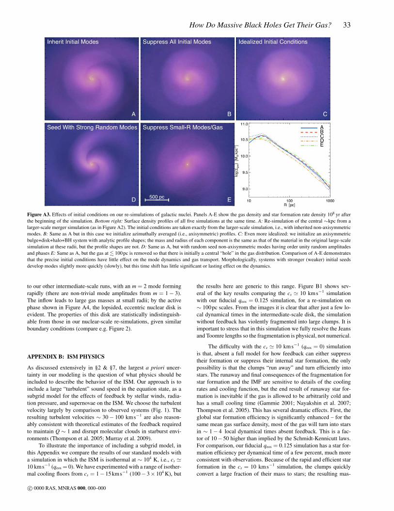
How Do Massive Black Holes Get Their Gas? 33
Figure A3. Effects of initial conditions on our re-simulations of galactic nuclei. Panels A-E show the gas density and star formation rate density 108 yr afterthe beginning of the simulation. Bottom right: Surface density profiles of all five simulations at the same time. A: Re-simulation of the central ∼kpc from alarger-scale merger simulation (as in Figure A2). The initial conditions are taken exactly from the larger-scale simulation, i.e., with inherited non-axisymmetricmodes. B: Same as A but in this case we initialize azimuthally averaged (i.e., axisymmetric) profiles. C: Even more idealized: we initialize an axisymmetricbulge+disk+halo+BH system with analytic profile shapes; the mass and radius of each component is the same as that of the material in the original large-scalesimulation at these radii, but the profile shapes are not. D: Same as A, but with random seed non-axisymmetric modes having order unity random amplitudesand phases E: Same as A, but the gas at . 100pc is removed so that there is initially a central “hole” in the gas distribution. Comparison of A-E demonstratesthat the precise initial conditions have little effect on the mode dynamics and gas transport. Morphologically, systems with stronger (weaker) initial seedsdevelop modes slightly more quickly (slowly), but this time shift has little significant or lasting effect on the dynamics.
to our other intermediate-scale runs, with an m = 2 mode formingrapidly (there are non-trivial mode amplitudes from m = 1− 3).The inflow leads to large gas masses at small radii; by the activephase shown in Figure A4, the lopsided, eccentric nuclear disk isevident. The properties of this disk are statistically indistinguish-able from those in our nuclear-scale re-simulations, given similarboundary conditions (compare e.g. Figure 2).
APPENDIX B: ISM PHYSICS
As discussed extensively in §2 & §7, the largest a priori uncer-tainty in our modeling is the question of what physics should beincluded to describe the behavior of the ISM. Our approach is toinclude a large “turbulent” sound speed in the equation state, as asubgrid model for the effects of feedback by stellar winds, radia-tion pressure, and supernovae on the ISM. We choose the turbulentvelocity largely by comparison to observed systems (Fig. 1). Theresulting turbulent velocities ∼ 30− 100 kms−1 are also reason-ably consistent with theoretical estimates of the feedback requiredto maintain Q ∼ 1 and disrupt molecular clouds in starburst envi-ronments (Thompson et al. 2005; Murray et al. 2009).
To illustrate the importance of including a subgrid model, inthis Appendix we compare the results of our standard models witha simulation in which the ISM is isothermal at ∼ 104 K, i.e., cs '10 kms−1 (qeos = 0). We have experimented with a range of isother-mal cooling floors from cs = 1− 15kms−1 (100− 3× 10⁴ K), but
the results here are generic to this range. Figure B1 shows sev-eral of the key results comparing the cs ' 10 kms−1 simulationwith our fiducial qeos = 0.125 simulation, for a re-simulation on∼ 100pc scales. From the images it is clear that after just a few lo-cal dynamical times in the intermediate-scale disk, the simulationwithout feedback has violently fragmented into large clumps. It isimportant to stress that in this simulation we fully resolve the Jeansand Toomre lengths so the fragmentation is physical, not numerical.
The difficulty with the cs ' 10 kms−1 (qeos = 0) simulationis that, absent a full model for how feedback can either suppresstheir formation or suppress their internal star formation, the onlypossibility is that the clumps “run away” and turn efficiently intostars. The runaway and final consequences of the fragmentation forstar formation and the IMF are sensitive to details of the coolingrates and cooling function, but the end result of runaway star for-mation is inevitable if the gas is allowed to be arbitrarily cold andhas a small cooling time (Gammie 2001; Nayakshin et al. 2007;Thompson et al. 2005). This has several dramatic effects. First, theglobal star formation efficiency is significantly enhanced – for thesame mean gas surface density, most of the gas will turn into starsin ∼ 1− 4 local dynamical times absent feedback. This is a fac-tor of 10−50 higher than implied by the Schmidt-Kennicutt laws.For comparison, our fiducial qeos = 0.125 simulation has a star for-mation efficiency per dynamical time of a few percent, much moreconsistent with observations. Because of the rapid and efficient starformation in the cs = 10 kms−1 simulation, the clumps quicklyconvert a large fraction of their mass to stars; the resulting mas-
c© 0000 RAS, MNRAS 000, 000–000
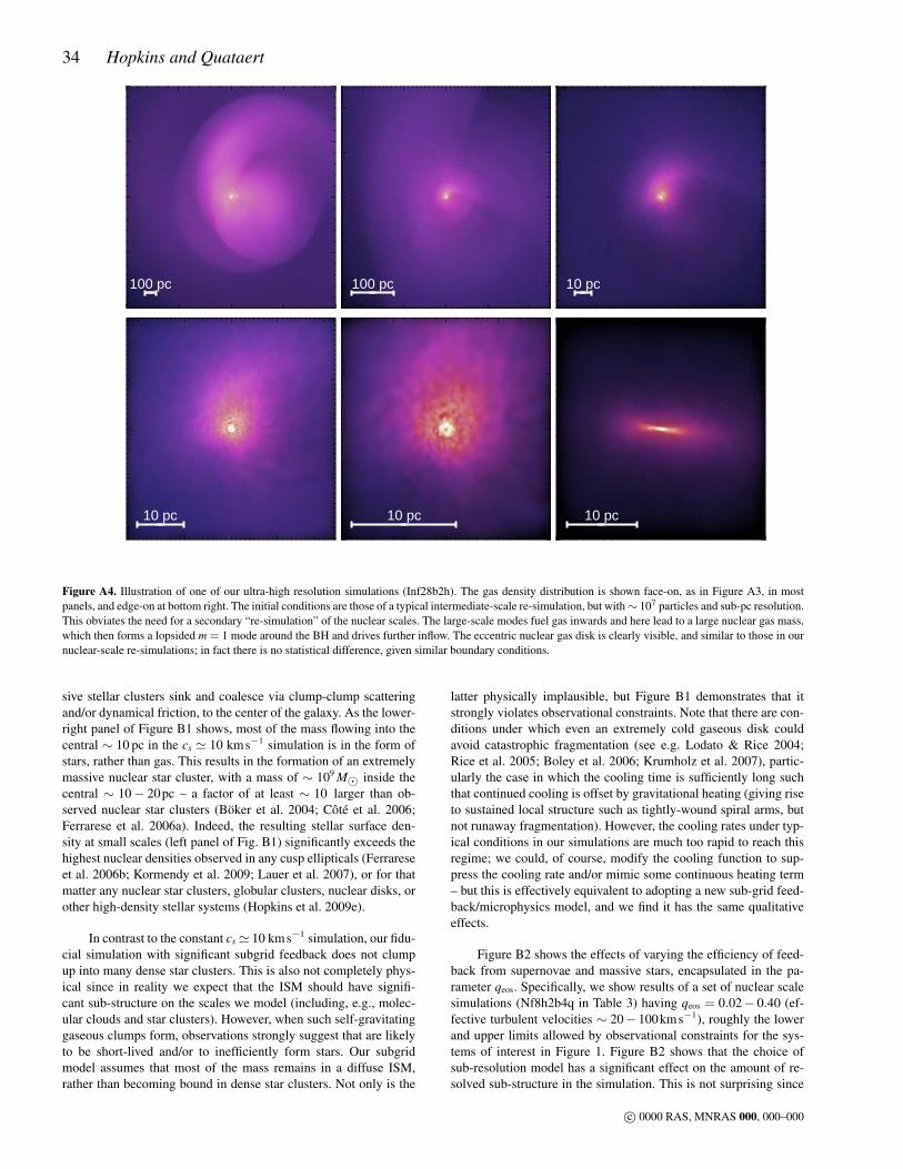
34 Hopkins and Quataert
100 pc
100 pc
10 pc
10 pc
10 pc
10 pc
Figure A4. Illustration of one of our ultra-high resolution simulations (Inf28b2h). The gas density distribution is shown face-on, as in Figure A3, in mostpanels, and edge-on at bottom right. The initial conditions are those of a typical intermediate-scale re-simulation, but with∼ 107 particles and sub-pc resolution.This obviates the need for a secondary “re-simulation” of the nuclear scales. The large-scale modes fuel gas inwards and here lead to a large nuclear gas mass,which then forms a lopsided m = 1 mode around the BH and drives further inflow. The eccentric nuclear gas disk is clearly visible, and similar to those in ournuclear-scale re-simulations; in fact there is no statistical difference, given similar boundary conditions.
sive stellar clusters sink and coalesce via clump-clump scatteringand/or dynamical friction, to the center of the galaxy. As the lower-right panel of Figure B1 shows, most of the mass flowing into thecentral ∼ 10 pc in the cs ' 10 kms−1 simulation is in the form ofstars, rather than gas. This results in the formation of an extremelymassive nuclear star cluster, with a mass of ∼ 109 M inside thecentral ∼ 10− 20pc – a factor of at least ∼ 10 larger than ob-served nuclear star clusters (Böker et al. 2004; Côté et al. 2006;Ferrarese et al. 2006a). Indeed, the resulting stellar surface den-sity at small scales (left panel of Fig. B1) significantly exceeds thehighest nuclear densities observed in any cusp ellipticals (Ferrareseet al. 2006b; Kormendy et al. 2009; Lauer et al. 2007), or for thatmatter any nuclear star clusters, globular clusters, nuclear disks, orother high-density stellar systems (Hopkins et al. 2009e).
In contrast to the constant cs ' 10 kms−1 simulation, our fidu-cial simulation with significant subgrid feedback does not clumpup into many dense star clusters. This is also not completely phys-ical since in reality we expect that the ISM should have signifi-cant sub-structure on the scales we model (including, e.g., molec-ular clouds and star clusters). However, when such self-gravitatinggaseous clumps form, observations strongly suggest that are likelyto be short-lived and/or to inefficiently form stars. Our subgridmodel assumes that most of the mass remains in a diffuse ISM,rather than becoming bound in dense star clusters. Not only is the
latter physically implausible, but Figure B1 demonstrates that itstrongly violates observational constraints. Note that there are con-ditions under which even an extremely cold gaseous disk couldavoid catastrophic fragmentation (see e.g. Lodato & Rice 2004;Rice et al. 2005; Boley et al. 2006; Krumholz et al. 2007), partic-ularly the case in which the cooling time is sufficiently long suchthat continued cooling is offset by gravitational heating (giving riseto sustained local structure such as tightly-wound spiral arms, butnot runaway fragmentation). However, the cooling rates under typ-ical conditions in our simulations are much too rapid to reach thisregime; we could, of course, modify the cooling function to sup-press the cooling rate and/or mimic some continuous heating term– but this is effectively equivalent to adopting a new sub-grid feed-back/microphysics model, and we find it has the same qualitativeeffects.
Figure B2 shows the effects of varying the efficiency of feed-back from supernovae and massive stars, encapsulated in the pa-rameter qeos. Specifically, we show results of a set of nuclear scalesimulations (Nf8h2b4q in Table 3) having qeos = 0.02− 0.40 (ef-fective turbulent velocities ∼ 20− 100kms−1), roughly the lowerand upper limits allowed by observational constraints for the sys-tems of interest in Figure 1. Figure B2 shows that the choice ofsub-resolution model has a significant effect on the amount of re-solved sub-structure in the simulation. This is not surprising since
c© 0000 RAS, MNRAS 000, 000–000
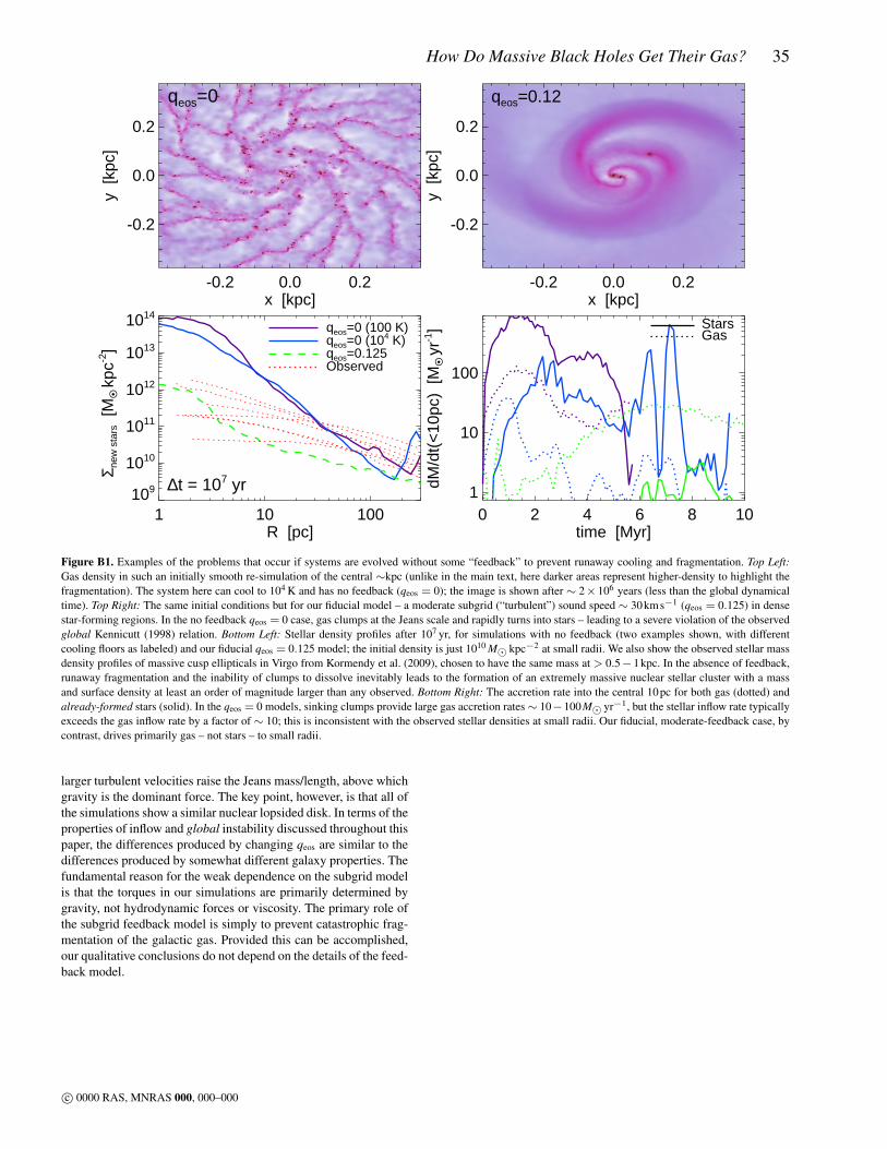
How Do Massive Black Holes Get Their Gas? 35
-0.2 0.0 0.2x [kpc]
-0.2
0.0
0.2y
[kpc
]qeos=0
-0.2 0.0 0.2x [kpc]
-0.2
0.0
0.2
y [k
pc]
qeos=0.12
1 10 100R [pc]
109
1010
1011
1012
1013
1014
Σ new
sta
rs [
MO • k
pc-2]
qeos=0 (100 K)qeos=0 (104 K)qeos=0.125Observed
∆t = 107 yr
0 2 4 6 8 10time [Myr]
1
10
100
dM/d
t(<
10pc
) [M
O • y
r-1] Stars
Gas
Figure B1. Examples of the problems that occur if systems are evolved without some “feedback” to prevent runaway cooling and fragmentation. Top Left:Gas density in such an initially smooth re-simulation of the central ∼kpc (unlike in the main text, here darker areas represent higher-density to highlight thefragmentation). The system here can cool to 104 K and has no feedback (qeos = 0); the image is shown after ∼ 2× 10⁶ years (less than the global dynamicaltime). Top Right: The same initial conditions but for our fiducial model – a moderate subgrid (“turbulent”) sound speed ∼ 30kms−1 (qeos = 0.125) in densestar-forming regions. In the no feedback qeos = 0 case, gas clumps at the Jeans scale and rapidly turns into stars – leading to a severe violation of the observedglobal Kennicutt (1998) relation. Bottom Left: Stellar density profiles after 107 yr, for simulations with no feedback (two examples shown, with differentcooling floors as labeled) and our fiducial qeos = 0.125 model; the initial density is just 1010 M kpc−2 at small radii. We also show the observed stellar massdensity profiles of massive cusp ellipticals in Virgo from Kormendy et al. (2009), chosen to have the same mass at > 0.5− 1kpc. In the absence of feedback,runaway fragmentation and the inability of clumps to dissolve inevitably leads to the formation of an extremely massive nuclear stellar cluster with a massand surface density at least an order of magnitude larger than any observed. Bottom Right: The accretion rate into the central 10pc for both gas (dotted) andalready-formed stars (solid). In the qeos = 0 models, sinking clumps provide large gas accretion rates∼ 10−100M yr−1, but the stellar inflow rate typicallyexceeds the gas inflow rate by a factor of ∼ 10; this is inconsistent with the observed stellar densities at small radii. Our fiducial, moderate-feedback case, bycontrast, drives primarily gas – not stars – to small radii.
larger turbulent velocities raise the Jeans mass/length, above whichgravity is the dominant force. The key point, however, is that all ofthe simulations show a similar nuclear lopsided disk. In terms of theproperties of inflow and global instability discussed throughout thispaper, the differences produced by changing qeos are similar to thedifferences produced by somewhat different galaxy properties. Thefundamental reason for the weak dependence on the subgrid modelis that the torques in our simulations are primarily determined bygravity, not hydrodynamic forces or viscosity. The primary role ofthe subgrid feedback model is simply to prevent catastrophic frag-mentation of the galactic gas. Provided this can be accomplished,our qualitative conclusions do not depend on the details of the feed-back model.
c© 0000 RAS, MNRAS 000, 000–000
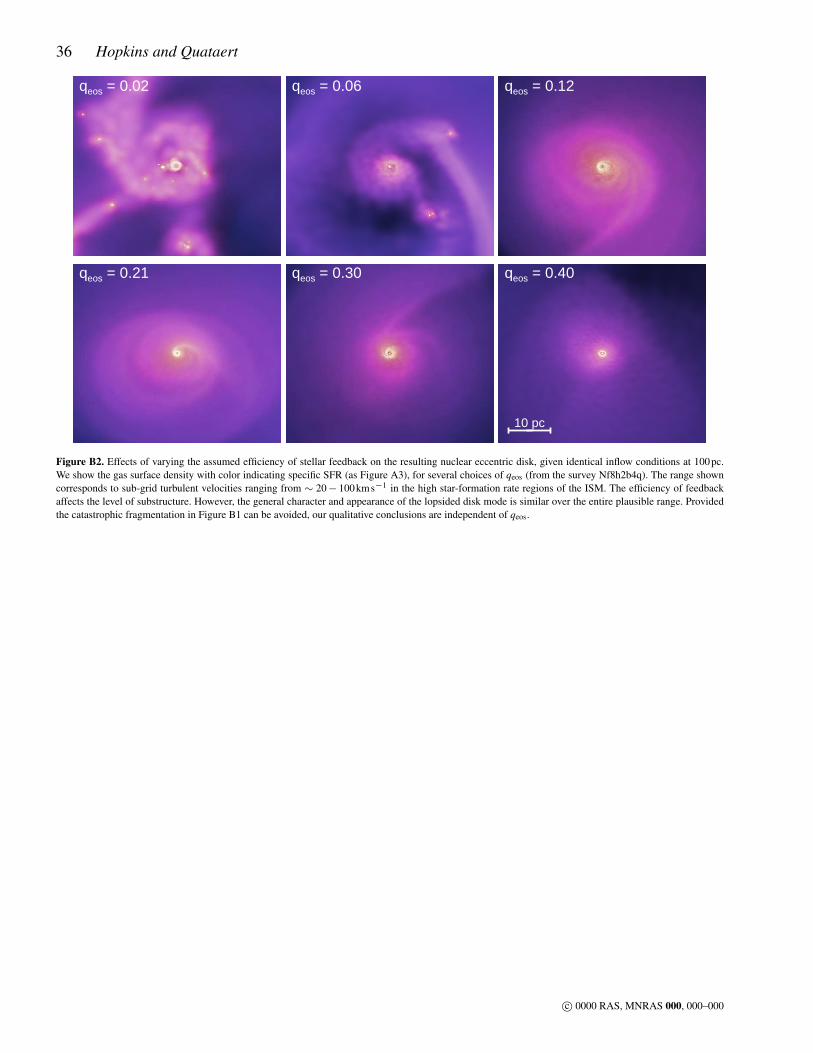
36 Hopkins and Quataert
qeos = 0.02 qeos = 0.06 qeos = 0.12
qeos = 0.21 qeos = 0.30 qeos = 0.40
10 pc
Figure B2. Effects of varying the assumed efficiency of stellar feedback on the resulting nuclear eccentric disk, given identical inflow conditions at 100pc.We show the gas surface density with color indicating specific SFR (as Figure A3), for several choices of qeos (from the survey Nf8h2b4q). The range showncorresponds to sub-grid turbulent velocities ranging from ∼ 20− 100kms−1 in the high star-formation rate regions of the ISM. The efficiency of feedbackaffects the level of substructure. However, the general character and appearance of the lopsided disk mode is similar over the entire plausible range. Providedthe catastrophic fragmentation in Figure B1 can be avoided, our qualitative conclusions are independent of qeos.
c© 0000 RAS, MNRAS 000, 000–000