HOUSEHOLDS’ WATER USE DEMAND AND WILLINGNESS

TO PAY FOR IMPROVED WATER SERVICES: A CASE STUDY

OF SEMI-URBAN AREAS IN THE LUBOMBO AND LOWVELD

REGIONS OF SWAZILAND

By

NQOBIZWE MVANGELI DLAMINI

BSc. (Agri-Econ & Agri-Business), Swaziland

A THESIS SUBMITTED TO THE FACULTY OF DEVELOPMENT STUDIES

IN PARTIAL FULFILLMENT OF THE REQUIREMENTS FOR THE

AWARD OF THE DEGREE OF MASTER OF SCIENCE IN

AGRICULTURAL AND APPLIED ECONOMICS

LILONGWE UNIVERSITY OF AGRICULTURE AND NATURAL

RESOURCES (LUANAR), BUNDA CAMPUS

DEPARTMENT OF AGRICULTURAL AND APPLIED ECONOMICS

OCTOBER 2015

ii

DECLARATION

I, Nqobizwe Mvangeli Dlamini, declare that this thesis is a result of my own original

effort and work, and that to the best of my knowledge, the findings have never been

previously presented to Lilongwe University of Agriculture and Natural Resources

(LUANAR) or elsewhere for the award of any academic qualification. Where

assistance was sought, it has been accordingly acknowledged.

Nqobizwe Mvangeli Dlamini

Signature: _________________________________

Date: __________________________________

iii

CERTIFICATE OF APPROVAL

We, the undersigned, certify that this thesis is a result of the author‟s own work, and

that to the best of our knowledge, it has not been submitted for any other academic

qualification within Lilongwe University of Agriculture and Natural Resources or

elsewhere. The thesis is acceptable in form and content, and that satisfactory

knowledge of the field covered by the thesis was demonstrated by the candidate

through an oral examination held on 6th

October, 2015.

Major Supervisor: Professor Abdi K. Edriss

Signature: ______________________________

Date: ______________________________

Supervisor: Dr. Charles B. L. Jumbe

Signature: ______________________________

Date: ______________________________

Supervisor: Professor Micah B. Masuku

Signature: ______________________________

Date: ______________________________

iv

DEDICATION

This thesis is dedicated to my mother, Maggie Maphako and my late father, Zebron

Dlamini (R.I.P).

v

ACKNOWLEDGMENTS

First and foremost, I would love to thank God, the father of my Lord Jesus Christ for

showing me favour before his eyes. I do believe that without his loving and forgiving

mercy I wouldn‟t have made it this far.

I would also like to acknowledge the contributions of the following, for which without

their inputs I would have not completed this work; my sponsor, African Economic

Research Consortium (AERC), for providing the necessary funding for my studies.

Many thanks also go to my supervisor, Professor A. K. Edriss, for his patience,

constant support and excellent guidance during my graduate studies at Lilongwe

University of Agriculture and Natural Resources (LUANAR). Likewise, I owe many

thanks to my co-supervisor, Dr. Charles B. L. Jumbe, Associate Professor, for his

patience, guidance, enthusiastic encouragement and useful critiques of this thesis

work. I would also like to extend my sincere gratitude to my other co-supervisor, Dr.

M. B. Masuku, Associate Professor and Dean in the University of Swaziland faculty

of Agriculture and Consumer Sciences. I am very grateful for his patience in nurturing

me as a young man to what I have become. He believed in me even when I couldn‟t

believe in myself. For that, I am grateful and will forever cherish.

Many thanks to Dr. M.A.R. Phiri, Head of Department for Agricultural and Applied

Economics in LUANAR, for affording me the opportunity to undertake my studies

here at LUANAR. Many thanks also go to my other teachers and staff at LUANAR,

Dr. L. P. Mapemba, Dr. M. Mwabumba and Prof. D.H.N. Ngongola, for providing me

with a strong base in the field of economics. To all the other members of staff in

LUANAR, from house cleaners, secretaries, drivers and accountants, am very grateful

vi

for making my two year stay here in LUANAR a memorable one. Indeed, through

your humility, Malawi is “the warm heart of Africa”.

I would also like to extent my thanks to Mr. B. Mdluli, from the Swaziland Water

Services Cooperation (SWSC), Mr. S. Francesca from the European Union (EU)

offices in Swaziland and Mrs. N. Ntshalintshali, from the Department of Water

Affairs (DWA) for their assistance with relevant information used in the study.

Finally, I am indebted to pass my gratitude to my entire family; my mother, my sister,

my brothers, nephews and nieces for their words of encouragement and spiritual and

financial support. Their mere existence made it possible for me not to give up even

when the going got tough.

vii

TABLE OF CONTENTS

DECLARATION...................................................................................................................... ii

CERTIFICATE OF APPROVAL ........................................................................................ iii

DEDICATION......................................................................................................................... iv

ACKNOWLEDGMENTS ....................................................................................................... v

LIST OF TABLES ................................................................................................................... x

LIST OF FIGURES ................................................................................................................. x

LIST OFABBREVIATIONS AND ACRONYMS ............................................................... xi

ABSTRACT .......................................................................................................................... xiii

CHAPTER ONE ...................................................................................................................... 1

INTRODUCTION.................................................................................................................... 1

1.1 Background ...................................................................................................................... 1

1.2 Problem Statement ........................................................................................................... 4

1.3 Objectives ......................................................................................................................... 6

1.4 Hypotheses ....................................................................................................................... 6

1.5 Research Questions .......................................................................................................... 7

1.6 Justification ...................................................................................................................... 8

1.7 Organisation of the Study ................................................................................................. 9

CHAPTER TWO ................................................................................................................... 10

LITERATURE REVIEW ..................................................................................................... 10

2.1 Valuation of Natural Resources ..................................................................................... 10

2.2 Theory of Welfare Change ............................................................................................. 11

2.3 Contingent Valuation Method (CVM) ........................................................................... 16

2.3.1 Contingency Valuation Formats .................................................................. 18

2.3.2 Contingency Valuation Biases..................................................................... 21

viii

2.4 Empirical CVM literature on water ................................................................................ 24

2.5 Empirical literature on water demand in developing countries ...................................... 29

2.6 Concluding Summary ..................................................................................................... 32

CHAPTER THREE ............................................................................................................... 33

METHODOLOGY ................................................................................................................ 33

3.1 Conceptual Framework .................................................................................................. 33

3.2 Theoretical Framework .................................................................................................. 35

3.3 Empirical Framework ..................................................................................................... 38

3.3.1 Estimating mean willingness to pay ............................................................ 38

3.3.2 Factors affecting willingness to pay ............................................................ 41

3.3.3 Factors affecting household water consumption ......................................... 46

3.4 Description of variables and expected outcomes ........................................................... 48

3.4.1 Dependent Variables .................................................................................... 48

3.4.2 Independent Variables ................................................................................. 49

3.5 Study Area ...................................................................................................................... 54

3.6 Sampling Technique and Sample Size ........................................................................... 54

3.7 Data and Collection Methods ......................................................................................... 56

3.8 Designing and Administering the Contingent Valuation Survey ................................... 58

CHAPTER FOUR .................................................................................................................. 60

RESULTS AND DISSCUSSION .......................................................................................... 60

4.1 Descriptive Statistics ...................................................................................................... 60

4.1.1 Socio-Economic Characteristics of Households .......................................... 60

4.1.2 Household Water Use Attributes and Perceptions ...................................... 64

4.2 Willingness to Pay Estimation ....................................................................................... 67

ix

4.2.1 Reasons for Maximum Willingness to Pay ................................................. 71

4.3 Estimation of Parametric Mean from Double Bounded Dichotomous Choice

Format .................................................................................................................................. 72

4.4 Determinants of Willingness to Pay ............................................................................... 74

4.5 Factors affecting household water consumption ............................................................ 82

CHAPTER FIVE ................................................................................................................... 88

SUMMARY OF FINDINGS, CONCLUSIONS AND RECOMMENDATIONS ............ 88

5.1 Summary of findings ...................................................................................................... 88

5.2 Conclusions .................................................................................................................... 89

5.3 Recommendations .......................................................................................................... 91

5.4 Areas of Further Research .............................................................................................. 92

REFERENCES ....................................................................................................................... 94

APPENDIX I: SURVEY QUESTIONNAIRE................................................................... 106

APPENDIX II: VIF Stata output for Explanatory Variables used in Probit

Model ..................................................................................................................................... 116

APPENDIX III: Stata results for Ramsey Specification Test for LPM .......................... 116

APPENDIX IV: Contingency Coefficient for Discrete Variables ................................... 116

APPENDIX V: VIF Stata output for Explanatory Variables used in Double-log

Model ..................................................................................................................................... 117

APPENDIX VI: Stata output for Ramsey Specification Test for Double-log

Regression ............................................................................................................................. 117

APPENDIX VII: Stata output for Heteroskedaticty Test for Double-log

Regression ............................................................................................................................. 118

x

LIST OF TABLES

Table 3.1 Summary of Sampled Households ......................................................................... 56

Table 4.1 Sex Composition of Sample Households ............................................................... 61

Table 4.2 Age, Household Size, Income, Distance and Education of Households ............... 62

Table 4.3 Source of water for sampled Households ............................................................... 64

Table 4.4 Water Consumption, Time Spent, Expenditure and Trips of Households ............. 67

Table 4.5 Summary of Discrete Response to the Double-Bounded Questions ..................... 69

Table 4.6 Frequency of Joint Willingness to Pay questions .................................................. 70

Table 4.7 Reasons for Willingness to Pay .............................................................................. 71

Table 4.8 Reasons for Not Willing To Pay ............................................................................ 72

Table 4.9 Descriptive Statistics of the Dichotomous Choice Format .................................... 73

Table 4.10 Estimates of the Bivariate Probit Model .............................................................. 74

Table 4.11 Probit and Marginal Effect Results for Willingness to Pay ................................. 76

Table 4.12 Double-log Regression Analysis for Water Demand Determinants .................... 84

LIST OF FIGURES

Figure 3.1 Conceptual Framework for Improved Water Services ......................................... 34

Figure 4.1 Pilot survey results on WTP ................................................................................. 68

xi

LIST OFABBREVIATIONS AND ACRONYMS

ABM Averting Behaviour Method

CBA Cost Benefit Analysis

CS Consumer Surplus

CSO Central Statistics Office

CSU Compensating Surplus

CV Compensating Variation

CVM Contingency Valuation Method

DBDC Double-Bounded Dichotomous Choice

E Emalangeni

ESU Equivalent Surplus

EU European Union

EV Equivalent Variation

GOS Government of Swaziland

HPM Hedonic Pricing Method

IIED International Institute for Environment and

Development

IWRM Integrated Water Resource Management

MGD Millennium Development Goals

SWSC Swaziland Water Services Cooperation

xii

TCM Travel Cost Method

UNDP United Nation Development Programme

VAC Vulnerability Assessment Committee

WTA Willingness to Accept

WTP Willingness to Pay

xiii

ABSTRACT

This study was designed to assess household water demand and willingness to pay

(WTP) for improved water services in the Lowveld and Lubombo regions of

Swaziland. Using both purposive and cluster sampling methods, survey data were

collected from 314 households in the month of April 2015, mainly in three

constituencies, namely; Siphofaneni, Matsanjeni and Somnongtongo. The study used

the Contingent Valuation Method (CVM) to estimate WTP using a double bounded

dichotomous choice elicitation format. In assessing the determinants of WTP and

water consumption, the study employed both the probit model and double-log

regression model, respectively. Results from the study showed that about 67% of

households in the study areas were willing to pay the initial bid offered for an

improvement in their water services. Generally, about 93% of the sampled households

were willing to pay something for the improvement in water services. The study

further showed that the estimated mean WTP for a 20 litre of water was E0.471. On

household water demand, results showed that the mean daily per capita water

consumption was 13.12 litres. Results from the probit model showed that household

income, education, gender, distance and owning a backyard garden positively and

significantly affect WTP. Furthermore, age, water quality and the initial bid offered

negatively and significantly affected WTP for improved water. On the other hand,

results from the double-log regression model showed that education, household

income and ownership of a water tank were positive factors influencing household

water consumption. In addition, household size, distance and years of using source

were negative determinants of household water consumption. The implications of the

study are that factors such as age, income, level of education, gender, distance and

1 1 USD = E13.5 Emalangeni

xiv

household size should be considered when setting domestic water tariffs and

designing strategies on demand management.

1

CHAPTER ONE

INTRODUCTION

1.1 Background

The provision of safe and clean water to the rural and semi-urban areas of Swaziland

holds an enormous potential of uplifting livelihoods. As pointed by Okun (1988),

improved access to clean and safe water supply is closely linked to improved

economic wellbeing. The clear interdependence between water availability and

development is exemplified by the link between water and poverty (Coster and

Otufale, 2014). Similarly, the Swaziland Poverty Reduction Strategy and Action Plan

(PRSAP) identified the inefficient access to safe and clean water as the core cause of

poverty in Swaziland, which has to be addressed immediately (Government of

Swaziland [GoS], 2007). According to the 2013 annual Vulnerability Assessment

Committee (VAC) report, it is estimated that about 62% and 64% of the total

population have access to improved water sources during dry and rainy seasons,

respectively (GoS, 2013). In line with Millennium Development Goal (MDG) number

7 and national targets, the country aspires to supply all communities with clean water

by 2015 and as well as safe, affordable and acceptable drinking water for all by 2022

(Nazarene Compassionate Ministries [NCM], 2013).

However, water resources in recent years have been under stress owing to substantial

growth in human populations (International Institute for Environment and

Development [IIED], 2012). Increases in human populations imply substantial

increases in the demand for food and other social services. This has been no different

to Swaziland as a number of scholars have recognized that local water supply is

beyond sustainable supply (Peter and Nkambule, 2012; Farolfi et al., 2007). In a

2

resource economics perspective, the water resource is being over extracted, while it is

also not being efficiently allocated. For the same reason, economists have been

advocating the idea of attaching a monetary value to water which potentially can

improve sustainable use (Hanemann, 1994; Chandrasekaran et al., 2009) and thus

maximise economic and social welfare in an equitable manner.

According to Pearce (1993), important conservational strategies and projects are

rightfully addressed when monetary prices are identified. However, in contrast,

traditionally water in rural communities has been assessed as a non-market good from

natural sources like rivers, wells, lakes and dams, which are shared by both humans

and animals. This usage amid of population pressures has had severe implications not

only on humans but also on the environment. Water degradation and contamination

have resulted mainly because of over exploitation, and because of poor sanitation,

ground water gets contaminated too. Such situation has left most households to rely

on government-provided community water schemes to supply clean water to the rural

and semi-urban populations. This reliance has been further exuberated as some of the

traditional sources have run dry or contaminated leaving rural residents to travel long

distances for water.

Swaziland is divided into four ecological zones: the Highveld, Middleveld, Lowveld

and Lubombo Plateau. Due to droughts in recent years, many areas of the country are

facing aggravated water scarcity. The dry parts of the Lowveld and Lubombo regions

are examples of such areas where water scarcity has inflicted injuries on the social

and economic lives of the populace (Mijinyawa and Dlamini, 2008). As a result,

government efforts to supply water through community taps or boreholes have

3

focused mainly in these areas in recent years (GoS, 2013). These efforts, however,

have not been successful mainly because water discharged from these sources are of

very low quantities and the sources get desiccated during dry seasons (Mijinyawa and

Dlamini, 2008). Moreover, where these sources are relatively reliable, water produced

is of compromised quality. These communities rely only on these sources as their

main primary source of potable water and the secondary source of buying water from

water vendors at inflated prices further pushes them to a severe poverty trap.

To address this problem, the European Union (EU) through the Government of

Swaziland (GoS) and Swaziland Water Service Cooperation (SWSC) has funded a

water project to supply communities in these areas, mainly in Matsanjeni,

Somnotongo and Siphofaneni, with clean treated water and sanitation services

through commercialization of water services. Water will be sold in kiosks for

households that cannot afford a private water connection, while those affording,

private connection will be made and meters installed for monthly payments. However,

a socially acceptable price to be charged relative to these communities is unknown as

this is a project of its first kind in rural communities. The importance of setting a

„socially efficient‟ price is justified by the fact that an exaggerated price of water can

further push households to severe poverty while a very low price can cause

unsustainable demand to water, a resource already under stress.

As such, a thorough investigation on the extent to which households are willing to pay

for improved water services and the amount they are willing to pay is of great

importance. Firstly, such knowledge will enhance water managers to understand the

demand side for improved water services in these areas. Secondly, this will allow

4

water managers to know if households in the study areas are capable of paying a price

of water which can ensure sustainability of the project without compromising rural

livelihoods. Lastly, this can also help policy makers in setting targeted subsidies on

poor households. Therefore, the purpose of this study is to estimate Willingness to

Pay (WTP) for improved water services and household water demand in the semi-

urban areas of the Lubombo and Shiselweni regions, which can potentially improve

the understanding of the demand side for improved water services in these areas.

1.2 Problem Statement

Most rural households spend a lot of time collecting water due to non-functioning of

community water schemes. This forces poor households to travel long distances to

access water from unhealthy sources like wells and rivers (Mijinyawa and Dlamini,

2008). Where functional, queues are an inevitable problem as these water projects

supply quite a substantial number of households. Such long queues divert valuable

time from numerous economically productive activities for the poor (IIED, 2009).

Also as noted by Ainuson (2009), staying in long queues for a long time at water

provision centres is a source of tension and often leads into conflicts. Such conditions

force these poor households to use unsafe alternatives of water sources like rivers and

dams. Consequently, this result in high levels of water borne diseases and hygiene

problems, which leads to high mortality rates, increased health costs and reduced

labour productivity to the poor.

The idea of a potential Pareto improvement thus provides the rationale for public

intervention to increase the efficiency of resource allocation (Haab and McConnell,

2002). Therefore, the government and affected parties are faced with an urgent task of

5

supplying clean water to rural communities in an effort to uplift rural livelihoods.

Decisions on water allocation in Swaziland, however, are currently taken on the basis

of very limited information. Thus, environmental valuation attempts to quantify the

benefits of environmental or public projects and policies, so that they are more

transparent, and can be given due and appropriate weight in any decision making

process or cost benefit analysis (CBA) (Garrod and Willis, 1999). Based on resource

economics theory, government is justified to provide improved water services if the

unit cost of establishing one is equal or less than the value the community attach to

such a service.

However, lack of knowledge on rural household‟s WTP for water services exists in

the rural areas of Swaziland. This further discourages both government and private

interest on establishing more water sources as there is no evidence whether such

projects can be successful or sustainable. Moreover, these community water projects

put pressure on government expenditures making government unable to expand water

supply to other equally poor communities facing aggravated water scarcity. Therefore,

as noted by Kanyoka et al. (2008), financially viable rural water projects should come

as a form of partial coverage from communities through the introduction of water

fees. It is, therefore, important to determine the non-market value rural communities

attach to such water services for efficient resource allocation.

As already stated, there exists a negligible literature on households WTP for

household water and water demand in Swaziland. Most researchers have been

focusing on the impacts and sustainability factors of community water schemes (Peter

and Nkambule, 2012; Ndwandwe, 2005; Manyatsi and Mwendera, 2007). According

6

to the author‟s knowledge, a study by Farolfi et al. (2007) estimated domestic water

use and values in Swaziland. However, as pointed out by a number of researchers,

WTP for water varies from time to time and from location to location (Rogerson,

1996; Gunatilake and Tachiiri, 2012). Therefore, the study aims at estimating WTP

for improved water services in the semi-urban areas of Swaziland which is important

for evaluating policy alternatives, setting socially acceptable water tariffs and for cost

recovery purposes.

1.3 Objectives

The main objective of the study is to estimate willingness to pay for improved water

services among households in the study areas.

The specific objectives of the study are to:

i. Quantify WTP for improved water services and household water use demand.

ii. Estimate the parametric mean WTP for improved water services.

iii. Determine the factors affecting WTP for improved water service.

iv. Assess the factors affecting per capita water consumption.

1.4 Hypotheses

Based on a survey of literature the study forms the following hypotheses;

i. Households without a nearby or private water source do not have a higher

WTP than their counterparts with such.

7

ii. Similarly, households who travel shorter distances to collect water do not

consume more water per capita than their counterfactuals that travel longer

distances.

iii. Households with higher incomes will not demand more improved water

services as they are probably consuming such. Therefore, it is hypothesised

that income will affect WTP negatively.

iv. Socio-economic variables like age, education, household size, gender, marital

status and social position, do not affect households‟ WTP for improved water

services and household water consumption.

v. Households which already have enough water have no incentive to pay more

for improvement in quantity. That is, households already consuming higher

levels of water may not be willing to pay for an improvement in their water

services.

1.5 Research Questions

The study aims at answering the following questions:

i. Are households in the study areas willing to pay for improved water services

and how much are they willing to pay?

ii. What factors influence household per capita water consumption and WTP for

improved water services in the study areas?

8

1.6 Justification

A more comprehensive knowledge of the structure of water demand both through

survey utility data and stated preference methods can help to better understand

consumer behaviour. As noted by Nauges and Whittington (2010), management of

water resources in an equitable manner by water managers has proved to be a

demanding task. Therefore, evaluating domestic water demand behaviours produces

an underlying basis for water managers to sustainably and efficiently meet the ever

increasing demand for water. Likewise, knowledge on how socio-economic

characteristics influence responsiveness of water demand to price and non-price

factors provides appropriate policy information on household demand characteristics

(Strand and Walker, 2005).

As such, Swaziland‟s „Vision 2022‟ with respect to the water sector seeks to attain a

100% supply of safe, affordable and acceptable drinking water for all. Achieving such

a goal requires relevant information regarding households‟ water demand behaviours

and the factors that influence WTP for improved water services. As noted by

Whittington et al. (1991), it is important to conduct studies which help in

understanding water use and its dynamics at household level as it enhances informed

decision making amongst water managers. This study is, therefore, timely and can

contribute in achieving the targets set for water coverage by providing relevant

household level information.

Furthermore, in light of the proposed EU water project, the unavailability of

information on households WTP for improved water services and water demand

characteristics in the study areas further justified the need to conduct the study. The

9

study will potentially contribute in setting a socially acceptable price and further

provide an understanding on the demand for household water in these areas. It is,

however, worth mentioning that WTP is not a measure for price (Banda et al., 2006).

However, the results from the study can be used in CBA when determining whether

the project is worth implementing (Bateman et al., 2002). Therefore, the study aims to

assess households‟ WTP for improved water services and water demand in an effort

to provide important information for improving water accessibility.

1.7 Organisation of the Study

The study is organized into five chapters. After this chapter, Chapter two provides an

extensive review of literature, from the theoretical foundations of welfare change to

reviews of related empirical literature on WTP for water services and household water

demand. Chapter three presents a detailed description of the conceptual, theoretical

and empirical frameworks adopted in the study. The chapter also includes a

description of the study areas, sampling size and sampling techniques adopted.

Chapter four presents descriptive analysis from the survey data and also discusses the

empirical findings of this study. Finally, chapter five presents a summary of findings,

conclusions and recommendations from the study.

10

CHAPTER TWO

LITERATURE REVIEW

2.1 Valuation of Natural Resources

Economic valuation of environmental and natural resources entails assessing the

preferences of society with regards to an environmental resource or public good. It is

a method used for assigning monetary value to the outcomes of choices about

policies, projects and programmes (Bateman et al., 2002). Valuation of natural and

environmental goods has grown importance in recent years. This has been mainly due

to efforts by governments to increase resource allocation efficiency and sustainability

in the face of increased human pressures. Moreover, natural resources are also

resources such as labour and capital; therefore, it is important that they are

appropriately and sustainably managed. According to Pearce (1993), important

conservational and sustainable strategies for natural resources and public projects are

rightfully addressed when economic values are identified.

Most natural resources and public goods are provided freely and thus have missing

markets. In light of missing markets, resources are mismanaged and inefficiently

allocated due values of goods and services being not revealed (Kadekodi, 2001). At

times where markets exist, inefficiencies may still occur due to improper regulated

markets. Water generally is one good which is under-priced due to its public good

characteristics. According to Whittington et al. (1991), such kinds of environmental or

public goods are the main causes of externalities. Consequently, markets cannot

efficiently allocate such goods with pervasive externalities, or for which property

rights are not clearly defined (Haab and McConnell, 2002). Therefore, in solving for

11

externalities, it is important that economic values are attached to such public goods.

Valuation of natural resources like water therefore, reveals the economic value or

benefits individuals derive from their services for proper management (Whittington,

1998).

There are quite a number of economic methods used in valuing public or

environmental goods and they specifically belong to two categories. In the first

category are those which depend on observed human behaviours and thus derive

inferences about preferences and economic values from such behaviours. The second

category is those which rely on stated or revealed preferences by individuals. The

main valuation techniques between these categories are hedonic and travel cost

methods for the first category and while the second category consist of choice

modelling and contingent valuation methods (Haab and McConnell, 2002). According

to Tietenberg and Lewis (2012), the first category represents those involving observed

behaviour and the second category as one involving hypothetical behaviour. Revealed

preference method includes Hedonic Price Method (HPM) and Travel Cost Method

(TCM) while stated preference includes the Contingent Valuation Method (CVM) and

Choice Modelling (CM). This study uses the CVM to evaluate the non-market value

of improved household water services.

2.2 Theory of Welfare Change

The basic foundation of the theory of welfare economics is to increase the wellbeing

of an economic agent or individual in any economic activity. Previously, most studies

have looked into the welfare effects of prices consumers pay for goods sold in the

12

market without much consideration on environmental goods. According to Mitchell

and Carson (1989), economic values of environmental goods are measured using their

effects on human welfare. Therefore, estimating economic values of environmental or

public goods is an attempt to measure the impact and/benefits these goods bring to

individual utilities.

Changes in environmental or public goods can affect people‟s welfare in any of the

following four different ways. Firstly, such changes can affect individuals through the

prices they pay for goods in the market. Secondly, this also can affect and cause

changes in the prices individuals pay for their factors of production. Thirdly,

environmental changes can also affect individuals through changes in quality and

quantities of other public goods. Finally, a change in environmental or public good

can induce changes in risks individuals face (Freeman, 2003). In the case of this

study, an improvement in community water services can lower money spent on

market goods such as those for averting behaviours. Secondly the water project can

also lower the price of water currently used for production purposes. Lastly, the

improvement can induce sanitary in the community thus improving clean scenery and

improved clean air which concurrently can lower the risks of infections and child

mortality.

The central concern on policy makers is to measure among alternative public resource

allocation decisions to improve social welfare. A more appropriate welfare measure

for policy in the provision of public goods or resource allocation is the use of Pareto

improvement, a gain to one person without making any other one worse off. The idea

of a Pareto improvement lies on the basis that overall benefits of a public intervention

13

should exceed the costs of that intervention. In this context, resource allocation can

achieve greater efficiency. According to Perman et al. (2003), an allocation of

resources is said to be efficient if it is not possible to make one or more persons better

off without making at least other person worse off, allocative efficiency. Likewise, an

allocation is inefficient if it is possible to improve one‟s welfare without worsening

anyone else. Thus, Pareto improvement is not a sufficient but a necessary condition

for achieving allocative efficiency in environmental or public provisions of goods, a

state where no further improvements are possible without worsening ones welfare.

Conventionally, welfare changes from changes in environmental or public goods have

been estimated using Consumer Surplus (CS), the area under the Marshallian

(ordinary) demand curve above the price level. These demand functions are derived

through utility maximization. Consumers are presented with a problem of maximizing

utility subject to an income constraint. Solving the utility maximization problem leads

to a set of ordinary demand functions as functions of prices and income.

There have, however, been concerns about the use of CS as a welfare measure due its

inefficiency in keeping utility constant. In addition, environmental (or public) goods

have a particular characteristic that makes the concept of the Marshallian demand

function and CS difficult to be applied. The absence of a price for environmental or

public goods makes them untradeable as they do not have private property

characteristics. Therefore, one cannot directly observe the price and other information

required to estimate the Marshallian demand curve. Even though it is possible to

approach this problem using, for example, a surrogate market, the accuracy of CS is

often disrupted by the presence of income effect (Bateman and Turner, 1992).

14

Furthermore, environmental or public goods usually have much higher income

elasticities than market goods (Bateman and Turner, 1992). Accordingly, the

welfare‟s change measurement using CS may be undermined. Therefore, it is

important to use a more accurate welfare measure that is free from ambiguity.

To address this ambiguity, Hicks (1943) developed four alternative welfare measures

as a refinement of the ordinary Marshallian demand functions. The use of the

Hicksian compensating welfare measures assumes that consumer‟s utility level

remains the same as before the change in the supply of environmental services

(Nicholson and Snyder, 2008). Given the ordinary demand function, formulating the

duality of the maximization problem derives the expenditure function. An individual

is, therefore, assumed to minimize expenditure subject to a given level of utility.

Solving the minimization problem leads to the Hicksian demand functions which

shows the quantities consumed at various prices assuming that income is adjusted, so

that utility is held constant (Freeman, 2003). The four alternative welfare measures

which are a refinement of the ordinary CS are discussed as follows;

Compensating Variation (CV): CV is defined at initial utility level with price

changes. If there‟s a price decrease, CV is the adjustment of an individuals‟ income

needed so to keep him/her at the initial utility level as without the price decrease,

maximum WTP. Similarly, given a price increase, CV is defined as the amount of

money that is required by the consumer to keep him/her at the same utility level as

without the price increase, minimum Willingness to Accept (WTA) (Markandya et al.,

2002). CV analysis is used when we attempt to fix some compensating scheme at new

15

price levels, for that, CV thus uses different base prices for each new policy change

(Varian, 1992).

Equivalent Variation (EV): EV is defined at the new level of utility with price

changes. With a price decrease, EV is defined as the additional income to be given to

the consumer to bring him/her to the same level of utility she/he would attain with the

current income if the price decreases, minimum WTA in place of the price decrease.

Similarly, with a price increase, EV is defined as the amount of money to be taken

away from the consumer to bring him/her to the same level of utility s/he would attain

with the current expenditure if the price increase occurred. It measures the

individual‟s maximum WTP to avoid the price increase (Markandya et al., 2002). EV

may be better alternate if we are going to compare more than one proposed policy

change because EV keeps base price at status quo (Varian, 2010).

Compensating Surplus (CSU): CSU is defined at initial utility level with changes in

quality or quantity. For an improvement, CSU is defined as the amount of money that

needs to be deducted from the income of the consumer to keep him at the same utility

level as without the environmental improvement, maximum WTP. Similarly, with

degradation, CSU is defined as the amount of money to be given to the consumer to

keep him/her at the same level of utility prior to the environmental damage, minimum

WTA.

Equivalent Surplus (ESU): ESU is defined at the new level of utility with changes in

quality or quantity. Given an improvement, ESU is defined as is the additional income

to be given to the consumer to bring him/her to the same level of utility that she/he

16

would attain with the current income given the environmental improvement,

minimum WTA. Likewise, with degradation, ESU is defined as the amount of money

to be taken away from the consumer to bring him/her to the same level of utility

she/he would attain with the current income if the environmental damage occurred,

maximum WTP to avoid the degradation (Markandya et al., 2002).

2.3 Contingent Valuation Method (CVM)

Also known as a stated preference approach, the CVM is a non-market valuation

method used to value public and environmental goods. It involves asking a sample or

population of interest for willingness to pay or willingness to accept (Perman et al.,

2003). This method has been used in recent years to establish individuals‟ preferences

in light of an absent, incomplete or imperfect market for a good (Fujita et al., 2005).

Therefore, the CVM attempts to elicit non market valuation of eco-systems by

questioning respondents directly for their maximum WTP or WTA for a change in

environment quality (Wilson and Carpenter, 1999). The method is thus “contingent”

in the sense that WTP is asked contingent on certain hypothetical scenario.

The CVM is called „contingent‟ valuation because it uses information on how people

say they would behave given certain hypothetical situations, contingent on being in

the real situation (Whitehead and Blomquist, 2006). According to Arrow et al. (1993),

the CVM is a valuation based on carefully designed and administered sample surveys

which creates a chance for participants to evaluate a public or nonmarket good.

Mitchell and Carson (1989) suggest that CVM is the more common and appropriate

valuation technique used in the valuation of public goods. These hypothetical market

17

exercises can provide valuable information about the characteristics of the demand for

a good which is not traded presently (Mitchell and Carson, 1989).

Historically, the CVM dates back to 1963, when it was published for the first time by

Davis (1963) in the study of hunters and tourists. From then, the CVM has grown in

importance and has been utilized in to measure various environmental goods like,

wetlands, recreational parks, wild life reserves, air and water quality, game parks, etc.

The earlier use of the CVM however by most researchers was mainly based on use

values, but as the theory of non-use was introduced, the CVM was extended to

estimate both (Hoehn and Randall, 1987). CVM as a stated preference method thus

can also derive information about people‟s preferences which cannot be observed

through individual action, like non-use values.

With a strong foundation in constrained utility maximization theory (McFadden,

1974) stated preference technique has become the most widely used tool for

estimating benefits associated with providing non-marketed goods and services,

especially in environmental economics literature. The CVM has, as highlighted by

Carson et al. (1999), the flexibility of measuring both use and non-use values of a

variety of goods. It is for this reason that the CVM has been used beyond the

convectional environmental goods. Recently, the CVM have been utilized in the fields

of health economics to measure peoples WTP to avoid certain health measures like

obesity (Smith, 2000; Cawley, 2008). Another study by Damigos et al. (2009) used

the CVM to estimate peoples‟ WTP for improved energy security.

18

The goal of a CVM is to quantify compensating and equivalent variation of a resource

or environmental quality. Compensating variation is more appropriate when the

respondent is required to pay for the good, like paying for an enhancement in water

quantity. On the other hand, equivalent variation is mainly used when the respondent

might potentially lose the good, thus it is the minimum compensation that the

individual will accept in lieu of the loss (Perman et al., 2003). Both techniques can be

elicited by asking the WTP/WTA from the respondents.

2.3.1 Contingency Valuation Formats

CVM mainly relies on stated preferences from respondents; there are a number of

formats for eliciting WTP or WTA. One traditional method is the “Open-ended”

elicitation format which entails asking respondents the maximum amount of money

they are willing to pay or accept without any referendum. With advantages like being

quick to administer and avoiding the “anchoring effect”, this method has proved not

to be in line with economic theory. According to Arrow et al. (1993), asking

respondents about WTP using an open-ended format presents them with a difficult

task. Respondents often find it difficult to ascribe an economic value of a non-market

good instinctively and therefore needs some form of reference point to bound value

judgement (Wattage, 2001).

Moreover, this elicitation technique has proved to result in high non-response rates

(Desvousges et al. 1983) and large numbers of questionably high or low values (Cho

et al., 2005). In an attempt to improve the CVM elicitation format, researchers have

introduced the following elicitation formats

19

Checklist (Payment card) format

Bidding game format

Dichotomous discrete choice

Dichotomous discrete with follow up question

In recognition of the bias from the open ended format, Mitchell and Carson (1981)

introduced the “payment card” method which involves asking WTP or WTA question

from respondents by providing them with a range of estimates from which to choose.

This method is more cumbersome than the open ended method as it presents several

problems. Although improving the number of non-protest answers and outliers, this

method has brought concerns like anchoring effects, decisions of bids used and the

size of the intervals in the values (Cameron and Huppert, 1989). The method justifies

its use by that unlike the bidding and dichotomous methods; the payment card avoids

the “starting point” bias while also providing a reference point to the respondent.

Used in the first published CVM study by Davies (1963), the “bidding game” method

involves presenting an initial value to respondents and asking if they accept then

iterate higher or lower depending on the response through bidding. The interviewer

iteratively changes the stated amount of money to be paid or received until the highest

amount the respondent is WTP, or the lowest amount the respondent is WTA is

precisely identified (Wattage, 2001). An upward iteration will mean yes to initial bid

offered and likewise downward iteration mean the respondent responded by a no on

the initial bid. Although not avoiding the starting point bias, the bidding game has

20

shown to likely produce maximum WTP or WTA values from respondents than the

other methods (Cummings et al., 1986).

The third method is the “dichotomous discrete choice” method which was developed

by Bishop and Heberlein (1979) and this involves a take-it or leave-it kind of format.

Respondents are simply asked on whether they are willing to pay or accept a certain

amount given a scenario. The main improvement of this method compared to the

other methods is that it abridges the respondent's task in a fashion similar to the

bidding game without going through the iterative process. Moreover, the respondent,

just like any other consumer, has only to make a judgement about a given price

(Wattage, 2001). The method still suffers the starting point bias while it also needs

large sample sizes and proper model specifications for statistical precision on WTP

estimate (Cameron and Huppert, 1989).

The above methods have been shown to suffer from compatibility problems in which

survey respondents can influence potential outcome by revealing values other than

their true willingness to pay. Therefore, the discrete “dichotomous double bound”

method was introduced in an attempt to increase precision on estimates. This method

was originally developed by Hanemann (1985) and mainly involves questioning

respondents two yes or no WTP questions where the bid price in the second or follow-

up question is higher (lower) if the answer to first question is positive (negative). This

method has shown to produce more efficient estimates than those from a single

question (Hanemann et al. 1991).

21

In spite of the potential bias the double bound CVM comes with, it has been noted

that the method is justified as it produces lesser mean square error which in-turn leads

to more conventional WTP estimates by lessening the confidence interval of the WTP

measures (Alberini, 1995). As the incentive incompatibility bias is mainly controlled

by using the WTP estimates from the first bid, anchoring effect bias can be moderated

by making sure that the first proposed bid to the respondent is as close to the actual

but unobserved WTP as possible. It is therefore, for the same reasons the study uses

the dichotomous double bound with a follow up question to estimate WTP for

improved water services.

2.3.2 Contingency Valuation Biases

The CVM has been vastly used in the economic valuation of a number of

environmental and public goods. However, regardless of the substantial use and

improvements conducted along the years, the CVM is still subject of great

controversy and suffers major criticisms with regards to the biases the method comes

with. The CVM suffers from a range of biases in terms of theoretical and practical

situations given its nature of technique and the survey instrument. Detractors of the

CVM argue that respondents give answers that are inconsistent with the principles of

rational choice (Arrow et al., 1993).

Through these biases, there are critics of the CVM method who feel the method is

fundamentally imperfect (Diamond and Hausman 1994). Scott (1965) criticised the

CVM and concluded that “ask a hypothetical question and you get a hypothetical

answer". Proponents to the CVM however, have shown that validity and reliability of

a CVM lies mainly on a carefully planned and articulated study (Arrow et al. 1993;

22

Carson et al. 2001; Gunatilake et al. 2006). Thus through its usefulness, according to

Boardman et al. (2006), the CVM is nowadays very much broadly acknowledged and

most importantly used to valuate public goods such as water. Following Kristom

(1990), the biases of CVM are conservatively classified as follows;

2.3.2.1 Strategic Behaviour Bias

Strategic behaviour in economics is closely related to utility maximization behaviour.

This is because, based on neoclassic theory, 'rational' individuals as essentially selfish

(Bateman and Turner, 1995). Therefore, strategic behaviour represents some sort of

free riding as the respondent is faced with a prisoner‟s dilemma, not knowing whether

the next person will contribute or receive. Thus, strategic behaviour occurs when the

respondent‟s maximum WTP/WTA response does not represent an honest preference

revelation. A respondent may feel that contributions from other members of the

community may be enough to supply an improved community water scheme and can

thus understate WTP. Similarly, if a respondent is keen on the improved community

water and understands that such provision depends on mean WTP, he/she may

overstate WTP.

2.3.2.2 Hypothetical Bias

The CVM technique is a method „contingent‟ on a hypothetical scenario presented to

respondents. However, if respondents are not familiar with presented scenario, in our

case being an improved community water service, their WTP for the service may not

represent true WTP. It is, therefore, important to present a scenario which respondents

will fully understand and be realistic for respondents to take seriously (Whittington,

23

1987). According to Brookshire et al. (1980), the best way of minimizing hypothetical

bias is making the scenario as credible as possible.

2.3.2.3 Starting Point Bias and Anchoring effect

This form of bias occurs when the initial bid presented to a respondent may influence

the value of WTP. The main methods presenting this bias are both the bidding game

and dichotomous choice as they present starting bids. Therefore, this may cause WTP

to deviate from the true WTP. One method to reduce influences of this kind of bias

has been the use of the payment card method. However, the payment card method has

also been identified as to present the “anchoring effect” of bids within the range given

on the card. Thus, this suggests to respondents that such range contains the “real”

value of the good (Hanemann, 1985).

2.3.2.4 Payment Vehicle Bias

This form of bias emanates from the fact that the method of payment presented to

respondents may influence the amount of WTP by the respondent. A payment vehicle

like increasing taxes may not affect unemployed respondent and, therefore, the

respondent may overstate WTP. Similarly, a working respondent may understate

WTP due to the payment vehicle of increased taxes. Mitchell and Carson, (1989)

points out five considerations for a good payment vehicle and these are; familiarity,

credibility, empathy, feasibility and universality. Therefore, to minimize the effects of

a payment vehicle bias from respondents, the features highlighted above should be

included as considerations of a good payment vehicle.

24

2.3.2.5 Interviewer Bias

This bias occurs when the character of the interviewer influences the respondent‟s to

accept to pay a given amount. The respondent may attempt to please the interviewer

by overstating WTP or the interviewer might lead the respondent towards the amount

he/she is expecting. In order to minimize the interviewer bias, Carson et al. (2001)

suggests using well trained and neutral interviewers. It is for the same reason that the

study uses university students to collect data for the study.

2.3.2.6 Information Bias

Due to the nature of a CVM as a stated preference method, information provided to a

respondent is a key factor in revealing unobserved but true WTP. Mitchell and

Carson, (1989) conducted a study and split the sample into two groups that were

given different information. Even though there was no statistical differences, results

from the study showed that mean WTP increased with additional information.

Therefore, to ensure that information bias does not supersede, it is key “...to ensure

that such information is seen to be true, constant across the sample, and not designed

to induce bias towards a particular result, polemic and implicit value judgements

being inadmissible” (Bateman and Turner, 1995).

2.4 Empirical CVM literature on water

There exists an excess of studies using the CVM method in eliciting the value of

water resources for both household and commercial use. Whittington et al. (1990)

used the CVM to estimate WTP for water services in Laurent, rural areas of Haiti.

The researchers used the bidding game as an elicitation method mainly to avoid the

“anchoring effect”. They found that respondents are willing to pay U$1.14 per month

25

for improved water. In estimating the value of irrigation water in Homna, a district in

Bangladesh, Akter (2007) used the CVM to gather farmers WTP for irrigation water.

The study used irrigation charges per decimal of land area per cropping season as the

payment vehicle. Results from the study showed that mean WTP was at U$27.83 per

season. The study further revealed that the variables age, level of education,

household size, number of income sources and ownership of farmland are

significantly related to WTP.

In Pakistan, Khan et al. (2010) using the CVM method conducted a study on

willingness to pay for improved quality of drinking water. The study use a sample

size of 150 randomly selected households and employed both the multinomial logit

and linear regression (OLS) model for households averting behaviours and WTP,

respectively. Results from the study revealed that WTP for improved drinking water

was significantly determined by income, level of education and households‟

awareness/exposure to mass media. Banda et al. (2006) also used the CVM to

quantify and analyse the relationship between WTP for improved water availability

and quality, and the current water availability status in the urban and rural areas of

South Africa Steelpoort sub basin. The researchers employed the tobit model to

analyse the factors affecting WTP. Results showed that WTP is affected by monthly

water consumption, income, water availability and access to tap water.

In Swaziland, Farolfi et al. (2007) used the CVM to study the determinants of WTP

for improved domestic water quality and quantity. A sample size of 343 households

was surveyed both in rural and urban areas and a tobit model to explain household

preferences to quality and quantity was used. Results showed that household income,

26

time for water collection, age and gender (female) were significantly and positively

associated with WTP for improved quantity. Water consumption and source were also

significant, however, with a negative sign. This implies that the more a household

consumes water the less the value of WTP for an improvement in quantity. Similarly,

households with private water consumption were willing to pay less for more

quantities. On improvements in water quality, the study showed that location (rural

households), households which practiced avoidance measures, water consumption,

household income and current water source were all positively and statistically

significant to WTP.

Estimating the economic value of irrigation water in Ethiopia, Wondo Genet District,

Mezgebo et al. (2013) used the CVM in eliciting WTP values. The researchers

surveyed 154 households in the area and used both the probit and bivariate probit to

determine factors affecting WTP decision and mean WTP, respectively. The study

used personal interviews and the elicitation format used was both the double bounded

dichotomous choice and open ended elicitation formats. Results from the probit model

showed that income, age, cultivated land, initial bid, awareness and education level

were significantly related to WTP decision. The researchers from the study further

concluded that policy should target double bounded elicitation formats than open

ended formats as results showed that WTP for the latter was less than that of the

former.

In rural Uganda, Wright (2012) used the CVM to conduct a study on WTP for

improved water sources in the villages Kigisu and Rubona. Data from the study were

collected from 122 households out of a population of 400 households in the villages.

27

The researcher used the iterative bidding process in eliciting WTP and further

employed an ordered probit model to determine the influences of WTP. The study

estimated mean WTP at 286 Ugandan Shillings (UGX) for a 20 litres of public tap

water and 202 UGX for a 20 litres of private tap water. On the determinants of WTP,

the study reported that the number of children and distance from the water source

were positively and significantly influencing households WTP. This means as the

number of people in a household increase the more the household will be willing to

pay more for water. Likewise, the longer the distance from the water source a

household is, the more the probability that the household is willing to pay.

Ogunniyi et al. (2011) also used a CVM in Kwara state in the western part of Nigeria

to analyse the determinants of rural households‟ WTP for safe water. A survey of 120

households was conducted and a Tobit model was employed to determine the factors

affecting households‟ WTP for improved water quality and quantity. The study found

that the age of a household head had a negative and statistically significant influence

on WTP. This meant that as the older the household head, the less the household will

be willing to pay for both quality and quantity. Waiting time and education level were

found to be positively associated with a higher WTP. The study also reported that

water consumption, household income and water source were significantly related

WTP for better water quantity but with a negative sign. This basically meant that the

more water a household consume, the more income the household generate and the

more alternative water sources a household have, the less the household will be

willing to pay for more quantities of water.

28

A study conducted in Botswana, by Moffat et al. (2011) estimated WTP for improved

water quality and reliability. The study employed a multiple linear regression model

which included only real monetary values as the dependent variable. The researchers

found that on average 54 percent of the households in the study area were willing to

pay for improved water quality at an estimated mean WTP of P76.78 (Pula). From the

regression analysis, the study found that income was positively and significantly

related to WTP for water quality and reliability. This result was also true with other

researchers (Akter, 2007; Choe et al., 1996; Kolstad, 2002), who corroborate with

environmental economic theory which assumes that demand for an improved

environmental amenity increases with income. The study also found that age was also

positively and significantly related to WTP. This means that the older the household

head the more willing to pay. The variables household size and education were

negatively and significantly related to WTP.

In a recent study, Kanayo et al. (2013) used the CVM to identify the determinants of

households WTP for improved water supply in Nsukka, Nigeria. The study mainly

wanted to elicit the monetary value which the communities were willing to support

government for such projects. The study surveyed 220 households and used a

censored (tobit) model to determine the socio-economic factors affecting WTP. The

results showed that the WTP for water was sensitive to the level of education,

occupation of the household head, prices charged by water vendors, expenditure on

water vending and the average monthly income of the households.

In Nebelet, Ethopia, Mezgebo and Ewnetu (2015) used the CVM to analyse

households WTP for improved water services. Data used in the study were surveyed

29

from 181 households and a probit model was used to identify socio-economic factors

affecting WTP. Results from the model showed that household income, distance to

water source, water expense, education of household head, level of existing water

satisfaction, the bid value, gender of household head and marital status were all

associated with households WTP for improved water services. The results from the

study were in-line with economic theory as both income and the bid values had

positive and negative signs, respectively.

2.5 Empirical literature on water demand in developing countries

Mu et al. (1990) estimated water demand behaviours in Ukunda rural Kenya using a

sample size of 69 households. The sources of water for the population included kioks,

water vendors, hand pumps and open wells. The study used the multiple linear

regression model (OLS method) and the household water per capita per day as the

explained variable. The results showed that collection time was significant but with a

negative sign meaning that the more time spent on water collection, the less water

consumed per day. Income was positively and statistically significant to water

consumption. This meant that consumption of water increases with income.

In four cities of Saudi Arabia, Rizaiza (1991) studied household water usage using a

sample size of 563 households. Water sources for households in the study were

private water connection and tankers. The study thus used separate demand equations

(OLS methods) for households with private connections and those supplied with

tankers. The dependent variable was annual water demanded per household. Results

from the study showed that family size, average temperature and ownership of a

private garden were statistically significant with a positive sign from both sources.

30

This meant that increase in the family size increases demand for water. Similarly,

increase in temperatures and ownership of a garden raises household annual water

demand. The study further reported that price elasticity of demand was ranging from -

0.40 for tankers to -0.78 for private connection.

A recent study by Coster and Otufale (2014) in Nigeria, Ogun State estimated both

household water use and willingness to pay for improved water services. Major

sources of water for households included private connection, public piped, wells and

rivers. Using data from 216 randomly selected households, the study employed the

Generalized Linear Model (GLM) and binary logit regression analysis to estimate

household water demand and determinants of WTP, respectively. Results from the

demand model showed that connection charges, household size, marital status and

availability and quality of water were positive and statistically significant to water

use. Distance to water source and unit price for piped water also proved to be

statistically significant to water use but with a negative sign. This meant that the

longer the distance to water source, the less water used by a household.

Nauges and van den Berg (2006) studied households‟ water safety perceptions and

sanitation practices in Sri Lanka. The researchers used a sample size of 1800

households whose main water sources were private water connection, wells, public

taps, neighbours and surface water. The study used the Two-step Heckman method to

control for private water households and the Tobit model for non-piped households.

The depended variable used was water consumption per capita per month or per day

for households with private water and non-private water, respectively. Results from

the study showed that the price elasticity of piped households ranged from -0.15 to -

31

0.37 while income elasticity was estimated to be at 0.14. Time in hours of water

availability was also significant and a positively influencing water consumption for

piped households.

For households with no private connection, the study reported that income elasticity

was estimated to be at 0.20. This meant that an increase in unit income for households

without private water connection increases the amount spent on water by 20%, ceteris

paribus. Collection time and household size were statistically significant but with a

negative sign for households without private water connection. This suggested that the

more time spent on collection the less water consumed by a household. Similarly, this

meant that the more the number of people living in a household, the lower water

consumed per day which is a strange result. The use of a storage water tank was also

positively and statistically significant to both households with private water

consumption and those without.

In Salatiga Indonesia, Rietveld et al. (2000) estimated the demand function for block

rate pricing of water. The study used a sample of 951 households and their water

sources were from private water connection, neighbours with connection, community

water terminal, wells and rivers. The study used a single demand equation for

households with private water connection, specifically the discrete-continuous

approach by Burtless and Hausman (1978). Using household water use per month as

the dependent variable, the study found price and income elasticities of water demand

to be at -1.2 and 0.05, respectively. Household size was statistically significant with a

positive sign, indicating that an increase in household size results in increases in water

32

used. The uses of extra sources of water also showed to be statistically significant but

with a negative sign.

2.6 Concluding Summary

The purpose of this Chapter was to provide a theoretical and empirical review of

literature pertaining the non-market economic valuation of water services and water

demand. From the reviewed literature, it is clear that community water services

possess the characteristics of public goods, hence have missing markets. With a

missing market, the market price is regarded as unreliable; this brings about the need

to obtain economic values to at least approximate socially acceptable water tariffs or

benefits. Furthermore, the review of literature showed that besides the number of

biases, the CVM is one economic tool which can be used to directly elicit the

economic value that individuals place on environmental or public goods, this case

being improved water services. The theoretical and empirical literature reviewed also

guided the hypotheses and methods used in the study. Different econometric methods

and determinants of WTP for water services and water demand were reviewed which

further guided the study.

33

CHAPTER THREE

METHODOLOGY

3.1 Conceptual Framework

The study uses the CVM, which is a non-market valuation approach to estimate the

economic value of rural water services. With the current property rights and

institutions, water in the rural areas is a non-market good, so non market valuation

approach is appropriate to estimate WTP. The theoretical foundation of economic

values for environmental and public goods like community water, are defined in the

perspective of their effects on human welfare (Krieger 2001; Agudelo, 2001). A

change in environmental goods (community water) can affect individual‟s welfare

through changes in prices they pay for other private goods in the market, and changes

in the quantities or qualities of other non-marketed environmental goods like domestic

water.

It is, however, worth mentioning that contingency valuation surveys can utilize four

equivalent welfare measures and these are EV, CV, CSU and ESU which are

discussed in Section 2.2. Both EV and CV can be used when we are dealing with

price changes, while CSU and ESU can be used when dealing with changes in

environmental quality or quantity (Markandya et al., 2002). The conceptual

framework adopted in the study is as shown in Figure 1. As it can be shown, with the

improved water project, the proper measure to assess the economic benefits depends

firstly on the nature of the change we are valuing (price / quality / quantity change).

The measure will also depend on the direction of the change and the concept of

34

elicitation used (WTP or WTA). Accordingly, the decision on WTP or WTA from the

household is affected by households‟ characteristics, perceptions and preferences.

Figure 3.1 Conceptual Framework for Improved Water Services

Source: Adopted from Markandya et al. (2002) with modifications.

Where: CV = Compensating Variation, EV = Equivalent Variation, CSU = Compensating Surplus and

ESU = Equivalent Surplus

The „linkage‟ adopted in this study is marked by black arrows and grey boxes. We

measure the change in welfare as a result of the improved water services using WTP

instead of WTA. According to Garrod and Willis (1999), asking WTP or WTA

depends on property rights. If the respondents do not own the right to the good, in our

Measures of Welfare

Change due to

Water Price Change

Price

Decrease

Price

Increase Improvement No

Improvement

Max

WTP

CV

Min

WTA

EV

Min

WTP

CV

Max

WTA

EV

Max

WTP

CSU

Min

WTA

ESU

Min

WTP

CSU

Max

WTA

ESU

Water Quantity /

Quality Change

Water Policy for

Improved Water Supply Socio-economic attributes

& habitus

Gender

Preferences

Income

Perceptions, etc

35

case being improved water services, then WTP should be asked. Conversely if the

respondents own the right to the good, then WTA is the relevant measure. Carson

(1991) suggests that WTP should be used whenever the individual might incur

benefits from the proposed policy. It is thus the study uses CSU to estimate maximum

WTP for an improvement in community water services.

3.2 Theoretical Framework

The theoretical basis for the contingency valuation approach relies upon micro-

economic theory of welfare change. Households maximize their utility subject to an

income constraint, or minimize their expenditure subject to a given utility constraint

(Hanley and Spash, 1993). When evaluating the environmental improvement, in order

to be able to derive the corresponding demand function for both the environmental

good w and market goods x, we have to imagine a market situation where the

individual actually is able to choose the level of w and x given their prices denoted by

, respectively (Hanemann, 1999).

( ) (1)

Where U(.) is the utility function, x is the composite of all market goods and w is the

public good quantity. px and pw are the prices of both market goods and the public

good (water), respectively, and M is household income. Solving the maximization

problem we use the Lagrange‟s Multiplier and is specified as follows.

( ) ( ) (2)

36

Where is the Lagrange multiplier. The first order conditions of the langrage can be

computed as follows.

( )

(3)

( )

(4)

(5)

The last condition is simply the constraint. We can rearrange the first two equations

and divide the first equation by the second equation to get the technical rate of

substitution which must equal the price ratio (Varian, 2010).

⁄

⁄

( )

⁄

( )

⁄

(6)

Solving further the utility maximization problem, we get the Marshallian demand

functions for both market goods and water which are a function of income and the

prices for both private goods and water.

( ) (7)

And

( ) (8)

Substituting the demand function into the given utility function one derives the

indirect utility function which forms the underlying basis of welfare change

estimation. With the demand functions (5) and (6) derived from the utility

37

maximization process, we can form the indirect utility function ( ) that

corresponds to the utility function ( ) as follows:

( ) ( ( ) ( ) ) (9)

Therefore, the indirect utility function expresses the maximum utility that can be

achieved given prices of both water and market goods, and income. The indirect

utility function and the expenditure function provide the theoretical structure for

welfare estimation (Haab and McConell, 2002)2.

In this study, improved water services is represented by a scenario whereby the

household will receive continuous water from a proximate water source, and the water

will be of good quality without the need for boiling or any other treatment, however

provided at a minimum price of water. Therefore, for this reason, we assume that

through the water project, a measurable indicator of quality or quantity q, will change

from the current status quo (qo) to a new status (q1), where . Consequently,

the household‟s utility functions with the quality or quantity indicator changes from

( ) to ( ). Therefore, in order to measure in

monetary terms, the change in utility, we use the Hicksian measure of CSU and is as

shown below

( ) ( ) (10)

2 One can also consider the dual minimization problem in which expenditures on x and w are

minimized subject to a given utility level.

38

As the change from to is a result of the improvement in water services which

raises the utility level of a household, to make the household indifferent between the

two utility levels, CSU must be positive. In this case, CSU measures the households

WTP:

( ) ( ) (11)

WTP is the maximum amount of money the household will pay in exchange for the

improvement in the water services.

3.3 Empirical Framework

The study used both descriptive and statistical analyses in addressing the study

objectives and research questions.

3.3.1 Estimating mean willingness to pay

As already mentioned, the study uses the dichotomous choice with a follow up

question to estimate WTP for an improvement in water services in the study area. The

mean is an appropriate welfare measure but not the median (Hanemann and

Kanninen, 1999). For the same reason, the study employs the bivariate probit for

double bounded models in estimating mean WTP for improved water services. This is

mainly because the bivariate normal density function is appealing in the sense that it

allows for non-zero correlation, while the logistic distribution does not. In addition,

constraining the parameters in the bivariate probit model yields other models such as

the interval data model and the random effects probit model (Cameron and Quiggin,

39

1994). The econometric model used in a double bounded question starts from

equation (12) which simply characterizes a household j‟s unobserved true willingness

to pay.

(12)

Where; WTPij denotes households‟ jth

WTP for improved water services that is

unobservable and i=1, 2 represents the respondents response to the first and second

questions (bids). µ1 and µ2 are basically the means of the first and second bid

responses. Proposing that µij = X’ij βi permits both the means to be reliant upon the

characteristics of the respondents.

We assume that mean WTP is the same for all individuals, but potentially varies

across question. To construct the likelihood function, we first derive the probability of

observing each of the possible two bid response orders [Yes-Yes, Yes-No, No-Yes

and No-No]. The probability that household j answers yes to the initial bid, , and

yes again to the follow up bid, , is given by;

( ) ( )

( ) (13)

The probability that respondent j answers yes to the initial bid question and no to the

second is given by;

( ) ( )

( ) (14)

40

The other two response sequences of no-yes and no-no can be constructed

analogously. Therefore, following Haab and McConnell (2002), households‟ jth

contribution to the likelihood function is given as;

( ) ( )

( )

( )

( )

(15)

Where; YY = 1 for a yes-yes answer, 0 otherwise, NY = 1 for a no-yes answer, 0

otherwise, YN=1 for a yes-no answer and NN=1 for a no-no answer, 0 otherwise.

This formulation is referred to as the bivariate discrete choice model. Assuming errors

are normally distributed with means 0 and respective variances of and

and

correlation coefficient ρ, then WTP1j and WTP2j have a bivariate normal distribution

with means μ1 and μ2, and variances σ1 and σ2, and correlation coefficient ρ. Given the

dichotomous choice responses to each question, the normally distributed model is

referred to as the bivariate probit model. Deriving the likelihood function for the

bivariate probit model, we use the probability of all four possible response sequences.

The probability of a yes-yes response is given as;

( ) (

) (16)

Where; ( )is the standardized bivariate normal cumulative distribution function

with zero means, unit variances and correlation coefficient ρ. The probability of a yes-

no response is given as;

( ) (

) (17)

The other two probabilities of response sequences can be constructed analogously.

Letting y1j= 1 if the response to the first question is yes and 0 otherwise, y2j=1 if the

41

response to the second question is yes and 0 otherwise the resulting likelihood

function for a bivariate probit is given below as;

( ) ( (

) (

) ) (18)

Where;

( ) = standardized bivariate normal cumulative distribution function

= y1j – 1 and = y2j - 1

= standard deviation of errors

= correlation coefficient

Finally the mean WTP from bivariate probit model will be computed using the

formula specified by Haab and Mconnell (2002) that is,

(19)

Where; α is a coefficient for the constant term, and β is a coefficient for offered bids

to respondents.

3.3.2 Factors affecting willingness to pay

The study attempts to quantify the relationship between household characteristics and

the probability that a household will be willing to pay the initial randomly offered bid

value. Given the initial specified amount that have to be subtracted from a given

households‟ income for the proposed improved water services, households have the

choice to either accept or decline the pre-specified bid value. Understanding how this

42

decision (WTP) is associated with individual characteristics enhances researchers to

gain more information on the validity and reliability of the CVM and to further

generalize sample results with the general population (Haab and McConnell, 2002). It

is therefore important to explore individual household characteristics affecting this

WTP for the dichotomous choice question in the CVM survey.

According to Hanemann (1984), the decision of a household to either accept or

decline the randomly pre-specified bid can be modeled in a simple utility framework

as shown below;

( ) (20)

Where i=0 for the current status quo and i=1 is the state that prevails when the water

project is implemented, the final state. The utility function is a function of mj,

household‟s jth

income, xj, vector of household characteristics and choice attributes,

and εj, a component of preferences known by the individual respondent but

unobserved by the researcher. The basic assumption in this study is that through this

water project, a measurable attribute is changed. This can be a quality indicator q,

changing from q0 to q

1. Introducing the quality indicator into the utility framework,

the current status quo becomes ( ) and final state becomes

( )

As household income is the principal limiting factor for the household, it thus

assumed that a household jth

will be willing to pay the initial pre-specified bid y1

given the utility with the proposed project exceeds the current status quo or otherwise

reject the bid;

43

( ) ( ) (21)

The probability that a respondent will accept the initial bid is basically the probability

that the respondent thinks he is better off with the proposed water project than without

it, even given the required payment from him so that u1 > u0. The probability function

for household j becomes;

( ) ( ( ) ( )) (22)

Given the probability statement above, for parametric estimation, two modelling

decisions need to be taken. Firstly, the functional form of the utility

function ( ) must be chosen. Secondly, an assumption about the distribution

of the error term, εij, must be made. For the same reason, the utility function can be

specified as addictively separable as shown below;

( ) ( ) (23)

Where Vi(.) is the indirect utility. The probability function equation (22), with the

additive specification for the jth household is thus as shown below.

( ) [ ( ) ( ) ] (24)

It is, however, worth mentioning that the utility functions are usually unobservable.

Given that the deterministic part of the utility function is linear in household income

and individual characteristics, the linear utility function can be specified as follows;

( ) ( ) (25)

Where wj is household jth

s income, xj is the m-dimensional vector of household

characteristics and αi is the vector of parameters. The CV scenario induces the

44

respondent to choose between the current water conditions and the proposed

conditions of the final state with the required payment y. The linear utility function

with the CV scenario becomes;

( ) ( ) (26)

Where yj = initial bid presented to the respondent. The utility function of the status

quo becomes

( ) (27)

Therefore, the change in utility given by the proposed implementation of the water

project can be given by

( ) ( ) (28)

The main intuitive of WTP in this scenario is to remove a specified amount y from a

household income so as to leave a household indifferent between the two scenarios.

Thus it is justifiable to assume that income is constant between the two states unless

the project provides substantial change. With income constant between the states, β1=

β0, and the utility difference becomes;

(29)

With the deterministic part of preferences specified, the probability of responding yes

becomes

( ) ( ) (30)

Where as the differences between the random terms in the current status

and final state cannot be recognized. Assuming that the error terms ε1 and ε0 are

45

independently and identically distributed (IID) with zero means gives two commonly

used distributions. The probability that the respondent will accept the dichotomous

choice question can be estimated as follows;

( ) ( ( ) )

( ( ) ) (31)

( )

The last inequality represents the symmetric distribution ( ) ( ). This

form representation gives us the underlying structural model for estimating the

probability of accepting the specified initial bid. The two widely used distributions are

the normal and logistic distributions, and are estimated using the probit and logit

model, respectively, depending on the assumption on the distribution of the error term

(ε) and computational convenience (Greene, 2002). Assuming a normal distribution of

the error terms the probit model can be specified. The probit model can thus be

specified as latent variable by a structural equation as (Greene, 2002).

(32)

{

Where;

Yi* = the unobserved but true WTP for improved water services.

β = is the vector of parameters

= is the vector of characteristics or explanatory variables

Yi = Discrete response of the respondents for the WTP

46

Y1 = the offered initial bids assigned randomly to the ith

respondent

εi = Unobserved random component distributed as ( )

3.3.3 Factors affecting household water consumption

The last objective of the study was to identify factors affecting daily household water

used per capita in the study areas. Theory suggests that water demand can be well-

defined as a function of own price, price of other related goods, income and other

socio-economic variables. As the price of water is not common in the rural areas, the

demand function for water follows the following formulation.

( ) (33)

Where Dw represents the demand for water as a function of household income (I),

household size (N) and other socio-economic variables (Z).

The linear functional form for household water use per capita used in the study is the

double-log model adopted from the standard multiple regression model. This form of

analysis is chosen because of its desirability in estimating coefficients of the linear

equation involving multiple independent variables, which best predict the value of the

dependent variable (Greene, 2002). From the double-log model, the estimated

coefficients from continuous variables are elasticities and the error term is

contemporaneously independent (Strand and Walker, 2005). The dependent variable

was the log of daily per capita water consumed. Households were asked to estimate

their water consumption quantities per day in litres and that quantity was divided by

the number of family members staying in the household. The log-linear regression

model is specified as follows;

47

(34)

Where log Yi = log of daily water consumption per capita in litres

β0 = intercept coefficient

β1, β2……….β10 = coefficients of the explanatory variables

X1i = Marital status of household head

X2i = Gender of household head

X3i = Ownership of a water tank

lnX4i = Log of number of trips to collect water per day

lnX5i = Log of education of household head measured in years of schooling

lnX6i = Log of household head‟s age

lnX7i = Log of average household income per month measure in Emalangeni (E)

lnX8i = Log of distance travelled to collect water measured in metres (m)

lnX9i = Log of household size

lnX10i = Log of years using current water source.

= error term with an assumption of N(0, β2) and i = 1, 2….n

In the model, the meaning of β1 is basically the effect of a percentage increase in X1

on Y, the per capita water consumed, holding all other independent variables constant.

48

3.4 Description of variables and expected outcomes

3.4.1 Dependent Variables

3.4.1.1 Willingness to pay for water

The dependent variable for bivariate probit analysis is dichotomous in nature and

measures WTP for improved community water services using two binary variables

each taking a value of 1 if the household is willing and 0, otherwise. The first binary

relies on the answer to the first bid offered and second one relies on the answer to the

follow up question (bid). This is the key dependent variable in answering the

objective on mean WTP for improved water services.

3.4.1.2 Willingness to pay initial bid

The second dependent variable used in the study was willingness to pay, using the

response to the initial randomly offered, for improved water services. The variable is

also binary, taking the value 1 if the household was willing to accept the initial bid

offered and 0, otherwise. This variable is used as a dependent variable in answering

the objective on determinants of willingness to pay for improved water services in the

study areas.

3.4.1.2 Water Consumption

The last dependent variable used in the study was average daily per capita water

consumed in litres. This is a continuous variable taking only 0 or positive values. As

rural households do not use water meters, information on water consumption was

estimated by households on their average daily water consumption. This was divided

49

by the number of members per household. Many rural households used sized buckets

(of 20 litre and 25 litres) when collecting water, thus making estimations less

cumbersome.

3.4.2 Independent Variables

3.4.2.1 Age of household head (Age): This variable is measured as a continuous

variable and was expected to affect the decision taken by households on WTP for

improved water services negatively. This is mainly because old people in most rural

areas are generally poor and have no viable income source. Therefore, it was expected

that the older the household head, the less likely for him/her to pay. Ogunniyi et al.

(2011) found the same result that age of the household head was negatively and

statistically significant to WTP for safe and clean water. Furthermore, it was not

possible to hypothesize how the age of the household head will affect water consumed

per capita. However, it was expected that as people grow older, they will use less

water than younger ones thus a negative sign was expected.

3.4.2.2 Sex of household head (Gender): This variable was measured as a dummy

variable taking the value of 0 for female headed households and 1 for male headed

households. The variable was expected to negatively affect WTP decision as in most

rural households it is the women who bear the burden of collecting water thus would

be more willing to pay than males (Moffat et al. 2007). Farolfi et al. (2007) found a

similar result in that women are more willing to pay for improved water quality and

quantity than males. On the other hand, the variable was also expected to exhibit a

negative association with daily per capita water consumed. This is because it is

50

women who do most daily household chores which require water like, cleaning,

washing, cooking, etc.

3.4.2.3 Average household income (HHIncome): This variable was measured in

Emalangeni (E) and is the average amount of income the household generates from

various sources. Economic theory postulates that demand for improved goods

increases with increases in income. Thus following the theory, the study hypothesized

that income to be positively associated with both WTP for improved water services

and per capita demand for water. This is mainly because households with higher

incomes will demand more improved goods like water services than households with

lower incomes, thus be demanding and willing to pay more. This hypothesis is similar

to the findings of Khan et al. (2010), Farolfi et al. (2007), Ogunniyi et al. (2011) and

Kanayo et al. (2013).

3.4.2.4 Quality of water used (WaterQuality): Rural households derive water from

various sources including rivers, wells, community boreholes etc. Thus the quality of

water as perceived by respondents took the form of a categorical variable taking

values 1- 5 (1= very poor, 2=poor, 3=just ok, 4=good and 5=very good). It was

expected that households who perceive their current water used as poor to be more

willing to pay than households satisfied with water quality. Thus, a negative sign was

expected.

3.4.2.5 Distance to water source (Distance): Measured as a continuous variable in

metres (m), the distance to water source was expected to positively affect the WTP

decision while negatively affecting water consumption. This was because households

51

who have the burden of travelling long distances to collect water would be willing to

vote for an improvement than those living nearby. The hypothesis is similar with the

findings of Farolfi et al. (2007), Banda et al. (2006) and Alaba (2001). Water

consumption was expected to be negatively associated with distance because longer

distances reduce water collection frequency. It is thus expected that a longer distance

to water source reduces water consumption.

3.4.2.6 Education level of household head (EduLevel): This is a continuous

variable indicating the number of years that the household head had spent in a formal

school. Higher education levels were hypothesized to have a positive effect on both

WTP decision and water consumption. It is assumed that formal schooling enhances

households‟ knowledge about sanitary measures. Therefore, households‟ heads with

more education were expected to know about the importance of clean (improved)

water and thus be willing to pay for an improvement of such a service. Kanayo et al.

(2013) and Ogunniyi et al. (2011) also found a similar result. Similarly, consumption

levels of water will be higher for educated headed households as they know about the

importance of sanitation and thus will demand more.

3.4.2.7 Household size (HHsize): This is measured as a continuous variable

indicating the number of individuals living in the household. It was hypothesised that

household size will positively affect both WTP and household water consumption.

This is because larger family sizes may demand more water and thus for the same

reason be willing to pay for such service. Likewise, large households demand more

water because daily discretionary water use for basic needs such as drinking, washing

52

clothes and dishes, baths etc., will increase and thus raises their daily water

consumption.

3.4.2.8 Number of trips taken to collect water (No.oftrips): This is a continuous

variable measuring the average number of trips taken by household members to

collect water per day. It was expected that households who travel to collect water

more frequently will have higher per capita water consumption than their

counterparts; hence a positive sign was expected.

3.4.2.9 Ownership of a water tank (WaterTank): A household may buy a storage

tank in order to mitigate problems with reliability from water source. Households can

use the water tank to harvest rain water or buy water from water vendors (water

tankers) which can enhance reliability problems. It is, therefore, expected that

households owning a water tank will have higher per capita water consumption than

their counterfactuals not owning one. A similar result was found by Cheesman et al.

(2008) and Nauges and van den Berg (2009).

3.4.2.10 Social status of household head (S. Position): This is a dummy variable

taking the value 1 if the household head holds a social position in the community and

0 otherwise. Being in social positions inspires some form of social responsibility and

it was thus expected that being in one will influence willingness to pay positively

given the community development (water) project.

3.4.2.11 Household daily water used (HHwaterused): This is a continuous variable

measuring the average amount of water used in the household per day in litres. It was

53

expected that the variable exhibit a negative association with WTP. This was mainly

because households using large quantities of water may be satisfied thus not be

willing to pay for an improvement of such a service.

3.4.2.12 Averting behaviours (AvertingBehaviour): Before water is consumed,

households can practice preventative measures to assure good health. Such can

include boiling, refrigerating, use of chemicals and others. Therefore, this variable

was measured as a dummy taking the value of 1 if a household practice any averting

behaviours before using water and 0 if otherwise. The variable was expected to

positively influence WTP as it is households who are aware about the importance of

using clean water who practice averting behaviours and thus are expected to be

willing to pay.

3.4.2.13 Household garden (HHgarden): This is another dummy variable which

takes the value of 1 if a household owns a small back yard garden and/or 0 otherwise.

The variable was expected to show positive association with WTP as households with

a garden may be willing to pay more for a more closer and reliable source.

3.4.2.14 Lower Bid value (LowerBid1w): This is a continuous variable measured in

Emalangeni (E), representing the initial randomly specified bid value. The variable

was expected to affect WTP negatively which is in line with economic theory of

demand.

3.4.2.15 Upper Bid value (UpperBid1w): Another continuous variable measured in

(E) representing the follow-up bid value presented to respondents. This variable was

54

used on the estimation of mean WTP. Similarly, a negative sign was expected from

the variable guided by economic theory.

3.5 Study Area

Swaziland has four climatic regions, namely, Hhohho, Manzini, Shiselweni and

Lubombo. These regions consist of 55 constituencies (Tinkhundla) and within each

constituency there are about 5 - 10 chiefdoms (CSO, 2007). The study was mainly

based in the semi-urban areas of Shiselweni and Lubombo regions, specifically in

Siphofaneni, Somnotongo and Matsanjeni. These areas were chosen due to a current

water project which aims at improving water and sanitation services in the areas. The

project supports the expansion of an existing network of treated potable water to

include an additional 46000 people which is about 7980 households (CSO, 2007).

These areas are considered to be in the poorest regions in the country and receive the

least rainfalls. Thus, being water stressed areas, community water projects are the

main viable source of water for households.

3.6 Sampling Technique and Sample Size

This study mainly used primary data which were collected through a contingent

valuation survey using personal interviews. A purposive method of sampling was

adopted by selecting the study areas mentioned above. Although disadvantageous,

non-probability sampling methods like purposive sampling, in terms of statistical

precision are generally recognized (Churchill, 1995). This was an appropriate method

considering the limitations of the study. Time and money limited the study from

including other areas or regions for more investigation. Hence, the study used

55

purposive sampling, which is most desirable when certain important segments of the

target population are intentionally included in the study.

To calculate the sample size, n, given the population size N and the estimated

population proportion in the selected study site, the study employed the sample size

determination as follows (Kothari, 2009):

( ) (35)

Where: n = sample size, z = the z-value of the desired degree of confidence, = the

population proportion of households of interest, q = 1- p, and e = the absolute size of

error and N is the population size.

( )( )

( ) ( )( )

Where N = 7980, p = 0.5 (assumed to be 0.5 as this gives the maximum sample size),

q = 0.5, z = 1.65 at α = 0.1 and e = 0.05. An additional 15 percent of the calculated

population size was made to carter for non-response and spoilt questionnaires. Thus, a

total sample size of 314 households were randomly sampled and surveyed in the study

areas. Using population proportion to size in the three study areas the number of

households collected per constituency and chiefdom are as shown in Table 3.1.

Succeeding the purposive method was a two-stage cluster sampling method where

chiefdoms in the study areas were used as strata. In each strata, simple random

sampling method was employed where households were selected with population

proportion to size sampling technique to acquire the desired sample size. This method

56

was chosen because of its merit in ensuring a high degree of representativeness by

providing the respondents with equal chances of being selected as part of the sample.

Table 3.1 Summary of Sampled Households

Constituency Total No. of HH Sample % Chiefdom Sample

size

Matsanjeni 2512 32.2 Kuphumuleni 35

Babitje 36

Qomintaba 30

Somnongtongo 1026 13.7 Luhlekweni 16

Vimbizibuko 27

Siphofaneni 4442 54.1 Kamkhweli 72

Madlenya 98

Total 7980 100 Total

314

Source: Central Statistics Office (CSO) and own calculations.

3.7 Data and Collection Methods

The study used both primary and secondary sources of data to gather information for

the study. Primary data were collected from sampled households through interviews

using structured questionnaires as recommended by Arrow et al. (1993). Furthermore,

Carson (2000) stresses that personal interviews are better compared to mail surveys

because they don‟t exclude people who may have reading difficulties and that they

make the hypothetical scenario more understandable as the use of photographs, maps,

drawings and many more can be adopted and presented to respondents.

57

Primary data collected included detailed information on households WTP, household

characteristics, water consumption, expenditure on water and other data related to

various dimensions of household water use. Five enumerators from the University of

Swaziland were hired to conduct face to face interviews. Prior to data collection,

enumerators were thoroughly trained on undertaking a CV survey by the principal

researcher. Secondary data collected included published and unpublished sources such

as reports from the Central Statistics Office (CSO), Swaziland Water Services

Cooperation (SWSC), Department of Water Affairs (DWA) and relevant Journal

articles.

The CVM was used to elicit WTP for improved community water services. This

method is chosen mainly because of its suitability in measuring use and non-use value

as compared to other non-market valuation methods like the travel cost method

(TCM) which undermines the importance of non-use values of an environmental or

public good, in this case being improved community water services. This is very

important as it provides non users‟ a preservation fee, that is, households with private

water supply can still contribute on providing community water.

As already discussed, there are about four main elicitation formats used in any CV

survey and these are; Bidding game, Payment card, Open ended and Dichotomous

choice method. The study used the dichotomous choice method with a follow up

question where households were asked a sequence of questions which led to WTP.

This method was originally developed by Hanemann et al. (1991) and mainly

involves questioning respondents two yes or no WTP questions where the bid price in

the second or follow-up question is higher (lower) if the answer to first question is

58

positive (negative). The dichotomous choice method with a follow up question is

preferred mainly because it has shown to produce more efficient estimates than those

from a single question (Hanemann et al. 1991). Haab and McConnell (2002) also

found that respondents often gave “protest answers” to open ended questions

compared to bounded response questions. Researchers have also appreciated this

method in that it helps elicit more information about WTP than the single bound

method (Hanemann et al. 1991; Arrow et al. 1993).

3.8 Designing and Administering the Contingent Valuation Survey

The questionnaire used in this study mainly composed of four sections; 1) socio-

economic characteristics of respondents and households; 2) water demand and use

patterns; 3) willingness to pay for improved water services; 4) water conservation and

sanitation practices (Appendix I). The first section of the questionnaire included

detailed information about socio-economic characteristics of households such as age,

household size, average household income and education level. The second section

present questions pertaining current household water use sources and patterns

including attitudes towards the current domestic water quality and reliability. The

third part of the questionnaire presents the valuation scenario in question and

willingness to pay improved water services. Finally, the last section of the

questionnaire was designed to elicit water conservation and sanitation practices such

as rain harvesting, water reuse and perceptions about household water utilization.

Repeated pretesting of the questionnaire was conducted through a pilot survey to

about 38 households in the study areas. This was done to minimize any biases which

are often associated with contingency valuation surveys. Through the pilot survey,

59

initial bids for the dichotomous double bound model were elicited with the use of

open-ended elicitation format. Pretesting of the questionnaire also helped in

redefining the hypothetical scenario to a realistic one and which is in accordance to

the needs of the study. The valuation scenario thus tried to provide detailed

information about the description of the proposed water project and short and long

term benefits with regards to such a project. This all was verbally depicted to

respondents in the course of the interview. Furthermore, the use of dichotomous

double bounded elicitation enhanced to minimize strategic bias which emanates from

respondents trying to influence the price to pay.

The choice of payment mechanism is important in CV studies. The payment vehicle is

the mechanism through which the WTP values are to be raised. According to Mitchell

and Carson (1989) the payment vehicle should satisfy five conditions and these are;

familiarity, credibility, empathy, feasibility and universality. Respondents should be

familiar with the payment vehicle which also has to be credible in representing a

realistic situation. Empathy of the vehicle entails if the respondent is favorably or

unfavorably disposed towards the recipient of the funds. Moreover, the vehicle should

be feasible in ways that show the capability of the recipient of funds in delivering the

improvement and as well as be universal in that it should affect all respondents or

households equally important. It is therefore, for the same reason that the payment

vehicle used in the study was to be through a monetary price to be paid for a 20 litre

of clean potable water.

60

CHAPTER FOUR

RESULTS AND DISSCUSSION

4.1 Descriptive Statistics

4.1.1 Socio-Economic Characteristics of Households

The study used data collected from a sample of 314 randomly selected households.

However for analysis; data from only 287 households were utilized as a result of

spoilt and non-complete questionnaires. From the sample of 287 households, about

55% were male headed households and 45% were female headed households. Of the

total sampled households, about 33% were not willing to pay the randomly pre-

specified bid and 67% household were willing to pay the initial pre-specified bid. Of

the 96 non-willing households, 57% were female headed and 43% were male headed.

On the other hand, from the total households willing to pay the initial bid, about 39%

were female headed households and 61% were male headed households.

Moreover, out of the 158 male headed households, about 26% were not willing to pay

the pre-specified initial bid and the remaining 74% were willing to pay the specified

initial bid for improved water. On the female headed households, 43% were not

willing to pay the pre-specified bid and the remaining 57% were willing to accept and

pay the initial bid for improved water as shown in Table 4.1. The table further shows

the relationship between willingness to pay and marital status of the surveyed

households. From the total households, 34% were non-married (Divorced and

Widowed) headed and 66% were married. Out of the married household heads, 68%

were willing to pay the pre-specified bid and the remaining 32% were not. Similarly,

61

of the non-married household heads, 63% were willing to pay the initial bid and 36%

were not.

Table 4.1 Sex, Marital status, Social Position and Household Garden of Households

Non-Willing Willing Total χ2

Gender No. Percentage No. Percentage No. Percentage

Male 41 42.7 117 61.3 158 55.1 8.88***

Female 55 57.3 74 38.7 129 44.9

Total 96 100 191 100 287 100

Marital Status

Married 36 62.5 129 67.5 189 65.9 0.7215

Single 60 37.5 62 32.5 98 34.1

Total 96 100 191 100 287 100

Social Position

Yes 13 13.5 52 27.2 65 22.7 6.8283**

No 83 86.5 139 72.8 221 77.3

Total 96 100 191 100 287 100

Household Garden

Yes 33 34.4 107 43.9 140 48.8 11.98***

No 63 65.6 84 56.1 147 51.2

Total 96 100 191 100 287 100

Source: Own Survey, 2015. *** & ** Significant at less than 1% and 5% respectively. Non-Willing is a

“No” answer for the first bid while willing is a “Yes” answer for the first bid.

Social status of households surveyed was also one of the key variables used in the

study. From the total households, about 23% reported to be in social positions in their

62

respective communities and the remaining 77% were not. In addition, from the 65 in

social positions, 20% were not willing to pay the pre-specified randomly assigned bid

and the other 80% were. In addition, households in the study area were also asked

about the ownership of a household garden. Of the total sampled households, about

49% reported to be having a small garden in their backyard which they water using

domestic water. Of those owning household gardens, only 24% were non-willing to

pay the initial bid while the other 76% were willing to pay the initial bid.

Table 4.2 Age, Household Size, Income, Distance and Education of Households.

Non-Willing Willing

Variable Mean Std. error Mean Std. error t-test Mean(n=287)

AGE (Years) 56.77 1.34 51.48 0.89 3.36** 53.24

HH SIZE 7.06 0.30 7.67 0.25 -1.48 7.47

INCOME (E) 1677.99 133.48 2646 122.04 -4.93*** 2322.20

DISTANCE (Metres) 641.98 35.71 855.16 39.33 -3.49*** 783.85

EDUCATION (Years)5.57 0.54 8.31 0.34 -4.51*** 7.39

Source: Own Survey, 2015. *** & ** Significant at less than 1% and 5% respectively. Non-Willing is a

“No” answer for the first bid while willing is a “Yes” answer for the first bid.

From the sampled households, the mean age was found to be 53.24 years with the

maximum and minimum years being 82 and 18, respectively. Households willing to

pay the initially specified bid had a mean of 51.47 years while their counterfactuals

had mean age of 56.77 years. Results from a t-test revealed statistical differences

between the mean ages of the two groups, willing and non-willing respondents, as

shown in Table 4.2. Results further revealed that the sampled households had a total

of 2144 family members. This constituted a mean of 7.47 members per household

where the minimum size was 2 members and maximum was 25 members. Households

willing to pay the initially specified bid had a mean household size of 7.67 members

63

while those not willing had mean of 7.06. The result from the t-statistic shows that

there is no statistical difference between the means of the two groups as shown by the

t-value (-1.48) in Table 4.2.

Furthermore, results revealed the mean monthly household income in the study area

to be E2322.20 with the minimum and maximum incomes at E100.00 and E7500.00,

respectively. From the non-willing households, mean income was E1677.99 while for

those willing, mean income was E2646.00. Again results from the t-test show

statistical differences between the means of those willing and non-willing. Distance to

water source was another important variable used in the analysis. On average, mean

distance to the main water source was found to be at 783.85 metres (m), with

minimum distance at 50m while maximum distance travelled at 3500m. The mean

distance for willing and non-willing households was 855.16m and 641.98m,

respectively. The mean difference between the two groups was statistically significant

at less than 1% probability level as shown in Table 4.2.

The education level of the household head was computed as the number of years spent

by the household head in school. Results showed that mean years spent in school by

the heads of the sampled households to be at 7.39 years as shown in Table 4.2.

Furthermore, the result also show the mean years spent in school for both non-willing

and willing households to be 5.57 and 8.31, respectively. Again this showed statistical

differences between the mean years of the two groups at less than 1% probability

level. This result indicates that WTP tends to increase with increases in years of

education.

64

4.1.2 Household Water Use Attributes and Perceptions

The different types of water users in Swaziland may be delineated according to their

source of water used. Only an insignificant number of 8 households were found to be

using private (piped) water connection and therefore were not used in the analysis.

From 287 households used, about 39% reported to be using river water, about 60%

using collective taps (boreholes) and less than 1% using other sources as shown in

Table 4.3. Of the non-willing households, about 42% used river water and the other

58% used water from collective taps. On the other hand, of the willing households,

38% used river source, 61% used collective taps and 1% used „other‟ sources.

Households in the study area also reported about their perception regarding the quality

of water they are currently using. From the total 287 households, about 25% reported

water to be „very poor‟, 40% to be „poor‟, 16% to be „just ok‟, 16% to be „good‟ and

3% reported water to be of „very good‟ quality. In further questioning the households

about water quality, households from Vimbizibuko also complained about the water

from collective taps in that they are contaminated and salty. As a result, some

households have chosen to abandon nearby collective taps or boreholes for distant

river water.

65

Table 4.3 Water Source, Water Quality, Averting Behaviours and Water

Conservation for sampled Households

Non-Willing Willing Total χ2

Water Source No. Percentage No. Percentage No. Percentage

River 40 41.7 73 38.2 133 39.4 0.79

Collective Tap 56 58.3 117 61.3 221 60.2

Other 0 0 1 0.5 287 0.4

Total 96 100 191 100 287 100

Water Quality

V. Poor 13 13.5 59 30.9 72 25.1 37.17***

Poor 30 31.3 86 45.0 116 40.4

Just Ok 20 20.8 25 13.1 45 15.7

Good 31 32.3 15 7.9 46 16.0

V. Good 2 2.1 6 3.1 8 2.8

Total 96 100 191 100 287 100

Averting Behaviour

Yes 14 14.6 52 27.2 66 23.0 5.77**

No 82 85.4 139 72.8 221 77.0

Total 96 100 191 100 287 100

Water Conservation

Yes 39 40.6 125 35.6 164 57.1 16.07***

No 57 59.4 66 65.4 123 42.9

Total 96 100 191 100 287 100

Source: Own Survey, 2015. *** & ** Significant at less than 1% and 5% respectively. Non-Willing is a

“No” answer for the first bid while willing is a “Yes” answer for the first bid.

Furthermore, households were also categorised by their averting behaviour practices.

From the total sampled households, only 23% reported to be practicing averting

behaviour measures. Of those practicing, about 21% were non-willing to pay the pre-

66

specified bid and the 79% were willing to pay the specified bid amount. Again this

result shows the statistical differences between households practicing averting

behaviours and those not practicing against WTP, as shown by chi-statistic at 5%

level of significance. Households‟ awareness of water conservation also had a positive

association with willing to pay decision at 1% level of significance as shown in Table

4.3. Of the total sampled households, about 57% were aware and practiced water

conservation and the rest did not. From those who showed awareness on conservation,

only about 24% were not willing to pay the initial bid while the other 76% were

willing to pay the pre-specified initial bid.

Furthermore, the 287 sampled households in the study area reported to be using on

average a total of 24550 litres of water per day for household uses. The computed

mean for household daily water used and per capita daily consumption for the total

households was at 85.54 litres and 13.12, litres respectively. The mean daily water

consumption for non-willing households was 77.7 litres and willing households was

89.5 litres. Again the result of the two groups showed statistical differences as shown

by the significant t-statistic in Table 4.4.

The mean daily per capita water used for non-willing and willing households was

estimated to be at 12.09 and 13.64, respectively. Again the result shows that there is a

negative but statistically significant association between per capita daily water

consumption and willingness to pay. Time spent, in minutes, to collect water was also

estimated by households and the mean time spent reported was about 46 minutes. The

mean time spent by non-willing households was 42 minutes while on the other hand,

67

willing households mean time spent was about 49 minutes. The result again showed

significant differences between the means of the two groups as shown in Table 4.4.

Table 4.4 Water Consumption, Time Spent, Expenditure and Trips of Households

Non-Willing Willing

Variable Mean Std. error Mean Std. error t-test Mean(n=287)

HH Water (L) 77.66 3.20 89.50 1.99 -3.27*** 85.54

Per Capita Water (L) 12.09 0.54 13.64 0.52 -1.87* 13.12

Time Spent (Minutes) 41.51 2.41 48.48 1.95 -2.15** 46.15

Water expenditure (E) 5.15 1.16 4.72 0.50 0.40 4.86

No. Daily Trips 1.92 0.08 2.06 0.06 -1.37 2.02

Source: Own Survey, 2015. *** & ** Significant at less than 1% and 5% respectively. Non-Willing is a

“No” answer for the first bid while willing is a “Yes” answer for the first bid.

Furthermore, household also reported the daily number of trips they make to collect

water from their water sources. The results show that the minimum number of trips

was 0.33 (once in 3 days), while the maximum was 5 trips per day. The result from

the t-test shows that there were no statistical differences between the mean number of

trips per day for willing and non-willing households. The calculated mean number of

trips for non-willing and willing households was estimated to be at 1.92 and 2.06,

respectively.

4.2 Willingness to Pay Estimation

The first objective of this study was to estimate willingness to pay for improved water

services in the study areas using a dichotomous choice method with a follow up

question. In this method of elicitation, initial bids were randomly distributed to

questionnaire. These initial bids were obtained through a pilot survey conducted prior

the main survey using open-ended questions. The total sample of the pilot survey was

68

36 households. On the pilot survey, households were asked about the maximum

amount of money they would be willing to pay for a 20 litre of clean water. Results

from the pilot survey are as shown in Figure 4.1. From the pilot bids, the randomly

assigned bids used were E0.10; E0.20; E0.30; E0.40; E0.50.

Figure 4.1 Pilot survey results on WTP

Source: Own Survey, 2015

From the initial bids, follow up bids were then calculated to be half the initial bid

given a „no‟ response to the first question and double the initial bid given a „yes‟

response to the initial bid. Therefore, for a single bid offered to a respondent, there are

two possible responses. Table 4.5 summarizes results from the offered bids from a

double bounded dichotomous choice question.

0

2

4

6

8

10

12

E0.00 E0.10 E0.20 E0.30 E0.50 E1.00

69

Table 4.5 Summary of Discrete Response to the Double-Bounded Questions

First Question Second Question

Initial Bid Follow up Bid No. of No. of No. of No. of

(LowerBid1w)(UpperBid2w) ‘Yes’ to ‘No’ to ‘Yes’ to ‘No’ to

initial Bid initial Bid follow up follow up

Bid Bid

E0.10 E0.20 19 0 18 1

E0.10 E0.05 0 0 0 0

E0.20 E0.40 53 0 30 23

E0.20 E0.10 0 21 20 1

E0.30 E0.60 58 0 26 32

E0.30 E0.15 0 22 14 8

E0.40 E0.80 48 0 9 39

E0.40 E0.20 0 41 32 9

E0.50 E1.00 13 0 1 12

E0.50 E0.25 0 12 9 3

Source: Own Survey, 2015

In Table 4.5, the first row for each initial bid summarizes the „yes‟ responses and the

second row summarizes the „no‟ responses to that bid. This therefore means each

randomly assigned bid is summarized in two rows as per the nature of double

bounded questions. The initial bid of E0.1 resulted in 19 „yes‟ responses and zero „no‟

response. Of the „yes‟ responses to Bid1w=E0.1, the follow up question, Bid2w=E0.2,

resulted to 18 „yes‟ responses and 1 „no‟ response. Similarly, the second initial bid

E0.2, resulted to 53 „yes‟ responses and 21 „no‟ responses. Of the „yes‟ responses to

Bid1w=E0.2, the follow up question, Bid2w=E0.4, gave out 30 „yes‟ responses and

23 „no‟ responses. Again on the 21 „no‟ responses for Bid1w=E0.2, the follow up

question Bid2w=E0.1 resulted to 20 „yes‟ responses and 1 „no‟ response. The third

bid of E0.30 had 58 „yes‟ responses and 22 „no‟ responses. From the 58 „yes‟

70

responses, the follow up Bid2w=E0.6, resulted to 26 „yes‟ responses and 32 „no‟

responses. Of the 22 „no‟ responses to the third initial bid (Bid1w=E0.3), the follow

up question with Bid2w=E0.15 gave out 14 „yes‟ responses and 8 „no‟ responses. The

other fourth and fifth initial bids, Bid1w=E0.4 and Bid1w=E0.5, can be interpreted

similarly as shown above in Table 4.5.

The study also categorized households based on the joint responses of the offered bids

(Initial and follow up). Results of the joint responses are shown on Table 4.6. As can

be seen, the response Yes – No occupies the largest percentage of the joint responses

with 37%. Following the Yes – No response, was the Yes – Yes response with 29%,

followed by No – Yes response with 26%. Finally, the joint response with least

responses was the No – No response with about 7%. This result showed, generally,

that households in the study areas were willing to pay for an improvement in their

domestic water services.

Table 4.6 Frequency of Joint Willingness to Pay questions

WTP Responses Frequency Percentage

Yes – Yes 84 29.27

No – No 21 7.31

Yes – No 107 37.28

No – Yes 75 26.13

Total 287 100

Source: Own Survey, 2015

71

4.2.1 Reasons for Maximum Willingness to Pay

Sampled households were also asked about the reasons influencing their maximum

WTP. Of the total households sampled, about 93% stated their reasons for WTP while

the remaining 7% were categorized under „zero bids‟ respondents. Table 4.7 shows

the reasons of respondents who had a positive WTP. Of the 266 households with a

positive WTP, about 87% reported to „desperately need the water service‟ in their

respective communities as their reason for maximum WTP. Households who revealed

that „it‟s a reasonable amount‟ as their reason for WTP were about 7%. Finally, about

6% of the households with a positive WTP reported that they „can afford‟ the assigned

amount.

Table 4.7 Reasons for Willingness to Pay

Respondents’ reasons for WTP Frequency Percentage

We really need the service 232 87.2

It‟s a reasonable amount 18 6.7

I can afford 16 6.1

Total 266 100

Source: Own Survey, 2015

Table 4.8 shows the reasons stated by sampled households who were not willing to

pay for an improvement in their water services. Of the total 21 respondents with zero

WTP, about 24% reported „I don‟t trust local government‟ as their reason of not

paying. Furthermore, about 43% cited „its government‟s responsibility‟ to supply

them with water as their reason. Both reasons were categorized as protest zero bids as

per the criteria from the NOAA panel (Arrow et al., 1993). This made a total of about

67% and 5% protest bidders from the total zero bidders and total sample size,

72

respectively. Finally, of the total 21 households with zero WTP, 33% reported to not

be able to afford due to being „unemployed and poor‟ and thus were categorized as

true zero bids.

Table 4.8 Reasons for Not Willing To Pay

Respondents’ reasons for non WTP Frequency Percentage

I don‟t local trust government 5 23.8

Its government‟s responsibility 9 42.9

I am unemployed and poor, can‟t afford 7 33.3

Total 21 100

Source: Own Survey, 2015

4.3 Estimation of Parametric Mean from Double Bounded Dichotomous Choice

Format

The second objective of the study was to estimate the parametric mean WTP for

improved water services in the study area. As per the nature of double bounded

formats, households were randomly offered an initial bid and depending on the

response to the first bid, a follow up (double or half the initial bid) bid was offered.

Table 4.9 presents a descriptive statistics of the bids offered and responses from

households. The results from the table shows that the „yes‟ responses from the first

bid and second were about 67% and 55%, respectively. Moreover, the mean of the

initial bid offered was found to be at E0.31 while for the follow up bid, mean was at

E0.45 cents.

73

Table 4.9: Descriptive Statistics of the Dichotomous Choice Format

Variable No. of Obs. Mean Std. Dev. Min Max

WTPBid1w 287 0.67 0.47 0 1

WTPBid2w 287 0.55 0.50 0 1

LowerBid1w 287 0.31 0.11 0.1 0.5

UpperBid2w 287 0.45 0.26 0.1 1

Source: Own Survey, 2015

Using the dichotomous double bounded format, the parametric mean WTP was

estimated for both the lower and upper bids. The study used the seemingly unrelated

bivariate probit (SUBP) model as specified by Haab and McConnel (2002) and results

are as shown in Table 4.10. The result revealed that both the initial bid (LoweBid1w)

and the follow bid (UpperBid2) to be statistically significant at less than 1%

probability with negative signs. The result therefore indicates that the higher the

initial and follow up bid, the less the probability of that bid being accepted. The result

is consistent with economic theory of demand for environmental and natural goods.

As it can be seen from Table 4.10, „rho‟ (ρ), which measures the correlation of the

residuals of the two models, is 0.24 which is not close to one, thus is not statistically

significant at any level. This implies that the error term of WTP for the first question

is not perfectly correlated with the error term of WTP for the second question (bid).

Using these coefficients in Table 4.10, the mean willingness to pay for improved

water services from the double bounded elicitation format was calculated using the

formula proposed by Habb and McConnell (2002) (see equation 19). The result

showed that mean WTP for the initial and follow up bid to be E0.45 and E0.49,

74

respectively. This meant that households in the study area can pay up to E0.47 for a

20 litre of water.

Table 4.10 Estimates of the Bivariate Probit Model

Variable Coefficient Std. Error z-value p-value

LowerBid1w -3.002927 0.7460074 -4.03 0.000***

Constant 1.380597 0.2523819 5.47 0.000***

UpperBid2w -3.251243 0.5607972 -5.80 0.000***

Constant 1.585703 0.2543797 6.23 0.000***

Athrho 0.2456473 0.2257557 1.09 0.277

Rho (ρ) 0.2408227 0.2126629

Log likelihood = -333.0551

Number of Observations = 287

Wald chi2(2) = 47.32

Prob > chi2 = 0.0000

Likelihood-ratio test of rho=0: chi2(1) = 1.28435 Prob > chi2 = 0.2571

Source: Own Survey, 2015 *** Significant at less than 1%

4.4 Determinants of Willingness to Pay

The third objective of the study was to identify the determinants of willingness to pay,

which is, willingness to pay the pre-specified initial bid presented for improved

domestic water in the study area. A probit model was used in the analysis where the

dependent variable (WTP) was binary taking values of 1 for „willing‟ and 0 for „not

willing‟. Other variables were included in the model as independent variables. This

included both dummy and continuous variables which were households‟ socio-

economic variables, perceptions and other practices related to water use.

75

Prior to the probit model, a Linear Probability Model (LPM) was run using OLS

regressors. From the LPM, the Ramsey specification was run to test for

misspecification in the model and results showed no signs of misspecification

(Appendix II). Furthermore, pair-wise correlation was performed on variables and

perfectly correlated variables were dropped from the model. Multicollinearity was

then tested using VIF and the result again virtually showed no signs of

multicollinearity as the VIF values were far less the 10 threshold (Appendix III). The

Contingency Coefficient (CC) for dummy variables was used to test for association

amongst dummy independent variables used in the model and results showed no

serious associations (Appendix IV).

After the tests were performed, the probit model was run and results are as shown in

Table 4.11. In the probit model, the chi-square (χ2) distribution is used as the measure

of overall significance of a model in probit model estimation. The result from the

probit model shows that the explanatory variables included in the model fits the

model at less than 1% probability level. This is showed by the chi-square value of

104.62 with 11 degrees of freedom. Generally, this result from the probit model

showed that the variables used in the model, fit the model very well.

It is, however, worth mentioning that the parameter estimates of the probit model

provide only the direction and not the magnitude of the effect of the independent

variables on the dependent variable. It is therefore important to calculate marginal

effects after the probit model to explore the magnitude effect of the explanatory

variables. Marginal effects measure the expected change in probability of a particular

choice being made with respect to unit change in an explanatory variable (Greene,

76

2002). The signs of the marginal effects and respective coefficients may be different,

as the former depend on the sign and magnitude of all other coefficients. The

marginal effects of the probit model estimation results are also reported in Table 4.11.

A total of 11 explanatory variables were used in the analysis as a result of endogenous

and correlated variables being dropped. Furthermore, variables not contributing to the

log-likelihood of the model were left out. From the 11 explanatory variables used, 8

variables were significant at less than 5% level as shown in Table 4.11.

Table 4.11 Probit and Marginal Effect Results for Willingness to Pay

Variable Coefficient Std Error Z-value Marginal effects Z-value

Age -0.0164** 0.0071295 -2.29 -0.0055** 2.30

Gender 0.5274 *** 0.1818199 2.90 0.1768*** 2.91

S. Position 0.3013 0.2272916 1.33 0.0957 1.41

EduLevel 0.0379** 0.0182473 2.08 0.0127** 2.08

HHIncome 0.0002*** 0.0000621 2.82 0.0001*** 2.82

Waterused 0.0045 0.003195 1.40 0.0015 1.40

WaterQuality -0.2311*** 0.0831678 -2.78 -0.0775*** 2.77

AvertingB. 0.3126 0.2258062 1.38 0.0991 1.48

Distance 0.0006*** 0.0002273 2.84 0.0002*** 2.91

HHgarden 0.5640*** 0.1818845 3.10 0.1866*** 3.19

LowerBid1w -2.2356** 0.8612673 -2.60 -0.7494** 2.59

Constant -0.1244 0.6865627 -0.18

Log likelihood = -130.70425

Number of observations = 287

LR chi2(11) = 104.41

Prob > Chi2 = 0.0000

Pseudo R2 = 0.2854

Source: Own Survey, 2015. *** & ** Significant at less than 1% and 5% respectively.

77

Age of household head (Age): The age of the household head proved to be

significant and negatively associated with WTP for improved water service at less

than 5% probability level. The negative association between WTP and age of the

household head means that as age increase, the probability of a respondent saying

„yes‟ decrease and vice versa. Similarly, the marginal effect result also had a negative

sign. This basically implies that, holding all other variables constant at their means, a

one year increase in the age of the household head reduces the probability of

accepting the initial bid by 0.55%. This result therefore indicates that younger

household heads are more willing to pay for improved domestic water than older

heads in the study area. This result was not in line with the findings of Farolfi et al.

(2007) but consistent with the findings of Ogunniyi et al. (2011) and apriori

expectations.

Gender of household head (Gender): In contrast to age, the probit result for gender

of the household head also showed to be significantly related to WTP however with a

positive sign. The binary nature of the gender variable (Female=0: Male=1) showed

that male headed were more willing to pay for improved water services than their

female counterparts. Moreover, the marginal effect result for gender was also

significant at 1% probability level with a positive sign. This result showed that,

keeping other variables constant at their mean values, being male increases the

probability of accepting the initial bid by 17.7%. This result however was not

consistent with apriori expectations. This is because since it‟s the women who carry

the burden of water collection in most rural households, it was expected that they will

be more willing to pay than males. However, the result may be so because in

78

Swaziland, males are regarded to be the heads hence responsibilities or decisions of

making any payments rely upon them, other than females. This result again was not in

consonance with the findings of Farolfi et al. (2007).

Social Position (S. Position): The social status of the household head in the

community was also included in the analysis. It was expected that heads in social

positions would be more willing to pay for an improvement in the community‟s water

services. This was mainly because being in social (leadership) positions inspires some

form of social responsibility, thus being more willing to pay for community driven

development such as an improvement in community water services. Both the probit

and marginal effects results reported no significant association between WTP and

being in a societal position, however, had the apriori expected positive sign.

Level of education (EduLevel): Education level of household head was another

important variable explaining WTP for improved water services. The probit result

proved to be consistent with apriori expectations as the variable took a positive sign

and was significant at 5% probability level. This showed that increases in levels of

education increases the probability of households‟ willingness to pay decision. The

marginal effects of the probit model also showed that education of household head

significantly and positively affect the probability of WTP. This result implied that,

keeping other factors constant at their mean values, a one year increase in the

education level of the household head increases the probability of WTP by 1.3%. This

can be mainly because more educated household heads are more aware with the

importance of clean water utilization hence are more willing to pay for an

79

improvement in such a service. The result was true with the findings of Kanayo et al.

(2013); Ogunniyi et al. (2011) and Akter, (2007).

Household Income (HHIncome): Average monthly income of households was

another strong factor of WTP. This was shown by the positive coefficient and

statistical significance at less than 1% probability level on the probit result. Similarly,

the marginal effect result for household income showed a positive and significant

relationship with households‟ WTP. This meant that, keeping the influences of other

factors constant at their mean values, a one lilangeni3 increase in household income

increases the probability of accepting the first bid in by about 0.001%. Generally, this

implies that an increase in income of a household shifts the demand curve for clean

and potable water to the right. This result was in-line with the apriori expectations of

the study and economic theory as higher income families have better chances of

maximizing utility and enjoy better and high quality goods. The result was also true

with the findings of Khan et al., (2010); Farolfi et al. (2007); Ogunniyi et al. (2011)

and Kanayo et al. (2013).

Water Consumption (Waterused): The amount of water, in litres, used per day in a

household was used in place of daily water per capita consumed. This was mainly

because the latter variable showed signs of endogeniety in the model. The effect of

the quantity of water consumed was not significant influencer on WTP. The variable

was not significant; however, had a positive sign on both the probit and marginal

effect estimates which was not in line with apriori expectations of the study.

3 Lilangeni is singular for Emalangeni, Swazi currency.

80

Water Quality (WaterQuality): The quality of water as observed by the households

also proved to be influencing WTP. The result implied that the higher the quality

households perceive their current water to be, the less they are willing to pay for

water. This was mainly so because of the negative sign on the coefficient and

statistically significant p-value at 1% probability level. This is not a strange result

given the disutility a household would endure if current water used is of compromised

quality. The marginal effect result on water quality also maintained the same sign and

significance level. Keeping all other factors constant, a unit increase in the quality of

water as perceived by households, lowers the probability of saying „yes‟ by 7.8%.

This result is in line with apriori expectations as it is rational human behaviour that

households using safe water may be satisfied and thus not willing to pay more for a

similar good.

Averting behaviours (AvertingB.): Awareness of the importance of using clean

water encourages households to practice preventive measures on water before

consumption. Such measures included boiling, refrigerating, use of chemicals and

others. Households practicing such measures showed to be more willing to pay than

households not practicing such measures. The result, however, was not significant but

still had the apriori positive sign. This result was once again true with the findings of

Farolfi et al. (2007).

Distance to water source (Distance): Distance to water source was also another

important variable explaining household‟s WTP for improved water services. The

result showed that the further the distance travelled, the higher the disutility to the

household involved. The result was significant at 1% probability level with an apriori

81

positive sign. Similarly, the marginal effect coefficient was also positive and

statistically significant. This thus implies that households who travel long distances to

fetch water are more likely to be willing pay for an improved and nearer water source

as compared to their counterparts. Holding all other factors constant, a one meter

increase in the average distance travelled by households increases the probability of

WTP by 0.02%. Again this is not a strange result considering the cost of labour and

time involved in longer distances; hence a closer source would be preferred. The

result was also in line with the findings of Kanayo et al. (2013).

Household Garden (HHGarden): Ownership of a small garden in a household was

also another influencing factor to WTP. This is shown by the significant p-value and

the positive sign, suggesting that households owning gardens in their backyard were

more willing to pay than their counterparts. The marginal effects also reported a

similar result. This meant that a household owning a garden has a higher probability

of accepting the initial bid by 18.67% ceteris paribus. The result was true to the

apriori expectations of the study as household gardens are one vital form of

enhancing both food security and nutrition levels in households. Therefore,

households owing gardens are aware of that and would appreciate a closer source of

water to enhance their production.

Initial Bid (LowerBidw): Finally, the bid offered to households had a negative sign

and statistical significance as economic theory predicts. The bid was found to be

significantly associated with WTP at 1% probability level. The marginal effect result

also showed a similar sign and statistical significance. This implied that, holding

other factors at their mean values, an E0.10 increase in the bid offered to households

82

decreases the probability of accepting it by 74.85%. The result was consistent to

economic theory of demand, in that the higher the price of a good, the less the demand

and vice versa.

4.5 Factors affecting household water consumption

Finally, the last objective of the study was to identify the determinants of per capita

water consumption. Using the double-log regression model, the log of daily

household water used per capita in litres, was used as the dependent variable

explained by ten explanatory variables. These included marital status of household

head, sex of household head, ownership of a water tank, number of trips taken per day

to collect water, log of education years of household head, log of the age of household

head, log of household income, log of distance travelled to collect water, the log of

household size and log number of years using water source.

For this objective, the study used the multiple linear regression model. However,

given the number of assumptions classical regressions models are subjected to, if

testing reveals that some particular assumptions are not satisfied, then some

alternative to the straightforward application should be resorted to. One of such an

alternative may include transforming the data by either logarithmic, reciprocal, square

root, square, reciprocal or arcsin transformation. In our model, data suggested both

non-constant variance and non-linearity condition on the errors and regression

coefficients, respectively. It was, therefore, for that reason that a transformation of the

model to a double-log model was chosen to control both for non-constant variance

and non-linearity.

83

A preliminary analysis of variables was conducted to ensure that the variables

included in the model explain the dependent variable and are not highly correlated.

Highly correlated and irrelevant explanatory variables were dropped from the model.

The results from the correlation matrix of variables used in the model show that there

were no signs of highly correlated variables reaching the standard rule of thumb 0.7.

In addition, variables were also tested for multicollinearity using the VIF test and

again results showed no signs of multicollinearity problem (Appendix V).

Table 4.12 show the results obtained from the regression model. The value of R2

indicates how much of the variance in the dependent variable (Daily per capita water

consumption) is explained by the model. The variance explained was found to be

0.5581 which implied that the explanatory variables included in the model were only

able to explain about 56% of variance in daily per capita water demand. The F-test

shows that the overall model is significant at less than 1% probability level. This

showed that the model was correctly specified. Furthermore, post estimation test of

the Ramsey test showed that the model is not under specified.

Marital Status (MaritalStatus): The results show that the marital status of the

household head does not affect household per capita water used. The variable was not

significant at any level of significance; however, had a negative sign. The result was

not in-line with apriori expectations as a positive sign was expected. Furthermore, the

sex of household head (Gender) was also not statistically significant at any level,

however had a positive sign.

84

Table 4.12 Double-log Regression Analysis for Water Consumption

Variable Coefficients Std. Err. T-value P-value

MaritalStatus -0.0611 0.0396107 -1.54 0.124

Gender 0.0325 0.0370541 0.88 0.382

WaterTank 0.1397*** 0.0372062 3.75 0.000

LnNo.oftrips 0.0266 0.0431156 0.62 0.537

LnEduLevel 0.0655*** 0.0205867 3.18 0.002

LnAge 0.0716 0.0701973 1.02 0.309

LnHHIncome 0.1331*** 0.026685 4.99 0.000

LnDistance -0.0499* 0.0274865 -1.81 0.071

LnHHSize -0.7330*** 0.0425772 -17.22 0.000

LnYearsusingsource -0.0470** 0.0225221 -2.08 0.038

Constant 2.8340 0.3895397 7.28 0.000

Number of Observations = 287

F (10, 276) = 34.85

Prob > F = 0.0000

R-squared = 0.5581

Adjusted R-squared = 0.5420

Root MSE = 0.30477

Breusch-Pagan test for heteroskedasticity Prob > chi2 = 0.3560

Mean VIF = 1.09

Source: Own Survey, 2015. ***, ** & * Significant at less than 1%, 5% & 10%, respectively.

Water Tank (WaterTank): Ownership of a water tank in a household showed to be

an important factor on water consumption. The variable was statistically significant at

less than 1% level of significance with a positive sign. This meant that households

owning a water tank consume more water per capita than their counterparts. Holding

the effect of other variables constant, a change in a household from „not owning a

water tank‟ to „owing a water tank‟ increases the mean water consumed per capita by

85

15% ( – 1). This result was in line with apriori expectations of the study and

with the findings of Cheesman et al. (2008), and Nauges and van den Berg (2009).

Number of Trips (LnNo.oftrips): The variable, number of trips taken by a

household to collect water on daily basis was not a significant factor of per capita

water consumed, however, had the apriori expected positive sign.

Level of Education (LnEduLevel): The number of years attending school by the

household head proved to be another strong factor influencing per capita water

consumed. The variable was significant at less than 1% level with a positive sign.

This implies that a 1% increase in the level of education by the household head

increases daily water per capita consumed by 0.1%, ceteris paribus. The result was

true with economic theory in that increases in education levels means increases in

incomes thus increased demand for goods like domestic water. The result was also

true to the apriori expectations of the study.

Household income (LnHHIncome): Household income was another important

variable explaining daily water per capita consumed. Results from the table showed

that income was statistically significant at less than 1% level of significance and

positively associated with daily per capita water consumption. This meant that,

holding other factors constant, a 1% increase in household income will increase per

capita water consumed by 0.13%. This result was again in-line with both apriori

expectations and economic theory.

86

Distance to water source (LnDistance): Results from the study further showed that

distance to water source was significantly associated with per capita water

consumption, however, with a negative sign. The variable was statistically significant

at 10% level of significance and also in line with apriori expectations of the study.

Holding the effect of other variables constant, a 1% decrease in the distance travelled

to collect water will increase per capita water demand by 0.05%.

Household size (LnHHSize): The size of the household had a strong influence on the

dependent variable, daily water per capita consumed. This was shown by the large t-

value. The variable was negatively and significantly explaining water demand at less

than 1% probability level. This means that a 1% decrease in household size increases

water consumed per capita in the household by 0.73%, ceteris paribus. The result was

not true with apriori expectations as increases in household size can increase levels of

water consumed. This was not strange in that during the survey, due to water scarcity,

some households highlighted that they are only allowed up to a standard quantity of

water per day regardless of household size. This was mainly because water from

community boreholes were of limited quantity and usually get dried off. Therefore, to

accommodate all households in the community with water, quantity standards on

water collected were set. Moreover, the result was true with the findings of Nauges

and van den Berg (2006) for non-piped water in Sri Lanka, another developing

country like Swaziland.

Number of years using water source (LnYearusingsource): Lastly, the variable

number years of using current water source was also found to be statistically

significant to per capita water use at less than 10% level with a negative sign. This

87

implied that, a 1% increase in the number of years a household using the same water

source decreases per capita water consumed by 0.05%, holding other factors constant.

88

CHAPTER FIVE

SUMMARY OF FINDINGS, CONCLUSIONS AND RECOMMENDATIONS

5.1 Summary of findings

The main objective of the study was to quantify both willingness to pay for improved

water and household water per capita demand in the Lubombo and Lowveld regions

of Swaziland. The results from the study showed that about 67% of the surveyed

households were willing to pay the initial stated bid while the other 33% were not.

Generally about 93% of the surveyed households were willing to pay something for

the improvement in water services. On the other hand, mean per capita water

consumed was found to be 13.12 litres which is way below the minimum standard of

25 litres/head/day, reported by Emmett and Rakgoadis (1993), proving that indeed the

study areas are subjected to water stress.

The second objective of the study was to estimate the parametric mean willingness to

pay for improved water services using the dichotomous double bounded elicitation

format. For this objective, the study used the seemingly unrelated bivariate probit

model. Results showed that both bids offered to households were significantly

associated with households‟ WTP decision negatively. This result was consistent with

economic theory. Furthermore, the estimated mean WTP for improved water per 20

litre from the model was found to be at E0.47. This showed that households in the

study area are willing to pay for an improvement in their water services with a price

which can accommodate a cost recovery mechanism.

The third objective of the study was to assess the determinants of willingness to pay

for water in the study areas. A probit model was used to assess the determinants of

89

WTP for improved water using 11 explanatory variables. Results showed that age of

household head (Age), current water quality (WaterQuality) and the initial bid offered

(LowerBid1w) was significantly and negatively influencing WTP. On the other hand,

sex of the household head (Gender), year of education of the household head

(EduLevel), average household monthly income (HHIncome), distance to water

source (Distance) and ownership of a back-yard garden (HHgarden) were positively

and significantly affecting household WTP decision for improved water.

Finally, the last objective of the study was to assess the factors affecting per capita

daily water consumption. The study employed the double-log linear regression model

in answering the objective. Results from the model showed that per capita water

consumed was significantly and positively affected by the education level of the

household head (LnEduLevel), average household income (LnHHIncome) and

ownership of a water reservoir (WaterTank). On the other hand, household size

(LnHHsize), distance to collect water source (LnDistance), and the number of years

using current water source (LnYearsusing) were negatively and significantly

influencing daily per capita water consumption.

5.2 Conclusions

Water is the most valuable natural resource for humans. Without water, our society,

our economy and our lives are compromised. With water resources being under

substantial pressures from various human activities and needs, conservational

measures are important if future generations are being envisaged (Agudelo, 2001). It

is therefore important for human kind to conserve such a resource in face of increased

demand due to increases in incomes and populations. For this reason, the study used

90

both stated preference and utility data approaches in an effort to assess the demand

side for domestic water services in the study area. Three models, bivariate probit

model, probit model and double-log regression model, were estimated using

household level data to address the study objectives and questions.

Households‟ WTP shows that there is room for policies or projects aimed at

improving rural domestic water using a water price system that can be used for both

cost recovery and demand management purposes. This is important particularly

because of the change in water demand management from a supply oriented approach

to a demand oriented approach for water demand management in the study areas.

Households in the study areas showed that they are capable of paying an amount of up

to E0.47 for a 20 litre of clean potable water. The implication of this is that partial

recovery on investment costs and operating costs required for sustainability of the

project can be achieved through the introduction of water tariffs.

The results from the study further showed that socio-economic factors such as gender,

household size, household income, education, distance, water quality and others are

responsible for both households WTP decision and water consumed. It is, therefore,

important for policy and water managers to address the water problem in these areas

having taken into consideration these important characteristics affecting water

demand. Therefore, the study findings concluded that WTP for improved water and

per capita water consumption depends on both consumers‟ and product sensory

attributes.

91

5.3 Recommendations

Based on the study findings, the study recommends the following points which need

to be considered in the planning and implementation of the water project in these

areas.

Both water demand techniques (stated preference and survey utility) used in

the study showed that residents in the study areas were concerned with the

availability and quality of water. It is for that reason that households in the

study areas were willing to pay an amount of up to E0.47 per 20 litre of water.

This amount translates to about E0.02 cents per litre of water. Therefore, this

shows that there is room for improving semi urban and rural water services

through a cost recovery mechanism. Thus, as the proposed project introduces a

demand driven approach for water management to these areas, there is room to

increase coverage of rural water schemes with the potential of charging even a

higher price of water.

The results from the study showed that family size negatively affects per

capita household water consumed. This shows the extent of water scarcity in

the study areas hence government should look into it that the proposed water

project is implemented. This water project has the potential to uplift rural

livelihoods in the sense that with more water, households can use the water for

non-domestic purposes like backyard garden irrigation, livestock rearing,

traditional beer production, etc., which can enhance households‟ income thus

reduce poverty.

92

Furthermore, household income and education level both positively influenced

WTP and water consumption in the study areas. This therefore implies that for

successful implementation of the project, a subsidy targeted for the poor

coupled with an educational program to enhance their knowledge on the

importance of safe water use is required.

The results from the study also showed that distance from water sources

significantly and positively influenced WTP. Adding to that, distance to water

source also statistically and negatively affected household water consumption.

This therefore shows that households travelling long distances to collect water

were more willing to pay for water as the distance affects their current

consumption negatively. There is therefore a need for the upcoming water

project in the study areas to decentralise the kiosk centres targeting households

travelling longer distances for water.

5.4 Areas of Further Research

The study estimated the demand side for improved water services in the study areas;

however, there are further two areas of interest to the researcher which can possibly

be an extension to the study and thus inform policy accordingly. These extensions are

as follows;

Given the proposed water project in these study areas, it would be virtuous to

know if households in these areas can assist government in-terms of project

implementation. This could be willingness to pay for the water project, and

93

could be through human labour or community monetary contributions. Such

knowledge can enhance planning processes while also diverting government

expenditures to other national priorities.

The study used CV method in estimating willingness to pay in the study

areas. Other estimations techniques like travel cost method (TCM) and

averting behaviour method (ABM) can further be used to compare the values

of WTP. This would further give the same water managers more scope on

WTP and on the setting of a socially acceptable price of water.

94

REFERENCES

Alberini, A. (1995). Optimal Designs for Discrete Choice Contingent Valuation

Surveys: Single-bound, Double-bound, and Bivariate Models. Journal of

Environmental Economics and Management, 28: 287-306.

Agudelo, J. I. (2001). The Economic Valuation of Water; Principles and Methods,

Value of Water Research Report Series No. 5, IHE Delft.

Ainuson, K. (2009). Ensuring Adequate Water Supply to Disadvantaged Urban

Communities in Ghana. PhD Thesis. Clemson University, Clemsen, South

Carolina, US.

Akter, S. (2007). Farmers Willingness to Pay for Irrigation Water Under Government

Managed Small Scale Irrigation Projects in Bangladesh. Journal of

Bangladesh Studies, 9: 21-31.

Alaba, A. O. (2001). Economics of Water Health and Households Labour Market

Participation. A Final Report Submitted to the African Economic Research

Consortium (AERC), Nairobi, Kenya.

Arrow, K., Solow, R., Portney, P. R., Leamer, E. E., Radner, R., and Schuman, H.

(1993). Report of the NOAA Panel on Contingent Valuation. National

Oceanic and Atmospheric Administration, United States of America. Federal

Register. 58:4601-4614

Banda, B., Farolfi, S., and Hassan, R. (2006). Determinants of Quality and Quantity

Values of Water for Domestic Uses in the Steelpoort Sub-Basin. A Contingent

Valuation Approach. In: Perret, Farolfi, Hassan (Eds.) “Water Governance for

Sustainable Development”. Earth scan, pp. 167-188.

95

Bateman, I. J., and Turner, R. K. (1992). Evaluation of the Environment: The

Contingent Valuation Method. CSERGE/GEC Working Paper 92-18.

Norwich: UEA, 1992.

Bateman, I. J., and Turner, R. K. (1995). Valuation of the Environment, methods and

techniques: The Contingent Valuation Method. In: Turner, R. K. (Ed.),

Sustainable Environmental Economics and Management: Principles and

Practice. John Wiley and Sons, Chichester, pp. 133-135.

Bateman, I.J., Carson, R.T., Day, B., Hanemann, W.M., Hanley, N.D., Hett, T., Jones-

Lee, M.W., Loomes, G., Mourato, S., Özdemiroglu, E., Pearce, D.W., Sugden,

R., and Swanson, J. (2002). Economic Valuation with Stated Preference

Techniques. Edward Elgar, Northampton, MA.

Bishop, R. C., and Heberlein, T. A. (1979). Measuring values of extra market goods.

American Journal of Agricultural Economics, 6: 926-930.

Brookshire, D. S., Randall, A., and Stoll, J. R. (1980). Valuing Increments and

Decrements in Natural Resource Service Flows. American Journal of

Agricultural Economics, 62(3): 478-488.

Boardman, A.E., Greenberg, D.H., Vining, A.R., and Weimer, D.L. (2006). Cost-

Benefit Analysis; Concepts and Practice. 3rd

Edition. Upper Saddle River,

New Jersey: Person, Prentice Hall.

Burtless, G., and Hausman, J. (1978). The Effect of Taxation on Labour Supply:

Evaluating the Gary Income Maintenance Experiment. Journal of Political

Economy, 86(1): 103-130.

Cameron, T.A., and Huppert, D.D. (1989). OLS versus ML estimation of nonmarket

resource values with payment card interval data. Journal of Environmental

Economics and Management, 17: 230–246.

96

Cameron, T.A., and Quiggin J. (1994). Estimation using contingent valuation data

from a „dichotomous choice with follow-up‟ questionnaire. Journal of

Environmental Economics and Management, 27: 218-234.

Carson, R. T., Flores, N. E., and Meade, N. F. (2001). Contingent Valuation:

Controversies and Evidence. Environmental and Resource Economics, 19:

173-210.

Carson, R.T. (1991). Constructed markets. In: Braden, J.B., Kolstad, C.D. (Eds.),

Measuring the Demand for Environmental Commodities. North-Holland,

Amsterdam, pp. 121-162.

Carson, R.T. (2000). Contingent Valuation. A User's Guide. Environmental Science

and Technology, 34(8): 1413-1418.

Carson, R.T., Flores, N.E., and Mitchell, R.C. (1999). The theory and measurement of

passive use value. In: Bateman, I.J., Willis, K.G. (Eds.), Valuing

Environmental Preferences: Theory and Practice of the Contingent Valuation

Method in the US, EC, and Developing Countries. Oxford University Press,

Oxford.

Cawley, J. (2008). Contingent valuation analysis of willingness to pay to reduce

childhood obesity. Economics and Human Biology, 6(2): 281-292.

Central Statistical Office, (2007). Swaziland Population and Housing Census.

Mbabane, Swaziland.

Chandrasekaran, K., Devarajulu, S., and Kuppannan, P. (2009). Farmers‟ willingness

to pay for irrigation water: A case of tank irrigation systems in South India.

Water 2009, 1: 5-18.

Cheesman, J., Bennett, J., and Son, T. V. H. (2008). Estimating Household Water

Demand Using Revealed and Contingent Behaviors: Evidence from Viet

Nam. Water Resources Research 44, W11428, doi:10.1029/2007WR006265.

97

Cho, Y., Easter, K. W., McCann, L. M. J., and Homans F. (2005). Are rural residents

willing to pay enough to improve drinking water quality? Journal of the

American Water Resources Association, 41(3): 729-740.

Choe, K. A., Whittington, D., and Lauria, D. T. (1996). The economic benefits of

surface water quality improvements in developing countries: A case study of

Davao, Philippines. Land Economics, 72: 107–126.

Churchill, G. (1995). Marketing Research. Methodological Foundations, 6th

Ed.

Chicago: Dryden.

Coster, A. S., and Otufale, G. A. (2014). Households Water Use Demand and

Willingness to Pay for Improved Water Services in Ijebu Ode Local

Government Area, Ogun State, Nigeria. Journal of Environment and Earth

Science. 4(17): 166-174.

Cummings, R.G., Brookshire, D.S., and Schulze, W.D. (1986). Valuing

Environmental Goods: An Assessment of the Contingent Valuation Method.

Rowman and Allanheld, Totowa, NJ, USA.

Davis, R. (1963). The Value of Outdoor Recreation: An Economic Study of the Maine

Woods. Doctoral Dissertation in Economics, Harvard University, USA.

Damigos, D., Tourkolias, C., and Diakoulaki, D. (2009). Households‟ Willingness to

Pay for Safeguarding Security of Natural Gas Supply in Electricity

Generation. Energy Policy, 37: 2008–2017.

Desvousges, W. H., Smith, V. K., and McGivney, M. P. (1983). A comparison of

alternative approaches for estimating recreation and related benefits of water

quality improvements. EPA-230-05-83-001, Washington D.C., Office of

Policy Analysis U.S. Environmental Protection Agency.

98

Diamond, P. A., and Hausman, J. A. (1994). Contingent Valuation: Is Some Number

better than No Number? The Journal of Economic Perspectives, 8(4): 45-64.

Emmett, N., and Rakgoadis, L. (1993). Water Supply and sanitation services in South

Africa. Southern Africa Labour and Development Research Unit. Cape Town.

Farolfi, S., Mabugu, R. E. and Ntshingila, S. N. (2007). Domestic water use and

values in Swaziland. A Contingent Valuation Analysis. Agrekon, 46(1): 163-

164.

Freeman, A. M. (2003). The Measurement of Environmental and Resource Values -

Theory and Methods. 2nd

Ed. Washington DC: Resources for the Future.

Fujita, Y., Fujii, A., Furukawa, S., and Ogawa, T. (2005). Estimation of Willingness to

Pay for Water and Sanitation Services through Contingent Valuation Method

Case Study in Iquitos City, the Republic of Peru. Tech. rep., Japan Bank for

International Cooperation

Garrod, G. D., and Willis, K. G. (1999). Economic Valuation of the Environment.

Methods and Case Studies. Cheltenham: Edward Eglar.

Government of Swaziland, (2007). Poverty Reduction Strategy and Action Plan

Poverty Reduction Task Force. Ministry of Economic Planning and

Development, Swaziland.

Government of Swaziland, (2013). Swaziland Annual Vulnerability Assessment and

Analysis Report 2013.

Greene, W.H. (2002). Econometric Analysis, 5th

Ed. Englewood Cliffs, NJ, USA:

Prentice-Hall.

Gunatilake, H., and Tachiiri, M. (2012). Willingness to Pay and Inclusive Tariff

Design for Improved Water Supply Services in Khulna, Bangladesh. Asian

Development Bank.

99

Gunatilake, H., Yang, J., Pattanayak, S., and Berg, C. (2006). Willingness to Pay and

Design of Water Supply and Sanitation Project; a Case Study. ERD Technical

Note No. 19. Manila: ADB.

Haab, T. C., and McConnell, K. E. (2002). Valuing Environmental and Natural

Resources: The Econometrics of Non-market Valuation. Cheltenham, UK and

Northampton, MA, USA: Edward Elgar.

Hanemann, M., Loomis, J., and Kanninen, B. (1991). Statistical efficiency of double

bounded dichotomous choice valuation. American Journal of Agricultural

Economics, 73(4): 1255-1263.

Hanemann, W. M. (1984). Discrete/continuous models of consumer demand.

Econometrica, 52: 541-556.

Hanemann, W. M. (1985). Some issues in continuous and discrete response

contingent valuation studies. North-eastern Journal of Agricultural

Economics, 14: 5-13.

Hanemann, W., M. (1994). Valuing the Environment through Contingent Valuation.

Journal of Economic Perspectives, 8(4): 19-43.

Hanemann, W. M., and Kanninen, B. J. (1999). The statistical analysis of discrete-

response CV data. In: Bateman, I.J., Willis, K.G. (Eds.), Valuing

Environmental Preferences: Theory and Practice of the Contingent Valuation

Method in the US, EU and Developing Countries. Oxford University Press,

Oxford, UK, pp. 302–441.

Hanemann, W.M. (1999). Neo-classical Economic Theory and Contingent Valuation.

In: Bateman I.J. and K.G.Willis: Valuing Environmental Preferences. Theory

and Practice of the Contingent Valuation Method in the US, EU, Developing

countries. Oxford University Press. Pp. 42-96.

100

Hanley, N., and Spash, C. L. (1993). Cost-Benefit Analysis and the Environment.

Aldershot, England: Edward Elgar.

Hicks, J. R. (1943). The Four Consumer Surpluses. The Review of Economic Studies,

11(1): 31-41.

Hoehn, J.P., and Randall, A. (1987). A satisfactory benefit cost indicator from

contingent valuation. Journal of Environmental Economics and Management,

14: 226–247.

International Institute for Environment and Development (2012). Where very drop

counts: Tackling Rural Africa’s water crisis.

http://www.iied.org/pubs/display.php?o=17055IIED. (Assessed: 4 November,

2014)

Kadekodi, G. K. (2001). Valuation of Natural Resources: What have we learnt from

Indian experience? Indian Journal of Agricultural Economics, 56(3): 286-312.

Kanayo, O., Ezebuilo, U., and Maurice, O. (2013). Estimating the Willingness to Pay

for Water Services in Nsukka Area of South-Eastern Nigeria Using Contingent

Valuation Method (CVM): Implications for Sustainable Development. J Hum

Ecol. 41(2):93-106.

Kanyoka, P., Farolfi, S., and Morardet, S. (2008). Households‟ preferences for

multiple use water services in rural areas of South Africa: An analysis based

on choice modelling. Water SA, 34 (6): 715-723.

Khan, H., Iqbal, F., Saeed, I., and Khan, I. (2010). Estimating Willingness to Pay for

improvements in drinking water quality: Evidence from Peshawar, Northern

Pakistan. Environmental Economics, 1(2): 38-43.

Kolstad, D. C. (2002). Dealing with Zero Response Data from Contingent Valuation

Surveys: Application of Least Absolute Deviations Estimator. Applied

Economics Letters, 7(3): 181-184.

101

Kothari, C. R. (2009). Research Methodology. Methods and Techniques. 2nd

revised

Edition. New Delhi: New Age International Publishers.

Krieger, D. J. (2001). Economic Value of Forest Ecosystem Services: A Review.

Washington, DC, The Wilderness Society, USA.

Kristom, B. (1990). A non-parametric approach to the estimation of welfare measure

in discrete response valuation studies, Land Economics, 66 (2): 135-139.

Manyatsi, A. M., and Mwendera, E. J. (2007). The contribution of informal water

development in improving livelihood in Swaziland: A case study of

Mdonjane community. Phys. Chem. Earth, 32: 1148-1156.

Markandya, A., Harou, P., Bellù, L. G., and Cistulli, V. (2002). Environmental

Economics for Sustainable Growth. A Handbook for Practitioners.

Cheltenham, UK: Edward Elgar.

McFadden, D. (1974). Conditional Logit Analysis of Qualitative Choice Behavior. In:

Zarembka, P., (Ed.), Frontiers in econometrics, Chapter 4, Academic Press,

pp. 105-142.

Mezgebo, A., Tessema, W., and Zebene, A. (2013). Economic Values of Irrigation

Water in Wondo Genet District, Ethiopia; An Application of Contingent

Valuation Method. Journal of Economics and Sustainable Development. 4(2):

12-19.

Mezgebo, G. K., and Ewnetu, Z. (2015). Households‟ willingness to pay for improved

water services in urban areas: A case study from Nebelet town, Ethiopia.

Journal of Development and Agricultural Economics, 7(1): 12-19.

Mijinyawa, Y., and Dlamini, S. S. (2008). Impact assessment of water scarcity at

Somntongo in the Lowveld region of Swaziland. Scientific Research and

Essay, 3(2): 061-065.

102

Mitchell, R. C., and Carson, R. T. (1981). An Experiment in Determining Willingness

to Pay for National Water Quality Improvements. Draft report to the US

Environmental Protection Agency, Washington DC.

Mitchell, R. C., and Carson, R. T. (1989). Using Surveys to Value Public Goods: The

Contingent Valuation Method. Baltimore, MD. Johns Hopkins University

Press.

Moffat, B., Motlaleng, G. R., and Thukuza, A. (2011). Households Willingness to Pay

for Improved Water Quality and Reliability of Supply in Chobe Ward, Maun

Botswana. Botswana Journal of Economics, 8(12): 45-61.

Mu, X., Whittington, D., and Briscoe, J. (1990). Modeling village water demand

behavior: A discrete choice approach. Water Resources Research, 26: 521-

529.

Nauges C., and Whittington D. (2010). Estimation of Water Demand in Developing

Countries: An Overview. The Bank Research Observer, 25: 263-294.

Nauges, C., and van den Berg, C. (2006). Household’s perception of water safety and

hygiene practices: Evidence from Sri Lanka, working paper LERNA.

Nauges, C., and van den Berg, C. (2009). Demand for Piped and Non-piped Water

Supply Services: Evidence from Southwest Sri Lanka. Environmental and

Resource Economics, 42(4):535- 549.

Nazarene Compassionate Ministries, (2013). Water Supply and Sanitation Sector

Financing in Swaziland. Nazarene Compassionate Ministries, Swaziland.

Ndwandwe, I. (2005). Factors Affecting Sustainability of Rural Water Schemes in

Swaziland; A Case of Mayiwane. MSc Thesis, University of Swaziland,

Kwaluseni, Swaziland (Unpublished).

103

Nicholson, W., and Snyder, C. (2008). Microeconomic Theory. Basic Principles and

Extensions 10th

Ed. Mason, OH, USA: Thomson South-Western.

Ogunniyi, L. T., Sanusi, W. A., and Ezekiel, A. A. (2011). Determinants of Rural

Households Willingness to Pay for safe water in Kwara State, Nigeria.

Aquaculture, Aquarium, Conservation & Legislation. International Journal of

the Bioflux Society, 4(5): 660-669.

Okun, D. A. (1988). The Value of Water Supply and Sanitation in Development. An

Assessment. American Journal of Public Health, 78(11): 1463-1467.

Pearce, D. (1993). Economic Values and the Natural World. London, UK: Earth Scan

Publications.

Peter, G., and Nkambule, S. (2012). Sustainability of Rural Water Schemes in

Swaziland. Journal of Sustainable Development in Africa, 14(6): 196-204.

Perman, R., Yue, M., McGilvray, J., and Common, M. (2003). Natural Resource and

Environmental Economics. 3rd

Ed. Harlow, England: Pearson Education

Limited.

Rietveld, P., Rouwendal, J., and Zwart, B. (2000). Block Rate Pricing of Water in

Indonesia: An Analysis of Welfare Effects. Bulletin of Indonesian Economic

Studies, 36(3): 73-92.

Rizaiza, O. (1991). Residential water usage: A case study of the major cities of the

western region of Saudi Arabia. Water Resources Research, 27(5): 667-671.

Rogerson, C. (1996). Willingness to pay for water: The international debates, Water

South Africa, 22(4): 373-380.

Scott, A. (1965). The Valuation of Game Resources: Some Theoretical Aspects.

Canadian Fisheries Report, iv, Department of Fisheries of Canada, Ottawa,

Ontario.

104

Smith, R. D. (2000). The discrete-choice willingness to pay question format in health

economics: Should we adopt environmental guidelines? Medical Decision

Making, 20(2): 194-206.

Strand, J., and Walker, I. (2005). Water markets and demand in Central American

cities. Environment and Development Economics, 10(3): 313-335.

Tietenberg, T., and Lewis, L. (2012). Environmental and Natural Resource

Economics. 9th

Ed. Boston: Pearson Education.

Varian, H. R. (2010). Intermediate Microeconomics: A modern approach. 8th

Ed.

New York, USA: W. W. Norton and Company.

Wattage, P. (2001). A Targeted Literature Review-Contingent Valuation Method,

University of Portsmouth: Portsmouth.

Whitehead, J. C., and Blomquist, G. C. (2006). The use of Contingent Valuation in

Cost-Benefit Analysis. In: Alberini, A., and Kahn, J. Eds. Handbook on

Contingent Valuation. Cheltenham, UK: Edward Elgar.

Whittington, D. (1998). Administering contingent valuation surveys in developing

countries. World Development, 26(1): 21-30.

Whittington, D., Briscoe, J., Mu, X., and Barron, W. (1990).Estimating the

Willingness to Pay for Water Services in Developing Countries: A case Study

of the Use of Contingent Valuation Surveys in Southern Haiti. Economic

Development and Cultural Change, 38(2): 293-311.

Whittington, D., Lauria, D. T., and Mu, X. (1991). A Study of Water Vending and

Willingness to Pay for Water in Onitsha, Nigeria. World Development,

19(2/3):179-198.

105

Wilson, M. A., and Carpenter, S. R. (1999). Economic Valuation of Freshwater

Ecosystem Services in the United States. Ecological Applications, 9(3): 772-

783.

Wright, S. G. (2012). Using Contingent Valuation to Estimate Willingness to Pay for

Improved Water Source in Rural Uganda. Master‟s report, Michigan

Technological University, 2012.

106

APPENDIX I: SURVEY QUESTIONNAIRE

This questionnaire has been prepared to gather information about the water problem

in the area. The main objective of questionnaire is to gather information on household

willingness to pay for improved water services and household water demand. From

the gathered information, the study aims at identifying the socio economic and

institutional factors affecting both household willingness to pay and water demand in

the study areas, mainly in Somnotongo, Siphofaneni and Matsanjeni constituencies

(Tinkhundla). Such studies will enable the concerned bodies in the water supply

sector to acquire pertinent information for sound and informed decision making in

their efforts of water demand management and expanding services with increased

demand. To this end, your willingness and cooperation to give honest information is

valuable for the success of the research project. Thank you in advance for your time,

help and cooperation.

Interview code: ______________________________

Interview date: ______________________________

Start time: ______________________________

Finish time: ______________________________

Name of community (Chieftaincy): _______________________________

Name of constituency: ______________________________

Participant‟s gender: _______________________________

107

SECTION ONE: BACKGROUND PROFILING

1.1 Interviewee‟s name or surname? ____________________________

1.2 Sex of respondent?

1= Female 2 = Male

1.3 Are you the HEAD of this household?

1= Yes 2 = No

If NO to Q1.3 how are you related to the head of this household?

1= Spouse 2 = Son 3 = Daughter 4 = Other (specify)

______________

1.4 What is your marital status (of household head)?

1= Single 2 = Married 3 = Divorced 4 = Widowed 5= Other (specify)

___________

1.5 What is your age (of household head)? ______________

1.6 Do you have any social position in the Community?

1= YES 0 = NO

If yes, please

specify______________________________________________________

1.7 What is the total number of people living in the household?

______________________

How many children are under <10: _______________

1.8 What is the highest education you attained_____________ (in years spent in

school)?

1.9 Indicate the level attained

Never attended school

Primary Education

108

High School Education

College: (specify)__________________

Other (specify) ____________________

1.10 Did you receive any formal/professional training?

1= YES 0 = NO

1.11 If YES to Q1.10 what training did you receive? (Specify)______________

1.12 From the following select one that describes your current employment status?

1= formally employed Professional (teacher, government worker, administration,

health worker, clerical)

2= informally employed skilled laborer (tailor, wood work, metal work, farmer, etc)

3= unemployed /not working/pensioned

4= other (specify) ___________________________________________________

1.13 Summary of Income sources

Below please review ALL your income sources and amounts you earn per month

including SPOUSE/PARTNER or ANY family member staying with you and

contributing to the household.

a) On average, how much (in Emalangeni) does the

household head earn from employment/own

business/farm per month?

b) On average, how much (in Emalangeni) does spouse

earn from employment/own business/farm per month?

c) On average, how much (in Emalangeni) do other

family members contribute to the household per month?

d) How much (in Emalangeni) is the total monthly

income is from employment/own business/gifts and any

other source in the Household?

e) How much (in Emalangeni) is the average monthly

expenditure of the Household?

SECTION TWO: WATER DEMAND AND USE PATTERNS

109

2.0 What is your HHs source of water supply?

1= Private tap 2= collective tap 3= river 4= vendors 5= Rain

6= other (specify) ___________

2.1 What is the HHs secondary source of water supply?

1= Private tap 2= collective tap 3= river 4= vendors 5= Rain

6= other (specify) ___________

2.2 How far is your water source from your home (consider round trip)?

________________km

2.3 For how long have you been using the source? _________________________

(years)

2.4 What means of transport do you use for collecting water?

1= By foot 2 = Car 3 = Donkey 4 = Bicycle 5 = Other (specify) ___________

2.5 How often do you collect water (no. of trips) per day ___________________Or

per week __________________

2.6 How much time is spent on water collection per trip? ___________________

(minutes)

2.7 Who usually collects the water from water source?

1= Husband 2 = Wife 3 = Husband & wife 4 = Husband & wife & children

5= Children 6 = Other (specify) __________________

2.8 How is water carried home from the collective tap? Type of container/Bucket

1= (10L) 2 = (20L) 3 = (25L) 4 = Other (specify) _________________

2.9 Number of containers used per trip (tick)?

o 1

o 2

o 3

110

o 4

o 5

o 6

o 7

o More than 7 (specify)_________________________

2.10 How much water on average do you use per day on household activities?

_________ (litres)

2.11 Do you own a backyard garden in the household?

1= Yes 2 = No

If yes, continue to 2.12 and if no, continue to 2.13

2.12 How much water on average do you use in the garden per day?

_____________(litres)

2.13 What is the largest single use of water in the household?

_______________________

2.14 Do you pay for the current water services?

1= Yes 2 = No

If yes, continue to 2.14 and if no, continue to 2.15

2.15 How much on average are you paying per month for current water supply

services? ____________________

2.16 Do you consider this payment too high for the service provided?

1= Yes 2 = No

2.17 How would you rate the reliability of your current primary water source?

1= Very good 2 = Good 3 = Just ok 4 = Poor 5 = Very poor

2.18 Do you practice any averting behaviors before using the water? (e.g.

boiling/treating)

1= Yes 2 = No

2.19 How would you rate the quality of the water from your current source?

111

1= Very good 2 = Good 3 = Just ok 4 = Poor 5 = Very poor

2.20 Do you own a water reservoir (Water Tank) in the household?

1= Yes 0 = No

If „Yes‟ to 2.20 continue to 2.21, if „no‟ continue to 2.22

2.21 Size of water reservoir?___________________ (litres)

2.22 What is your most preferred water source?

1= Private tap 2= collective tap 3= river 4= vendors 5= Rain

6= other (specify) _____________________

2.23 Reason/s for choice of water source?

_____________________________________________________________________

_____________________________________________________________________

____________

2.24 What are the reasons of not having a private water connection?

1 = not wanting the service

2 = inability to pay connection charges

3 = service is expensive

4 = because the service is not available

5 = other reasons (please specify)

___________________________________________

SECTION THREE: WILLINGNESS TO PAY

3.0 Hypothetical scenario

For years residents in this community have raised serious concerns regarding the

quality of water, water provision or the lack of both. As a result the European Union

(EU) through the Government of Swaziland (GoS) and Swaziland Water Services

Cooperation (SWSC) is considering undertaking a water project in the community

112

that will result to an improved water supply to the community through an introduction

of a price to be charged to ALL local households regardless. This water project will

involve extending water closer to households in the community through kiosk centers.

This will bring about several advantages: it will save you the labour to travelling long

distances to collect water, at times, without success. It will also save you the cost of

buying water at higher prices from tanker trucks or other retail vendors. However,

before initiating this project, the local authority is to hold a referendum where you are

required to vote freely either for or against the proposed project. Voting for the

initiation of the project will result in an improvement in water quality and/or

provision of water services but at a COST. Voting against the initiation of the project

will see you not sacrificing any payment but maintain the current status quo. Please

keep in mind your personal income constraints your necessary expenses and labor

shortage when answering the question. Do you understand the scenario so far?

1 = YES (if so proceed to Q 3.1)

2 = NO (if so repeat Q 3.0 until respondent understands)

3.1 How would you vote?

o Vote YES for the project to take place

o Vote NO for the project not to take place (proceed to Q3.3)

3.2 In accessing the water, the local council/authority will charge a 20 litre of water at

a fee/levy of E0.10/0.20/0.30/0.40/0.50. This fee will be used to maintain and run the

water project which will enhance sustainability. Would you be willing to pay this

amount?

1= YES 0 = NO

If yes to question 3.2, proceed to 3.3. If no, proceed to 3.4.

113

3.3 Would you be willing to pay E0.20/0.40/0.60/0.80/1.00?

3.4 Would you be willing to pay E0.05/0.10/0.15/0.20/0.25?

3.5 If you vote NO to Q3.2, what are the reasons? (tick)

o Government‟s responsibility

o Unemployed and too poor

o Too sick to participate

o Don‟t trust the government

o Other _____________________________________________________

3.6 If you vote YES to Q3.2, what are the reasons? (tick)

o Need the service

o Can afford

o It‟s a reasonable amount

o Other__________________

SECTION FOUR: WATER CONSERVATION AND SANITATION

PRACTICES

4.1 Have you heard about water conservation?

1= Yes 2 = No

4.2 Would you mind to talk what you know about water conservation?

_____________________________________________________________________

_____________________________________________________________________

____________

4.3 What are your sources of information about water conservation?

1= Raido 2 = Television 3 = Internet 4 =

Newspapers

114

5= Other (specify) _________________________

4.4 Do you collect rain water during the rainy season?

1= Yes 2 = No

4.5 If your answer to the above question is yes, for what purposes do you use the rain

water?

1= Drinking 2 = Washing 3 = Agriculture use 4= other (specify)

___________

4.6 Do you feel that there is water wastage in the household?

1= Yes 2 = No

4.7 Have you ever remind your family members of using water economically?

1= Yes 2 = No

4.8 Does the household recycle/reuse water?

1=Yes, how? ________________________________________

2=No, why? ________________________________________

4.9 How many times do people in the household take a bath per day?

________________

4.10 What do you use in taking a bath?

o Shower

o Bath-tub

o Basin

o Other (specify) ________________

4.11 On average, how much water do you use when taking a bath? _______________

(litres)

4.12 Type of toilet used in the household?

o Pit latrine

o Flush toilet

115

o Bush

o Other

4.13 What is your main source of information about sanitation practices?

o NGOs

o Extension workers (bagcugcuteli)

o Faith based organizations (like Churches)

o Radio

o Television

o Other (specify)________________________________

116

APPENDIX II: VIF Stata output for Explanatory Variables used in Probit

Model

APPENDIX III: Stata results for Ramsey Specification Test for LPM

APPENDIX IV: Contingency Coefficient for Discrete Variables

S.POSI HHGAR MARITAL WATER

AVERT Variable SEX TION DEN STATUS

TANK ING B.

SEX 1.000

S. POSITION 0.128 1.000

HHGARDEN 0.002 0.000 1.000

MARITAL S. 0.034 0.260 0.064 1.000

WATER T. 0.001 0.005 0.003 0.026 1.000

AVERTING B. 0.063 0.167 0.007 0.152 0.002

1.000

Mean VIF 1.08

HHgarden 1.03 0.974506

LowerBid1w 1.05 0.955009

Gender 1.05 0.954171

Age 1.06 0.947738

Distance 1.06 0.944268

SocialPosi~n 1.06 0.939556

Avertingbe~r 1.07 0.937829

WaterQuality 1.12 0.890267

EduLevel 1.13 0.882813

HHIncome 1.14 0.880641

HHwaterused 1.15 0.870925

Variable VIF 1/VIF

. vif

Prob > F = 0.1341

F(3, 272) = 1.87

Ho: model has no omitted variables

Ramsey RESET test using powers of the fitted values of WTPBid1w

. ovtest

117

APPENDIX V: VIF Stata output for Explanatory Variables used in Double-log

Model

APPENDIX VI: Stata output for Ramsey Specification Test for Double-log

Regression

Mean VIF 1.09

lnYearsusi~e 1.03 0.971717

WaterTank 1.04 0.963241

Gender 1.05 0.952582

lnAge 1.06 0.944337

MaritalSta~s 1.09 0.917296

lnHHSize 1.10 0.910108

lnDistance 1.13 0.887299

lnHHIncome 1.13 0.884203

lnNooftrips 1.14 0.874644

lnEduLevel 1.14 0.873847

Variable VIF 1/VIF

. vif

Prob > F = 0.0962

F(3, 273) = 2.13

Ho: model has no omitted variables

Ramsey RESET test using powers of the fitted values of lnWaterpercapita

. ovtest

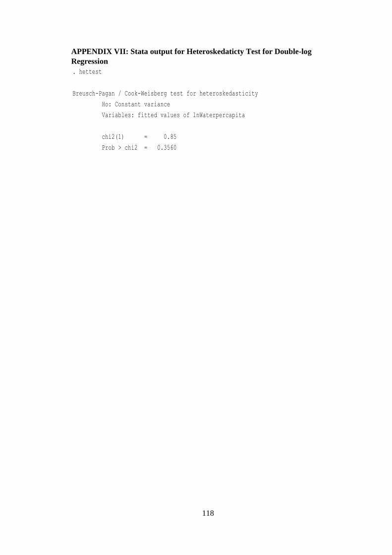
118

APPENDIX VII: Stata output for Heteroskedaticty Test for Double-log

Regression

Prob > chi2 = 0.3560

chi2(1) = 0.85

Variables: fitted values of lnWaterpercapita

Ho: Constant variance

Breusch-Pagan / Cook-Weisberg test for heteroskedasticity

. hettest