Household occupancy detection for burglary purposes
115
Household occupancy detection for burglary purposes Risk assessment and effectivity analysis of an unobtrusive, easy-to- implement countermeasure against Wi-Fi tracking. Tim Kers Master Thesis July 2018 Supervisors: dr. ir. P.T. De Boer dr. ir. M. Baratchi dr. ir. N Meratnia prof. dr. ir. G.J. Heijenk Design and Analysis of Communication systems (DACS) University of Twente P.O. Box 217 7500 AE Enschede The Netherlands Faculty of Electrical Engineering, Mathematics & Computer Science
Transcript of Household occupancy detection for burglary purposes

Household occupancy detection
for burglary purposes
Risk assessment and effectivity analysis of an unobtrusive, easy-to-implement countermeasure against
Wi-Fi tracking.
Tim Kers Master Thesis
July 2018
Supervisors:
dr. ir. P.T. De Boer
dr. ir. M. Baratchi
dr. ir. N Meratnia
prof. dr. ir. G.J. Heijenk
Design and Analysis of
Communication systems (DACS)
University of Twente
P.O. Box 217
7500 AE Enschede
The Netherlands
Faculty of Electrical Engineering,
Mathematics & Computer Science

I
Index
1. Abstract _____________________________________________________________________ 1
2. Introduction _________________________________________________________________ 2
3. Background __________________________________________________________________ 4
4. Research part 1: Joint occupancy detection study ___________________________________ 5
4.1. Introduction ______________________________________________________________ 5
4.2. Background ______________________________________________________________ 5
4.3. Method _________________________________________________________________ 7
4.4. Results _________________________________________________________________ 14
4.5. Problems and solutions ____________________________________________________ 29
4.6. Conclusion ______________________________________________________________ 31
4.7. Discussion ______________________________________________________________ 32
5. Research part 2: Conference setting _____________________________________________ 34
5.1. Introduction _____________________________________________________________ 34
5.2. Method ________________________________________________________________ 34
5.3. Results _________________________________________________________________ 35
5.4. Conclusions _____________________________________________________________ 45
6. Research part 3: Home scenarios ________________________________________________ 47
6.1. Introduction _____________________________________________________________ 47
6.2. Method ________________________________________________________________ 47
6.3. Potential influence of MAC randomization _____________________________________ 48
6.4. Automated vacancy detection on random households ___________________________ 57
6.5. Conclusions _____________________________________________________________ 62
7. Research part 4A: MAC randomisation implementations ____________________________ 64
7.1. Introduction _____________________________________________________________ 64
7.2. Problems with MAC switching in active networks _______________________________ 64
7.3. Implementation 1: Simple network re-authentication ____________________________ 68
7.4. Implementation 2: gratuitous ARP response ___________________________________ 68
7.5. Consideration ___________________________________________________________ 70
7.6. Other Factors and problems ________________________________________________ 70
7.7. Conclusion ______________________________________________________________ 74
8. Research part 4B: Variable transmission power implementation ______________________ 75
8.1. Introduction _____________________________________________________________ 75
8.2. Possible implementations __________________________________________________ 75

II
8.3. Limitations ______________________________________________________________ 76
8.4. Problems _______________________________________________________________ 76
8.5. Conclusion ______________________________________________________________ 77
9. Final conclusion______________________________________________________________ 79
9.1. Future work _____________________________________________________________ 80
10. References __________________________________________________________________ 81
11. List of figures ________________________________________________________________ 84
12. List of tables ________________________________________________________________ 86
13. List of algorithms ____________________________________________________________ 87
13.1. Chapter 5.3 ___________________________________________________________ 87
13.2. Chapter 6 _____________________________________________________________ 88
14. Appendix I: Documentation of the initial research __________________________________ 89
14.1. Informational letter _____________________________________________________ 90
14.2. Informational brochure __________________________________________________ 93
14.3. Blank timesheets _______________________________________________________ 98
15. Appendix II: Conference data error corrections ___________________________________ 101
15.1. Missing values ________________________________________________________ 101
15.2. Duplicate values ______________________________________________________ 102
15.3. Unrealisitic values _____________________________________________________ 102
15.4. SNR values of zero _____________________________________________________ 103
15.5. Conclusion ___________________________________________________________ 103
16. Appendix III, Household modeling and tracking ___________________________________ 104
16.1. Introduction __________________________________________________________ 104
16.2. Used data and limitations _______________________________________________ 104
16.3. Matlab household model: _______________________________________________ 110
16.4. Matlab data processors _________________________________________________ 110
16.5. References ___________________________________________________________ 111
17. Appendix IV: Report of prior literature research __________________________________ 112

1
1. Abstract Occupancy tracking by eavesdropping on household Wi-Fi networks is barely researched field with
the potential of being abused extensively. This risk was assessed by tracking the network in 55
participating households to find the potential of this type of eavesdropping. Due to various problems
in this experiment, most datasets were unusable. Definitive conclusions therefore couldn’t be drawn.
A countermeasure, not requiring networking protocol changes, was researched as well.
Unfortunately MAC randomization with variable transmission power proved to be ineffective in
preventing occupancy tracking in generated household network traces. Apart from theoretical
usability, implementation of MAC randomization proved difficult to implement without network
disruptions or serious changes to networking software. Practical use appeared limited as well as a lot
of other weak points remained. Current networking standards also lack feedback for proper
transmission power regulation requiring more additional software or creating more connectivity
problems. Also, information about the availability of fine-grained power control was lacking for
almost all common networking equipment.
Although the proposed solution proved inadequate in protecting households, the potential risk of
this type of eavesdropping should be explored further. For this, multiple improvements for future
research into the posed risk are listed.

2
2. Introduction Throughout the years, lots of research has been conducted around security flaws in wireless
networks and resulting tracking possibilities. For example: Tracking smartphones by their Wi-Fi
beacons proved to be an effective method to track traffic movements during rush hours and around
roadworks [1]. This can be used to improve road design to lighten congestion and pollution. On a
more controversial note, tracking people in and around shops allows for tailored offers and
advertisements [2]. And if we go further, we can find countless research on the possibilities of
tracking people in the public space and solutions to those possibilities. However, our most private
environment, the home environment, is researched a lot less.
Instead of the public space, a burglar could potentially use Wi-Fi tracking techniques to determine
vacancy in a household. While burglary rates are declining in the Netherlands, it still happens more
than 50 thousand times a year [3]. It is also a crime with a big and long lasting effect on victims [4].
The potential of this eavesdropping technique has been researched earlier on a small scale. This
small scale research showed more than 85% of occupancy predictions, determined by measured
network activity, to be correct in the tested households. The current research, discussed in this
thesis, is a continuation of that project, trying to prove the usability of this technique and to find a
countermeasure against it.
The main factor of the trackability of Wi-Fi enabled devices is the unique MAC address that each
device holds and broadcasts publicly, even when not connected to a network. To counteract the
same trackability in the public space, some smartphones apply MAC randomization while they are
unconnected to a network. But at home, connected to the network, these systems don’t work.
Removing or encrypting the MAC address potentially requires large changes to the network protocol,
leading to long adoption times and compatibility issues. A solution has to be found to prevent abuse
of the problem in the meantime.
Other researchers [5] have looked at the potential of MAC randomization while connected to large
public networks. The concept reduced trackability, but other factors like signal strength could
potentially reveal the connection between 2 addresses. Transmission power variations could be
enough to prevent this.
So when protocol changes are not desired, could mac address randomization with variable
transmission power be the easy to implement but effective countermeasure against Wi-Fi MAC
tracking in homes?
This research question is divided into multiple subquestions throughout this report.
Firstly, the potential threat is researched in chapter 3. A large scale experiment is conducted
with 2 other researchers after the example set in our earlier conducted research in this field
[6]. This research revolves around the subquestion: Is it possible to reliably track household
occupancy by Wi-Fi signals?
Secondly, the research conducted by Gruteser & Grunwald [4] is researched, repeated and
expanded with variable transmission power to answer the question: What research steps

3
were taken by Gruteser & Grunwald to prevent tracking in a conference setting and will
adding variable transmission power improve the effectiveness of their system?
Additionally, instead of a large public network, the technique is projected onto household
environments. Is a theoretical implementation of MAC randomization with variable
transmission power effective against occupancy detection in simulated household
environments?
Finally, the practical implementation is researched in separate chapters for mac
randomisation and transmission power adjustment. These chapters try to answer the
question: What possibilities are available, within currently used networking protocols, to
implement MAC randomization with variable transmission power?
Together, these main- and subquestions aim to expose the advantage of Wi-Fi eavesdropping on households from a burglar’s perspective and research a countermeasure that can be quickly implemented into existing networks before this abuse of this “weakness” becomes common.

4
3. Background The origins of this research lie in a small occupancy tracking experiment in a small number of
households [6]. This research showed that reliable occupancy tracking was quite simple with correct
prediction rate of 86.69% and only 2.82% false vacant predictions, which are the most problematic
for a burglar. The small number of data points and the usage of known participants make this
research statistically weak, but it does shown a possibility.
Although lots of research has been performed aimed at the possibility of WiFi tracking, it is usually
aimed at the public space [1] [7] [8]. Meanwhile, most households have a Wi-Fi network potentially
advertising the optimal burglary moments to anyone willing to listen. With the psychological effect
on the residents of a burgled home [4], not even mentioning the financial damage, this potential risk
should be tackled before burglars start abusing it.
The main weakness across a lot of these researches is the publicly visible MAC address of all
communicating devices [9]. The network layer holding this data is unencrypted and the addresses are
globally unique. Researched solutions like MAC spoofing and blind probe requests [7] may work in
the public space, but when authenticated in the home network it all falls away. Solutions aiming at
security improvements [10] try to solve spoofing and other possibilities by adding integrity checks to
the data, but still leave the problematic data publicly visible.
The most straightforward solution would therefore be to encrypt the MAC layer just like the layers
above it. This type of solution is also researched [11], but will require an overhaul of the 802.11
networking standards. This will take years to be implemented and even longer to be common.
Meanwhile, people just have to hope that no burglar uncovers this possibility.
In parallel, three researches are conducted into different solutions for the same problem. One
research focusses on the development of an auxiliary device mimicking the users network patterns to
scramble the actual occupancy. This solution is visioned as an off-the-shelf solution people can
simply buy for their home.
At the other end of the scale, another researcher looks into the implementation of MAC layer
encryption within the current networking standard. This solution is quite optimal, but potentially
hard to implement into existing networks therefore having a long adoption time
This research lies between the other two and tries to find an intermediary solution to protect
households and their residents while we wait for the implementation of a more optimal and
permanent solution. The goal is therefore an easy to implement solution, ideally only requiring a
software update to a client device.
Additionally, with the three researchers combined, the small scale tracking experiment is repeated
on a larger scale with a randomized test set. The goal for this part is to definitively proof the potential
of WiFi tracking for a burglar and indicate the importance of countermeasures.

5
4. Research part 1: Joint occupancy detection study
4.1. Introduction This chapter covers the research into trackability of household occupancy using the Wi-Fi network.
This research is a follow-up of an earlier small-scale research (see appendix 1) performed by the
same researchers among the households of relatives. The usability of that research was very limited
due to the scale and potential bias. This research tries to prove the potential of Wi-Fi eavesdropping
to track occupancy in households.
The execution of this research is a joint effort between [name] [name] and [name]. These
researchers performed their own research into potential solutions against Wi-Fi tracking. This
chapter, assessing the potential risk of eavesdropping on Wi-Fi networks is a joint effort between
[name] and [name] and will be identical between their respective theses.
The research is divided into 2 parts. Due to practical reasons, the measurements are conducted in
the living quarters on the campus of the University of Twente. These living quarters feature a shared
Wi-Fi network called Eduroam. Instead of separating the devices per household by their used
network, as would be possible in normal households, this shared network throws all devices on one
pile. Or at least from the burglar’s perspective.
The first research step, would be to use other parameters to determine the critical devices for the
participating household. After this step, the situation is again similar to normal households where
only relevant devices are registered. At this point, the trackability of the network can be determined.
This chapter therefore knows two research questions:
Is it possible to determine which Wi-Fi devices belong to a certain household in a shared
network with only passively detectable parameters?
Is it possible to reliably track occupancy in a household with passive eavesdropping on its Wi-
Fi traffic?
4.2. Background As stated in the introduction, this research was preceded by a small-scale experiment in 2016. In this
small-scale research, borrowed laptops were used as measurement devices which limited the group
of participants to relatives and friends. Unfortunately, the stability of the borrowed hardware and
the many configuration onto which the software had to work proved to be a problem. Combining this
with a very limited timeframe, limited the experiment to 12 households. Which in turn limited the
statistical relevance of the research.
The results, however, did indicate a potential problem with household Wi-Fi networks. On average,
86.7% of predictions were correct. The 13.3% faulty predictions were made up of false occupied
(10.5%) and false vacant predictions (2.8%). For a burglar, false occupied predictions are potentially
missed opportunities. However, as long as other opportunities are available, this is not really a
problem. The false vacant predictions are problematic for a burglar. These are the times they would
think the house was vacant while it was not and would risk getting caught.

6
Most of these false vacant predictions occurred at night, partly due to households having limited Wi-
Fi coverage in the bedrooms causing residents to turn their Wi-Fi off at night. When the 00:00 to
07:00 timeslot was removed from the analysis, correct ratings increased to 89.3%, false occupied
declined to 10% and false vacant diminished to 0.7%.
Although less relevant to this research, a small social study was conducted as well. It showed that
participants felt slightly less safe in their neighbourhood, with safety grade lowering from 7.5 before
and 7.33 after the research, on a scale of 10. More people had the feeling of being unsafe in their
homes (50% before to 58.33% after) and the likeliness of a burglary happening to them in the next 12
months was graded 1.6% higher than the 25% before the research.
The social part of the previous research was not included in the new research. This was mainly due to
the amount of time and effort it involved to get all participants to fill in the forms. The forms also
required more work from participants, which was deemed as a potential deal breaker for them.
Additionally, this research focuses on the technical side of this potential problem. The social study is
not regarded as relevant for this part.
Unlike previous research, this one was intended to prove the potential of eavesdropping on
household networks in a statistical relevant matter. This required larger datasets and a non-biased
group of participants. The latter is tackled by randomly choosing households out of a list of living
quarters on the campus of the University of Twente. This is further explained in paragraph 4.3.1.1.
This yielded a list of 556 potential participating households. We estimate that a quarter of the
potential participants will be willing to participate. To retain a level of randomness in the selection of
the participants, we will use a maximum of 50% of this list. This leaves an upper limit of around 70
participants.
For statistical experiments the required number of samples can be determined by [12]:
𝑛 = (𝑍𝜎
𝐸)2
Where, Z is dependent on the confidence level. In this case, 95% yields a Z of 1.96. 𝜎 indicates the
standard deviation, which is fairly unknown at this point and therefore set to 50%. E is the margin of
error which is plotted against the sample size (n) in Figure 1 below

7
Figure 1: Confidence level vs sample size for the university campus household list
To reach sub-10% intervals, sample sizes of 100 and higher are required, which is not feasible with
our pool of participants. Therefore, a compromise was made to aim for a 15% or better confidence
interval and the accompanying requirement of 43 or more datasets. This was deemed feasible with
the available time and equipment and keeping in mind some problems on the way.
4.3. Method This experiment is split into three parts. First, measurement equipment is placed in the homes of
participants to gather network traces to be used in the later parts. The residents receive a form on
which they are asked to keep their presence to be compared with the retrieved data afterwards.
After retrieval, the filled-in timesheet and trace data are pre-processed to prepare for the next parts.
In the second part, the pre-processed data is processed to remove any device not belonging to that
household.
The third part would then aim at extracting an occupancy schedule from the network trace and
compare this to the schedule filled in by the participant.
4.3.1. Part 1: gathering network traces from households
In the original experiment, datasets of multiple weeks were recorded to try and recognize recurring
patterns in people’s lives. In this research, the datasets are chosen to be only one week to try and
reach a higher number of datasets in the available time frame for this research. The focus therefore
lies on reliable occupancy detection instead of pattern recognition. When occupancy detection can
be performed reliably, pattern detection should not be a problem.
As the research potentially involved privacy sensitive data of the occupants, the research proposal
was reviewed by the Ethical board of the EEMCS faculty at the University of Twente. This gave some
restrictions on target groups and data storage that will be explained further down in this chapter.
0
5
10
15
20
0 25 50 75 100 125 150 175 200 225 250 275 300 325 350 375 400
Co
nfi
de
nce
inte
rval
(%
)
Sample size

8
4.3.1.1. Target group
A problem with the earlier experiment was the use of relatives as test subjects, this gave potentially
biased data and therefore should be avoided in the new experiment. For this new experiment,
subjects should be chosen at random from a large pool of potential candidates.
The ethical board gave an important restriction on the potential candidates. All occupants in a
participating household must be able to understand and consent to the potential privacy risk. This
prohibits measuring households with for example underage children or mentally challenged people.
Eventually the aim was set on student housing. This gives an easily containable set of candidates,
almost no underage people and very small chances of children living in and/or visiting the household.
This left two possible groups: Dormitories and individual living quarters. Dormitories posed a couple
of potential problems.
When measuring a complete dormitory, all students living there must consent. With living
groups up to 16 people, it is not unlikely that at least one would refuse.
Standard measurement equipment would probably lack the range to cover the complete
dormitory, thus requiring more equipment and opening the door for synchronisation issues
and/or potential blind spots.
Alternatively, measurements could focus on individual occupants in a dormitory. A measurement
device could then be placed in the room of the participating student. However, this gives a similar
range problem. When a student leaves his room to eat in the shared living room, he or she is likely to
be out of range. This system would consider this as “absent”. The student should therefore note his
presence in the actual room, which quickly becomes a hassle and error prone.
Ultimately, the choice fell on individual living quarters on the university campus. The housing agency
provided us with a list of 556 individual housing quarters found across campus. These are divided in
full apartments, studios and standard sized rooms with personal facilities. These areas are all
coverable with standard Wi-Fi products and are usually occupied by one or two people.
4.3.1.2. Privacy considerations
As this research involves privacy sensitive information about people and their household, some
precautions had to be taken:
No user data is stored by the measurement device at all
The device identifier (the MAC address) is only stored as a hash to stop anyone from finding
easily finding the original device. Although scanning the whole campus could still be easily
done, preventing such action is fairly hard whilst keeping usable data. Additionally, anyone
with such interest would be better suited with gathering newer data instead of trying to
crack the old.
The retrieved timetable is linked to the measurement device its device number. However,
this number is never linked to a house address, phone number or email address. This means
that there is no way to link a dataset or timetable back to a household or individual.
After retrieving the measurement device, all data is removed from the SD-card before
reusing it for another household. Although the stored data would be barely usable for any
adversary, this prevents other people from retrieving the data.

9
All research data is to be permanently removed no later than 1 year after completing the
research, as stated in the original research proposal (see appendix 1). The data is only
accessible to the researchers and supervisors stated in the proposal and brochure.
4.3.1.3. Measurement equipment
For these measurements a device was required to capture network traffic. As student housing is
covered with the Eduroam Wi-Fi network, monitoring this network is sufficient in most cases. The
network is divided over the three Wi-Fi super channels (channel 1, 6 and 11) thus requiring 3
network interfaces. The choice fell on the Orange pi lite minicomputer. This creditcard sized
computer features an onboard Wi-Fi module (XR819) and two additional USB ports for two additional
USB Wi-Fi card (Ralink RT5370).
An important parameter was the support for monitoring mode on the Wi-Fi interface. This was a
problem with selecting a Raspberry pi. Its on-board module does not support monitoring mode
requiring us to add 3 external Wi-Fi modules. Furthermore, the cost of a raspberry pi is almost
double that of the Orange pi Lite.
For the OS (Ubuntu) and measurement data, a 16GB micro SD card is used. With data compression
used in our system, this would easily cover measurement data for multiple weeks.
Figure 2: Measurement equipment
10
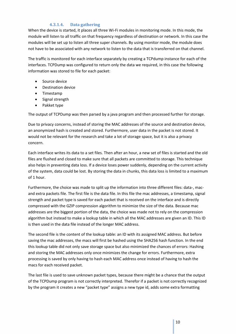
4.3.1.4. Data gathering
When the device is started, it places all three Wi-Fi modules in monitoring mode. In this mode, the
module will listen to all traffic on that frequency regardless of destination or network. In this case the
modules will be set up to listen all three super channels. By using monitor mode, the module does
not have to be associated with any network to listen to the data that is transferred on that channel.
The traffic is monitored for each interface separately by creating a TCPdump instance for each of the
interfaces. TCPDump was configured to return only the data we required, in this case the following
information was stored to file for each packet:
Source device
Destination device
Timestamp
Signal strength
Pakket type
The output of TCPDump was then parsed by a java program and then processed further for storage.
Due to privacy concerns, instead of storing the MAC addresses of the source and destination device,
an anonymized hash is created and stored. Furthermore, user data in the packet is not stored. It
would not be relevant for the research and take a lot of storage space, but it is also a privacy
concern.
Each interface writes its data to a set files. Then after an hour, a new set of files is started and the old
files are flushed and closed to make sure that all packets are committed to storage. This technique
also helps in preventing data loss. If a device loses power suddenly, depending on the current activity
of the system, data could be lost. By storing the data in chunks, this data loss is limited to a maximum
of 1 hour.
Furthermore, the choice was made to split up the information into three different files: data-, mac-
and extra packets file. The first file is the data file. In this file the mac addresses, a timestamp, signal
strength and packet type is saved for each packet that is received on the interface and is directly
compressed with the GZIP compression algorithm to minimize the size of the data. Because mac
addresses are the biggest portion of the data, the choice was made not to rely on the compression
algorithm but instead to make a lookup table in which all the MAC addresses are given an ID. This ID
is then used in the data file instead of the longer MAC address.
The second file is the content of the lookup table: an ID with its assigned MAC address. But before
saving the mac addresses, the macs will first be hashed using the SHA256 hash function. In the end
this lookup table did not only save storage space but also minimized the chances of errors: Hashing
and storing the MAC addresses only once minimizes the change for errors. Furthermore, extra
processing is saved by only having to hash each MAC address once instead of having to hash the
macs for each received packet.
The last file is used to save unknown packet types, because there might be a chance that the output
of the TCPDump program is not correctly interpreted. Therefor if a packet is not correctly recognized
by the program it creates a new “packet type” assigns a new type id, adds some extra formatting

11
information and saves this to this file. If this packet type is encountered again it could use the
information saved with the previous packet to identify it as the same type.
4.3.1.5. Measurement procedure
From the original list of households, a random selection of 60 households at a time is chosen by a
Matlab script using the standard rand() function with a random seed of 42. These households receive
an introductory letter about the research to give them some time to consider participating. Then,
after approximately a week, the houses are visited and the residents asked if they would like to
participate in the research. If required, additional information can be given. If nobody is home at that
time or the participant wishes some extra time to consider participating, the household is tried again
at a later time. Obviously, a resident is free to decline participation without reasoning, after which
the house is removed from the list.
When a resident chooses to participate, one of the measurement devices is handed over and plugged
into a power socket inside the house. Additionally, the subjects get a form with a timetable on which
they are asked to keep their presence log during the measurements. This timetable is used as a
reference to validate the conclusions drawn from the measurement data. For extra information
about the research, the privacy concerns and proper actions, should they want to stop the
measurements, an informational brochure is handed over for them to keep. Finally, the participant is
asked for contact information such as a phone number or email address so that, after a week of
measuring, the participant can be contacted for retrieval of the device and timetable.
The introductory letter, blank timesheet and informational brochure are added in appendix I of this
report.
4.3.1.6. Initial data processing
After retrieval of the measurement device and timetable, their data has to be processed before it can
be used to identify occupancy.
Timesheet processing
All timesheets are scanned and digitally processed. Initially, the “marked” fields are made uniformly
black to prevent reading error by the automated processor. An example of this is shown in Figure 3.
Figure 3: Example of a timesheet day before and after initial processing
After this step, the images are loaded into an automated processor, created in Matlab. This program
lines up the filled in timesheet with a reference (empty) version and determines the light level of
each data field (white or black, indicating unmarked or marked). For this, predetermined coordinates
are used, derived from the reference timesheet.

12
Participants were allowed to choose if they preferred to mark for “absent” or “present” as long as
they indicated their choice on the timesheet. Additionally, participants sometimes mixed up days or
started marking at a different day than the first one on the form. All these factors were manually
entered into the processor, which (where applicable) inverted the derived schedule or rearranged
the days.
The result of each timetable is a text file with 7 lines (days) of 96 characters (quarters). For each
character, a ‘0’ symbolizes vacancy and a ‘1’ occupancy.
Trace data processing
As discussed in saving data part, the device saves three files per interface per hour. The choice was
made to do some pre-processing on this data to lower the amount of data that had to be processed
every time. To do this a program was written that would read and uncompress this data and
summarize the presence for each device. This was done by creating blocks of 5 minutes in which
packet type count, the minimum, maximum, average signal strength and to whom each client was
talking to was saved. This data was then exported to a csv file to allow further processing in Matlab.
4.3.2. Part 2: Automated filtering of relevant devices
4.3.2.1. Selecting devices within the household
In a normal household environment, a burglar can select a certain network and therefore household
to track. This allows him to only track devices using that network. Unfortunately, just as many
universities, the University of Twente uses the Eduroam network across the entire campus including
the living quarters. As a lot of students will be using this, the distinction between houses disappears.
This means that other steps have to be taken to extract devices belonging to the targeted household.
If this step succeeds, the remaining trace only contains legitimate devices for that household and the
situation is again similar to a normal household.
Two factors were used to determine devices belonging to that household. The measurement device
logged the signal-to-noise ratio of every received device throughout the week. With the device
placed within the household, the devices with the highest ratings will most likely belong to that
household.
As a second factor, the interaction between different devices is checked. The idea behind this is that
devices within the same household may often communicate with each other. For example, a laptop
checking the availability of a network printer, or a mobile phone streaming a video to a smart tv.
With this second step, a device tucked away in a corner or cupboard but belonging to that household
may still be recognized while its SNR values would imply it is a device from another household.

13
4.3.2.2. Selecting devices with usable characteristics
Nowadays, many different devices can be present in networks. A burglar will probably be best served
with smartphone availability, as this device is mostly carried around with the residents. Laptops,
tablets and other devices could give similar information.
But a stationary device like a network printer, being active all day long, would not be very interesting
to determine occupancy. Therefore, some extra filters are added to separate usable devices from the
trace.
Discard devices with high active or inactive rates
A device that is communicating continuously or barely does not give much insight in any
resident’s schedule. Therefore, any device that is active for more than 95% of the time or less
than 5% of the time is discarded. The likelihood of a resident having such a schedule is
almost zero.
Session lengths
Schedules differ between people, but some factors are fairly constant. Over the period of a
week, one can expect the residents to be home for some lengths. For example, because they
sleep at home. Therefore, a filter is created that looks at the occurrence of certain session
lengths. For example, if a device is never present for a couple of hours, it is very unlikely that
its trace will represent the residents schedule
Session counts
Similar to session lengths, session counts can be used as a parameter as well. A real person
would not come home and leave every 10 minutes (for example), nor would they stay at
home for 5 days and then disappear for the weekend. In the first situation, it is more likely
that it involves a device connecting periodically. In the latter, it looks more like a stationary
device, but it is turned off when the resident leaves for the weekend. Although exact
boundaries for “legitimate” devices are hard to draw, the extreme situations as stated above
can be removed relatively safe.
4.3.3. Part 3: Extract household occupancy from network trace data
In a normal household, the Wi-Fi network would be used by the people and devices belonging to it.
This makes tracking much easier as the trace would not be influenced by neighbouring devices. In the
chosen Eduroam environment, all households share the same network. But after extracting the
appropriate device traces from the dataset, the situation should again be comparable to a normal
household.
The next step is to generate occupancy schedules from the network trace and compare this to the
schedules filled in by the participants. A burglar will aim to minimize risk. As he will need only one
free moment, it is less relevant if other potential moments go unnoticed due to an overly safe
technique.
The safest options to start with is to regard every captured device as relevant. Only when all devices
become silent, the house is regarded empty. In addition to that, a burglar would not be interested in
free windows of a couple of minutes. Instead, only continuous vacancies of 15 minutes or more are
deemed relevant.

14
As with all of these predictions, the burglar would be looking for an absolute minimum false vacant
predictions. These are the moments he could be detected. As long as not all potential moments are
lost, no technique is “too safe”.
4.4. Results
4.4.1. Part 1: gathering network traces from households
Gathering the network traces from the households proved to be a very time-consuming process.
Apart from all the hours distributing introductory letters, asking for participation and retrieving
devices, a lot of time was consumed by software issues on the measurement devices and to process
the data.
4.4.1.1. Start-up phase:
Before being able to distribute any device, software had to be created for the measurement
equipment. In this step, multiple test rounds were conducted to test the software for functionality
and reliability. Some problems were found and resolved in this phase, like occasional failure to
initialize a network interface. In these cases, one of the interfaces became unusable for the data
logging software. As this problem was detectable and re-initialization of the module was sufficient,
this problem was effectively resolved.
4.4.1.2. First measurement round:
After multiple rounds of short and long tests, the system was deemed ready for deployment.
Unfortunately, after the first round of real-world tests, the resulting data from all 10 participating
households came back corrupted. The cause of this was found to lie within the LZMA compression
algorithm used to compress the recorded data.
The problem turned out to be a memory allocation issue and finding a solution within the
compression software proved difficult. Fortunately, storage space turned out to be plenty for a week
of data allowing a switch to the more commonly used but less efficient Gzip compression algorithm.
This solution was tested in multiple networks for multiple days and proved reliable.
4.4.1.3. Final measurement rounds:
After the problem in the first round of measurement was resolved, multiple successful measurement
rounds were performed before the holidays put a stop to this research step. In total, 45 households
participated in these rounds before the holidays brought a stop to them.
Of these 45, 8 were lost due to administrative mistakes. 6 of them were found to be checked off, but
never actually retrieved. Due to the long period between data gathering and processing, this
discrepancy went unnoticed. The participants were contacted when this problem was found. The
device was successfully retrieved from two residents. one admitted the device was never retrieved,
but lost it while moving to a new house. The other three never responded.
15
Two other devices remain unaccounted for. It could be that they are also still out there with
participants, but we were not able to find out who. The strict separation between consent forms
(with personal information) and devices and their data may be good for privacy concerns, but did
prevent us from backtracking which consent forms were never met with data.
On top of the administrative error, one dataset became unusable as its accompanying timesheets
went missing. With that, only 36 datasets remained before processing even began.
Although the major issues were resolved, some measurements still developed problems. Some of the
found problems were:
Measurement devices missing data from one of the network interfaces. This looks similar to
the earlier initialization error, except that the software never found an initialization error nor
were there any problems reported in the system’s logs. Normally, a problem with one of the
network interfaces should trigger a system reboot to try and re-initialize everything.
However, this did not happen and the system continued its operation with two interfaces.
This problem only occurred in one of the measurements making a not completely plugged in
USB Wi-Fi modules plausible.
Measurement devices seized to record any data during the measurement period. Although
the device was placed for a minimum of 7 days, the trace would only cover a couple of hours
or days in some cases. Similar to the previous problem, no evidence of it was to be found in
the systems logs. A possible cause could be a loss of power. Maybe a resident moved the
device causing the power jack to become loose or unplugged an extension cord while
forgetting the device that was placed there. In total, 5 devices showed these kinds of
problems with their active time varying between 26 and 95 hours. One of these devices had
its data split with a reboot in between. As the device does not have a real time clock, there is
no data on the amount of downtime between these two sessions.
Measurement devices developing corrupted files within the data. This could have been
caused by a power loss or other reboot event. This problem affected two devices, but only
influenced a couple of files. The software was created to store data in one-hour blocks to
prevent large data loss in such cases. Therefore, the datasets remained usable, although
missing an hour somewhere.
Devices not logging any data. In total, three devices came back without any measurement. In
one of the cases, this was due to the SD card not being inserted properly. Although powered
all week, the device never measured or even booted. The second device did boot up and
created the initial logging files and system log entries, but the device probably stopped
working soon after that. No further logging files were created (which should have happened
every hour) and system logs did not show any more data. The last device had its power jack
not inserted properly due to the improvised (cardboard box) case used for 10 devices.
Eventually, the holidays limited the available time for measurements as a large amount of the
residents moved away for some time. In the end, after removing all faulty datasets, only 25 datasets
remained to be processed further. Unfortunately, this is far less than the aimed minimum of 43,
limiting the statistical relevance of the outcome of this research. The confidence interval was now
limited to 19.2%, assuming no further problems arose.

16
4.4.2. Part 2: Automated filtering of relevant devices
Due to the choice of an area with a single large Wi-Fi network, it was expected that neighbouring
devices would be picked up in the measurement. The first step would be to remove these from the
trace. The resulting dataset should ideally only include all devices belonging to the participating
household. This situation would be similar to a measurement in a normal household where devices
are separated by their used network.
4.4.2.1. Original approach
While processing the data, the number of unique devices recorded in the measurements proved to
be extremely high. As the experiment was conducted in the Eduroam environment, it was expected
that large amounts of devices would be found from neighbouring households. However, it was not
expected that most datasets would contain hundreds of recorded devices and some which even
went up to hundreds of thousands.
One cause for this huge number of devices is people passing by the house. This would result in a
registration of their device (if active on Wi-Fi) for a short amount of time. Additionally, the MAC
randomization scheme of some versions of IOS and Android would create a lot of “fake” devices as
long as the devices has its Wi-Fi capabilities enabled but is not connected to a network.
Multiple rounds of filtering were used to try and remove any unwanted device from the traces.
Initially, 5 datasets were picked as training set to adjust the filters. These filters would then be
applied to the other datasets.
Remove extremely short and long presences
People walking by or devices with MAC randomization create a lot of data that is not usable for
occupancy tracking. Therefore, all devices that were picked up for a total of less than 5% of the total
measurement duration, or approximately 8 hours out of the week, were removed from the trace.
This includes MAC randomizing devices, people walking by and someone visiting during the week.
Additionally, devices that were present for more than 95% of the time were also removed. These
devices include access points and stationary devices. These devices yield no information about the
resident’s presence and are therefore fairly useless for a burglar.
This filter removed a major part of “unusable” devices from the trace and reduced the datasets
mostly to sizes between 25 and 75 devices.
Group devices together by mutual communication
The idea behind this filter was that devices belonging to the same household are more likely to
communicate with each other. For example, video streaming from a laptop to a TV, or sending a
document to a network printer.
Unfortunately, devices proved to be much more talkative than that. Intercommunication happened
everywhere in the dataset making distinction between different device “groups” impossible.
Therefore, this filter was not used any more.
Remove devices with low signal strength
Devices within the household are in close proximity of the measurement device and should therefore
read high SNR values. Finding the exact threshold after which a device does not belong to that house

17
is going to be difficult due to all the different circumstances in and around the households. However,
it can be used to filter out “distant” devices and reduce the dataset by a significant amount.
Figure 4 shows the signal strength distributions in one of the datasets gathered in this experiment.
Most devices reside in the far left of the graph, making them most likely to be distant. However, it is
difficult to select proper thresholds to distinguish devices actually belonging to the household.
Manually comparing the dataset to the filled-in schedule revealed 1 perfectly matching device.
However, when looking at the average signal strengths, that device came second with the first device
showing no relation to the schedule. When looking at peak values, the matched device fell down to
16th place.
Figure 4: Signal strength distribution of the measured devices in 1 household
No similarity in the results was found across the datasets. The original training set of 4 datasets was
even doubled to 8, to try and find the best matching filter settings. However, the filter was not able
to remove all “unwanted” devices without losing genuine ones as well.
Another problem that arose, was the lack of “matching” devices in a lot of datasets. Although some
devices showed high signal strengths, they would not be comparable to the schedule that the
resident filled in. This problem is further worked out in 4.4.3: Alternative approach.
Session lengths
Analysis of the datasets showed some interesting characteristics in some devices. For example, some
devices would show enormous amounts of activity, but all in short bursts.
Although it is unclear what kind of devices these actually are, but it is not likely to reflect the
schedule of a resident. An actual resident would normally have periods of presence and absence. To
try and filter for those characteristics, session lengths were checked. It would be likely that a resident
would have multiple presences of a couple of hours during the week, for example to sleep, study or
relax.
This filter proved reasonably effective. Many devices with the behaviour talked about above were
filtered out. Specific filter settings proved to be only mildly influential. Any setting for a couple of

18
presences of a couple of hours was reasonably effective. The filter was only effective in removing
unusual devices, not in selecting devices for a specific household.
Session counts
This filter had a similar aim to the previous one. During a week, a resident would probably leave a
number of times. But to the rapid transitioning devices mentioned earlier showed extremely high
numbers. Other stationary devices that had 1 period of absence would pass through the <95% filter,
but would show very low session counts.
This filter was set out to filter out unrealistic low and high session count numbers. Although
reasonably effective, it did not have any influence over the session length filter. Therefore, this filter
was eventually dropped.
4.4.2.2. End result
In the end, a uniformly applicable filter was not achieved. The filters, when combined, gave a
reasonable decline in device count, but returned both genuine and neighbouring devices. Even within
the test group, with prior knowledge of the schedules, no acceptable result was achieved.
As mentioned earlier, many datasets appeared to be lacking “genuine” devices at all, when
comparing to the residents’ schedules. Of the original 4 datasets selected as a training set, only one
showed clearly matching devices and one other showed similar (but not perfectly matching) devices.
This raised the question if it was even possible to extract occupancy information from these datasets.
Therefore, the original filtering approach was halted, and the focus now came on verifying if there
was actually usable data in the datasets before continuing.

19
4.4.3. Alternative approach
As mentioned before, a lot of datasets appeared to be lacking any devices matching to the schedule.
This raised the question if occupancy tracking was even possible with the devices picked up by the
measurement devices.
Therefore, instead of using a training set, all datasets were manually compared to the schedules to
find any (seemingly) matching devices. Although time consuming, the easiest method proved to be to
plot (a subset of) the devices together with the schedule and visually match them together.
Automated versions were tried, but they would occasionally miss devices or incorrectly match them.
Sorting the devices by their mean signal strength proved to be effective. The matching devices would
(as expected) usually occur in the top part of the selection. In the end, potentially matching devices
were identified in only 14 of the remaining 25 datasets. In most households one of the identified
devices would closely matching a device. Any other would have a lot of resemblance, but also errors.
Figure 5 shows a comparison between two visually matched devices and the accompanying
schematic.
Figure 5: Detected presence of two visually matched devices against the user’s schedule
Both devices behave similar to the schedule. However, the bottom device often becomes
intermittent when the user is supposed to be away. This is likely to be the behaviour of a stationary
device periodically checking the return of known devices. The real “user” schedule appears to be the
middle graph.
To get an impression of reliability between the schedule and trace data, the visually best matching
device of each household was selected and scored. These devices are likely to be smartphones and
similar devices, closely representing the user’s presence. These results are presented in Table 1
below.
Correct occupied prediction Correct vacant predictions Total correct predictions
90.4 % ± 8.9% 87.6% ± 11.9% 87.8% ± 9.8%
Table 1: User presence results with their respective standard deviations

20
This result does indicate that occupancy could be determined from Wi-Fi data, if the correct devices
can be selected from the dataset. However, this result only covers 14 datasets out of 25.
4.4.4. Part 3: Extract household occupancy from network trace data
As explained in part 2, the automatic filtering of devices proved problematic. The proposed method
of only selecting relevant devices with filters and extract occupancy out of that is therefore difficult.
Instead, this part is split into 2 parts. First, all visually matched devices of the household are
combined and scored. These devices are the most likely to reside within the same household. This
combined dataset is compared against the user’s schedule to see if usable data has remained.
Additionally, some of the filters of part 2 are reused. Although the filters were not able to remove all
“wrong” devices, they may still be usable. If genuine devices are present in the dataset, combining
them with “wrong” devices only removes potential vacant moments. But it does not add false vacant
readings.
Unfortunately, this technique is only applicable to the datasets in which at least one device was
recognized. As the measuring equipment lacked any means of measuring date and time, there is no
way of lining up the measurements with the schedule without visual checks. A rough estimate can be
made, but the manually checked datasets showed various amount of offset remaining.
4.4.4.1. Combining visually matched devices
This technique was only applicable to 7 of 14 the households with visually matched devices. In the
other 7, only one device was matched to the schedule. The single device matches were already
covered in part 2. The remaining datasets had two (4 times), three (twice) or five (once) devices
matched to their schedules.
For each dataset, the traces of all devices are combined into one. Combining the devices effectively
performed an “OR” operation on the traces. If any of the devices is present at that moment, the
combined trace is too. From a burglar’s point of view, this is the safest option. Only when no device is
active, the house is regarded empty. The combined trace is added to the first figure presented for
each dataset, this to give an overview of the used data.
Afterwards, short absences are removed from the combined trace as a burglar would not be
interested in those. In the second graph, three versions of this filtered combined trace are then
presented with different minimum absence settings.

21
4.4.4.2. Dataset 1
In the first dataset, 2 devices were recognized. Figure 6 shows their behaviour compared to the
schedule. The 2 devices share a number of absences which in turn match roughly with the schedule.
However, there is a slight offset between the absences in the schedule and the devices at some
times. This could be down to small errors when filling in the schedule.
Figure 6: Dataset 1, comparison between network traces and user's schedule

22
As a burglar would not be looking for absences of mere minutes, some additional filtering was
required. Figure 7 shows the original schedule and the combined trace, filtered for absences of more
than 15, 30 and 60 minutes.
Figure 7: Dataset 1, comparison between the user's schedule and measured absences
At this point, it is a bit problematic to decide which offset between measurements and schedules can
be regarded as still valid. For example, the absence at 72 hours is measured slightly later than the
schedule states, but there is a reasonable overlap. Completely at the right of the graph, the
measured absence is shifted free of the schedule. They are reasonably similar in length and a
schedule error is not unlikely, but there is no definitive answer. At the other hand, the measured
absence at approximately 33 hours is shifted a lot more from the long-scheduled absence starting at
24h. Additionally, the duration is completely different as well.
These uncertainties make it impossible to capture the result in numbers, but they do give an
impression. In this dataset, the longest measured absence (just before the 48h mark) matches
perfectly with the schedule. Should the burglar’s measurements have returned this data, picking the
longest absence would have been “safe”.
4.4.4.3. Dataset 2
The second dataset yielded 5 potentially matching devices although none of them prove to be a
perfect match. The schedule did not give much room for comparison as it only showed two absences.
It is not unlikely that the resident forgot to register some (maybe shorter) absences.
However, Figure 8 shows that combining these devices still give useful information. The long absence
from the schedule largely returns in the combined trace. The smaller absence in the combined trace
also matches with the large vacant slot of the schedule, giving this prediction an almost perfect
score.

23
Figure 8: Dataset 2, comparison between network traces and the user's schedule
Filtering on absence length does not make a difference in this dataset. The small absence in the
combined trace is still an hour long. The 3 filtered traces (15, 30 and 60 minutes) therefore yield
exactly the same graph.
4.4.4.4. Dataset 3
Dataset 1 showed some “unstable” presence like a stationary device could create. In that dataset, it
did not prove to be a large problem. This dataset however, has a device that influences the combined
trace a lot.
Figure 9 shows the two devices recognized for this trace. One of which displays periodic activity
when de resident is away from home.
Figure 9: Dataset 3, comparison between network traces and the user's schedule
When filtering this combined trace for periods of 15, 30 and 60 minutes, only a couple of options
remain with a maximum length of just over an hour. Meanwhile, the schedule shows plenty of
opportunities.

24
Figure 10: Dataset 3, comparison between the user's schedule and measured absences Fortunately, for a burglar, the stationary device is recognized easily. Additional filtering or manual
adjustments could still reveal the real absences which device 1 clearly shows.
4.4.4.5. Dataset 4
Also, with 3 recognized devices, dataset 4 also shows some “unstable” behaviour, especially in device
1. However, the influence is a lot smaller. Figure 11 shows that the large absences are still
recognized, although the largest absence is divided in multiple pieces.
Figure 11: Dataset 4, comparison between network traces and the user's schedule
Filtering with 15, 30 and 60 minute thresholds barely influences the combined trace apart from
removing some of the fast switching. However, a burglar would have already chosen the large
absence.

25
4.4.4.6. Dataset 5
In this dataset, two devices were found to be matching the schedule. However strangely, both traces
were virtually identical to each other and the schedule. The combined trace of Figure 12 therefore
needs no further filtering. The data already matches the schedule without any mistakes.
Figure 12: Dataset 5, comparison between network traces and the user's schedule
4.4.4.7. Dataset 6
Similar to dataset 5, both devices in this dataset are similar to the schedule. The combined trace
therefore matches very well. However, Figure 13 shows the potential risk of using this kind of
presence tracking. The schedule states that the resident was home at approximately the 130-hour
mark, but both devices were silent. This would be a risk, should the burglar decide to abuse that
“absence”.
Figure 13: Dataset 6, comparison between network traces and the user's schedule

26
4.4.4.8. Dataset 7
The last dataset had 3 matching devices as shown in Figure 14.
Figure 14: Dataset 7, comparison between network traces and the user's schedule
Device 2 introduces some “unstable” behaviour, but this time it prevents false vacant predictions at
approximately 12 and 40 hours. The remaining absences all match with the schedule, especially the
main absence of a couple of days.
4.4.4.9. Combining top SNR devices
The usability of the previous results is severely limited. It only shows that device data could be used
to determine occupancy. But to be able to do that, a burglar still has to extract the right devices from
the full dataset without the prior knowledge of the schedule. When operating in a normal house
network, the network itself will only be used by residents and maybe visitors removing this problem.
Unfortunately, reliably extracting the appropriate devices from the large Eduroam dataset has
proved impossible. This prevents us from proving that these techniques are reliable.
However, some use may still be present in the dataset. As stated earlier, a burglar is only interested
in one opportunity, as long as it is reliable. Maybe, the filters were not perfect, but still good enough.
To test this, the dataset is initially sorted by signal strength. Afterwards, the first device is taken and
compared to the schedule, then the first 2 devices are taken together and compared and so on. The
manually recognized devices mostly resided in the top part of the dataset when sorted by signal
strength.
All these combinations produce a certain relation between the correct and false vacancy predictions.
This relation, with the imperfections of “wrong” devices, may still be able to deliver usable data for a
burglar. Figure 15 shows these combinations and their average false vacant and correct vacant scores
as a part of the total vacancy displayed by the schedule.

27
Figure 15: Average false and correct vacancy prediction rate versus device count
The graph clearly shows that the false vacant occurrences decline as the number of devices increase,
but so do the correct vacant occurrences. Instead of getting a sweet spot where the false vacant
predictions become negligible and true vacant predictions still occur often, both factors follow
reasonably similar declines.
The relative sweet spot seems to lie at 6 devices, but only 10% of the actual vacancies is still
measured. And of those vacancies, 6% is false. Note that this graph shows an average across the 14
datasets with manually recognized devices. In a lot of household, the burglar will run a lot more risk
as the spread between these is very large. Figure 16, 18 and 19 show three widely different examples
of these datasets.
It is rather obvious that a usable uniform tactic does not work here.
Figure 16: Average false and correct vacancy prediction rate versus device count #1

28
Figure 17: Average false and correct vacancy prediction rate versus device count #2
Figure 18: Average false and correct vacancy prediction rate versus device count #3
Unfortunately, the filters introduced in part 2 are not very helpful here either. The session count and
session length filters require significant difference between “good” and “bad” devices, but almost all
devices in the top segment of the list (with high signal strength) display a reasonable pattern for a
person.
With that option not working either, the possibilities are rather exhausted. Unfortunately, isolating
certain households from the near-public Eduroam network has not succeeded. As all households
used this network, no data remained to test the main hypothesis that household occupancy can be
determined by that house’s Wi-Fi data.
29
4.5. Problems and solutions During the research, several issues arose with different consequences.
4.5.1. Limited effective time for data gathering
Initially, creating and testing the measurement equipment’s software took more time than expected.
Afterwards, the first measurement round unveiled some unknown issues making this measurement
round useless. Combined with the time limit of the upcoming summer holiday, at which most
residents would be away from home for prolonged periods of time, limited the amount of
measurements that could be performed. Due to limited available time for the research project and
all the other work that needed to be performed, continuation after the summer holiday was not a
viable option.
To achieve larger amounts of datasets, a larger timespan would have been needed. More equipment
would not have made such a difference in the current setting as on most occasions, not all
equipment would be distributed at the same time. The distributions of letters, visiting the residents
and collecting of the gathered data required large amounts of time. Improving this part, especially
the visits, would free a lot of time.
A potential option would be to increase the size of the household lists substantially. In the current
experiment, random selections of 60 households were made. After a substantial amount of these
were tried (and participated or declined), another 60 were added. These household would be
scattered all around the campus’ living quarters, which takes a lot of time to cover. Increasing this list
drastically or maybe even dropping the randomized part (although this may interfere with the
defendability of the research) increases the number of households in every building and therefore
saves a lot of “travel time” between them. This approach may require extra measurement
equipment for extra effectiveness as this large set of households will yield more participants in a
single round.
Putting the initiative for participation at the residents would also save a large amount of time.
Instead of visiting and asking for participation, the introductory letter could ask people to contact us
via, for example, an email, a web form, etc. This would save huge amounts of time, but it is expected
that people will be less inclined to participate if they have to put in effort. However, with more than
500 households on the campus, it may be a valuable addition to get an initial batch of participants.
Visits to ask for participants could still be performed afterwards to the households that did not
respond.
4.5.2. The shared Wi-Fi network (Eduroam)
All buildings on the University’s campus are fitted with wireless access points distributing the
Eduroam network. This induced the problem that devices are no longer linked to a specific household
as they would be in most normal households. This issue was known beforehand, but was expected to
be countered by using SNR readings and other factors to determine “in-house” equipment.
Unfortunately, this proved to be problematic. In the households where devices were recognized
manually with the resident’s schematic, the devices would rank very high in this classification. But in
a lot of households, the difference between them and some other devices was marginal. Other
devices would also frequently be classed higher than a device actually belonging to that household.

30
With these datasets, that meant that reliable filtering of “correct” devices was impossible without
the prior knowledge of the resident’s schematics.
Another issue was the apparent lack of matching devices in a large number of datasets. Although
exact reasons are unclear, part of it seems to be connected to the limited coverage of the Eduroam
network. Some participants stated that the Eduroam network in their living quarters was very weak
and unreliable. This resulted in residents disabling their Wi-Fi functionality on their devices and
reverting to the cellular network. Other residents created a personal Wi-Fi network in their homes.
As long as this network would reside on one of the three super channels, also used by the Eduroam
network, the measurement device would still be able to trace the network. But if another channel
was used, they would fall outside of our measured frequencies and remain invisible.
There is also a possibility of residents using the wired network for devices like their computer.
However, this is also an expectable factor in normal households.
4.5.3. Reliability of timesheets
The gathered network data was to be compared to the timesheet filled in by the occupant. However,
there is no real way to determine the reliability of the schedule. In the datasets where devices were
manually recognized, the timesheet was obviously comparable to the gathered data. But in the other
datasets, this is an unknown factor.
Some timesheets show a very unusual schedule. This does not definitively say, that the sheet was
filled-in incorrectly, but it does give that impression. Most notably is the timesheet of which one day
is shown in Figure 19 below:
Figure 19: Example timesheet
The rest of the timesheet shows similar absences of only 15 or 30 minutes, a couple of times a day.
Although there is no definitive way of determining if this timesheet is correct, the strange schedule
and the fact that no matching devices were present do give an impression that the schedule is not
correct.
Without the shared Wi-Fi network, a burglar would not have to find matching devices out of a list. If
the devices would represent this schedule, it would be quickly apparent that there are not really any
usable timeslots in which the house is vacant. It is most likely that the burglar would skip this
household in favour of an “easier” one.

31
4.5.4. Absence of RTC
As already mentioned earlier in the report, the chosen measurement devices lacked a way of keeping
time while unpowered. So, every time a device was placed, it would start measuring at the first of
January at 0:00. Although this does not influence the measurements themselves, it does remove any
synchronisation possibility with the schedule. A rough start time of the measurement may be known,
but there is a lot of possibility for offset to occur. This was also seen in the datasets with visually
matched devices. Data was shifted manually in relation to the given schedule, but the amount of
shifting varied a lot.
This unknown timestep between the data and schedule also prohibited the use of datasets without
obviously matching devices. Without knowing what offset to choose, the results would not be
defendable.
4.6. Conclusion This research was intended as a follow-up on a similar experiment. Instead of a small-scale
experiment among (potentially biased) relatives, this research would be able to prove the risk of
presence detection by Wi-Fi eavesdropping with enough statistical relevance.
The main question for this was similar to that earlier experiment.
Is it possible to reliably track occupancy in a household with passive eavesdropping on its Wi-
Fi traffic?
The experiment originally yielded 55 participating households where a minimum of 43 was set. Due
to soft- and hardware problems, an administrative error and incorrectly filled in or missing forms the
resulting number of datasets stuck at only 25.
Apart from the lower-than anticipated number of usable datasets, the research question proved
impossible to answer in this experiment. This was mainly due to the chosen circumstances. Because
of ethical considerations, households with underage or mentally challenged people were off limits.
Therefore, student housing was chosen which gave the added complexity of a shared Wi-Fi network
as compared to per-household networks.
This gave a second research question to be answered:
Is it possible to determine which Wi-Fi devices belong to a certain household in a shared
network with only passively detectable parameters?
Unfortunately, this proved to be difficult. The filters created to separate the devices belonging to the
household from the rest were only partially effective at best. They reduced the number of devices,
but optimal settings varied between households and “external” devices often remained in the
dataset. Stricter settings resulted in correct devices being filtered out. Looking at communication
between devices in the same household did not help either. It turned out that intercommunication
happened everywhere in the network, regardless of the devices belong to the same household or
not.

32
Eventually, manual selection of devices matching the schedule was performed as a last resort to get
some usable data. Of the 25 remaining datasets, similarly behaving devices were only found in 14 of
the datasets. Retuning the filters with this knowledge still did not return any usable filter settings.
Matching devices usually showed high SNR figures as expected, but there often would be others too.
This made predictions without prior knowledge completely unreliable.
Comparing the matched devices to their accompanying schedule does show that Wi-Fi data can
represent actual occupancy. The predictions from the Wi-Fi data showed a match rate with the
schedule of 87,80 percent. Unfortunately, this was only possible with visually matched devices using
prior knowledge of the user’s schedule.
In the end, the chosen Eduroam environment proved to be very difficult to deal with. Although
devices did show remarkable similarities with the user’s actual schedule, separating those devices
from different households was not successful. This prevented a definitive answer to the main
question of this research.
4.7. Discussion The main goal of this research was to prove that occupancy detection from a household’s Wi-Fi
traffic was possible. Unfortunately, this question proved impossible to tackle with the chosen
circumstances. This was mainly caused by the shared Eduroam network in the chosen student living
quarters. A normal household would have its own private network, making all devices on it relevant
for the burglar. In the chosen situation, it proved impossible to reliably separate devices from each
other based on their household. This prevented any proper research into the main goal.
Visually matching devices did show that network traces can show occupancy, but these results are
not really defendable as it only covered a small amount of household and required prior knowledge.
To allow for better results, a number of potential improvements have been thought of on the way.
The first and most straightforward one would be to stop using the shared network environment and
revert to normal households. The reason this was not done in this experiment was a limitation
posted by the ethical board preventing us to use houses with underage or mentally challenged
people. In normal neighbourhoods, this omits a large number of houses making the experiment a lot
more cumbersome.
However, the given limitation is, from our point of view, not really necessary. The main reason for
this restriction would be that these people would not be able to understand the privacy risk that they
are exposed of. However, again in our opinion, there is no realistic risk in this. The data stored is not
linked to any house or person. It also does not say anything about the timeframe in which the
experiment was conducted. Should someone obtain the data and somehow find out which house it
belonged to and who carries which device in that house, it would still be old data of unknown age. If
someone is going through so many lengths to obtain data, they are better of gathering it themselves.
When looking at the experiment as it was conducted, a couple of other improvements should be put
in place.
To improve the efficiency of deploying the devices, larger groups of people should be contacted at
the same time. In this case, a group of 60 households was chosen at a time. After a reasonable part

33
of that participated or declined, an extra 60 households were added. As these households were
randomly scattered around the campus, it took a large amount of time to visit them all. Instead,
adding more households to the “active” list makes the rounds more efficient. Some research has to
be done into the maximum possible list size while preventing a bias in the list.
Additionally, a passage could be added to the introductory letter to ask people to contact us when
they would like to participate. This would not replace going to all the housed, but could give an initial
list of participants to go to. The sooner a device is set out, the sooner it is back and can be set out
again. As the number of devices is limited, this addition could aid in a more efficient use of the
equipment.
As for the measurement device, a real-time clock system would be advisory. As each device starts at
the first of January 1970 (zero Unix time), there is no synchronisation with the schedule. This
required manual verification of the offset by comparing the schedule to visually matching devices.
Although an indication of the offset was often possible to give, the exact values would be a guess. A
real-time clock omits this issue as the data timestamps comply with the times on the schedule
sheets.
Another option would be to add a form of communication to the device. In this experiment, Wi-Fi
would be the most obvious. Initially, the devices had such functionality. When booted, they would
set up a management network to connect to. This allowed some checking of functionality.
Unfortunately, this system introduced more reliability problems after which it was disabled. This
system was also limited to the initial boot. A better system would be continuous or periodic
communication options. This would allow for periodic checks, preventing small errors to ruin
complete datasets. However, this functionality would require an extra network adapter or a periodic
downtime on one of the channels while the communication path is opened temporarily.
A potential way to be able to still use Eduroam for this kind of measurements would be to apply
triangulation. This would require more devices to be placed in the building simultaneously. With the
various snr readings, triangulation may be usable to determine the exact location of the measured
device. This would however require multiple devices for one household. A superior option would
then be to spread numerous devices across one building/street and measure all living quarters at
once. This would however, be a nightmare to arrange with all the residents.

34
5. Research part 2: Conference setting
5.1. Introduction The main goal of this thesis is to research the potential of MAC randomisation with dynamic
transmission power in the prevention of occupancy detection in homes. This hypothesis is based on
earlier research [5] where MAC randomisation was used as a countermeasure against the tracking of
devices in a conference setting.
This research [5] used a published network trace collected at the 2001 ACM SIGCOMM conference in
San Diego [13]. A total of 195 devices across 4 access points were tracked during a 3 day conference.
Initially, this research showed the cumulative distribution of the tracking time of the registered
devices in the original dataset. Afterwards, the dataset was altered to mimic the implementation of a
MAC randomization scheme. This resulted in lowered tracking times as sessions of a device weren’t
linkable anymore. They then tried to reverse the results of the randomization scheme by comparing
signal-to-noise ratio’s between different sessions. These attempts increased tracking time slightly,
but also introduced errors.
In this assignment a similar system is tried in a home network to prevent reliable occupancy
detection. To stop people from linking identifiers together by their signal-to-noise ratio, a device
could incorporate small variations in transmission power.
This chapter can be divided into 2 research questions:
What steps were taken in the Gruteser & Grunwald research and can their results be
reproduced?
Wat influence can transmission power adjustments have on the remaining tracking
possibilities after implementing MAC randomization?
Initially, the steps from the Gruteser & Grunwald [5] research are interpreted and implemented.
Their paper isn’t completely clear about the exact steps that are taken to achieve their results. So
instead, this chapter will try multiple possible implementations and compare them against the results
of Gruteser & Grunwald [5] to try and find the method they have, most likely, used.
Afterwards, the experiment is rerun again with transmission power adjustments to prevent SNR
comparison. The results of this addition are presented separately to the first part.
5.2. Method
5.2.1. Data processing
The dataset from the SIGCOMM conference [13] is publicly available and contains an SNMP trace of
four separate access points during 3 days, totalling 12 files. Each day is divided into 1 minute
windows. For each window, the trace gives a list of connected devices (by MAC address), their
average signal-to-noise ratio in that window and the amount of data that has been send in that
window.
These files need to be combined into one large dataset with only the important information. The
chosen tool for this and other steps in this chapter is Matlab.

35
5.2.2. Repeating the Gruteser & Grunwald [5] research
The research of Gruteser & Grunwald [5] consisted of 3 steps:
1. Device tracking in the original dataset
2. Device tracking in the dataset with MAC switching implemented
3. Device tracking in the switched dataset with the use of signal-to-noise ratio comparison
Of each step, the used method is researched. Due to the limited description of the used methods,
multiple potential techniques are listed and implemented. Their results are compared with those of
Guteser & Grunwald. As little to no hard data is provided in their research, the comparison has to be
performed visually by overlaying their graphs with the ones created in this research.
5.2.3. Researching influence of transmission power adjustments
After recreating the results of the Guteser & Grunwald [5] research, another step is added. In addition to MAC randomisation, variable transmission power is implemented to try and frustrate any signal-to-noise comparisons that were possible in step 3. The (theoretical) results of this are compared to the results of the previous steps.
5.3. Results
5.3.1. Data processing
The SNMP trace files keep a per-minute journal of the connected devices. This data is stored in a text
based file labelled by so-called OID fields [14]. Every “minute journal” holds the following usable
information:
Date and Timestamp of journal
Wireless station number
Per connected device:
o Device MAC address
o Total number of bytes send in this timeframe
o Total number of packets send in this timeframe
o Average signal-to-noise ratio
This data is taken from the 12 different files and stored into a data structure containing over 12000
trace points for later use.
Review of the data revealed some errors in the dataset, as listed below:
Missing SNR values
Some minute journals contained less SNR values than the number of devices in that journal.
This occurred 20 times in the dataset
Duplicate listings of device
In other parts, duplicated MAC addresses were found within journals. Both these entries
would have SNR values and other parameters. This occurred 4672 times.
Extremely high SNR values
Throughout the data, SNR values are below 75, but in 21 cases, the number is above 200. 19
of these are even above 2500.

36
SNR values of zero
Some traces have SNR values of 0. Some of these are duplicates from error 2, but one device
only has readings of 0 on its SNR.
These errors were further categorized and corrected before other calculations were performed. A
detailed description of the found errors and accompanying corrections can be found in Appendix II:
Conference data error corrections.
5.3.2. Repeating the Gruteser & Grunwald [5] research
Step 1: Device tracking in the original dataset The tracking of devices in the original dataset is the first step in recreating the original results of the
paper from Gruteser & Grunwald [5]. This result is used as a reference for the effectiveness of the
MAC randomization and SNR comparison. The exact steps taken in that research are unclear but the
result is explained as:
“…the tracking time shows the total time over multiple sessions during which a client is associated.”
This leaves two options. The most logical one seems to be to ignore differences in access points but
just look if a device is connected somewhere in the network or not [Alg. 1.1]. Another option would
be to separate the counts between access points[Alg. 1.2]. This gives more, but shorter traces as a
change of access point divides the trace in 2 parts. This is confirmed by the resulting cumulative
distribution of the tracking time plotted in Figure 20.

37
Figure 20: The cumulative distribution of the tracking time of all devices divided per access point and combined
By separating the presence per AP the average tracking time decreases drastically. The Gruteser &
Grunwald [5] paper has a similar graph which is used as an overlay for easy comparison in Figure 21.
The original function legend has been removed from their graph to increase readability.

38
Figure 21: the cumulative distribution of the tracking time of all devices per access point and combined with an overlay of the tracking time graph from the Gruteser & Grunwald [5] research paper. The figure is identical to Figure 20 apart from the black overlay.
The trace to match is the black dashed line on top of the “in Network time” plot, or the rightmost
plot of the overlay graph. Although some difference still exist, the blue trace clearly matches this
trace best. Some of these differences could be attributed to the chosen solutions for errors found in
the dataset.
Step 2: Device tracking in the dataset with MAC switching implemented Gruteser & Grunwald [5] tested their hypothesised effect of MAC randomisation by changing the data processing from the previous step. Instead of counting the total “in network” time of a device, each presence was counted separately. Between the presences the MAC address would be changed making the two measurements unlinkable. In the Gruteser & Grunwald paper [5], this step was described as: “Switching the interface identifier upon association with an access point significantly reduces the tracking
time;…” Again this leaves an unknown with regards to the different access points. A switch of access point could be regarded as a new association with the network, thus requiring a new MAC address. However, in a lot of networks sessions can be handed over to a different access point when a devices moves without associating again. In that case [Alg 2.1], the MAC switch would only occur when initially entering the network In the data, the first option would again leave two options.

39
Alg 2.2: When a device switches AP, its tracked by both APs for some time. One could use the SNR as a guide to when the device actually switched, this would also be a moment that the MAC address would switch. A handover is often performed at such moment. However the device would be tracked by both Access points for a while.
Alg 2.3: Another option would therefore be to track the presence for each AP separately. This way, an adversary would see 2 devices simultaneously during a switch.
Both of these options require the device to actively use 2 MAC addresses simultaneously, one for each AP. This isn’t impossible, but complicated and therefore rather unlikely. All three versions were calculated and are shown in Figure 22 with an overlay of the graph from the Gruteser and Grunwald [5] paper.
Figure 22: The cumulative distribution of the tracking time of the original dataset (in Network time) combined with the results of 3 implementations of MAC switching. With an overlay of the results of the G&G [5] research paper.
None of the graphs match perfectly as was the case with the trace of the unprotected system. When
looking at the type of network (multiple AP professional network), one would expect that the system
would support session handovers. In this case, a device would only really associate when entering
the network [Alg 2.1].
The description by Gruteser & Grunwald [5] however, seems to state the opposite. Although the two
versions are different, the actual difference between tracking time is limited. The effects shown in
the research paper are also clearly visible in the newly created traces.
Step 3: Device tracking in the switched dataset with the use of signal-to-noise ratio comparison The SNR attack performed by Gruteser & Grunwald [5] is described in the research paper as:

40
The signal-to-noise ratio data in the trace enable the approximate simulation of a more sophisticated adversary
that exploits signal characteristics. This algorithm keeps track of the addresses and their last mean SNR from
clients that have disassociated at each access points. When a new client associates, the algorithm looks for a
SNR match in its table. If an entry matches, the adversary assumes that the new address belongs to the same
client that has been observed previously; otherwise, the client remains unidentified.
As in the previous step, this seems to indicate that they treated the different access point completely separate. This was also used in the created algorithm [Alg 3.1] following this pseudo-code: Loop through time List all new sessions
List the last SNR values of sessions that have ended already. When traces are matched together, the Last SNR value of the last trace is used
For each of the new sessions Compare with the first SNR value with the known Last values When a value matches add this trace to that “device” When no value matches create a new device
End End This algorithm yields the following result:
Figure 23: The cumulative distribution of the tracking time of the original dataset (in Network time), after implementing MAC switching (2 types) and SNR comparison. With an overlay of the results of the G&G [5] research paper.
Although the orange plot has a different characteristic than the dash-dot line in the middle it should mimic, the horizontal shift compared to the randomized MAC traces is similar to the overlay graph. Unfortunately the Gruteser & Grunwald [5] paper is unclear about what data is actually plotted. The shown result from the script above [Alg 3.1] shows the cumulative distribution of the tracking time of the traces deemed to be originating from the same device. When splitting the created dataset at every mistake [Alg 3.2], this tracking time is again reduced drastically as shown by the light blue plot in Figure 24 below.

41
Figure 24: The cumulative distribution of the tracking time of the original dataset (in Network time), after implementing MAC switching (2 types) and SNR comparison (2 types). With an overlay of the results of the G&G [5] research paper.
Although the initial script [Alg 3.1] seems to give similar characteristics to that from the Gruteser & Grunwald [5] paper, plotting the cumulative distribution of the tracking time with all false comparisons seems counter intuitive. In addition to that, the distribution between correct, false and undetermined connections [Figure 26] also deviates a lot from the results in the research paper[Figure 25]. The proposed method of Gruteser & Grunwald [5] yielded a hit rate of 50 to 60% with a false positive rate of approximately 25-30% as shown in Figure 25. The created algorithm [Alg 3.1]however, came in with a considerably less effective 25-30% hit rate with 55-60% false positives. This result is plotted in Figure 26.

42
Figure 25: The distribution of made connections between randomized devices from the Gruteser & Grunwald [5] research paper
Figure 26: The distribution of made connections between randomized devices in the system created for this research (for separate access points)
Another peculiar difference was the total amount of predictions. As the above figure shows, the research paper considered between 1100 and 1400 switches per AP. The created dataset and algorithm [Alg 3.1] however, shows 100-200 switches more on each of the access points. This difference could be caused by device presences being split when a device switches from access point. However, when looking at network sessions regardless of access point [Alg 3.3], the trace yields far lower switch counts and even lower hit rates as shown in Figure 27.
0
200
400
600
800
1000
1200
1400
1600
1800
AP 1 AP 2 AP 3 AP 4
hit False positive unidentified

43
Figure 27: The distribution of made connections between randomized devices in the system created for this research (per session)
As the research paper doesn’t give more help in determining the cause of the differences and contact with the original researchers hasn’t really helped either, at this point the choice was made to continue to the last step of this research part. The reason for this being, that this conference setting is a lot different than the home environment aimed at by this research. These differences, although unfortunate are of less importance in the overall research.
5.3.3. Researching influence of transmission power adjustments
Device tracking in the switched dataset with SNR variations to prevent SNR comparisons Although results of earlier steps didn’t completely match those of the Gruteser & Grunwald [5]
research, similar characteristics were visible. Therefore, an attempt to implement variable
transmission power can still be undertaken.
Depending on the used system the influence on the data trace can vary. In an extreme case, no
duplicate SNR values would occur throughout the system. In this case, SNR comparison doesn’t give
any benefit. All potential connections would be “undetermined”. The resulting trace would be exactly
the same as that of the MAC switching traces created earlier.
A more realistic situation would be where all values are given a small randomized offset [Alg 4.1].
This keeps the influence on effective network range low. This also means, SNR matches are still
possible, but especially in smaller networks (with similar SNR values between devices) an increase of
false positives is more likely. This decreases the potential for any eavesdropper.
0
200
400
600
800
1000
1200
AP 1 AP 2 AP 3 AP 4
hit False positive unidentified

44
As a test, the dataset was altered to incorporate a randomly generated offset of at most 10% of the
original value up or down. Within a device’s session, this offset was kept constant. This would reduce
overhead on the device, and creating extra offset in this part wouldn’t have any benefit as the device
would be trackable by its MAC address.
As the generated offset is random, results will vary slightly. Figure 28 shows one of the possible
outcomes.
Figure 28: The cumulative distribution of the tracking time of the original dataset (in Network time), after implementing MAC switching (2 types), SNR comparison and transmission power adjustments.
At first glance, the tracking time would seem to have increased. However, these traces also include incorrect combinations. When looking at the distribution of the created links in Figure 29, a different conclusion can be drawn.

45
Figure 29: The distribution of made connections between randomized devices with transmission power adjustments
The false positive rate has increased dramatically. Less than 10% of the links are actually correct and almost 75% is a False positive. With these numbers, simple SNR comparison attacks are not usable at all. However, as also stated in the research of Gruteser & Grunwald [5], other factors like network traffic patterns could again increase chances. This part is further discussed in chapter 7.
5.4. Conclusions The first step in this chapter was to rerun an earlier conducted research following the research
question:
What steps were taken in the Gruteser & Grunwald [5] research and can their results be
reproduced?
Due to the limited description about the used techniques, a solid comparison proved impossible to make. Similar characteristics are visible throughout the results, but with unverifiable data corrections and multiple possible interpretations of stated techniques, no real conclusions can be drawn about these comparisons. Luckily that isn’t the full story. The generated results still tell a story about the proposed technique. Similar to the Gruteser & Grunewald [5] research paper, Mac randomisation at association gives a decrease in tracking time for this type of traces. SNR comparisons increase these figures slightly, but at the expense of un-ignorable false positive rates. In addition to this research, an extra step was added to answer the second question:
What influence can transmission power adjustments have on the remaining tracking
possibilities after implementing MAC randomization?
0
200
400
600
800
1000
1200
1400
1600
1800
AP 1 AP 2 AP 3 AP 4
hit False positive unidentified

46
Unfortunately, the results from the first part differ largely from the results of Gruteser & Grunwald. A comparison with their research is therefore difficult to make. However, simply comparing the results from before and after implementing the variable transmission power does show that determined links between MAC addresses are less reliable with transmission power adjustments. But due to the already existing number of errors before the power adjustments, the usability of the results are limited. In the end, time constraints prevented further research on this part as the research circumstances only have limited usability on the aimed household environments in this thesis.

47
6. Research part 3: Home scenarios
6.1. Introduction Previous chapter tried using MAC randomisation in a conference environment. The aim for this
research however, is to prevent occupancy tracking in home situations. Although both situations use
Wi-Fi networking, the circumstances are vastly different. The conference setting sees large amounts
of devices, but the average session time is low (most clients stay connected for less than 10 minutes).
Tracking individual devices is therefore quite problematic. In home networks, less devices are
present but they stay connected for long periods of time and often show similar schedules. Some
devices may even be connected permanently (for example network printers).
As real-world implementation and testing would require vast amounts of time and participants,
households are created using a statistical model. Network traces are created for these households
and tested to achieve the theoretical effectiveness of MAC randomization in households. Or as stated
in the research question from the introductory part of this thesis:
Is a theoretical implementation of MAC randomization with variable transmission power effective against occupancy detection in simulated household environments?
6.2. Method The main goal of this chapter is to research the potential of MAC randomisation in a household
environment to prevent occupancy detection. To test the effectiveness of MAC randomization, it
should be implemented into household environments and tested. Unfortunately, with hundreds of
variations in household size, used equipment, schedules and other factor, this isn’t easy. Creating
even a small subset of usable traces will cost a lot of equipment and time. Additionally, this
experiment will likely be limited to the same rules as the one from chapter 4. This means that the
majority of households can’t participate in the research, limiting the variation in circumstances and
complicating the search for participants.
Instead, a household simulator is build which creates random household environments. Varying the
number of occupants, available networking devices, activities and other factors enables the model to
create large numbers of randomized household environments to test. A small set of network traces
are created of individual networking devices like a smart tv, network printer and a smartphone under
known circumstances. These traces are used to generated a complete network trace based on the
created household model. Tests are then run on that network trace and on a version where MAC
randomization is enabled.
This approach gives a less biased and more diverse set of results. A description of the created model
and used network traces can be found in Appendix III, Household modeling and tracking.
No specific randomization technique is used at this point. The original trace of a device is divided in
blocks between 3 and 15 minutes and are represented as individual devices which are only active for
a limited amount of time. These devices are, at this point, deemed un-linkable and therefore treated
separately. The switch can happen at any moment in the set interval, therefore they aren’t
necessarily lined up with the 1, 5, and 10 minute time blocks used in the later steps. It is therefore

48
possible that a switch happens within a measurement block and 2 devices are detected
“simultaneously”.
6.3. Potential influence of MAC randomization When tracking a household, a burglar is interested in the moment when all residents aren’t home. If
he or she is able to distinguish between stationary and mobile devices, these vacancies are easier to
detect. The main idea behind MAC randomization is that the tracking of specific devices is inhibited.
Assuming that the burglar is unable to stitch the randomized traces back together, vacancy can only
be determined from the household as a whole instead of individual devices.
A relatively simple methods is to look at the number of simultaneously active devices [Alg 5.1]. When
people are away from home, smartphones will most likely be gone as well and televisions are likely
to be switched off. The most likely moment for a vacant house is when the number of active devices
reaches its lowest point or, when no stationary devices are present, zero.
The amount of data send over the air can give a similar view [Alg 5.2]. Apart from discovery protocols
and periodic updates, most data exchange will happen when people are actively using devices and
thus when they’re home.
6.3.1. Example 1A: Normal Household without stationary devices
As stated earlier, a household without stationary devices will have little to zero advantage from a
mac randomization technique. Simply because no data will be present to randomize during the
absence of the residents. In this case, a household is created with two working residents and a smart
TV. The generated presence table is plotted in Figure 30 below. This graph only concerns presence,
not the activity or reason of absence.

49
Figure 30: A graphical representation of the presence of both residents in the generated household
The created network trace for this household consists of 2 smartphones and a smart tv. The resulting
trace is divided into 1 minute blocks and device count is generated for each block [Alg 5.1]. For the
devices separately, these presences are shown in Figure 31. The combined occupancy plot of these
devices is shown in Figure 32.
Figure 31: Network activity for each device separately in 1 minute timebins.

50
Figure 32: Measured and actual occupancy in the non-randomizing household with 1 minute timebins.
At a first glance, the network trace generates a very unstable readout. This is, in this case, largely
caused by smartphones in sleep mode when they only send data once every couple of minutes. A
more important part is that the zero-occupancy moments in the actual occupancy plot are clearly
visible in the network trace.
As a burglar is rarely interested in single minute windows, filtering the trace in longer stretches than
the earlier 1-minute windows isn’t a problem. When a filter is applied that determines the maximum
simultaneous device count per 10 minute block. The unstable behaviour of Figure 32 disappears, as
shown below.
Figure 33: Measured and actual occupancy in the non-randomizing household based on the maximum value of 10 minute timebins.

51
In this case, the moments in which the house is empty are clearly visible.
Packetcounts can give similar information [Alg 5.2]. Figure 34 shows the total packet count per 10
minute block.
Figure 34: The packetcount of all devices combined in the household in 1 minute timebins
Although lots of “empty” moment seem to be present, the packet counts here aren’t actually zero.
They’re just very low in comparison to the large spikes in the data. This is shown in Figure 35 where
the packet count was changed to a zero or nonzero division. This graph again shows the actual
vacancies perfectly.

52
Figure 35: Network activity vs. the actual number of occupants in the household, based on the total packetcount.
It can be expected however, that stationary equipment combined with some fluctuations in network
activity can quickly blur the distinction between zero and little network activity.
6.3.2. Example 1B: Household with MAC randomization without stationary
devices
Applying MAC randomization on the household from part 1A complicates the tracking of specific
devices. However, as the household lacks any stationary devices, a vacant house is still clearly
marked by total absence of any traffic.
Instead of 3, the household now features over 3000 “devices” with a lifetime between 3 and 15
minutes. The device count per minute [Alg 5.1] shows a very unstable graph as seen in Figure 36. But
similar to part 1A, we can apply a 10 minute filter to this and get a much more readable version in
Figure 37.

53
Figure 36: Measured number of active devices per minute in a MAC randomizing household without stationary devices
Figure 37: Measured number of active devices averaged over 10 minute intervals in a MAC randomizing household without stationary devices
Especcially during sleep times, the average device count is very low due to the deep sleep
characteristics of the smartphones. However, there is still a clear distinction between those low
points and the 4 absences at which the graph reads absolute zero.
Simply put, MAC randomization hasn’t limited the burglar in detecting a vacant household.
6.3.3. Example 2A: Normal Household with stationary devices
The main problem in example 1, was the absence of stationary devices to mask the activities of the
residents. In a normal network, stationary devices are easy to spot and remove from a trace. After
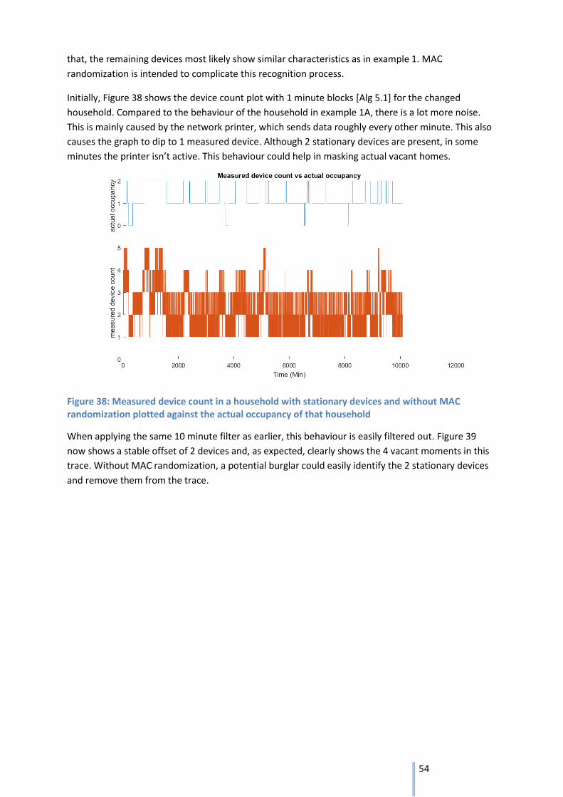
54
that, the remaining devices most likely show similar characteristics as in example 1. MAC
randomization is intended to complicate this recognition process.
Initially, Figure 38 shows the device count plot with 1 minute blocks [Alg 5.1] for the changed
household. Compared to the behaviour of the household in example 1A, there is a lot more noise.
This is mainly caused by the network printer, which sends data roughly every other minute. This also
causes the graph to dip to 1 measured device. Although 2 stationary devices are present, in some
minutes the printer isn’t active. This behaviour could help in masking actual vacant homes.
Figure 38: Measured device count in a household with stationary devices and without MAC randomization plotted against the actual occupancy of that household
When applying the same 10 minute filter as earlier, this behaviour is easily filtered out. Figure 39
now shows a stable offset of 2 devices and, as expected, clearly shows the 4 vacant moments in this
trace. Without MAC randomization, a potential burglar could easily identify the 2 stationary devices
and remove them from the trace.

55
Figure 39: The measured device count of the household averaged over 10 minute intervals, again plotted against the actual occupancy
6.3.4. Example 2B: Normal Household with stationary devices and MAC
randomization
As in example 1B, the previous trace is now regenerated with a MAC randomization scheme. At
random intervals between 3 and 15 minutes, a device switches it’s address. For this trace, which is
the same one as in example 2A, this creates a table of more than 5000 devices. Figure 40 shows that
this creates a lot more noise on the network trace. Not only does the signal look more noisy, the
system also detects up to 8 simultaneous devices while only 5 are available in the household.

56
Figure 40: Measured device count in a household with stationary devices and MAC randomization implemented
By determining the average device count per 10 minute block, a lot of high readings and noise can be
omitted. This filtered trace is shown in Figure 41 below. A lot of noise remains however, and more
importantly, the 4 moments in which the house is empty are barely recognizable compared to other
moments.
Figure 41: Measured device count averaged over 10 minute intervals for a household with stationary devices and MAC randomization.
Assuming that an adversary is unable to stitch traces together and potentially identify the stationary
devices, reliably detecting vacancy has become difficult.

57
Where packet count [Alg 5.2] worked in example 1A, Figure 42 shows that the stationary devices
create a lot of interference on this field as well. Figure 43 shows the same graph but now only a small
part of the packet count scale to improve readability.
Figure 42: The average packet count on the house network per minute, averaged over 10 minute intervals
Figure 43: Lower section of the average packet count on the house network shown, in full, above
The first low point on the graph is an actual absence of all residents. However, the difference with
the other low points is marginal. The other 3 absences aren’t really distinguishable at all.
6.4. Automated vacancy detection on random households Paragraph 6.3 gives an impression on the possibilities of MAC randomization. However it is limited to
1 household layout. To better test the principle, it should be tested on many different households.
This chapter covers the use of the created household generator from Appendix III, Household
modeling and tracking to test different circumstances.

58
The network traces of these generated households are similar to the traces that a burglar would
obtain by eavesdropping on a household. Of each household, a normal and a ‘randomized’ trace is
created. Occupancy is determined from these traces by the use of data processors. If the MAC
randomization scheme is effective, determining vacancy should be difficult from the ‘randomized’
trace.
6.4.1. Network trace processing
De household simulator described earlier generates 1 network trace for all devices combined similar
to what anyone would get when eavesdropping on a network. For a burglar, the next step would be
to determine at which points the household is actually empty. The exact technique, a burglar would
use is always a guess, but some options are worked out below.
Fine grained device count detection Similar to the device count algorithm throughout paragraph 6.3 [Alg 5.1], this algorithm determines the amount of devices that are active simultaneously. The minimum occurring device count during the trace is regarded as the example for an “empty house”. The determined occupancy is checked against the actual occupancy. This creates 4 possible outcomes for each unit of time:
The algorithm predicted a vacant house, the prediction was correct (correct vacant)
The algorithm predicted a vacant house, the prediction was incorrect (false vacant)
The algorithm predicted an occupied house, the prediction was correct (correct occupied)
The algorithm predicted an occupied house, the prediction was incorrect (false occupied)
This algorithm is tested with multiple sets of households:
Households where all occupants have a smartphone and no stationary devices
Households where 83% of occupants have a smartphone (according to statistics) and no stationary devices
Households where 83% of occupants have a smartphone and there is a possibility of having a network printer (10%) and smart thermostat (11.4%).
Each of these test traces are filtered in 1, 5 and 10 minute blocks, both for the original and randomized trace (with a random 3-15 minutes switch time). For each of the 3 household types, a thousand households are simulated and the results are presented in Table 2, Table 3 and Table 4. The figures show the distributions between the predictions and the true/false rates, all with their variation. No stationary device and all residents carry a smartphone
By omitting stationary devices and assuming all residents carry a smartphone, the most optimistic scenario is tested. When network activity is detected, the residents are at home and vice versa. MAC randomization isn’t effective in such a situation as there is no activity present to mask the absence of residents. This is clearly visible in Table 2 below where the scores (with standard deviations) between the normal and randomized traces are identical.

59
Predicted vacant Predicted occupied
% of total % correct % false % of total % correct % false
1 min normal
54.80% 32.96% 67.04% 45,20% 100.00% 0.00%
± 13.06% ± 13.16% ± 13.16% ± 13.06% ± 0.00% ± 0.00%
1 min random
54.80% 32.96% 67.04% 45.20% 100.00% 0.00%
± 13.06% ± 13.16% ± 13.16% ± 13.06% ± 0.00% ± 0.00%
5 min normal
23.72% 78.75% 21.25% 76.28% 100.00% 0.00%
± 12.94% ± 12.76% ± 12.76% ± 12.94% ± 0.00% ± 0.00%
5 min random
23.72% 78.75% 21.25% 76.28% 100.00% 0.00%
± 12.94% ± 12.76% ± 12.76% ± 12.94% ± 0.00% ± 0.00%
10 min normal
18.69% 99.37% 0.63% 81.31% 100.00% 0.00%
± 11,05% ± 1.55% ± 1,55% ± 11.05% ± 0.00% ± 0.00%
10 min random
18.69% 99.37% 0,63% 81.31% 100.00% 0.00%
± 11,05% ± 1.55% ± 1,55% ± 11.05% ± 0.00% ± 0.00%
Table 2: Influence of MAC randomization on 1000 simulated household without stationary devices and all residents carrying a smartphone
The occupied predictions are perfect in this situation, simply because activity equals presence. Meanwhile, vacancy predictions show some interesting effects. In the small timebin test, false vacant rates are very high while one would suspect that presence in this scenario would be easy to predict. With larger time bins, the prediction scores increase dramatically with an almost perfect score when using a 10 minute timebin. The reason for these low scores are relatively simple. Network activity implies presence in this scenario and vacancy implies network silence. But the other way around doesn’t work. Smartphones and other devices aren’t active permanently. Especially when the device isn’t used for an extended period of time (such as, during nights) it goes into a standby mode and only interacts with the network every couple of minutes, as shown below:.
Figure 44: A visual represenation of the intermittend network activity from a smartphone in standby mode
These silent minutes between the peaks are filtered out with the larger timebins. But with the 1 minute timebin, the system detects a constant cycle of absences and presences. As a burglar wouldn’t be interested in per-minute information but only in long-term vacancies, this problem wouldn’t pose a real problem for the burglar in practice.

60
No stationary device and 83% of residents carry a smartphone
This scenario shifts a bit more towards realistic situations by incorporating the possibility of residents
being untraceable by their smartphones. This situation is problematic for a burglar as a seemingly
empty house could have a non-connected resident in it. This situation is somewhat similar to the
standby behaviour explained in the previous scenario and shown in figure Figure 44. The main
difference however, is that the faults aren’t removable by changing the size of the timeslots.
Table 3 shows high and comparable false vacant prediction scores compared to Table 2 when looking
at the 1 minute timebin. But where the false vacant predictions almost disappear with larger
timebins, this scenario keeps an almost 15% false vacant rating with 10 minute timebins. These faults
are caused by untraceable residents and can pose a real problem for burglars using similar
eavesdropping techniques. This difference also causes a higher spread in the results and therefore a
higher standard deviation
Occupied predictions are again perfect. Similar to the previous scenario, the credo “activity is
occupancy” is applicable.
Predicted vacant Predicted occupied
% of total % correct % false % of total % correct % false
1 min normal
60.50% 31.07% 68.93% 39.50% 100.00% 0.00%
± 16.64% ± 13.31% ± 13.31% ± 16.64% ± 0.00% ± 0.00%
1 min random
60.50% 31.07% 68.93% 39.50% 100.00% 0.00%
± 16.64% ± 13.31% ± 13.31% ± 16.64% ± 0.00% ± 0.00%
5 min normal
32.20% 68.22% 31.78% 67.80% 100.00% 0.00%
± 23.59% ± 23.33% ± 23.33% ± 23.59% ± 0.00% ± 0.00%
5 min random
32.20% 68.22% 31.78% 67.80% 100.00% 0.00%
± 23.59% ± 23.33% ± 23.33% ± 23.59% ± 0.00% ± 0.00%
10 min normal
27.21% 85.26% 14.74% 72.79% 100.00% 0.00%
± 24.14% ± 27.15% ± 27.15% ± 24.14% ± 0.00% ± 0.00%
10 min random
27.21% 85.26% 14.74% 72.79% 100.00% 0.00%
± 24.14% ± 27.15% ± 27.15% ± 24.14% ± 0.00% ± 0.00%
Table 3: Influence of MAC randomization on 1000 simulated household without stationary devices and 83% of residents carrying a smartphone
Stationary device and 83% of residents carry a smartphone
Stationary devices were said to be a vital part of masking occupancy. Where network activity
previously ensured occupancy, stationary devices can mask absence by remaining active. This
frustrates occupancy detection. Or at least, that’s the theory.
Where example 2 of chapter 6.3 showed a potential success, it only showed a single situation. When
applied to a thousand random household configurations, the figures are less positive as shown in
Table 4.

61
Predicted vacant Predicted occupied
% of total % correct % false % of total % correct % false
1 min normal
56.26% 30.92% 69.08% 43.74% 98.06% 1.94%
± 19.51% ± 13.25% ± 13.25% ± 19.51% ± 6.34% ± 6.34%
1 min random
55.91% 30.92% 69.08% 44.09% 97.62% 2.38%
± 19.43% ± 13.25% ± 13.25% ± 19.43% ± 6.65% ± 6.65%
5 min normal
31.61% 68.09% 31.91% 68.39% 100.00% 0.00%
± 22.66% ± 23.11% ± 23.11% ± 22.66% ± 0.00% ± 0.00%
5 min random
29.82% 68.10% 31.90% 70.18% 98.22% 1.78%
± 21.95% ± 23.12% ± 23.12% ± 21.95% ± 4.69% ± 4.69%
10 min normal
26.51% 85.03% 14.97% 73.49% 100.00% 0.00%
± 23.08% ± 26.83% ± 26.83% ± 23.08% ± 0.00% ± 0.00%
10 min random
23.74% 85.00% 15.00% 76.26% 97.41% 2.59%
± 22.11% ± 26.84% ± 26.84% ± 22.11% ± 6.14% ± 6.14%
Table 4: Influence of MAC randomization on 1000 simulated household with stationary devices and 83% of residents carrying a smartphone
Compared to the previous scenario without stationary devices, vacant predictions without MAC randomization have become a fraction less reliable while occupancy predictions remain perfect. However, adding MAC randomization shows a change in rates, although small. This wasn’t the case in earlier scenarios. This confirms the need for stationary devices for MAC randomization to have any effect. The effect of MAC randomization on vacancy predictions is negligible with 0.03% difference, but this is understandable. Using stationary devices and MAC randomization to mask absences doesn’t generate false vacancy predictions but hides genuine ones. This effect is visible in the results. When looking at the 10 minute timebins, introducing MAC randomization causes a drop of almost 3 percent in the total vacancy predictions. So although the distribution of the vacancy predictions isn’t changed, there are less of them. This, in turn, means that the occupied predictions become more common. This also introduces false occupied predictions as can be expected. While the house is actually empty, the stationary devices combined with the MAC randomization system create the impression of false occupancy. Remark on measurement uncertainties In general, the figures presented in Table 2 Table 3 and Table 4 show high uncertainty rates. These are caused by the large differences in household compositions. The resident count, their activities and the available devices all have influence on the network traces and therefore the statistics of the predictions. The variations in these predictions are illustrated in Figure 45 where prediction distributions are shown for 100 households separately. Each column represents 1 household with each color representing a prediction outcome:
White: predicted occupied correctly
Blue: predicted occupied while house was vacant
Red: predicted vacant while the house was occupied
Green: predicted vacant, was correct The graph shows the results of a household with stationary devices, a 83% chance of smartphones and a mac randomization scheme implemented. The timeslots for this measurement were 10 minutes long.

62
Figure 45: A visual representation of the spread in prediction scores between 100 simulated households. This graphs shows households with stationary devices, 83% smartphone usage, MAC randomization and 10 minute timebins
6.5. Conclusions MAC addresses are one of the most used identifiers of WiFi devices. Therefore a lot of tracking
systems use these plainly visible addresses. MAC randomization therefore seems like a viable
candidate to prevent the tracking of occupants in a household. With MAC randomizations, a single
devices could show up as dozens during the day. All physical devices combined, this could give a
confusing array of pretended devices (with switched MAC addresses), hiding the actual number of
occupants.
This chapter tried to implement a household simulator to test such a MAC randomization scheme in
a wide variety of households to answer the question:
Is a theoretical implementation of MAC randomization with variable transmission power effective
against occupancy detection in simulated household environments?

63
The aim was to create an initial simulator and then expand it with extra options and devices to create
a better representation of modern households. Unfortunately, time constraints limited the
implementation of extra devices and options.
For the household types that can be created, MAC randomization proves to have little influence on
the trackability of households with a best-case improvement of less than 3% in the generated
households. The main problem being, that an adversary can still determine which devices belong to
that household. Even with MAC randomization, these households show a certain amount of devices
present at any one moment [Alg 5.1]. The tracking of specific devices may be complicated or even
prevented, but the household as a whole proved to be still trackable in this simulator.
For a better representation of the real world, more devices should be added to the simulator with
more traces per device type. Some missing devices in the current simulator are Tablets, Laptops, IoT
devices and game consoles. This was mainly caused by time constraints, but also because of limited
statistics on usage and occurrence.
More scenarios should be added as well, such as leaving your phone at home, having multiple
phones, not always connect to a network and others. These irregular factors complicate traces a lot,
but are realistic in normal households and therefore give a better overview on the effectiveness of
MAC randomization. Creating a realistic simulator however, will take a huge amount of time and
effort. And when considering the marginal influence on the currently simulated scenarios, it is
unlikely that the system will become very effective.

64
7. Research part 4A: MAC randomisation implementations
7.1. Introduction While the concept of mac switching may be interesting, implementing it is another challenge. As it
forms the backbone of local (wireless) communication, changing the MAC address can potentially
give a lot of headaches. This chapter covers potential problems and implementations of such system.
Following the initial research question, this system was intended to be an easily implementable
alternative to cumbersome Wi-Fi protocol changes. This chapter therefore tries to find the answer of
the first part of the stated subquestion:
What possibilities are available for implementing MAC randomization with variable transmission power in current networking protocols?
Apart from possibilities, potential problems of MAC randomization are also mentioned. The variable transmission power part of the question is tackled in chapter 7.
7.2. Problems with MAC switching in active networks Existing MAC randomisation systems as used in some smartphones also switch MAC addresses, but
they only do this while not authenticated with a network. When the device is sending out probe
requests, a packet designed to poll for a known network, it keeps changing the MAC address. But
these packets would only get a reply immediately after the request is send, should that network be in
the vicinity. After a short time, the request can be discarded together with the MAC address. The
only use for the MAC address at this point is for the requested network to send a reply to, stating its
presence. As the device only has to listen for a reply for a short time, discarding the MAC address
afterwards yields no consequences. Only when a reply is received the device has to act. And in most
implementations the device then reverts to its original MAC address and tries to connect.
Sometimes people choose to install a MAC changing program to their computer to prevent tracking.
However these programs usually only switch the address before a network session. So every time the
device connected, it gets a new address. As long as the address remains the same during the
connection, everything will function as normal.
The problems start when someone tries to change its MAC address in an active network. To explain this further, we need to go into some systems used in WiFi networks.
7.2.1. Data encryption
When using unprotected networks, network data encryption isn’t used. However, most networks are secure nowadays. The most used form is the WPA2. As the use of other standards is low and further decreasing every day, this research therefore only covers the WPA standard.

65
Figure 46: Network encryption usage over time with datapoints on januari 2017 [15]
In WPA secured networks, all data above the MAC layer is encrypted. The idea behind this is that the MAC layer is extremely important to filter traffic. When a packet arrives, the MAC address (in the mac layer) is used to determine if the packet is aimed at this device. If not, it’s immediately discarded. Would the MAC layer be encrypted, every device would have to listen to every packet, receive it in full, decrypt it, only to find that most packets are not addressed to it. This would increase computational load and power consumption on a device in a network (especially busy ones).

66
Figure 47: Schematic overview of the steps involved with creating encryption keys in 802.11 WPA networks
The encryption keys used in these kinds of networks are generated when the device authenticates
with the network. The (simplified) procedure is shown in Figure 47: Schematic overview of the steps
involved with creating encryption keys in 802.11 WPA networks. Initially, the Access point has the
Pairwise and Group master key (PMK and GMK) used for respectively unicast and multicast traffic.
After the initial authentication packets, both sizes generate their Nonce values and exchange them.
From these nonces, the Pairwise transient key (PTK) is generated at each end and installed after the
exchange of the GTK+MIC and it’s acknowledgement. The Group Transient Key (GTK) is created by
the access point (if not done already) based on the GMK and a random number and exchanged with
the client device. The message integrity is checked by a message integrity code (MIC).
The unicast encryption key for that session (PTK) is generated on the base of 5 variables: Shared passphrase (PMK)
A nonce value generated by the access point (ANonce)
A nonce value generated by the client station (SNonce)
67
Access point MAC address
Client station MAC address
After the authentication procedure succeeded, both devices have created their set of keys to encrypt and decrypt the network traffic. Should a device change its MAC address, the encryption key would become invalid. No matter if the device keeps using the old keys or would generate new ones, the network router never authenticated with this MAC address and therefore wouldn’t have any keys to decrypt the received packet. In current networks, changing the MAC address simply leads to a lost network connection. The only solution is re-authenticating to establish a new set of keys. This system complicates the implementation of MAC randomization. In further parts of this chapter, several possible systems are proposed to implement a randomization system.
7.2.2. Dynamic Host Configuration Protocol (DHCP)
In addition to the obsolete encryption key problem stated above, the DHCP system could also pose a problem. Normally, when a device associates with a network, it contacts the DHCP server in a network, that server issues an IP address for that device to use while associated with this network. In most consumer grade routers, the available IP address table holds up to 255 addresses of which at least one is reserved for the router itself. These addresses are reserved for that device until it’s no longer needed. Therefore a timeout is set on every address lease. In current consumer grade routers, these lease times are often in multiples of 12 hours. When a device wishes to keep the address for longer, it can renew its address lease before it runs out. The problem however, lies in devices that take on a lot of leases as would happen in a network with MAC randomisation systems. With a lease time of 24 hours as isn’t uncommon, all devices in the network could only switch approximately 250 times per day. With the average device count in a household being above 5 devices this leaves less than 50 switches a day, or approximately every 30 minutes. Although 30 minutes doesn’t sound terrible at first glance, this calculation doesn’t account for visitors and the ever increasing number of connected devices in a household. If it were to function in a current network, it will probably pose problems in the near future. Luckily, a simple solution is available, namely: limit the DHCP lease time. As non-switching devices can just choose to renew their lease, they won’t be really affected apart from some extra management traffic frames. For switching devices, lowering the lease time gives a lot more options for switching. For example, shortening to 30 minutes gives around 2400 possible switches per device per day, or every 36 seconds. When using a more reasonable 10 minutes (for example), the network would be capable of handling households with over 80 devices. Depending on the actual chosen refresh intervals and lease times, this system could always be susceptible to a cat-and-mouse game between the router and the devices. In addition to this, lies the problem of compatibility. Non-switching devices in a switching network will just have to renew their DHCP lease more often which is a normal feature of the network

68
protocol. The problem lies when the situation is reversed and MAC switching devices start entering old-style networks. With a switch time of 10 minutes and a DHCP lease time of 24h, a single MAC switching device will occupy 144 IP addresses out of the available 254 or less. As the goal of the proposed MAC randomization system was to be implemented as a software update in existing devices or to be implemented in the new generation of devices, chances of MAC switching devices to live inside an old-style network are large. Replacement intervals of smartphones are increasing, but on average still happens after just over 2.5 years in the US [16]. Although similar numbers on Wireless routers are virtually non-existent, the trend seems to be to only replace the router when it’s broken, which could be much longer. This could present compatibility issues for many years to come, which is something that should be prevented in this system.
7.3. Implementation 1: Simple network re-authentication As stated in the data encryption section earlier in this chapter, simply changing MAC address of a
device will lead to a network disconnect in the commonly used network types. The most
straightforward implementation of MAC address switching would be to “just” reconnect every time
the address is switched.
As stated in the DHCP section, this could lead to IP address exhaustion and compatibility issues
between new and old devices as it requires changes to both client devices and routers.
In addition to these challenges, there is the problem of user inconvenience. Changing the address
and re-authenticating will take some time in which the user won’t have network access. Especially as
the randomization frequency increases, this can create a lot of inconvenience. A solution for this
could be to detect inactive periods to switch to another address. In the case of a smartphone, this
could be when a user locks the device. This kind of strategies will require comprehensive changes in
the device’s software to be able to detect the appropriate times. Again in the case of the
smartphone, this could lead to a system where applications have something like a ‘busy’ flag. If no
application is “busy “ a switch may occur. This would require a lot of updates to not only the device,
but also numerous applications, again complicating broad adoption. An additional change could be to
authenticate the new MAC address before giving up the old connection. However, the feasibility of
implementing this type of parallel connections would have to be researched further.
Switching to a new network connection also leads to a lot of extra traffic and energy usage. When a
network printer re-associates with a network it will need to advertise its new network location to
enable other devices to print again. Smartphones often synchronize all kind of data to cloud services
when a Wi-Fi connection is established. Changing the MAC address constantly will keep waking these
services, causing extra data transmissions and decrease battery life.
All in all, this implementation, although seemingly simple, proves to be a complicated system with
multiple implementation issues.
7.4. Implementation 2: gratuitous ARP response A gratuitous ARP response gives devices the possibility to take over an existing IP address on a new hardware address. This system is known to be used in some redundant server systems. Imagine:

69
Server A being the active server with MAC address A. All internet traffic finds that server via IP address 1.
Server B is on standby with MAC address B
Normally, all incoming traffic is routed to server A. As soon as server B finds out that server A has a problem it sends a gratuitous ARP request to the network: IP address 1 is now at MAC B. The network switches, router update their routing tables with this information and internet traffic is now routed to server B. In the MAC randomisation concept, the same system is desired but both MAC addresses belong to the same physical device. Unfortunately, the explained routine works on wired networks. In a wireless network, the ARP packet will be send as a broadcast transmission and therefore encrypted with the so called “Group temporal key” which is the same across all devices and therefore not influenced by the changing MAC. Unfortunately, the unicast traffic (point-to-point) uses a unique key that is MAC address dependent and thus bringing back the earlier stated problem with WPA encryption. The gratuitous ARP response, however, isn’t always a supported packet. Although rather undocumented for consumer grade equipment, some enterprise grade equipment [17] normally ignores gratuitous ARP responses. This could pose problems should this technique be widely implemented in Wi-Fi networks.
7.4.1. Implementation 2.1: WPA keylist
Normally, the AP and device use the generated Nonce values to generate the PTK (the encryption key for the unicast traffic between them). But instead of storing only the PTK, what if both devices store the values used to generate that key as well?
When the device switches MAC address, it can retake the old nonce values, known passphase and the AP’s MAC address add its new MAC address and calculate new PTK values for this MAC.
The network router already detected the upcoming switch by the gratuitous ARP response send out earlier. It has a list of all known devices with their used nonces and such. From the DHCP table it can work out which MAC address was using that IP address originally and therefore which values it should use to generate the PTK. It takes those values with the new MAC address, constructs the new PTK and is again able to transmit and receive encrypted data with this device on a new MAC address.
7.4.2. Implementation 2.2: Initiate secondary connection
The WPA key issue can also be mitigated by first authenticating the new MAC address with the
access point and afterwards send the gratuitous ARP response. This implementation is similar to the
one used in wired networks. Both interfaces (although in this case, they belong to the same device)
are registered and 1 IP address is shared between the two of them.
When a device wants to switch address, it first authenticates to the network with the new MAC
address but doesn’t request a DHCP lease (IP address). This means that a set of genuine WPA keys
are created like any other device would do when connecting to the network. After this step, the

70
device sends out the required gratuitous ARP response to indicate that the existing IP address can
now be found at the new MAC address.
This system potentially allows a device to retain its IP address to minimize user inconvenience. If
both MAC addresses are kept active, the system could even bounce between addresses multiple
times before discarding one of them and initiating a new one.
7.5. Consideration Of the three implementations posted above, implementation 2.2 is the most promising. Assuming
gratuitous ARP replies are generally supported in networks this system allows for easy switching
without too much user inconvenience.
Implementation 2.1 requires changes to both sides of the network, which complicates adoption
times. This implementation is also the most prone to compatibility problems. If the router isn’t
compatible, a switch made by a client device will result in the loss of network access. A device should
therefore have some measure to detect compatible networks. Implementation 1 is the simplest to
implement, but involves the most user inconvenience as the device needs to restart all network
connections at every switch. This increases energy consumption and potentially disrupts user
activities.
7.6. Other Factors and problems
7.6.1. Usable MAC range
MAC addresses are normally distributed by the IEEE standards association. Manufacturers buy a block of addresses and distribute them across the produced networking devices. Normally the MAC address is 48 bits long leading to over 280 trillion possible combinations. However, not all are usable. The most common one is the broadcast address with all ones ( FF:FF:FF:FF:FF:FF in hexadecimal notation). This address is accepted by all devices and should therefore not be used to identify a specific device.
Additionally, least significant bit of the first octet is reserved as the multicast bit. Setting this bit to 1 indicates that the packet is send at a group address instead of a single device. For the sake of compatibility, this bit should be left alone when randomizing the MAC address.
Next to the multicast flag is the “locally administered” (LA) flag. With all IEEE distributed addresses, this bit is zero indicating that the address is globally unique. Setting this bit indicates a locally administered algorithm outside the IEEE program. In the light of this MAC randomization scheme, it would seem logical to set the LA flag in all randomized addresses to prevent address collisions with said-to-be globally unique addresses. When such randomizations system would become common, the IEEE is likely to demand this from its clients (the NIC manufacturers) to prevent problems with the original IEEE standards. Unfortunately, this also has the effect that any eavesdropper can easily separate randomized and “original” addresses. This may not be of great help in tracking the presence of the users, but does indicate that a MAC randomization scheme is in use. With the multicast and LA bit fixed, 46 bits remain to be randomized giving just above 70 trillion address options.

71
7.6.2. MAC collisions
With more than 70 trillion possible addresses collisions aren’t really likely. But if every device is randomly switching its MAC address, it is could happen eventually. This could lead to connection problems in a network as this address is used to direct traffic to the right recipient. However, the chances of this problem occurring are very low:
Say a household has 5 active devices and the system would use the full 46 “free” bits for randomization. The chance of 1 device address colliding with one of the other 4 is 5.7*10-14 %. With a switch every minute, an address collision would, on average, happen once every 33 million years.
However, with 3 billion devices shipping in 2017 and 8 billion considered active [18], sticking to the 5 device average per household and keeping the birthday paradox in mind, it would give a collision somewhere in the world every 3.4 days. Although these calculations hold barely any statistical value, it shows the need to address this collision problem to make the randomization scheme viable for wide implementation. Some of the possible situations are simple to tackle. For example, the use of an non-switching device in a switching network. The non-switching device wouldn’t be aware of (the possibility of) any other device using its MAC address and will just authenticate potentially causing a collision. The switching device couldn’t have prevented this with any scanning before his switch as the non-switching device wasn’t present. However, using locally administered addresses (as will be likely, by pressure of the IEEE association), a collision with non-switching devices can never occur. Their addresses are in a separate address block.
Between switching devices, the problem can be somewhat mitigated by checking the device’s ARP table (containing a list of known devices in the network with their MAC addresses) before switching. However this only works for devices that have been recently communicating with the soon-to-be-switching device. Otherwise they won’t be in the ARP table.
As a last resort, the device awaiting a MAC switch could emit a reverse ARP packet to check for the usage of the desired MAC address. Where a normal ARP packet seeks to get the MAC address from a known IP, the reversed ARP packet can be used the other way around. Should another device using that MAC be present in range, it should reply on said ARP request. But it gets more complicated. Although the contents of an ARP request is encrypted, an adversary may be able to distinguish it in a network trace by its (fixed) size. An adversary could check the trace around the time of a “disappearing” device and look for an ARP sized packet containing the source address of the old device and the destination of (one of the) new devices. This way, the old device basically tells the burglar to which MAC address it hopped, defeating the whole system.
In the Gruteser & Grunwald [5] research, a solution is given where a device performs a double switch. First to a randomly selected MAC address without collision detection to prevent disclosing the switch. Then from the new device address, perform the required ARP request to another randomly selected address. Then switch over again, assuming no reply was received. This omits the link between address A and C and, due to its short usage and limited amount of generated traffic (ARP request only), the “unprotected” address B won’t give much trouble when a collision would occur.
7.6.3. Packet sequence number
The 802.11 MAC layer holds a 2 byte data field holding a fragment (4 bit) and sequence (12 bit) number. The first one is used to identify different fragments of a transmission if it’s divided into

72
multiple packets. The latter one is an incrementing field enumerating all send packets. As the MAC layer is unencrypted, this number is clearly visible for any eavesdropping device. Although a MAC address was switched and the transmission power altered, the sequence number could easily aid in connecting the 2 “devices” together.
When a device changes MAC address, this number should be at least reset or maybe even randomized. Power cycling the network controller could have that effect, but this creates extra delay on every switch. Unfortunately, not much information is available on the possibilities to alter this field from within the device’s software. This is important for this solution to be easily implementable and usable.
Figure 48: 802.11 MAC layer contents with the fragment and sequence numbers shown in the center
7.6.4. Traffic pattern recognition
Most networks are protected nowadays and therefore feature data encryption, that hasn’t stopped people from trying to track certain aspects. A field that has been studied often is the recognition of devices, device types or certain services by their traffic patterns.
In [19] a trace of 15 minutes sufficed to identify a smartphone in a network with a probability of 90% based on the behaviour of popular services.
To top that, other researchers [20]were able to identify patterns of specific applications such as chatting, online gaming and browsing with an accuracy of around 80% in only 5 seconds of network trace data. With a minute of data, this accuracy increased to 90% and higher.
With these kind of possibilities, MAC randomisation alone is only an inconvenience. With a bit of signal analysis an adversary could still track a lot of information within a household. An additional requirement to battle this possibility is to remove identifying characteristics from data traffic such as packet size and interval. To hide packet size, fixed packet lengths and padding could be used as is done in the TOR network which sets all cells to a 512 byte size. This would require a lot of changes to network software of all sorts of devices.
The packet interval is another issue. Some services require a lot more data than others. Streaming a high definition video will require a lot and/or large packets, while a service like WhatsApp will only generate a fraction of this. Other services like online gaming could have a high demand on the side of

73
latency of the communication. Implementing limitations on packet sizes and frequency will affect these parameters and therefore their services and the experience of the user.
7.6.5. Spectral fingerprinting
Although less likely, an adversary could even track devices simply by their spectral fingerprints. Small differences in hardware design and component tolerances in production create device specific signal characteristics that could be used to track the device. Some researchers [21] were able to identify devices with an accuracy of 80% by their spectral fingerprints. As this type of tracking requires advances signal processing, it’s less likely to be used for the purpose of burglary.

74
7.7. Conclusion This research tries to find an easy to implement technique for MAC randomization following the
research subquestion of:
What possibilities are available for implementing MAC randomization in current networking protocols?
Ideally, the system would only require a software update at the client side (e.g. smartphone, printer
etc.) and would have little influence on connectivity for the user.
The best found solution for this would be implementation 2.2, that uses reverse ARP replies to
transfer the active IP address to a new MAC address. This implementation doesn’t require changes to
the network router, like implementation 2.1 does. It does however, require networking equipment to
allow for gratuitous ARP replies. The acceptance of these packets is reasonably unknown. Some
enterprise grade equipment doesn’t allow for them, unless specifically enabled.
Although chances are reasonably low, detecting and preventing MAC collisions is also a problem. The
ARP packets that could be used to detect collisions would also reveal details of the address switch to
any eavesdropper. The solution of using a dummy address to buffer between the old and new
address largely solves this.
Although implementation 2.2 is reasonably easy to implement, for optimal user convenience it
requires knowledge of the actual device usage to determine optimal switching moments. But even if
this would be added to the implementation, there are still a lot of issues that limit the effect of a
MAC randomization scheme.
Traffic pattern recognition techniques can potentially detect key parameters of devices between switches with traces of only minutes or less in length.
For a more advanced burglar, spectral fingerprinting could be used to identify devices regardless of address.
Sequence numbers in the MAC header need masking, resetting or randomizing possibilities or any eavesdropper can just stitch randomized sessions together.
Triangulation techniques can be used to identify stationary devices. And, as shown in chapter 6, detecting occupancy is quite simple without stationary devices
In total, a client side implementation of MAC randomization may be feasible. But the actual
effectivity of the technique is questionable. An adversary has a legion of potential solutions to try
and reverse the randomization. And even if he/she couldn’t link the virtual devices together, it isn’t
said that occupancy detection won’t work.

75
8. Research part 4B: Variable transmission power implementation
8.1. Introduction As shown in chapter 5, changing the MAC address alone leaves the possibility for an adversary to link
devices back together based on their signal strength. Especially stationary devices are a potentially
easy prey for such comparisons. Variations in transmission power proved to be a viable way to
interfere with this comparison and complicate the tracking of specific devices in a network. This
chapter covers the implementation and challenges of transmission power adjustments in client
devices to answer the second part of the question:
What possibilities are available for implementing MAC randomization with variable transmission power in current networking protocols?
Simply changing the transmission power to an arbitrary value may work against tracking, but doesn’t
consider network connectivity. Depending on the house, the used equipment and the location of the
equipment certain minimum power levels are required to maintain a stable connection. However,
the 802.11 standard doesn’t include any means of determining network strength. So, until
connections start failing, a device aren’t aware of any limits.
8.2. Possible implementations Prior research was conducted on the use of variable transmission power. This research can be found
in Appendix IV: Report of prior literature research under chapter 4. Several algorithms have been
developed, some for Wi-Fi networks, others for wireless sensor networks. However most algorithms
require changes to network protocols or devices making implementation difficult.
Ideally, acknowledgement messages from devices contain some information about the received
signal strength. This way, a client device can easily manage its boundaries on transmission power.
Unfortunately, this data isn’t available in the 802.11 standard. This leaves 3 options:
8.2.1. Implementation 1: Change the 802.11 standard to include the required RSSI
data
As the whole proposal is based on an easy to implement solution without protocol changes, this is obviously not a feasible solution.
8.2.2. Implementation 2: Embed RSSI feedback in higher network layers
This system is also used in the variable transmission network COMPOW [22] where a process is run on each machine that exchanges data on RSSI values via normal data packets. This implementation is directly compatible with the 802.11 protocol but requires both sides of the transmission to support the system. Otherwise no feedback is given or the given feedback is ignored.
8.2.3. Implementation 3: Track packet loss and received RSSI values
Without feedback possibility, a device can only find its power limitations by trial and error. For a client device, the received RSSI values from the router could give some insight in network layout. Although the transmission power of the router is unknown, a low received signal strength is likely to indicate high signal loss or long transmission path in a transmission and therefore a high power

76
requirement for the client device. Also, tracking the received RSSI values can help in detecting device movement and therefore changed limits. However, the actual boundary can only be found by missing acknowledgements on send packets and thus packet loss.
The higher level client process looks like the more robust candidate. It allows for a better
determination of minimum transmission power and can quickly adjust for moving devices.
Unfortunately, it does require both sides of the connection to embed this process. As this system is
intended as an implementation on new devices or, even better, via a software update, there will be a
lot of cases where not all devices are compliant.
The ultimate choice would be dependent on the chosen implementation of the MAC randomization.
Is that system is only a client side update, then so should the transmission power system be. In that
case, tracking packet loss and received RSSI is the only option. Alternatively, should the system
require changes on both sides, implementation 2 can be chosen without much problems. As the MAC
randomization system is then likely to only function when both sides are compliant, the signal
strength functionality would then be present at both ends at well.
8.3. Limitations
8.3.1. Fine grained transmission power control
One of the requirements for a proper implementation of variable transmission power for this purpose is the possibility to control the transmission control in a fine-grained manner. Without this, choosing a setting lower than maximum power could quickly put devices at or over the edge of effective wireless range. This means devices will be often forced to stay at the same power level and thus remain vulnerable for a SNR comparison attack. Fine grained transmission power control also gives a better chance of hiding the connection between different MAC address sessions. If only a few options are available, a lot of sessions would still have comparable SNR values. Not so much of a problem for mobile devices, but stationary ones could remain relatively easily identifiable. Unfortunately, information on transmission power control across commonly used hardware isn’t publicly available. Therefore no real assessment can be made on the usability of such system on current hardware.
8.4. Problems
8.4.1. Eavesdropping with triangulation
Up until this part, the eavesdropping scheme of a burglar was visioned as a single device placed
somewhere in the vicinity of a household. A lowered transmission power could then translate to the
same SNR ratio as when the device would have moved. Unfortunately, this difference may be
relatively easy to distinguish by placing multiple devices throughout a neighbourhood.
In an ideal situation (from the burglar’s perspective), 3 or more devices are placed evenly around a
home. A stationary device is picked up by all devices with a certain signal strength depending on the
distance and materials between them. As long as the device remains stationary, the received signal
strength values remain similar as well. When a device would lower its transmission power, the signal
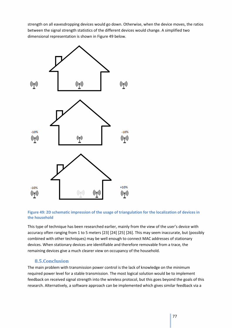
77
strength on all eavesdropping devices would go down. Otherwise, when the device moves, the ratios
between the signal strength statistics of the different devices would change. A simplified two
dimensional representation is shown in Figure 49 below.
Figure 49: 2D schematic impression of the usage of triangulation for the localization of devices in the household
This type of technique has been researched earlier, mainly from the view of the user’s device with
accuracy often ranging from 1 to 5 meters [23] [24] [25] [26]. This may seem inaccurate, but (possibly
combined with other techniques) may be well enough to connect MAC addresses of stationary
devices. When stationary devices are identifiable and therefore removable from a trace, the
remaining devices give a much clearer view on occupancy of the household.
8.5. Conclusion The main problem with transmission power control is the lack of knowledge on the minimum
required power level for a stable transmission. The most logical solution would be to implement
feedback on received signal strength into the wireless protocol, but this goes beyond the goals of this
research. Alternatively, a software approach can be implemented which gives similar feedback via a

78
higher network layer and a special daemon on both devices. This requires changes to both sides, but
allows the devices to adjust their power levels more precise with less risk of lost connections. If the
solution has to be client side only, the device can only try to find the boundaries of signal strength by
tracking packet loss and SNR values of incoming packets.
At the beginning of this chapter, the applicable research subquestion was set to be:
What possibilities are available for implementing variable transmission power in current networking protocols?
The choice of optimal solution should be based around the implementation of the MAC
randomization scheme itself. Should that system require changes on both sides of the connection,
then it’s easy to add SNR feedback daemons as well. Otherwise, the only viable option is the client
side only solution although it is less than ideal.
Apart from the choice of implementation, the system relies on the availability of fine grained
transmission power control. Unfortunately, information on this part isn’t available. This has to be
researched further if an implementation is going to be made. Manufacturers of common networking
equipment could aid in achieving this data.

79
9. Final conclusion The joint part of this research was intended to prove the risk of Wi-Fi occupancy tracking in
households. This field hasn’t been researched much. Unfortunately, the chosen environment
featuring a shared Wi-Fi network proved to be too difficult to work with. The first part of the
research was to gather data from participating households and extract the devices belonging to them
from the network traces. However, the signal strength and other aspects weren’t enough to make a
reliable distinction. This prevented the second and most vital part of the research question to be
answered:
Is it possible to reliably track occupancy in a household with passive eavesdropping on its Wi-
Fi traffic?
As no reliable distinction between devices that did or did not belong to that household could be
made, no real conclusion of this question could be derived. Devices that visually matched the
schedule gave reasonably high scores with an overall prediction score of 87.8% (+/- 9.75%) across 25
datasets. The rest of the, in total, 55 datasets were lost due to various problems with hardware,
software or because no visually matching devices were found in the data.
Although this joint research didn’t produce the proof wanted to show the potential risk people run, it
didn’t influence the individual research into a solution. The individual research focussed on using
MAC address randomization and variable transmission power to prevent Wi-Fi occupancy tracking
without requiring changes to network protocols.
This part was split into multiple steps, starting with recreating a similar research performed on a
public Wi-Fi network trace. By recreating these steps and adding the part on variable transmission
power, the results could be compared. Unfortunately, the research paper lacked detail in the
descriptions of taken actions requiring some guesswork and comparing the results. This gave some
idea of which steps were taken, but not enough for a satisfying conclusion. The system did improve
the odds (from a victim’s perspective), but not with comparable figures. As the circumstances
differed vastly from the intended ones, normal households, this wasn’t regarded a large problem.
The next part was to try and prove the use of the proposed system in a household environment. The
simulator created for this showed that the proposed system was unable to prevent occupancy
tracking. However, due to time constraints, the simulator wasn’t a complete reflection of realistic
households. The amount and types of devices were limited as well as usage scenarios. For a final say,
the simulator should be expanded but so far, the outlook is grim.
As a last step, the practical implementation was researched. This was firstly to assess the technical
possibilities for such a system. Using gratuitous ARP to enrol new MAC addresses looks to be the best
option when user inconvenience is also taken into account. It does require network devices to allow
this use, which isn’t well documented. Additionally, it does leave a lot of potential ways to reconnect
different MACs of the same device. Variable transmission power proved to be difficult as well.
Without protocol changes, no signal strength feedback is available allowing for dropped connections
due to too-low power settings. A daemon running on the device and communicating via higher
network layers is possible, but still requires both sides to be compatible.

80
Apart from feasibility, the research also uncovered some problems with these implementations,
mainly that the system still leaves a lot of tracking possibilities caused by the network protocol (I.e.
sequence numbering), the device (spectral fingerprints) and the user’s activities (traffic patterns).
Altogether, MAC randomization with variable transmission power cannot be regarded as a viable
solution against Wi-Fi MAC tracking in households. The effect so-far is limited at best. And even if the
system is improved, implementation is problematic and there are multiple issues remaining that
stand in the way of hiding actual occupancy.
9.1. Future work Although the proposed system seems broken from the start, some directions could be explored
further. The problems that occurred in the shared research part prevented a definitive conclusion
into the risk of burglars tracking household occupancy via Wi-Fi signals. As stated in the conclusion of
the applicable chapter, this research could be rerun with better circumstances such as:
Normal household environments without a shared network
Extra features on the measurement equipment such as a real-time clock and a way to keep
tabs on the systems operation
More efficient distribution and retrieval of the devices
The created household simulator could be expanded to better reflect actual households. This will
involve:
More device types that are commonly seen in households, such as tablets and game consoles
Multiple traces per device type, as network activity will probably vary between brands and
models
More realistic situations like forgetting a phone, not being connected to a network, visitors
connecting to the network and such.
The improved simulator could be used to give a realistic overview of the possibilities of the proposed
, but also other solutions.
To complicate a burglar’s attempt to recombine “switched” devices, MAC switching systems could
be improved by using multiple active sessions per device to hide actual switches. This would,
however, have a lot of impact on devices, networks and applications.
Finally, other ways of preventing occupancy tracking can be researched in general. Although the
proposed solution may have panned out to be ineffective, that doesn’t mean other solutions aren’t
available.

81
10. References
[1] A. B. M. Musa and J. Eriksson, “Tracking unmodified smartphones using wi-fi monitors,” in
Proceedings 10th ACM Conference on Embedded Network Sensor Systems, Toronto, Ontario, Canada,
2012.
[2] S. Knapton, “The Telegraph,” 27 December 2016. [Online]. Available:
https://www.telegraph.co.uk/science/2016/12/27/high-street-shops-secretly-track-customers-using-
smartphones/.
[3] Centraal bureau voor de Statistiek, “Geregistreerde diefstallen; diefstallen en verdachten, regio,”
2010-2016. [Online]. Available:
http://statline.cbs.nl/Statweb/publication/?VW=T&DM=SLNL&PA=83651NED&D1=0&D2=0&D3=0,13-
15,l&D4=0&D5=a&HD=171023-1448&HDR=G4,G3,G1,T&STB=G2.
[4] W. Lamet and K. Wittebrood, “Nooit meer dezelfde: gevolgen van misdrijven voor slachtoffers,” Den
Haag, 2009.
[5] M. Gruteser and D. Grunwald, “Enhancing Location Privacy in Wireless LAN Through Disposable
Interface Identifiers: A Quantitative Analysis,” Mobile Networks and Applications, vol. 10, no. 3, pp.
315--325, June 2005.
[6] R. Lubben, T. Kers and R. Löwik, “Digital stakeout analysis,” in N.A., Enschede, 2015.
[7] P. Najafi, A. Georgiou, D. Shachneva and I. Vlavianos, “Privacy Leaks from Wi-Fi Probing,” University
college London, London, 2014.
[8] B. Bloessl, C. Sommer, F. Dressier and D. Eckhoff, “The scrambler attack: A robust physical layer attack
on location privacy in vehicular networks,” in in proceedings of the 2015 International Conference on
Computing, Networking and Communications (ICNC), Garden Grove, CA, 2015.
[9] M. Cunche, “I know your MAC address: targeted tracking of individual using Wi-Fi,” Journal of
Computer Virology and Hacking Techniques, vol. 10, no. 4, pp. 219-227, 2014.
[10] M. Malekzadeh, A. Azim, A. Ghani, Z. A. Zulkarnain and Z. Muda, “Security Improvement for
Management Frames in IEEE 802.11 Wireless Networks,” vol. 7, no. 6, pp. 276-284, 2007.
[11] B. Greenstein, D. McCoy, J. Pang, T. Kohno, S. Seshan and D. Wetherall, “Improving wireless privacy
with an identifier-free link layer protocol,” in Proceedings of the 6th international conference on
Mobile systems, applications, and services, New York, 2008.
[12] Boston university school of public health, [Online]. Available: http://sphweb.bumc.bu.edu/otlt/MPH-
Modules/BS/BS704_Power/BS704_Power2.html.

82
[13] “Caida,” 08 11 2006. [Online]. Available: http://imdc.datcat.org/collection/1-004Y-
P=SIGCOMM+2001+Conference+Wireless+Trace#annotations.
[14] EXFO OiDViEW, “OIDVIEW,” [Online]. Available: http://www.oidview.com/mibs/762/KBRIDGE-
MIB.html.
[15] “WiFi Encryption Over Time from Wigle.net,” [Online].
[16] A. Meola, “Business insider,” 30 June 2016. [Online]. Available:
http://www.businessinsider.com/people-are-taking-longer-to-upgrade-their-smartphones-2016-
6?international=true&r=US&IR=T.
[17] Juniper Networks, “Juniper Networks,” [Online]. Available:
https://kb.juniper.net/InfoCenter/index?page=content&id=KB24349.
[18] WiFi Alliance, 4 January 2017. [Online]. Available: https://www.wi-fi.org/news-events/newsroom/wi-
fi-alliance-publishes-7-for-17-wi-fi-predictions.
[19] T. Stöber, M. Frank, J. Schmitt and I. Martinovic, “Who do you sync you are?: smartphone
fingerprinting via application behaviour,” in Proceedings of the sixth ACM conference on Security and
privacy in wireless and mobile networks, Budapest, Hungary, 2013.
[20] F. Zhang, W. He, X. Liu and P. G. Bridges, “Inferring users' online activities through traffic analysis,” in
Proceedings of the fourth ACM conference on Wireless network security, Hamburg, Germany, 2011.
[21] W. C. Suski II, M. A. Temple, M. J. Mendenhall and R. F. Mills, “Using Spectral Fingerprints to Improve
Wireless Network Security,” in IEEE GLOBECOM 2008 - 2008 IEEE Global Telecommunications
Conference, 2008.
[22] S. Narayanaswamy, V. Kawadia, R. S. Sreenivas and P. R. Kumar, “Power Control in Ad-Hoc Networks:
Theory, Architecture, Algorithm and Implementation of the COMPOW Protocol,” in in European
Wireless Conference, 2002.
[23] N. L. Dortz, F. Gain and P. Zetterberg, “WiFi fingerprint indoor positioning system using probability
distribution comparison,” in In proceedings for the 2012 IEEE International Conference on Acoustics,
Speech and Signal Processing (ICASSP), Kyoto Japan, 2012.
[24] E. Mok and G. Retscher, “Location determination using WiFifingerprinting versus WiFi trilateration,”
in Journal of Location Based Services, 1 ed., Taylor & Francis, 2007, pp. 145-159.
[25] E. E. L. Lau and W. Y. Chung, “Enhanced RSSI-Based Real-Time User Location Tracking System for
Indoor and Outdoor Environments,” in In proceedings of the 2007 International Conference on
Convergence Information Technology (ICCIT 2007), 2007.
[26] G. Zàruba, M. Huber, F. A. Kamangar and I. Chlamtac, “Indoor location tracking using RSSI readings

83
from a single Wi-Fi access point,” Wireless Networks, vol. 13, no. 2, pp. 221-235, 2007.
[27] C. Matyszczyk, Cnet.com, 8 februari 2015. [Online]. Available:
https://www.cnet.com/news/samsungs-warning-our-smart-tvs-record-your-living-room-chatter/.
[28] B. Michele and A. Karpow, “Watch and be watched: Compromising all Smart TV generations,” in In
proceedings of the 2014 IEEE 11th Consumer Communications and Networking Conference (CCNC),
2014.
[29] Zebra Technologies, “Analysis of iOS 8 MAC randomization on locationing”.
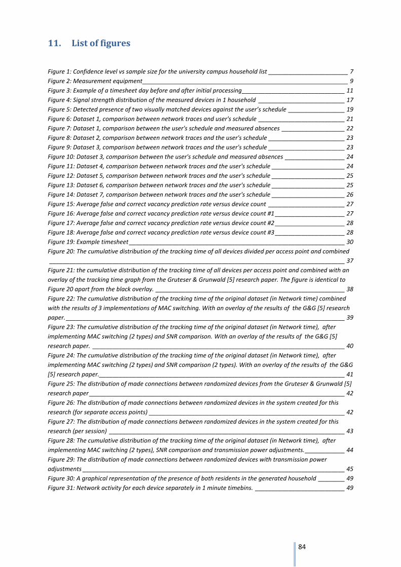
84
11. List of figures
Figure 1: Confidence level vs sample size for the university campus household list ________________________ 7
Figure 2: Measurement equipment ______________________________________________________________ 9
Figure 3: Example of a timesheet day before and after initial processing _______________________________ 11
Figure 4: Signal strength distribution of the measured devices in 1 household __________________________ 17
Figure 5: Detected presence of two visually matched devices against the user’s schedule _________________ 19
Figure 6: Dataset 1, comparison between network traces and user's schedule __________________________ 21
Figure 7: Dataset 1, comparison between the user's schedule and measured absences ___________________ 22
Figure 8: Dataset 2, comparison between network traces and the user's schedule _______________________ 23
Figure 9: Dataset 3, comparison between network traces and the user's schedule _______________________ 23
Figure 10: Dataset 3, comparison between the user's schedule and measured absences __________________ 24
Figure 11: Dataset 4, comparison between network traces and the user's schedule ______________________ 24
Figure 12: Dataset 5, comparison between network traces and the user's schedule ______________________ 25
Figure 13: Dataset 6, comparison between network traces and the user's schedule ______________________ 25
Figure 14: Dataset 7, comparison between network traces and the user's schedule ______________________ 26
Figure 15: Average false and correct vacancy prediction rate versus device count _______________________ 27
Figure 16: Average false and correct vacancy prediction rate versus device count #1 _____________________ 27
Figure 17: Average false and correct vacancy prediction rate versus device count #2 _____________________ 28
Figure 18: Average false and correct vacancy prediction rate versus device count #3 _____________________ 28
Figure 19: Example timesheet _________________________________________________________________ 30
Figure 20: The cumulative distribution of the tracking time of all devices divided per access point and combined
_________________________________________________________________________________________ 37
Figure 21: the cumulative distribution of the tracking time of all devices per access point and combined with an
overlay of the tracking time graph from the Gruteser & Grunwald [5] research paper. The figure is identical to
Figure 20 apart from the black overlay. _________________________________________________________ 38
Figure 22: The cumulative distribution of the tracking time of the original dataset (in Network time) combined
with the results of 3 implementations of MAC switching. With an overlay of the results of the G&G [5] research
paper. ____________________________________________________________________________________ 39
Figure 23: The cumulative distribution of the tracking time of the original dataset (in Network time), after
implementing MAC switching (2 types) and SNR comparison. With an overlay of the results of the G&G [5]
research paper. ____________________________________________________________________________ 40
Figure 24: The cumulative distribution of the tracking time of the original dataset (in Network time), after
implementing MAC switching (2 types) and SNR comparison (2 types). With an overlay of the results of the G&G
[5] research paper. __________________________________________________________________________ 41
Figure 25: The distribution of made connections between randomized devices from the Gruteser & Grunwald [5]
research paper _____________________________________________________________________________ 42
Figure 26: The distribution of made connections between randomized devices in the system created for this
research (for separate access points) ___________________________________________________________ 42
Figure 27: The distribution of made connections between randomized devices in the system created for this
research (per session) _______________________________________________________________________ 43
Figure 28: The cumulative distribution of the tracking time of the original dataset (in Network time), after
implementing MAC switching (2 types), SNR comparison and transmission power adjustments. ____________ 44
Figure 29: The distribution of made connections between randomized devices with transmission power
adjustments _______________________________________________________________________________ 45
Figure 30: A graphical representation of the presence of both residents in the generated household ________ 49
Figure 31: Network activity for each device separately in 1 minute timebins. ___________________________ 49

85
Figure 32: Measured and actual occupancy in the non-randomizing household with 1 minute timebins. _____ 50
Figure 33: Measured and actual occupancy in the non-randomizing household based on the maximum value of
10 minute timebins. _________________________________________________________________________ 50
Figure 34: The packetcount of all devices combined in the household in 1 minute timebins ________________ 51
Figure 35: Network activity vs. the actual number of occupants in the household, based on the total
packetcount. ______________________________________________________________________________ 52
Figure 36: Measured number of active devices per minute in a MAC randomizing household without stationary
devices ___________________________________________________________________________________ 53
Figure 37: Measured number of active devices averaged over 10 minute intervals in a MAC randomizing
household without stationary devices __________________________________________________________ 53
Figure 38: Measured device count in a household with stationary devices and without MAC randomization
plotted against the actual occupancy of that household ____________________________________________ 54
Figure 39: The measured device count of the household averaged over 10 minute intervals, again plotted
against the actual occupancy _________________________________________________________________ 55
Figure 40: Measured device count in a household with stationary devices and MAC randomization implemented
_________________________________________________________________________________________ 56
Figure 41: Measured device count averaged over 10 minute intervals for a household with stationary devices
and MAC randomization. _____________________________________________________________________ 56
Figure 42: The average packet count on the house network per minute, averaged over 10 minute intervals __ 57
Figure 43: Lower section of the average packet count on the house network shown, in full, above __________ 57
Figure 44: A visual represenation of the intermittend network activity from a smartphone in standby mode __ 59
Figure 45: A visual representation of the spread in prediction scores between 100 simulated households. This
graphs shows households with stationary devices, 83% smartphone usage, MAC randomization and 10 minute
timebins __________________________________________________________________________________ 62
Figure 46: Network encryption usage over time with datapoints on januari 2017 [15] ____________________ 65
Figure 47: Schematic overview of the steps involved with creating encryption keys in 802.11 WPA networks _ 66
Image self-created with websequencediagrams.com. Sources include: https://en.wikipedia.org/wiki/IEEE_802.11i-2004 http://www.hitchhikersguidetolearning.com/2017/09/17/eapol-4-way-handshake/
Figure 48: 802.11 MAC layer contents with the fragment and sequence numbers shown in the center _______ 72
Source: http://www.itcertnotes.com/2011/05/ieee-80211-frame-types.html Figure 49: 2D schematic impression of the usage of triangulation for the localization of devices in the household
_________________________________________________________________________________________ 77
Figure 53: Visualised network trace of a Philips 40PFK5500/12 smart TV _____________________________ 105
Figure 54: Part of the visualised network trace of a Philips 40PFK5500/12 smart TV ____________________ 105
Figure 55: Visualised network trace of a Nefit Nest smart thermostat ________________________________ 106
Figure 56: Visualised network trace of a Sony Xperia Z5 compact smartphone running Android 7.0 ________ 107
Figure 57: Visualised network trace of a Sony Xperia Z5 compact smartphone running android 7.0 in standby
during sleep hours _________________________________________________________________________ 107
Figure 58:Visualised network trace of a Hewlett Packard Photosmart C4780 network printer _____________ 108

86
12. List of tables
Table 1: User presence results with their respective standard deviations ............................................................ 19
Table 2: Influence of MAC randomization on 1000 simulated household without stationary devices and all
residents carrying a smartphone .......................................................................................................................... 59
Table 3: Influence of MAC randomization on 1000 simulated household without stationary devices and 83% of
residents carrying a smartphone .......................................................................................................................... 60
Table 4: Influence of MAC randomization on 1000 simulated household with stationary devices and 83% of
residents carrying a smartphone .......................................................................................................................... 61
Table 5: Overview of missing SNR values by classification .................................................................................. 101
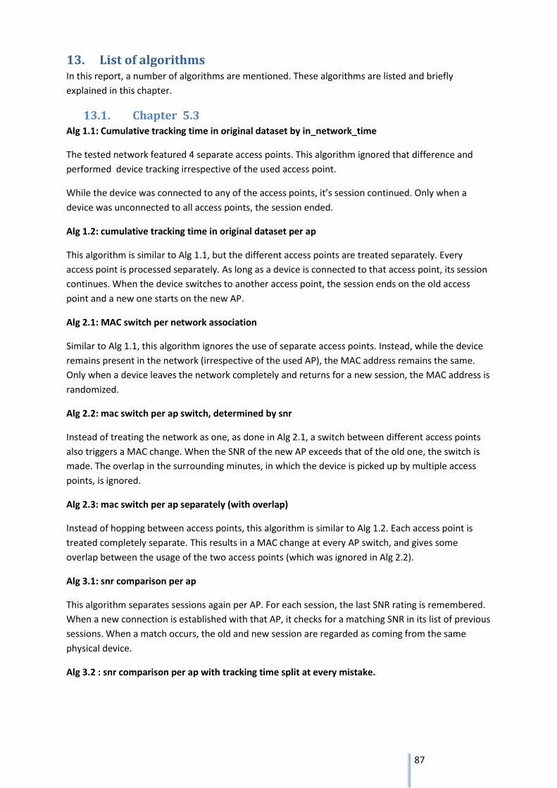
87
13. List of algorithms In this report, a number of algorithms are mentioned. These algorithms are listed and briefly
explained in this chapter.
13.1. Chapter 5.3 Alg 1.1: Cumulative tracking time in original dataset by in_network_time
The tested network featured 4 separate access points. This algorithm ignored that difference and
performed device tracking irrespective of the used access point.
While the device was connected to any of the access points, it’s session continued. Only when a
device was unconnected to all access points, the session ended.
Alg 1.2: cumulative tracking time in original dataset per ap
This algorithm is similar to Alg 1.1, but the different access points are treated separately. Every
access point is processed separately. As long as a device is connected to that access point, its session
continues. When the device switches to another access point, the session ends on the old access
point and a new one starts on the new AP.
Alg 2.1: MAC switch per network association
Similar to Alg 1.1, this algorithm ignores the use of separate access points. Instead, while the device
remains present in the network (irrespective of the used AP), the MAC address remains the same.
Only when a device leaves the network completely and returns for a new session, the MAC address is
randomized.
Alg 2.2: mac switch per ap switch, determined by snr
Instead of treating the network as one, as done in Alg 2.1, a switch between different access points
also triggers a MAC change. When the SNR of the new AP exceeds that of the old one, the switch is
made. The overlap in the surrounding minutes, in which the device is picked up by multiple access
points, is ignored.
Alg 2.3: mac switch per ap separately (with overlap)
Instead of hopping between access points, this algorithm is similar to Alg 1.2. Each access point is
treated completely separate. This results in a MAC change at every AP switch, and gives some
overlap between the usage of the two access points (which was ignored in Alg 2.2).
Alg 3.1: snr comparison per ap
This algorithm separates sessions again per AP. For each session, the last SNR rating is remembered.
When a new connection is established with that AP, it checks for a matching SNR in its list of previous
sessions. When a match occurs, the old and new session are regarded as coming from the same
physical device.
Alg 3.2 : snr comparison per ap with tracking time split at every mistake.

88
As an addition to Alg 3.1, the total tracking time isn’t calculated over all determined connections, but
only over the correct ones. At each incorrect link, the tracking time count starts again. This algorithm
better reflects the actual tracking time that was achieved. A wrong prediction shouldn’t count as real
tracking time.
Alg 3.3: snr comparison without AP separation
This algorithm is similar to Alg 3.1, only no distinction is made between access points. Final SNR
ratings are recorded for every session. A new session, on any access point is compared to all previous
sessions over all AP’s.
Alg 4.1: 10% SNR variation
Instead of using the SNR figures as recorded during the SIGCOMM conference, an offset is
determined for every session. All SNR ratings within that session are altered by that offset which is
limited to 10% of the original value.
13.2. Chapter 6 Alg 5.1: device count detection
This algorithm bases its occupancy detection on the number of active devices in the network. Per
timeslot, every device that transmits or receives any data is counted. The total per timeslot is
compared to a threshold to determine occupancy. In households without stationary devices, this
threshold is 0. When stationary devices are present, the threshold is based on the minimum
occurring device count.
Alg 5.2: packet count detection
Similar to Alg 5.1, this algorithm bases its occupancy detection on network activity. But instead of
counting devices, the total amount of data in that timeslot is counted. Without residents present, the
amount of data transmitted will usually be at its lowest point. Similar to a part of algorithm 5.1, the
prediction threshold is based on the minimum occurring data count.

89
14. Appendix I: Documentation of the initial research The initial research part covered in chapter 3 names multiple forms used in the process of this
research part. These forms are added with this Appendix. In order, this Appendix includes:
1. The informational letter send to each selected household at the beginning of the research
2. The informational brochure given to each participant
3. The blank timesheets given to each participant to fill out during the experiment

90
14.1. Informational letter
The informational letter is added after this page.

91
***For english, see other side*** Beste Medestudent, High tech inbraken op een high tech universiteit. Klinkt dat nog ver weg? De vakgroep SCS (services, cybersecurity and safety) zou graag bij jou thuis enkele metingen verrichten om te kijken in hoeverre dit een probleem in de toekomst zou kunnen zijn. Wij denken dat het toenemende gebruik van Wi-Fi de een inbreker kan vertellen wanneer u thuis bent. Om dit wetenschappelijk aan te kunnen tonen willen we graag de aanwezigheid meten bij verschillende huishoudens. De vraag aan jou is of je hierbij wil helpen. Wil je aan het begin staan van een nieuwe vorm van inbraakpreventie en daarmee een mogelijk probleem vooraf al in de kiem te smoren? Wat houdt het in? In de praktijk zou een inbreker een meetapparaat buiten de woning plaatsen. Dit apparaat vangt alle Wi-Fi signalen die door de lucht gestuurd worden op. Door bij te houden welke apparatuur op welke tijd gegevens verstuurd kan de inbreker bepalen wanneer er niemand thuis is, en dus wanneer hij het beste naar binnen kan gaan. Voor dit onderzoek vragen we je om ons meetapparaat in je huis te plaatsen. Omdat wij niet proberen te onderzoeken welk soort apparatuur het beste is voor dit soort doeleinden, maar puur of Wi-Fi signalen op deze manier te misbruiken zijn, is plaatsing binnen geen probleem. Dit voorkomt ook ingewikkelde en dure apparatuur voor de testopstelling. Bereik, stroomverbruik en dergelijke zijn namelijk een minder kritisch probleem. Voor het aantonen van het potentiële gevaar zijn de omstandigheden van minder groot belang. Ons meetapparaat slaat enkel op welk apparaat op welke tijd aanwezig is. Privacy gevoelige informatie zoals bezochte websites, wachtwoorden en dergelijke zijn voor ons niet inzichtelijk en worden ook niet opgeslagen. De data wordt voordat het wordt opgeslagen direct geanonimiseerd en na het onderzoek verwijderd. Gedurende het onderzoek van één week vragen we je om bij te houden wanneer je thuis was. Zo kunnen we vaststellen of we, aan de hand van de metingen, correct kunnen voorspellen wanneer er niemand thuis is. Als de betrouwbaarheid van deze metingen hoog is, is het voor een inbreker een potentieel interessante techniek. De tweede stap van dit onderzoek is dan ook om te gaan werken aan een aantal mogelijke oplossingen van dit probleem, voordat het misbruikt wordt. We gaan die preventieve maatregelen uitwerken en zullen de resultaten ter zijne tijd met je delen. Wat moet ik doen? Op dit moment hoef je nog niets te doen. Deze brief is enkel informatief. Binnenkort nemen we persoonlijk contact met je op om te vragen of je aan dit onderzoek mee wilt doen. Daarbij kunnen we je voorzien van extra informatie en kunnen we eventuele vragen beantwoorden. Als je besluit mee te doen plaatsen we het meetapparaat in de woning en krijg je van ons een lijst om je aanwezigheid op in te vullen. Vervolgens komen we na ongeveer één week langs om alles weer op te halen. We hopen dat je bereid bent mee te helpen, Met vriendelijke groet,
[name]
[name]
[name]

92
Dear fellow students,
High tech burglary on a high tech university, does that sound far-fetched to you? The department of services,
cybersecurity and safety is not so sure about that. Therefore we would like to perform some measurements in
your apartment to find out if this could be a problem in the future.
We think that the increasing amount of Wi-Fi usages can tell a burglar when you are home are not. To be able
to proof this risk scientifically, we want to measure this occupancy ourselves in several apartments across the
university’s campus. Our question to you is: would you like to participate in this research and be at the start of
a new type of burglary prevention? With your help, we may be able to solve this, before it becomes a problem.
How does it work? In a realistic situation, a burglar would place a measuring device outside your home. This device listens to all Wi-Fi signals it can receive and keeps track of the presence of all the devices it has found. This data can be used by a burglar to determine when nobody is at home and thus determine the best time to break in. For this research, we like to place a measuring device inside your house. If the equipment was placed outside, range, power consumption and such would be a concern. This would also drive up the price and complexity of the devices. But as this research covers the theoretical possibilities of this kind of tracking, placing the devices indoor isn’t a problem. Our measuring device only records which devices are present at what times. Privacy sensitive information like visited websites, passwords and such are not visible for us and not recorded. All data is anonymised by the measuring device before stored and it will be deleted at the end of this research. During the course of the research, which is approximately one week, we ask you to keep a log of your presence at home. We can use this log to measure if we can accurately measure the occupancy because it may be an interesting technique for a burglar to use. Therefore second part of this research concerns a number of ways to counter this problem, before people start using it. We will inform you about the progress of our work and about the countermeasures. What do I have to do? As of this moment, nothing. This letter is only informative. However, soon we will contact you personally to ask for your participation in this research. At that time we also provide extra information and answer any questions you may have. If you decide to participate, we place our measuring device (which is about the size of a wallet) at your home and provide you with a list to log your presence. After approximately one week we come by again to retrieve everything. We hope we can count on your support, Kind regards
[name]
[name]
[name]

93
14.2. Informational brochure
The informational brochure is added after this page.

94

95

96

97

98
14.3. Blank timesheets
The blank timesheets are added after this page.

99
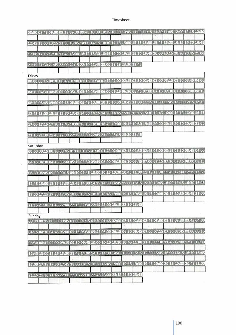
100

101
15. Appendix II: Conference data error corrections This appendix covers the classification and correction of data errors found in the 2001 SIGCOMM Wi-
Fi trace. Depending on the type of error and its location in the dataset corrections could be required.
These corrections are listed in this Appendix. The detected errors are all have to do with the
combination of MAC addresses and their Signal to noise ratios (SNR). As packet counts and such data
aren’t used in this research, errors in this data would go unnoticed.
15.1. Missing values In 20 cases, a trace missed a SNR values. For example, in one trace the list of MAC addresses counted
23 devices similar to the byte- and packet counts. The list of SNR values however, only counted 22.
These error were checked and corrected manually. The corrections are listed in Table 5 below.
Most missing values are at situated at one of the ends of a presence for that device or appear as
individual values without presence in surrounding traces. In these cases, removal of the traces has
very little influence on the data. This is also the easiest solution for the SNR attack step. When, for
example, one of the individual data points would be kept, the actual SNR value would still be
unknown. Picking a random value would have influence on the SNR comparisons. Another option
would be to pick the same value as the last known SNR of that device enabling the SNR attack to
stitch the two presences together. This is a viable technique, but has approximately the same result
as just removing the individual value. The minutes lost by removing the traces are marginal
compared to the total trace times.
In three cases, a SNR value is missing in the middle of a device presence. In all these cases the SNR
ratios are the same before and after this trace. The most likely situation is that this trace should have
Device Timestamp AP Classification
7 2964 3
Device not present in surrounding traces. Device removed from trace
12 3111 2
18 541 4
21 1822 2
52 423 4
93 1730 3
48 458 2 Missing SNR value occurs at the beginning of a presence. Device removed from trace 129 486 3
26 157
Missing SNR value lies within a device’s presence with constant SNR values. Missing value is set at the same level
37 35 4
114 56 3
144 362 3
190 350
85 2959 4
Missing SNR value occurs at the end of a presence. Device removed from trace
121 1827 1
129 1647 3
141 1539 4
164 2933 4
171 1777 1
174 492 2
Table 5: Overview of missing SNR values by classification

102
the same SNR value as its surrounding values. The alternative is removing this value, which will is the
equivalent of a device suddenly disappearing for a minute and then returning with the exact same
SNR values.
15.2. Duplicate values Some traces contain duplicate devices with, therefore, duplicated SNR values. In total these duplicate
values occur 4671 times. As choosing the right value is important for the SNR comparisons, different
solutions are chosen depending on the situation.
Most duplicates (4352) occur in the middle of a device’s presence. As SNR comparison only happens
at the beginning and end values of a presence, these ‘middle’ values are of no importance for this
research. In 3382 cases, one of the duplicate values matched the SNR values of surrounding traces. In
these cases, this matching value is chosen. In other cases, just one of the values is picked.
In 234 cases, the duplicate SNR value is 0. In these cases, the nonzero value is chosen.
The remaining 85 duplicates are compared to the earlier and later presences to check for SNR
matches. In case of a duplicate at the beginning of a presence, if one of the duplicates match the last
SNR of the previous presence this value is chosen. This enables SNR comparison. If both values don’t
match, the SNR comparison will not work. The chosen value doesn’t matter in this case. This gave the
following distribution:
38x no matching values to previous presence
38x no matching values to next presence
5x SNR match with previous presence
2x No previous presences available, any value will do
This leaves 2 remaining duplicates. These were checked manually.
Device 26 timestamp 156 had duplicates of 37 and 38. This last value matches the surrounding values but due to a missing SNR at timestamp 157 this wasn’t picked up in earlier steps.
Device 190 timestamp 350 had duplicates of 34 and 30. Similar to the previous duplicate a match wasn’t made due to a missing value in the next trace. Value set to 30, matching the surrounding SNR value.
15.3. Unrealisitic values The representation and value range of Signal to noise ratios differ from manufacturer to
manufacturer. In this case, almost all values seem to lie below 75. Some traces, however, feature
very high SNR values:
236 (2x)
2925 (13x)
5192 (1x)
6912 (3x)
6916 (1x)
9217 (1x)

103
These values are likely to be errors, but their strange values don’t have to be changed as their
influence is limited. The single high values may prevent a SNR match, but changing the value to
achieve this match without proper reasoning will influence the results. And in the case of SNR value
2925. The 13 occurences are mostly concentrated in 1 presence and a couple in a separate ones
around it. Although the value is strange, a SNR comparison can still be performed here.
15.4. SNR values of zero Device 194 never features SNR values other than zero. This device only occurs once in the complete
trace for 4 minutes. As this device hasn’t got much influence on the trace, the choice was made to
remove it. Alternatively it could’ve gotten a SNR trace that would mismatch all other devices to
prevent wrong SNR comparisons. But the results of this are almost the same. In the first trace, this
yields one extra trace of 4 minutes which is marginal.
15.5. Conclusion The dataset contained almost 5000 errors which were corrected in different ways. Although most
corrections are small in comparison to the dataset, together they could induce small differences
between the results of this and the previous research.
104
16. Appendix III, Household modeling and tracking
16.1. Introduction This model is designed to test the effect of MAC randomisation under different household configurations. Real world tests would demand enormous amounts of time and effort to get a modest amount of datasets. Instead this script generates households with their traffic patterns to test the mac randomisation hypothesis.
16.2. Used data and limitations
16.2.1. Networking devices
In this model, households are created with some networking devices. Depending on the residents’
schedule(s), these devices generate a network trace. For this part, different networking devices were
traced under known circumstances. This created realistic traces to be used for this model.
Numerous types of devices can be found in the modern household. Due to time and availability
restrictions, not all possible devices have been traced. Also, of each device, only 1 trace was created.
In real life, different brands and types would create different patterns. The usability of this model to
represent the real world is therefore very limited. However, as the goal for this research part is to
show the theoretical usability of MAC randomisation, a limited model is enough at this point. Should
the proposal turn out to be promising, a more elaborate model should be created.
For this research, the following devices have been traced: Smart TV: Smart TV’s emerged in the last couple of years. It integrates multimedia functionality like youtube,
Netflix, internet browsing and others into a normal television. This also means it’s connected to a
network. It’s obvious that watching a youtube video generates a lot of network traffic, but with
features like voice control generously send out data to online voice recognition servers [27].

105
A network trace of a Philips 40PFK5500/12 smart tv resulted in the following data pattern:
Figure 50: Visualised network trace of a Philips 40PFK5500/12 smart TV
In the first 15 minutes, it displayed normal cable tv. The trace shows that even without actively using
the network as a user, the tv is constantly generating traffic. After 15 minutes the tv is switched to
youtube (3 consecutive videos) and after 28 minutes to an IPTV stream. Both services generate large
amounts of data as would be expected. After approximately 45 minutes the tv is turned off
(standby). Obviously the large amount of traffic from the videos falls away, but the tv keeps
generating traffic. The zoomed in trace of Figure 51 shows that even in standby, the TV generates
around 26 packets a minute.
Figure 51: Part of the visualised network trace of a Philips 40PFK5500/12 smart TV

106
Smart thermostat Nowadays, more and more household devices are network connected. One of these devices is the central heating controller. In addition to the temperature control we have known for years it enables us to connect it to our smartphones and enrol advanced heating scheme’s based on our life patterns, adjust current temperature without even getting up from the couch and easily monitor our energy usage. A trace of a household with a Nefit Easy thermostat yielded the results of Figure 52 below:
Figure 52: Visualised network trace of a Nefit Nest smart thermostat
Just as a lot of other devices it creates a nice and constant stream of traffic of around 8 packets per minute with a reasonably constant packet size distribution. In addition to this, some large packets are generated exactly every 15 minutes. These kind of patterns could be very helpful for a burglar snooping the household’s traffic. Smartphone The smartphone is the most important device for a lot of people, but also for a burglar. As people generally carry it with them all day long, it serves as a big indicator for someone’s presence. For this research, a Sony Xperia Z5 compact running Android 7.0 was tested. The trace of this phone can be divided in 2 parts. In part one, the phone was used as normal for approximately 1.5 hours, with some web browsing, whatsapp, video streaming and idle moments.

107
Figure 53: Visualised network trace of a Sony Xperia Z5 compact smartphone running Android 7.0
Secondly, a trace was made at night to capture the behaviour when the phone isn’t used for a long time. The device falls into deep sleep with little activity and network traffic.
Figure 54: Visualised network trace of a Sony Xperia Z5 compact smartphone running android 7.0 in standby during sleep hours
Network printer One of the network printers tested was a Hewlett Packard Photosmart 4700 series. As printing jobs
are usually rare, irregular and only occur when a resident is at home this part isn’t tested. The idle
behaviour of the system is the most important in this situation as it has to mask absent users.
The network trace of the network printer is visualised in Figure 55 below with a boxplot on the
average packet size per minute and a line plot on the packet count.

108
Figure 55:Visualised network trace of a Hewlett Packard Photosmart C4780 network printer
The first 13 minutes shown high network activity. At this time the main computer was still active. As
this computer has the full software suite installed it isn’t unlikely that the printer keeps contact with
this computer to check for software updates and other functionality. At approximately 21 minutes,
all residents leave the house. After this time the printer generates a recurring pattern with a activity
spike every 60 minutes. When the printer is shut down completely instead of left in standby (soft off
as there is no physical power switch), the traffic generation stops completely.
In general the printer will generate a relatively constant stream of data, but the amount is very low.
With only a printer in the network presence of other devices like smartphones could be easily
detected. Also, the recurring data pattern could enable someone to combine different MAC
addresses together again.
16.2.2. Household statistics
Fully randomized datasets won’t give a very realistic representation of real world households. Instead, the model is based on some statistics of Dutch households. The major sources for statistics were:
Statistics Netherlands (CBS) via their open CBS statline data portal
Royal Dutch science academy (KNAW) via the data archiving and networked services (DANS) portal
Some used data tables from the Statline portal are:
Occurrence of households by size and composition (2016) [A]
Distribution of residents across household types (2016) [C]
Age distributions of residents per household type (2016) [E]
Age difference of partner in married couples (2015) [F]
Distribution of working hours per week by age group (2016) [B]
Distribution of time across activities by age group (2011) [D] Other data was obtained from: KNAW DANS portal:

109
A research into activities of Dutch citizens [H]. This research formed the basis for the Statline activities distribution [D].
Stichting kijkonderzoek (SKO):
A research into the occurrence of different devices across Dutch households (2017)[G]
16.2.3. Limitations
Due to limitations in gathered data, limited time and other factors, some limitations are given to the
created model.
Devices and network traces:
As stated earlier, due to time and availability limitations, only 1 device of every type was traced. This gives the generated data traces a bias for certain patterns. In real life, generated network patters could be much more divers.
Network traces only cover a limited amount of time. In the model, a trace of 1 week is created. Depending on the required trace length for that device, multiple instances of the created trace have been inserted after each other. This could give some extra patterns.
In the end, some datasets weren’t used in the model, or only limited: o Smart TV:
To keep the model manageable, only the network trace of a smart tv on cable is used. Statistics into the distribution between cable, IPTV and such are limited and implementing these adds a lot of difficulty to the model.
o IP cam Due to missing statistics on the occurrence and usage of IP cameras. This device
was left out of the model.
Statistics/model:
Most statistics were divided into age blocks of 5 years. These blocks are also used in the model.
Due to missing statistics on daily activities, the presence of residents below 15 years old isn’t taken into account. It is assumed that most of them would follow a similar schedule to one of the parents. Giving them a separate trace would therefore give very unrealistic patterns or barely any difference against a similar household with the child left out.
In the models, no distinction is made between male and female residents. Although some statistics do have this distinction, a lot of them don’t. The differences between these groups are also limited in most cases and would complicate the model further.
Networking devices are considered to be connected to a wireless network. In reality, a portion of smart TV’s, laptops and other devices would be connected via a wired interface and therefore won’t show up in the wireless trace. As households are also created without (networked) TV’s and computers, this effect is already created.
Stationary devices like a network printer and smart thermostat are considered to be connected continuously.
Time apart from sleeping and working is divided in “activity blocks” of 30-240 minutes. The activity performed in this time block is then determined by chance based on the statistics of [D].
A resident has a high chance of owning a smartphone as is the case in real life. When the resident owns one, he/she is assumed to always carry the phone with them and have its WiFi turned on.
The model doesn’t include more complicated scenarios like: o Forgetting to turn a device on or off

110
o Disabling the network at certain times o Visitors o Changes in available devices during the trace o Multiple of the same devices per household (excluding smartphones) and the
division of active time across them
16.3. Matlab household model: The matlab household creation model is divided into different functions. Each part is explained shortly in this section.
1. Household creation This script determines the type of household (single person, single parent with 2 children etc) and the age group of all residents. Some of the statistics listed earlier are used for this. The script returns a data structure with all relevant information.
2. Device creation This script determines for each resident in the given household if they have a smartphone and for the complete house if there is a TV (no, standard, smart, chromecast), network printer, tablet, thermostat, etc.
3. Activity creation This script determines for each of the residents if they have a job and, if so, which days and hours they work. After this step, their sleep time is determined based on available statistics. The remaining time blocks are listed, divided in segments of 30-240 minutes and get an activity assigned to them by chance. The probabilities for each activity to occur are based on statistics.
4. Schedule creation This script takes the activity schedule of all residents and translates them into device schedules. When 2 activities overlap they are joined together. For example, when resident 1 watches TV from minute 0 to 100 and resident 2 from 80 to 150, they are combined into 1 activity for the TV from 0 to 150.
5. Trace creation This script generates the actual traces of each device in the household based on the activities from the schedule creator. The smarthone trace is empty when a resident is away from home, active when a resident is at home and not sleeping and in standby mode when the resident is sleeping. When residents are watching TV on a smart TV, it is determined to be cable TV. When the household has a network printer or smart thermostat, a 7 days continuous trace is generated and added to the household. All traces are divided into 1 minute blocks with packet counts per payload size to keep the data size manageable.
6. Trace randomisation To simulate the implementation of a MAC randomisation scheme, all device traces are divided into blocks with a random length between 3 and 15 minutes. The switched addresses are considered to be unlinkable.
16.4. Matlab data processors After creating households, an automated trace processor is used to try and extract the vital
occupancy information a burglar would be searching for. With the MAC randomization system, this
information should at least become less reliable. The used data processors are described in chapter
6.4 with their results.

111
16.5. References [A] http://statline.cbs.nl/Statweb/publication/?VW=T&DM=SLNL&PA=82905NED&D1=31-
50&D2=0,5,10,15,20-22&HD=171012-1104&HDR=T&STB=G1 [B] http://statline.cbs.nl/Statweb/publication/?VW=T&DM=SLNL&PA=82309NED&D1=0-2,11-
23&D2=0&D3=11-22&D4=0&D5=69&HD=171012-1106&HDR=G4&STB=G1,G2,G3,T [C] http://statline.cbs.nl/Statweb/publication/?VW=T&DM=SLNL&PA=82905NED&D1=a&D2=
0,5,10,15,20-22&HD=171012-1110&HDR=T&STB=G1 [D] http://statline.cbs.nl/Statweb/publication/?VW=T&DM=SLNL&PA=82617NED&D1=0-
20&D2=0-9&D3=l&HD=171012-1114&HDR=T&STB=G2,G1 [E] http://statline.cbs.nl/Statweb/publication/?VW=T&DM=SLNL&PA=37620&D1=a&D2=0&D3
=0,97-116&D4=21&HD=171012-1115&HDR=T&STB=G1,G2,G3 [F] http://statline.cbs.nl/Statweb/publication/?VW=T&DM=SLNL&PA=60036NED&D1=4-
16,235&D2=l&HD=171012-1119&HDR=G1&STB=T [G] https://kijkonderzoek.nl/images/Persberichten_algemeen/170720_Persbericht_TV_in_
Nederland_1e_helft_2017.pdf [H] Met het oog op de tijd. Een blik op de tijdsbesteding van Nederlanders:
https://easy.dans.knaw.nl/ui/datasets/id/easy-dataset:57866/tab/1

112
17. Appendix IV: Report of prior literature research
A copy of the literature research preformed before the start of this thesis is added after this page.