HOL-TestGen: User Guide - Achim D. Brucker
120
LRI Technical Report 1551 HOL-TestGen 1.7.0 User Guide http://www.brucker.ch/projects/hol-testgen/ Achim D. Brucker [email protected] SAP AG, SAP Research, Karlsruhe, Germany Lukas Br¨ ugger [email protected] ETH, Z¨ urich, Switzerland Matthias P. Krieger [email protected] LRI, Orsay, France Burkhart Wolff wolff@lri.fr LRI, Orsay, France November 5, 2012 Laboratoire en Recherche en Infromatique (LRI) Universit´ e Paris-Sud 11 91405 Orsay Cedex France
Transcript of HOL-TestGen: User Guide - Achim D. Brucker
LRI Technical Report 1551
HOL-TestGen 1.7.0User Guide
http://www.brucker.ch/projects/hol-testgen/
Achim D. [email protected]
SAP AG, SAP Research, Karlsruhe, Germany
Lukas [email protected]
ETH, Zurich, Switzerland
Matthias P. [email protected]
LRI, Orsay, France
Burkhart [email protected]
LRI, Orsay, France
November 5, 2012
Laboratoire en Recherche en Infromatique (LRI)Universite Paris-Sud 11
91405 Orsay CedexFrance

Copyright c© 2003–2012 ETH Zurich, SwitzerlandCopyright c© 2007–2012 Achim D. Brucker, GermanyCopyright c© 2008–2012 University Paris-Sud, France
Permission is granted to make and distribute verbatim copies of this manual providedthe copyright notice and this permission notice are preserved on all copies.Permission is granted to copy and distribute modified versions of this manual underthe conditions for verbatim copying, provided that the entire resulting derived work isdistributed under the terms of a permission notice identical to this one.Permission is granted to copy and distribute translations of this manual into anotherlanguage, under the above conditions for modified versions, except that this permissionnotice may be stated in a translation approved by the Free Software Foundation.
Note:This manual describes HOL-TestGen version 1.7.0 (rev. 9482).
Contents
1. Introduction 5
2. Preliminary Notes on Isabelle/HOL 72.1. Higher-order logic — HOL . . . . . . . . . . . . . . . . . . . . . . . . . . . 72.2. Isabelle . . . . . . . . . . . . . . . . . . . . . . . . . . . . . . . . . . . . . 7
3. Installation 93.1. Prerequisites . . . . . . . . . . . . . . . . . . . . . . . . . . . . . . . . . . 93.2. Installing HOL-TestGen . . . . . . . . . . . . . . . . . . . . . . . . . . . . 93.3. Starting HOL-TestGen . . . . . . . . . . . . . . . . . . . . . . . . . . . . . 10
4. Using HOL-TestGen 134.1. HOL-TestGen: An Overview . . . . . . . . . . . . . . . . . . . . . . . . . 134.2. Test Case and Test Data Generation . . . . . . . . . . . . . . . . . . . . . 134.3. Test Execution and Result Verification . . . . . . . . . . . . . . . . . . . . 19
4.3.1. Testing an SML-Implementation . . . . . . . . . . . . . . . . . . . 194.3.2. Testing Non-SML Implementations . . . . . . . . . . . . . . . . . . 21
4.4. Profiling Test Generation . . . . . . . . . . . . . . . . . . . . . . . . . . . 22
5. Core Libraries 235.1. Monads . . . . . . . . . . . . . . . . . . . . . . . . . . . . . . . . . . . . . 23
5.1.1. General Framework for Monad-based Sequence-Test . . . . . . . . 235.1.2. Valid Test Sequences in the State Exception Monad . . . . . . . . 295.1.3. Valid Test Sequences in the State Exception Backtrack Monad . . 33
5.2. Observers . . . . . . . . . . . . . . . . . . . . . . . . . . . . . . . . . . . . 335.2.1. IO-stepping Function Transfomers . . . . . . . . . . . . . . . . . . 33
5.3. Automata . . . . . . . . . . . . . . . . . . . . . . . . . . . . . . . . . . . . 375.3.1. Rich Traces and its Derivatives . . . . . . . . . . . . . . . . . . . . 395.3.2. Extensions: Automata with Explicit Final States . . . . . . . . . . 41
5.4. TestRefinements . . . . . . . . . . . . . . . . . . . . . . . . . . . . . . . . 425.4.1. Conversions Between Programs and Specifications . . . . . . . . . 42
6. Examples 476.1. Max . . . . . . . . . . . . . . . . . . . . . . . . . . . . . . . . . . . . . . . 476.2. Triangle . . . . . . . . . . . . . . . . . . . . . . . . . . . . . . . . . . . . . 49
6.2.1. The Standard Workflow . . . . . . . . . . . . . . . . . . . . . . . . 506.2.2. The Modified Workflow: Using Abstract Test Data . . . . . . . . . 52
3
6.3. Lists . . . . . . . . . . . . . . . . . . . . . . . . . . . . . . . . . . . . . . . 566.3.1. A Quick Walk Through . . . . . . . . . . . . . . . . . . . . . . . . 566.3.2. Test and Verification . . . . . . . . . . . . . . . . . . . . . . . . . . 63
6.4. AVL . . . . . . . . . . . . . . . . . . . . . . . . . . . . . . . . . . . . . . . 696.5. RBT . . . . . . . . . . . . . . . . . . . . . . . . . . . . . . . . . . . . . . . 73
6.5.1. Advanced Elements of the Test Specification and Test-Case-Generation 786.5.2. Standard Unit-Testing of Red-Black-Trees . . . . . . . . . . . . . . 796.5.3. Test Data Generation . . . . . . . . . . . . . . . . . . . . . . . . . 806.5.4. Configuring the Code Generator . . . . . . . . . . . . . . . . . . . 846.5.5. Test Result Verification . . . . . . . . . . . . . . . . . . . . . . . . 846.5.6. Test Data Generation . . . . . . . . . . . . . . . . . . . . . . . . . 87
6.6. Sequence Testing . . . . . . . . . . . . . . . . . . . . . . . . . . . . . . . . 886.6.1. Reactive Sequence Testing . . . . . . . . . . . . . . . . . . . . . . . 886.6.2. Basic Technique: Events with explicit variables . . . . . . . . . . . 896.6.3. The infrastructure of the observer: substitute and rebind . . . . . 896.6.4. Abstract Protocols and Abstract Stimulation Sequences . . . . . . 906.6.5. The Post-Condition . . . . . . . . . . . . . . . . . . . . . . . . . . 916.6.6. Testing for successful system runs of the server under test . . . . . 916.6.7. Test-Generation: The Standard Approach . . . . . . . . . . . . . . 916.6.8. Test-Generation: Refined Approach involving TP . . . . . . . . . . 926.6.9. Deterministic Bank Example . . . . . . . . . . . . . . . . . . . . . 946.6.10. Non-Deterministic Bank Example . . . . . . . . . . . . . . . . . . 100
A. Glossary 105
4
1. Introduction
Today, essentially two validation techniques for software are used: software verificationand software testing . Whereas verification is rarely used in “real” software develop-ment, testing is widely-used, but normally in an ad-hoc manner. Therefore, the attitudetowards testing has been predominantly negative in the formal methods community,following what we call Dijkstra’s verdict [19, p.6]:
“Program testing can be used to show the presence of bugs, but never toshow their absence!”
More recently, three research areas, albeit driven by different motivations, converge andresult in a renewed interest in testing techniques:
Abstraction Techniques: model-checking raised interest in techniques to abstract in-finite to finite models. Provided that the abstraction has been proven sound,testing may be sufficient for establishing correctness [10, 18].
Systematic Testing: the discussion over test adequacy criteria [27], i. e. criteria solvingthe question “when did we test enough to meet a given test hypothesis,” led tomore systematic approaches for partitioning the space of possible test data andthe choice of representatives. New systematic testing methods and abstractiontechniques can be found in [22, 20].
Specification Animation: constructing counter-examples has raised interest also inthe theorem proving community, since combined with animations of evaluations,they may help to find modeling errors early and to increase the overall productiv-ity [9, 23, 17].
The first two areas are motivated by the question “are we building the program right?”the latter is focused on the question “are we specifying the right program?” Whilethe first area shows that Dijkstra’s Verdict is no longer true under all circumstances,the latter area shows, that it simply does not apply in practically important situations.In particular, if a formal model of the environment of a software system (e. g. basedamong others on the operation system, middleware or external libraries) must be reverse-engineered, testing (“experimenting”) is without alternative (see [12]).
Following standard terminology [27], our approach is a specification-based unit test .In general, a test procedure for such an approach can be divided into:
Test Case Generation: for each operation the pre/postcondition relation is dividedinto sub-relations. It assumes that all members of a sub-relation lead to a similarbehavior of the implementation.
5

Test Data Generation: (also: Test Data Selection) for each test case (at least) onerepresentative is chosen so that coverage of all test cases is achieved. From theresulting test data, test input data processable by the implementation is extracted.
Test Execution: the implementation is run with the selected test input data in orderto determine the test output data.
Test Result Verification: the pair of input/output data is checked against the spec-ification of the test case.
The development of HOL-TestGen [14] has been inspired by [21], which follows the lineof specification animation works. In contrast, we see our contribution in the developmentof techniques mostly on the first and to a minor extent on the second phase. Building onQuickCheck [17], the work presented in [21] performs essentially random test, potentiallyimproved by hand-programmed external test data generators. Nevertheless, this workalso inspired the development of a random testing tool for Isabelle [9]. It is well-knownthat random test can be ineffective in many cases; in particular, if preconditions of aprogram based on recursive predicates like “input tree must be balanced” or “inputmust be a typable abstract syntax tree” rule out most of randomly generated data.HOL-TestGen exploits these predicates and other specification data in order to produceadequate data. As a particular feature, the automated deduction-based process can logthe underlying test hypothesis made during the test; provided that the test hypothesis isvalid for the program and provided the program passes the test successfully, the programmust guarantee correctness with respect to the test specification, see [11, 15] for details.
6
2. Preliminary Notes on Isabelle/HOL
2.1. Higher-order logic — HOL
Higher-order logic(HOL) [16, 8] is a classical logic with equality enriched by total poly-morphic1 higher-order functions. It is more expressive than first-order logic, since e. g.induction schemes can be expressed inside the logic. Pragmatically, HOL can be viewedas a combination of a typed functional programming language like Standard ML (SML)or Haskell extended by logical quantifiers. Thus, it often allows a very natural way ofspecification.
2.2. Isabelle
Isabelle [24, 2] is a generic theorem prover. New object logics can be introduced byspecifying their syntax and inference rules. Among other logics, Isabelle supports firstorder logic (constructive and classical), Zermelo-Frankel set theory and HOL, which wechose as the basis for the development of HOL-TestGen.
Isabelle consists of a logical engine encapsulated in an abstract data type thm inStandard ML; any thm object has been constructed by trusted elementary rules inthe kernel. Thus Isabelle supports user-programmable extensions in a logically safeway. A number of generic proof procedures (tactics) have been developed; namely asimplifier based on higher-order rewriting and proof-search procedures based on higher-order resolution.
We use the possibility to build on top of the logical core engine own programs per-forming symbolic computations over formulae in a logically safe (conservative) way: thisis what HOL-TestGen technically is.
1to be more specific: parametric polymorphism
7

3. Installation
3.1. Prerequisites
HOL-TestGen is build on top of Isabelle/HOL, version 2011-1, thus you need a workinginstallation of Isabelle 2011-1. To install Isabelle, follow the instructions on the Isabelleweb-site:
http://isabelle.in.tum.de/website-Isabelle2011-1/index.html
If you use the pre-compiled binaries from this website, please ensure that you installboth the Pure heap and HOL heap.
3.2. Installing HOL-TestGen
In the following we assume that you have a running Isabelle 2009 environment includ-ing the Proof General based front-end. The installation of HOL-TestGen requires thefollowing steps:
1. Unpack the HOL-TestGen distribution, e. g.:
tar zxvf hol-testgen-1.7.0.tar.gz
This will create a directory hol-testgen-1.7.0 containing the HOL-TestGen dis-tribution.
2. Check the settings in the configuration file hol-testgen-1.7.0/make.config. Ifyou can use the isabelle tool from Isabelle on the command line to start Isabelle2011-1, the default settings should work. The ISABELLE variable in textttmake.configneeds to point to the 2011-1 version of Isabelle. For this, it can be necessary toconfigure an absolute path, e.g.,
ISABELLE=/usr/local/Isabelle2011-1/bin/isabelle
3. Change into the src directory
cd hol-testgen-1.7.0/src
and build the HOL-TestGen heap image for Isabelle by calling
isabelle make
9
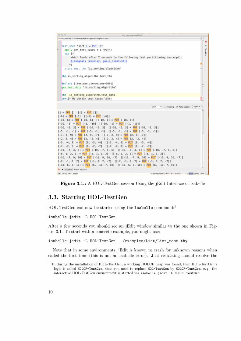
Figure 3.1.: A HOL-TestGen session Using the jEdit Interface of Isabelle
3.3. Starting HOL-TestGen
HOL-TestGen can now be started using the isabelle command:1
isabelle jedit -L HOl-TestGen
After a few seconds you should see an jEdit window similar to the one shown in Fig-ure 3.1. To start with a concrete example, you might use:
isabelle jedit -L HOL-TestGen ../examples/List/List_test.thy
Note that in some environments, jEdit is known to crash for unknown reasons whencalled the first time (this is not an Isabelle error). Just restarting should resolve the
1If, during the installation of HOL-TestGen, a working HOLCF heap was found, then HOL-TestGen’slogic is called HOLCF-TestGen; thus you need to replace HOL-TestGen by HOLCF-TestGen, e. g. theinteractive HOL-TestGen environment is started via isabelle jedit -L HOLCF-TestGen.
10
problem. In general, we strongly recommend to use the jEdit client as user-interface(instead of Proof General).2 Use the system manual (see http://isabelle.in.tum.de/website-Isabelle2011-1/dist/Isabelle2011-1/doc/system.pdf) as a high-level de-scription of jEdit’s system options; another source of information is the built-in README-facility inside the jEdit client.
2Still, in case you are using an non re-parenting window manager, you might want to stick to ProofGeneral as jEdit has some problems with such window managers.
11

4. Using HOL-TestGen
4.1. HOL-TestGen: An Overview
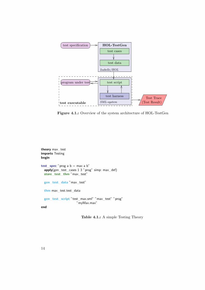
HOL-TestGen allows one to automate the interactive development of test cases, refinethem to concrete test data, and generate a test script that can be used for test executionand test result verification. The test case generation and test data generation (selection)is done in an Isar-based [26] environment (see Figure 4.1 for details). The Test executable(and the generated test script) can be build with any SML-system.
4.2. Test Case and Test Data Generation
In this section we give a brief overview of HOL-TestGen related extension of the Isar [26]proof language. We use a presentation similar to the one in the Isar Reference Man-ual [26], e. g. “missing” non-terminals of our syntax diagrams are defined in [26]. Weintroduce the HOL-TestGen syntax by a (very small) running example: assume we wantto test a functions that computes the maximum of two integers.
Starting your own theory for testing: For using HOL-TestGen you have to buildyour Isabelle theories (i. e. test specifications) on top of the theory Testing insteadof Main. A sample theory is shown in Table 4.1.
Defining a test specification: Test specifications are defined similar to theorems inIsabelle, e. g.,
test spec ”prog a b = max a b”
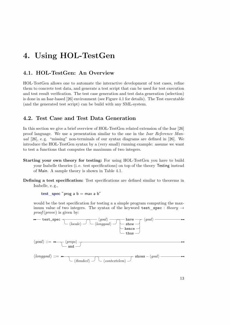
would be the test specification for testing a a simple program computing the max-imum value of two integers. The syntax of the keyword test spec : theory →proof (prove) is given by:
-- test_spec �� 〈locale〉 ��� 〈goal〉� 〈longgoal〉 ��� have� show �� hence �� thus �� 〈goal〉 -�
〈goal〉 ::=-- �〈props〉� and �� -�
〈longgoal〉 ::=-- �� 〈thmdecl〉 ���� 〈contextelem〉 �� shows 〈goal〉 -�
13
test data
test cases
program under test
test harness
test script
test specification
(Test Result)Test Trace
HOL-TestGen
Isabelle/HOL
SML-systemtest executable
Figure 4.1.: Overview of the system architecture of HOL-TestGen
theory max testimports Testingbegin
test spec ”prog a b = max a b”apply(gen test cases 1 3 ”prog” simp: max def)store test thm ”max test”
gen test data ”max test”
thm max test.test data
gen test script ”test max.sml” ”max test” ”prog””myMax.max”
end
Table 4.1.: A simple Testing Theory
14
Please look into the Isar Reference Manual [26] for the remaining details, e. g. adescription of 〈contextelem〉.
Generating symbolic test cases: Now, abstract test cases for our test specificationcan (automatically) be generated, e. g. by issuing
apply(gen test cases ”prog” simp: max def)
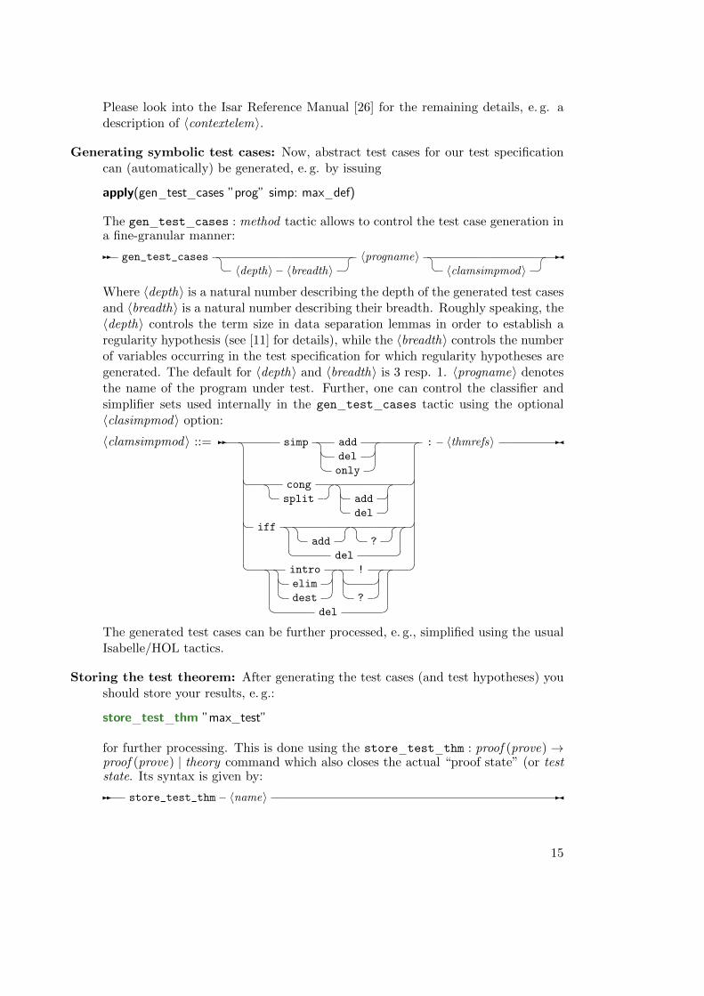
The gen test cases : method tactic allows to control the test case generation ina fine-granular manner:
-- gen_test_cases �� 〈depth〉 〈breadth〉 �� 〈progname〉 �� 〈clamsimpmod〉 ��-�Where 〈depth〉 is a natural number describing the depth of the generated test casesand 〈breadth〉 is a natural number describing their breadth. Roughly speaking, the〈depth〉 controls the term size in data separation lemmas in order to establish aregularity hypothesis (see [11] for details), while the 〈breadth〉 controls the numberof variables occurring in the test specification for which regularity hypotheses aregenerated. The default for 〈depth〉 and 〈breadth〉 is 3 resp. 1. 〈progname〉 denotesthe name of the program under test. Further, one can control the classifier andsimplifier sets used internally in the gen test cases tactic using the optional〈clasimpmod〉 option:
〈clamsimpmod〉 ::=-- � simp � add� del �� only ��
� � cong� split ���� add �� del �� �
� iff ��� add ���� ? ��� del �� �
� �� intro� elim �� dest ��� !� �� ? �
�� del �
� �
� : 〈thmrefs〉 -�
The generated test cases can be further processed, e. g., simplified using the usualIsabelle/HOL tactics.
Storing the test theorem: After generating the test cases (and test hypotheses) youshould store your results, e. g.:
store test thm ”max test”
for further processing. This is done using the store test thm : proof (prove)→proof (prove) | theory command which also closes the actual “proof state” (or teststate. Its syntax is given by:
-- store_test_thm 〈name〉 -�
15
Where 〈name〉 is a fresh identifier which is later used to refer to this test state. Is-abelle/HOL can access the corresponding test theorem using the identifier 〈name〉.test thm,e. g.:
thm max test.test thm
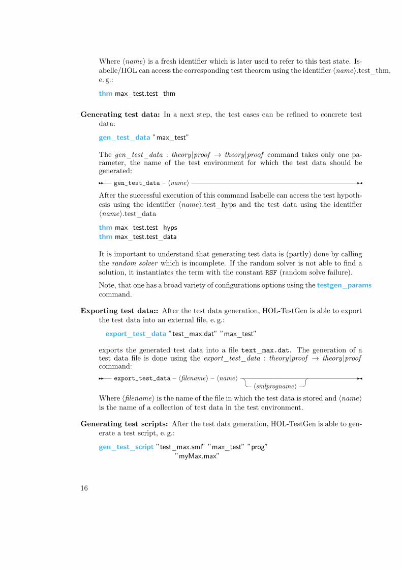
Generating test data: In a next step, the test cases can be refined to concrete testdata:
gen test data ”max test”
The gen test data : theory |proof → theory |proof command takes only one pa-rameter, the name of the test environment for which the test data should begenerated:
-- gen_test_data 〈name〉 -�
After the successful execution of this command Isabelle can access the test hypoth-esis using the identifier 〈name〉.test hyps and the test data using the identifier〈name〉.test data
thm max test.test hypsthm max test.test data
It is important to understand that generating test data is (partly) done by callingthe random solver which is incomplete. If the random solver is not able to find asolution, it instantiates the term with the constant RSF (random solve failure).
Note, that one has a broad variety of configurations options using the testgen paramscommand.
Exporting test data:: After the test data generation, HOL-TestGen is able to exportthe test data into an external file, e. g.:
export test data ”test max.dat” ”max test”
exports the generated test data into a file text max.dat. The generation of atest data file is done using the export test data : theory |proof → theory |proofcommand:
-- export_test_data 〈filename〉 〈name〉 �� 〈smlprogname〉 �� -�
Where 〈filename〉 is the name of the file in which the test data is stored and 〈name〉is the name of a collection of test data in the test environment.
Generating test scripts: After the test data generation, HOL-TestGen is able to gen-erate a test script, e. g.:
gen test script ”test max.sml” ”max test” ”prog””myMax.max”
16

structure TestDriver : sig end = struct
val return = ref ~63;
3 fun eval x2 x1 = let
val ret = myMax.max x2 x1
in
(( return := ret);ret)
end
8 fun retval () = SOME(! return );
fun toString a = Int.toString a;
val testres = [];
val pre_0 = [];
13 val post_0 = fn () => ( (eval ~23 69 = 69));
val res_0 = TestHarness.check retval pre_0 post_0;
val testres = testres@[res_0];
val pre_1 = [];
18 val post_1 = fn () => ( (eval ~11 ~15 = ~11));
val res_1 = TestHarness.check retval pre_1 post_1;
val testres = testres@[res_1];
val _ = TestHarness.printList toString testres;
23 end
Table 4.2.: Test Script
produces the test script shown in Table 4.2 that (together with the provided testharness) can be used to test real implementations. The generation of test scriptsis done using the generate test script : theory |proof → theory |proof command:
-- gen_test_script 〈filename〉 〈name〉 〈progname〉 �� 〈smlprogname〉 �� -�
Where 〈filename〉 is the name of the file in which the test script is stored, and〈name〉 is the name of a collection of test data in the test environment, and〈progname〉 the name of the program under test. The optional parameter 〈smlprogname〉allows for the configuration of different names of the program under test that isused within the test script for calling the implementation.
Configure HOL-TestGen: The overall behavior of test data and test script generationcan be configured, e. g.
testgen params [iterations=15]
using the testgen params : theory → theory command:
17
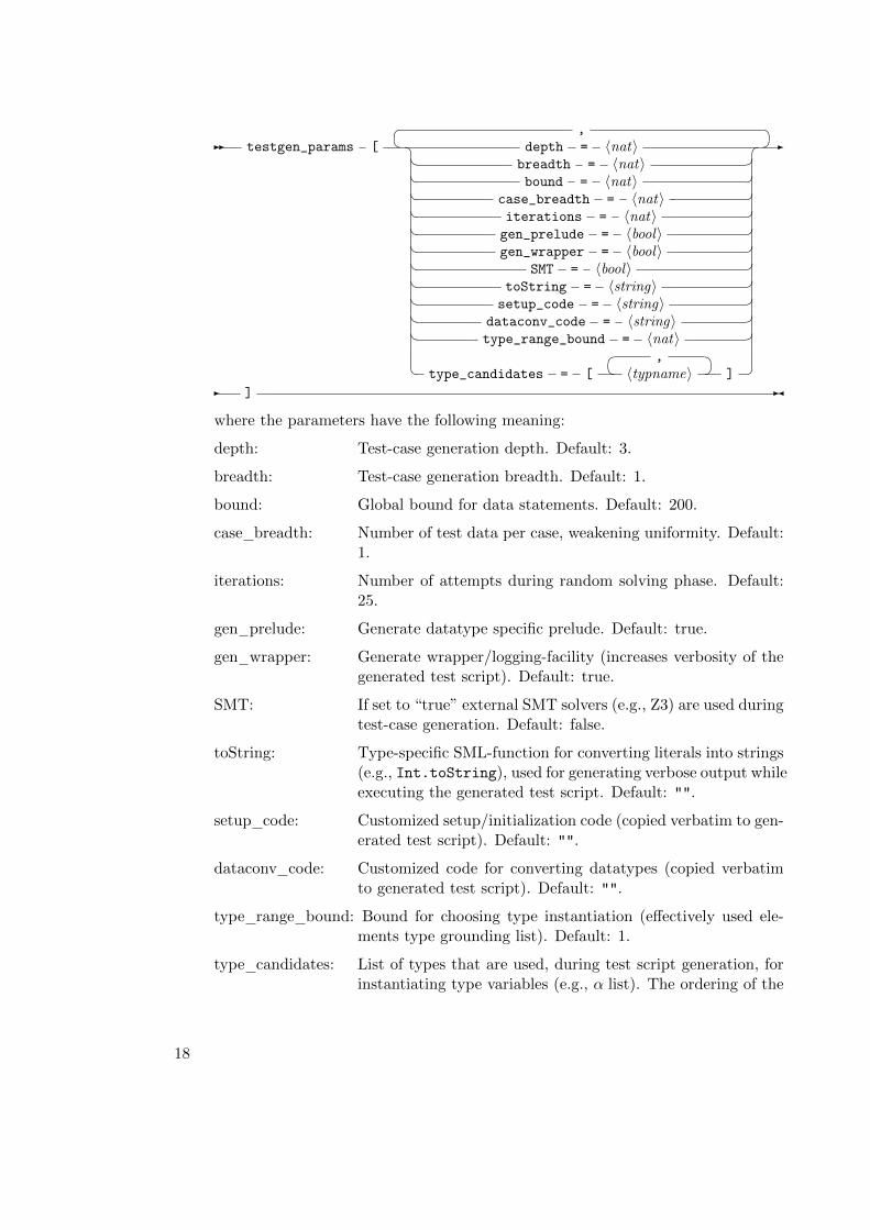
-- testgen_params [
� , �� � depth = 〈nat〉� breadth = 〈nat〉 �� bound = 〈nat〉 �� case_breadth = 〈nat〉 �� iterations = 〈nat〉 �� gen_prelude = 〈bool〉 �� gen_wrapper = 〈bool〉 �� SMT = 〈bool〉 �� toString = 〈string〉 �� setup_code = 〈string〉 �� dataconv_code = 〈string〉 �� type_range_bound = 〈nat〉 �� type_candidates = [
� , �� 〈typname〉 � ] �
� �-
- ] -�
where the parameters have the following meaning:
depth: Test-case generation depth. Default: 3.
breadth: Test-case generation breadth. Default: 1.
bound: Global bound for data statements. Default: 200.
case breadth: Number of test data per case, weakening uniformity. Default:1.
iterations: Number of attempts during random solving phase. Default:25.
gen prelude: Generate datatype specific prelude. Default: true.
gen wrapper: Generate wrapper/logging-facility (increases verbosity of thegenerated test script). Default: true.
SMT: If set to “true” external SMT solvers (e.g., Z3) are used duringtest-case generation. Default: false.
toString: Type-specific SML-function for converting literals into strings(e.g., Int.toString), used for generating verbose output whileexecuting the generated test script. Default: "".
setup code: Customized setup/initialization code (copied verbatim to gen-erated test script). Default: "".
dataconv code: Customized code for converting datatypes (copied verbatimto generated test script). Default: "".
type range bound: Bound for choosing type instantiation (effectively used ele-ments type grounding list). Default: 1.
type candidates: List of types that are used, during test script generation, forinstantiating type variables (e.g., α list). The ordering of the
18
structure myMax = struct
fun max x y = if (x < y) then y else x
end
Table 4.3.: Implementation in SML of max
types determines their likelihood of being used for instantiat-ing a polymorphic type. Default: [int, unit, bool, int set, intlist]
Configuring the test data generation: Further, an attribute test : attribute is pro-vided, i. e.:
lemma max abscase [test ”maxtest”]:”max 4 7 = 7”
or
declare max abscase [test ”maxtest”]
that can be used for hierarchical test case generation:
-- test 〈name〉 -�
4.3. Test Execution and Result Verification
In principle, any SML-system, e. g. [6, 5, 7, 3, 4], should be able to run the providedtest-harness and generated test-script. Using their specific facilities for calling foreigncode, testing of non-SML programs is possible. For example, one could test
• implementations using the .Net platform (more specific: CLR IL), e. g. written inC# using sml.net [7],
• implementations written in C using, e. g. the foreign language interface of sm-l/NJ [6] or MLton [4],
• implementations written in Java using mlj [3].
Also, depending on the SML-system, the test execution can be done within an interpreter(it is even possible to execute the test script within HOL-TestGen) or using a compiledtest executable. In this section, we will demonstrate the test of SML programs (usingSML/NJ or MLton) and ANSI C programs.
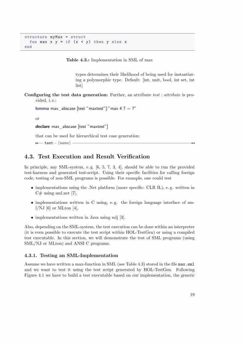
4.3.1. Testing an SML-Implementation
Assume we have written a max-function in SML (see Table 4.3) stored in the file max.smland we want to test it using the test script generated by HOL-TestGen. FollowingFigure 4.1 we have to build a test executable based on our implementation, the generic
19
Test Results:
=============
Test 0 - SUCCESS, result: 69
Test 1 - SUCCESS, result: ~11
Summary:
--------
Number successful tests cases: 2 of 2 (ca. 100%)
Number of warnings: 0 of 2 (ca. 0%)
Number of errors: 0 of 2 (ca. 0%)
Number of failures: 0 of 2 (ca. 0%)
Number of fatal errors: 0 of 2 (ca. 0%)
Overall result: success
===============
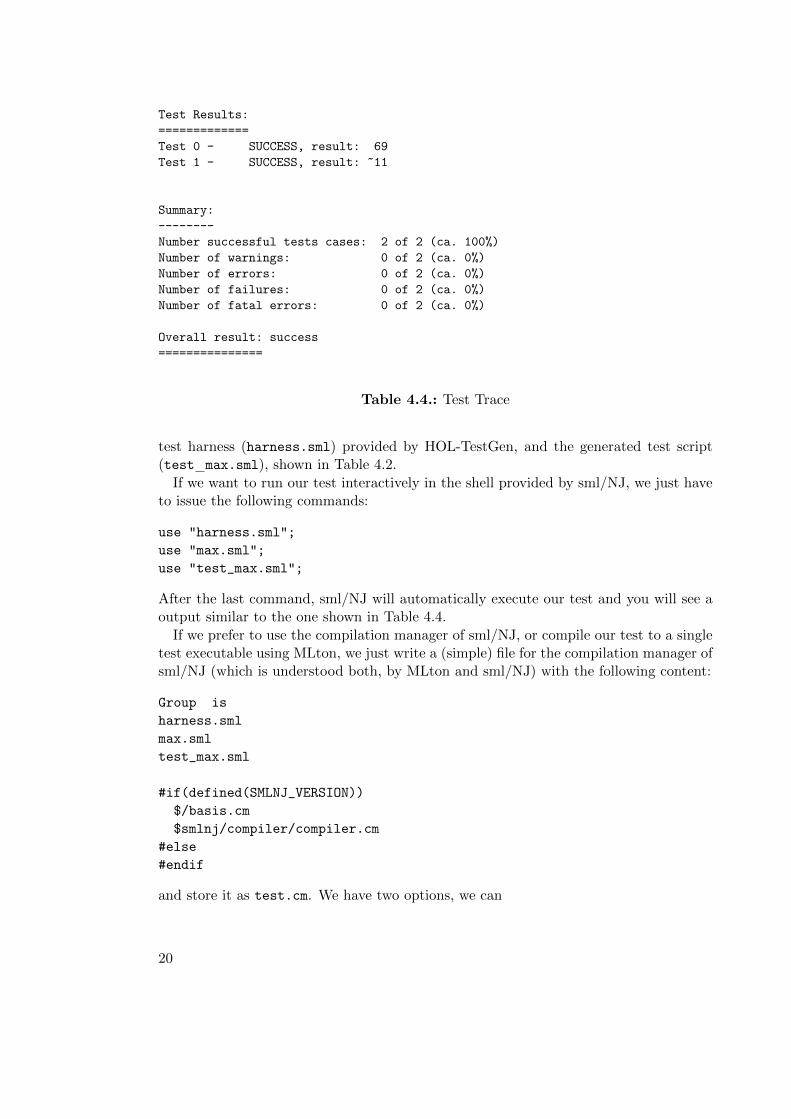
Table 4.4.: Test Trace
test harness (harness.sml) provided by HOL-TestGen, and the generated test script(test max.sml), shown in Table 4.2.
If we want to run our test interactively in the shell provided by sml/NJ, we just haveto issue the following commands:
use "harness.sml";
use "max.sml";
use "test_max.sml";
After the last command, sml/NJ will automatically execute our test and you will see aoutput similar to the one shown in Table 4.4.
If we prefer to use the compilation manager of sml/NJ, or compile our test to a singletest executable using MLton, we just write a (simple) file for the compilation manager ofsml/NJ (which is understood both, by MLton and sml/NJ) with the following content:
Group is
harness.sml
max.sml
test_max.sml
#if(defined(SMLNJ_VERSION))
$/basis.cm
$smlnj/compiler/compiler.cm
#else
#endif
and store it as test.cm. We have two options, we can
20
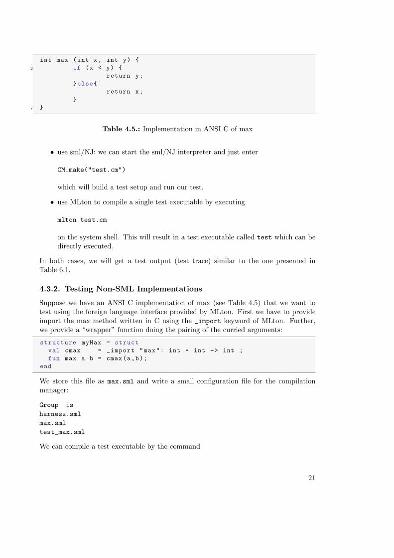
int max (int x, int y) {
2 if (x < y) {
return y;
}else{
return x;
}
7 }
Table 4.5.: Implementation in ANSI C of max
• use sml/NJ: we can start the sml/NJ interpreter and just enter
CM.make("test.cm")
which will build a test setup and run our test.
• use MLton to compile a single test executable by executing
mlton test.cm
on the system shell. This will result in a test executable called test which can bedirectly executed.
In both cases, we will get a test output (test trace) similar to the one presented inTable 6.1.
4.3.2. Testing Non-SML Implementations
Suppose we have an ANSI C implementation of max (see Table 4.5) that we want totest using the foreign language interface provided by MLton. First we have to provideimport the max method written in C using the _import keyword of MLton. Further,we provide a “wrapper” function doing the pairing of the curried arguments:
structure myMax = struct
val cmax = _import "max": int * int -> int ;
fun max a b = cmax(a,b);
end
We store this file as max.sml and write a small configuration file for the compilationmanager:
Group is
harness.sml
max.sml
test_max.sml
We can compile a test executable by the command
21
mlton -default-ann ’allowFFI true’ test.cm max.c
on the system shell. Again, we end up with an test executable test which can be calleddirectly. Running our test executable will result in trace similar to the one presented inTable 6.1.
4.4. Profiling Test Generation
HOL-TestGen includes support for profiling the test procedure. By default, profiling isturned off. Profiling can be turned on by issuing the command
-- profiling_on -�
Profiling can be turned off again with the command
-- profiling_off -�
When profiling is turned on, the time consumed by gen test cases and gen test datais recorded and associated with the test theorem. The profiling results can be printedby
-- print_clocks -�
A LaTeX version of the profiling results can be written to a file with the command
-- write_clocks 〈filename〉 -�
Users can also record the runtime of their own code. A time measurement can bestarted by issuing
-- start_clock 〈name〉 -�
where 〈name〉 is a name for identifying the time measured. The time measurement iscompleted by
-- stop_clock 〈name〉 -�
where 〈name〉 has to be the name used for the preceding start clock. If the names donot match, the profiling results are marked as erroneous. If several measurements areperformed using the same name, the times measured are added. The command
-- next_clock -�
proceeds to a new time measurement using a variant of the last name used.These profiling instructions can be nested, which causes the names used to be com-
bined to a path. The Clocks structure provides the tactic analogues start clock tac,stop clock tac and next clock tac to these commands. The profiling featuresavailable to the user are independent of HOL-TestGen’s profiling flag controlled by pro-filing on and profiling off.
22
5. Core Libraries
The core of HOL-TestGen comes with some infrastructure on key-concepts of testing.This includes
1. notions for test-sequences based on various state Monads,
2. notions for reactive test-sequences based on so-called observer theories (permittingthe handling of constraints occuring in reactive test sequences),
3. notions for automata allowing more complex forms of tests of refinements (inclusiontests, ioco, and friends).
Note that the latter parts of the theory library are still experimental.
5.1. Monads
theory Monads imports Main
begin
5.1.1. General Framework for Monad-based Sequence-Test
As such, Higher-order Logic as a purely functional specification formalism has no built-in mechanism for state and state-transitions. Forms of testing involving state requiretherefore explicit mechanisms for their treatment inside the logic; a well-known techniqueto model states inside purely functional languages are monads made popular by Wadlerand Moggi and extensively used in Haskell. HOL is powerful enough to represent themost important standard monads; however, it is not possible to represent monads assuch due to well-known limitations of the Hindley-Milner type-system.
Here is a variant for state-exception monads, that models precisely transition functionswith preconditions. Next, we declare the state-backtrack-monad. In all of them, ourconcept of i/o stepping functions can be formulated; these are functions mapping inputto a given monad. Later on, we will build the usual concepts of:
1. deterministic i/o automata,
2. non-deterministic i/o automata, and
3. labelled transition systems (LTS)
23
State Exception Monads
type synonym (’o, ’σ) MONSE = "’σ ⇀ (’o × ’σ)"
definition bind_SE :: "(’o,’σ)MONSE ⇒ (’o ⇒ (’o’,’σ)MONSE) ⇒ (’o’,’σ)MONSE"
where "bind_SE f g = (λσ. case f σ of None ⇒ None
| Some (out, σ’) ⇒ g out σ’)"
notation bind_SE ("bindSE")
syntax (xsymbols)
"_bind_SE" :: "[pttrn,(’o,’σ)MONSE,(’o’,’σ)MONSE] ⇒ (’o’,’σ)MONSE"
("(2 _ ← _; _)" [5,8,8]8)
translations"x ← f; g" == "CONST bind_SE f (% x . g)"
definition unit_SE :: "’o ⇒ (’o, ’σ)MONSE" ("(return _)" 8)
where "unit_SE e = (λσ. Some(e,σ))"notation unit_SE ("unitSE")
definition fail SE :: "(’o, ’σ)MONSE"
where "fail SE = (λσ. None)"
notation fail SE ("failSE")
definition assert_SE :: "(’σ ⇒ bool) ⇒ (bool, ’σ)MONSE"
where "assert_SE P = (λσ. if P σ then Some(True,σ) else None)"
notation assert_SE ("assertSE")
definition assume_SE :: "(’σ ⇒ bool) ⇒ (unit, ’σ)MONSE"
where "assume_SE P = (λσ. if ∃σ . P σ then Some((), SOME σ . P σ) else None)"
notation assume_SE ("assumeSE")
definition if_SE :: "[’σ ⇒ bool, (’α, ’σ)MONSE, (’α, ’σ)MONSE] ⇒ (’α, ’σ)MONSE"
where "if_SE c E F = (λσ. if c σ then E σ else F σ)"notation if_SE ("ifSE")
The bind-operator in the state-exception monad yields already a semantics for theconcept of an input sequence on the meta-level:
lemma syntax_test: "(o1 ← f1 ; o2 ← f2; return (post o1 o2)) = X"
oops
The standard monad theorems about unit and associativity:
lemma bind_left_unit : "(x ← return a; k) = k"
apply (simp add: unit_SE_def bind_SE_def)
done
lemma bind_right_unit: "(x ← m; return x) = m"
24
apply (simp add: unit_SE_def bind_SE_def)
apply (rule ext)
apply (case_tac "m σ", simp_all)
done
lemma bind_assoc: "(y ← (x ← m; k); h) = (x ← m; (y ← k; h))"
apply (simp add: unit_SE_def bind_SE_def, rule ext)
apply (case_tac "m σ", simp_all)
apply (case_tac "a", simp_all)
done
In order to express test-sequences also on the object-level and to make our theoryamenable to formal reasoning over test-sequences, we represent them as lists of input andgeneralize the bind-operator of the state-exception monad accordingly. The approach isstraightforward, but comes with a price: we have to encapsulate all input and output datainto one type. Assume that we have a typed interface to a module with the operationsop1, op2, . . . , opn with the inputs ι1, ι2, . . . , ιn (outputs are treated analogously). Thenwe can encode for this interface the general input - type:
datatype in = op1 :: ι1 | ... | ιn
Obviously, we loose some type-safety in this approach; we have to express that in tracesonly corresponding input and output belonging to the same operation will occur; thisform of side-conditions have to be expressed inside HOL. From the user perspective, thiswill not make much difference, since junk-data resulting from too weak typing can beruled out by adopted front-ends.
Note that the subsequent notion of a test-sequence allows the io stepping function(and the special case of a program under test) to stop execution within the sequence;such premature terminations are characterized by an output list which is shorter thanthe input list.
fun mbind :: "’ι list ⇒ (’ι ⇒ (’o,’σ) MONSE) ⇒ (’o list,’σ) MONSE"
where "mbind [] iostep σ = Some([], σ)" |
"mbind (a#H) iostep σ =
(case iostep a σ of
None ⇒ Some([], σ)| Some (out, σ’) ⇒ (case mbind H iostep σ’ of
None ⇒ Some([out],σ’)| Some(outs,σ’’) ⇒ Some(out#outs,σ’’)))"
This definition is fail-safe; in case of an exception, the current state is maintained. Analternative is the fail-strict variant mbind’ :
lemma mbind_unit [simp]:
"mbind [] f = (return [])"
by(rule ext, simp add: unit_SE_def)
lemma mbind_nofailure [simp]:
"mbind S f σ 6= None"
25
apply(rule_tac x=σ in spec)
apply(induct S, auto simp:unit_SE_def)
apply(case_tac "f a x", auto)
apply(erule_tac x="b" in allE)
apply(erule exE, erule exE, simp)
done
fun mbind’ :: "’ι list ⇒ (’ι ⇒ (’o,’σ) MONSE) ⇒ (’o list,’σ) MONSE"
where "mbind’ [] iostep σ = Some([], σ)" |
"mbind’ (a#H) iostep σ =
(case iostep a σ of
None ⇒ None
| Some (out, σ’) ⇒ (case mbind H iostep σ’ of
None ⇒ None (* fail-strict *)
| Some(outs,σ’’) ⇒ Some(out#outs,σ’’)))"
mbind’ as failure strict operator can be seen as a foldr on bind - if the types wouldmatch . . .
definition try_SE :: "(’o,’σ) MONSE ⇒ (’o option,’σ) MONSE"
where "try_SE ioprog = (λσ. case ioprog σ of
None ⇒ Some(None, σ)| Some(outs, σ’) ⇒ Some(Some outs, σ’))"
In contrast, mbind as a failure safe operator can roughly be seen as a foldr on bind- try: m1 ; try m2 ; try m3; ... Note, that the rough equivalence only holds for certainpredicates in the sequence - length equivalence modulo None, for example. However, ifa conditional is added, the equivalence can be made precise:
lemma mbind_try:
"(x ← mbind (a#S) F; M x) =
(a’ ← try_SE(F a);
if a’ = None
then (M [])
else (x ← mbind S F; M (the a’ # x)))"
apply(rule ext)
apply(simp add: bind_SE_def try_SE_def)
apply(case_tac "F a x", auto)
apply(simp add: bind_SE_def try_SE_def)
apply(case_tac "mbind S F b", auto)
done
On this basis, a symbolic evaluation scheme can be established that reduces mbind-code to try SE code and ite-cascades.
definition alt_SE :: "[(’o, ’σ)MONSE, (’o, ’σ)MONSE] ⇒ (’o, ’σ)MONSE"
( infixl "uSE" 10)
where "(f uSE g) = (λ σ. case f σ of None ⇒ g σ| Some H ⇒ Some H)"
definition malt_SE :: "(’o, ’σ)MONSE list ⇒ (’o, ’σ)MONSE"
26
where "malt_SE S = foldr alt_SE S failSE"
notation malt_SE ("d
SE")
lemma malt_SE_mt [simp]: "d
SE [] = failSE"
by(simp add: malt_SE_def)
lemma malt_SE_cons [simp]: "d
SE (a # S) = (a uSE (d
SE S))"
by(simp add: malt_SE_def)
State Backtrack Monads
This subsection is still rudimentary and as such an interesting formal analogue to theprevious monad definitions. It is doubtful that it is interesting for testing and as acmputational stucture at all. Clearly more relevant is “sequence” instead of “set,” whichwould rephrase Isabelle’s internal tactic concept.
type synonym (’o, ’σ) MONSB = "’σ ⇒ (’o × ’σ) set"
definition bind_SB :: "(’o, ’σ)MONSB ⇒ (’o ⇒ (’o’, ’σ)MONSB) ⇒ (’o’, ’σ)MONSB"
where "bind_SB f g σ =⋃
((λ(out, σ). (g out σ)) ‘ (f σ))"notation bind_SB ("bindSB")
definition unit_SB :: "’o ⇒ (’o, ’σ)MONSB" ("(returns _)" 8)
where "unit_SB e = (λσ. {(e,σ)})"notation unit_SB ("unitSB")
syntax (xsymbols)
"_bind_SB" :: "[pttrn,(’o,’σ)MONSB,(’o’,’σ)MONSB] ⇒ (’o’,’σ)MONSB"
("(2 _ := _; _)" [5,8,8]8)
translations"x := f; g" == "CONST bind_SB f (% x . g)"
lemma bind_left_unit_SB : "(x := returns a; m) = m"
by (rule ext,simp add: unit_SB_def bind_SB_def)
lemma bind_right_unit_SB: "(x := m; returns x) = m"
by (rule ext, simp add: unit_SB_def bind_SB_def)
lemma bind_assoc_SB: "(y := (x := m; k); h) = (x := m; (y := k; h))"
by (rule ext, simp add: unit_SB_def bind_SB_def split_def)
State Backtrack Exception Monad (vulgo: Boogie-PL)
The following combination of the previous two Monad-Constructions allows for the se-mantic foundation of a simple generic assertion language in the style of Schirmers Simpl-Language or Rustan Leino’s Boogie-PL language. The key is to use the exceptional
27
element None for violations of the assert-statement.
type synonym (’o, ’σ) MONSBE = "’σ ⇒ ((’o × ’σ) set) option"
definition bind_SBE :: "(’o,’σ)MONSBE ⇒ (’o ⇒ (’o’,’σ)MONSBE) ⇒ (’o’,’σ)MONSBE"
where "bind_SBE f g = (λσ. case f σ of None ⇒ None
| Some S ⇒ (let S’ = (λ(out, σ’). g out
σ’) ‘ S
in if None ∈ S’ then None
else Some(⋃
(the ‘ S’))))"
syntax (xsymbols)
"_bind_SBE" :: "[pttrn,(’o,’σ)MONSBE,(’o’,’σ)MONSBE] ⇒ (’o’,’σ)MONSBE"
("(2 _ :≡ _; _)" [5,8,8]8)
translations"x :≡ f; g" == "CONST bind_SBE f (% x . g)"
definition unit_SBE :: "’o ⇒ (’o, ’σ)MONSBE" ("(returning _)" 8)
where "unit_SBE e = (λσ. Some({(e,σ)}))"
definition assert_SBE :: "(’σ ⇒ bool) ⇒ (unit, ’σ)MONSBE"
where "assert_SBE e = (λσ. if e σ then Some({((),σ)})else None)"
notation assert_SBE ("assertSBE")
definition assume_SBE :: "(’σ ⇒ bool) ⇒ (unit, ’σ)MONSBE"
where "assume_SBE e = (λσ. if e σ then Some({((),σ)})else Some {})"
notation assume_SBE ("assumeSBE")
definition havoc_SBE :: " (unit, ’σ)MONSBE"
where "havoc_SBE = (λσ. Some({x. True}))"
notation havoc_SBE ("havocSBE")
lemma bind_left_unit_SBE : "(x :≡ returning a; m) = m"
apply (rule ext,simp add: unit_SBE_def bind_SBE_def)
apply (case_tac "m x",auto)
done
lemma bind_right_unit_SBE: "(x :≡ m; returning x) = m"
apply (rule ext, simp add: unit_SBE_def bind_SBE_def)
apply (case_tac "m x", simp_all add:Let_def)
apply (rule HOL.ccontr, simp add: Set.image_iff)
done
28
lemmas aux = trans[OF HOL.neq_commute,OF Option.not_None_eq]
lemma bind_assoc_SBE: "(y :≡ (x :≡ m; k); h) = (x :≡ m; (y :≡ k; h))"
proof (rule ext, simp add: unit_SBE_def bind_SBE_def,
case_tac "m x", simp_all add: Let_def Set.image_iff, safe)
case goal1 then show ?case
by(rule_tac x="(a, b)" in bexI, simp_all)
nextcase goal2 then show ?case
apply(rule_tac x="(aa, b)" in bexI, simp_all add:split_def)
apply(erule_tac x="(aa,b)" in ballE)
apply(auto simp: aux image_def split_def intro!: rev_bexI)
donenext
case goal3 then show ?case
by(rule_tac x="(a, b)" in bexI, simp_all)
nextcase goal4 then show ?case
apply(erule_tac Q="None = ?X" in contrapos_pp)
apply(erule_tac x="(aa,b)" and P="λ x. None 6= split (λout. k) x" in ballE)
apply(auto simp: aux Option.not_None_eq image_def split_def intro!: rev_bexI)
donenext
case goal5 then show ?case
apply simp apply((erule_tac x="(ab,ba)" in ballE)+)
apply(simp_all add: aux Option.not_None_eq, (erule exE)+, simp add:split_def)
apply(erule rev_bexI, case_tac "None∈(λp. h(snd p))‘y",auto simp:split_def)
done
nextcase goal6 then show ?case
apply simp apply((erule_tac x="(a,b)" in ballE)+)
apply(simp_all add: aux Option.not_None_eq, (erule exE)+, simp add:split_def)
apply(erule rev_bexI, case_tac "None∈(λp. h(snd p))‘y",auto simp:split_def)
doneqed
5.1.2. Valid Test Sequences in the State Exception Monad
This is still an unstructured merge of executable monad concepts and specification ori-ented high-level properties initiating test procedures.
definition valid_SE :: "’σ ⇒ (bool,’σ) MONSE ⇒ bool" ( infix "|=" 15)
where "(σ |= m) = (m σ 6= None ∧ fst(the (m σ)))"
This notation consideres failures as valid – a definition inspired by I/O conformance.BUG: It is not possible to define this concept once and for all in a Hindley-Milner type-system. For the moment, we present it only for the state-exception monad, although forthe same definition, this notion is applicable to other monads as well.
29
lemma syntax_test :
"σ |= (os ← (mbind ιs ioprog); return(length ιs = length os))"
oops
lemma valid_true[simp]:
"(σ |= (s ← return x ; return (P s))) = P x"
by(simp add: valid_SE_def unit_SE_def bind_SE_def)
Recall mbind_unit for the base case.
lemma valid_failure:
"ioprog a σ = None =⇒(σ |= (s ← mbind (a#S) ioprog ; M s)) =
(σ |= (M []))"
by(simp add: valid_SE_def unit_SE_def bind_SE_def)
lemmas valid_failure’’=valid_failure
lemma valid_failure’:
"A σ = None =⇒ ¬(σ |= ((s ← A ; M s)))"
by(simp add: valid_SE_def unit_SE_def bind_SE_def)
lemma valid_successElem:
"M σ = Some(f σ,σ) =⇒ (σ |= M) = f σ"by(simp add: valid_SE_def unit_SE_def bind_SE_def )
lemma valid_success:
"ioprog a σ = Some(b,σ’) =⇒(σ |= (s ← mbind (a#S) ioprog ; M s)) =
(σ’ |= (s ← mbind S ioprog ; M (b#s)))"
apply(simp add: valid_SE_def unit_SE_def bind_SE_def )
apply(cases "mbind S ioprog σ’", simp_all)
apply auto
done
lemma valid_success’’:
"ioprog a σ = Some(b,σ’) =⇒(σ |= (s ← mbind (a#S) ioprog ; return (P s))) =
(σ’ |= (s ← mbind S ioprog ; return (P (b#s))))"
apply(simp add: valid_SE_def unit_SE_def bind_SE_def )
apply(cases "mbind S ioprog σ’", simp_all)
apply auto
done
lemma valid_success’:
"A σ = Some(b,σ’) =⇒ (σ |= ((s ← A ; M s))) = (σ’ |= (M b))"
by(simp add: valid_SE_def unit_SE_def bind_SE_def )
30
lemma valid_both:
"(σ |= (s ← mbind (a#S) ioprog ; return (P s))) =
(case ioprog a σ of
None ⇒ (σ |= (return (P [])))
| Some(b,σ’) ⇒ (σ’ |= (s ← mbind S ioprog ; return (P (b#s)))))"
apply(case_tac "ioprog a σ")apply(simp_all add: valid_failure valid_success’’ split: prod.splits)
done
lemma valid_propagate_1 [simp]: "(σ |= (return P)) = (P)"
by(auto simp: valid_SE_def unit_SE_def)
lemma valid_propagate_2:
"σ |= ((s ← A ; M s)) =⇒∃ v σ’. the(A σ) = (v,σ’) ∧ σ’ |= (M v)"
apply(auto simp: valid_SE_def unit_SE_def bind_SE_def)
apply(cases "A σ", simp_all)
apply(simp add: Product_Type.prod_case_unfold)
apply(drule_tac x="A σ" and f=the in arg_cong, simp)
apply(rule_tac x="fst aa" in exI)
apply(rule_tac x="snd aa" in exI, auto)
done
lemma valid_propagate_2’:
"σ |= ((s ← A ; M s)) =⇒∃ a. (A σ) = Some a ∧ (snd a) |= (M (fst a))"
apply(auto simp: valid_SE_def unit_SE_def bind_SE_def)
apply(cases "A σ", simp_all)
apply(simp_all add: Product_Type.prod_case_unfold
split: prod.splits)
apply(drule_tac x="A σ" and f=the in arg_cong, simp)
apply(rule_tac x="fst aa" in exI)
apply(rule_tac x="snd aa" in exI, auto)
done
lemma valid_propagate_2’’:
"σ |= ((s ← A ; M s)) =⇒∃ v σ’. A σ = Some(v,σ’) ∧ σ’ |= (M v)"
apply(auto simp: valid_SE_def unit_SE_def bind_SE_def)
apply(cases "A σ", simp_all)
apply(simp add: Product_Type.prod_case_unfold)
apply(drule_tac x="A σ" and f=the in arg_cong, simp)
apply(rule_tac x="fst aa" in exI)
apply(rule_tac x="snd aa" in exI, auto)
done
31
lemma valid_propoagate_3[simp]: "(σ0 |= (λσ. Some (f σ, σ))) = (f σ0)"
by(simp add: valid_SE_def )
lemma valid_propoagate_3’[simp]: "¬(σ0 |= (λσ. None))"
by(simp add: valid_SE_def )
lemma assert_disch1 :" P σ =⇒ (σ |= (x ← assertSE P; M x)) = (σ |= (M True))"
by(auto simp: bind_SE_def assert_SE_def valid_SE_def)
lemma assert_disch2 :" ¬ P σ =⇒ ¬ (σ |= (x ← assertSE P ; M s))"
by(auto simp: bind_SE_def assert_SE_def valid_SE_def)
lemma assert_disch3 :" ¬ P σ =⇒ ¬ (σ |= (assertSE P))"
by(auto simp: bind_SE_def assert_SE_def valid_SE_def)
lemma assert_D : "(σ |= (x ← assertSE P; M x)) =⇒ P σ ∧ (σ |= (M True))"
by(auto simp: bind_SE_def assert_SE_def valid_SE_def split: HOL.split_if_asm)
lemma assume_D : "(σ |= (x ← assumeSE P; M x)) =⇒ ∃ σ. (P σ ∧ σ |= (M ()))"
apply(auto simp: bind_SE_def assume_SE_def valid_SE_def split: HOL.split_if_asm)
apply(rule_tac x="Eps P" in exI, auto)
apply(rule_tac x="True" in exI, rule_tac x="b" in exI)
apply(subst Hilbert_Choice.someI,assumption,simp)
apply(subst Hilbert_Choice.someI,assumption,simp)
done
These two rule prove that the SE Monad in connection with the notion of valid se-quence is actually sufficient for a representation of a Boogie-like language. The SBEmonad with explicit sets of states — to be shown below — is strictly speaking notnecessary (and will therefore be discontinued in the development).
lemma if_SE_D1 : "P σ =⇒ (σ |= ifSE P B1 B2) = (σ |= B1)"
by(auto simp: if_SE_def valid_SE_def)
lemma if_SE_D2 : "¬ P σ =⇒ (σ |= ifSE P B1 B2) = (σ |= B2)"
by(auto simp: if_SE_def valid_SE_def)
lemma if_SE_split_asm : " (σ |= ifSE P B1 B2) = ((P σ ∧ (σ |= B1)) ∨ (¬ P σ ∧(σ |= B2)))"
by(cases "P σ",auto simp: if_SE_D1 if_SE_D2)
lemma if_SE_split : " (σ |= ifSE P B1 B2) = ((P σ −→ (σ |= B1)) ∧ (¬ P σ −→(σ |= B2)))"
by(cases "P σ", auto simp: if_SE_D1 if_SE_D2)
lemma [code]:
"(σ |= m) = (case (m σ) of None ⇒ False | (Some (x,y)) ⇒ x)"
32
apply(simp add: valid_SE_def)
apply(cases "m σ = None", simp_all)
apply(insert not_None_eq, auto)
done
5.1.3. Valid Test Sequences in the State Exception Backtrack Monad
This is still an unstructured merge of executable monad concepts and specification ori-ented high-level properties initiating test procedures.
definition valid_SBE :: "’σ ⇒ (’a,’σ) MONSBE ⇒ bool" ( infix "|=SBE" 15)
where "σ |=SBE m ≡ (m σ 6= None)"
This notation consideres all non-failures as valid.
lemma assume_assert: "(σ |=SBE ( _ :≡ assumeSBE P ; assertSBE Q)) = (P σ −→Q σ)"
by(simp add: valid_SBE_def assume_SBE_def assert_SBE_def bind_SBE_def)
lemma assert_intro: "Q σ =⇒ σ |=SBE (assertSBE Q)"
by(simp add: valid_SBE_def assume_SBE_def assert_SBE_def bind_SBE_def)
lemma assume_dest:
"[[ σ |=SBE (x :≡ assumeSBE Q; M x); Q σ’ ]] =⇒ σ |=SBE M ()"
apply(auto simp: valid_SBE_def assume_SBE_def assert_SBE_def bind_SBE_def)
apply(cases "Q σ",simp_all)oops
This still needs work. What would be needed is a kind of wp - calculus that comesout of that. So far: nope.
end
5.2. Observers
theory Observers imports Monads
begin
5.2.1. IO-stepping Function Transfomers
The following adaption combinator converts an input-output program under test oftype: ι ⇒ σ ⇀ o × σ with program state σ into a state transition program that canbe processed by mbind. The key idea to turn mbind into a test-driver for a reactivesystem is by providing an internal state σ′, managed by the test driver, and external,problem-specific functions “rebind” and “substitute” that operate on this internal state.For example, this internal state can be instantiated with an environment var ⇀ value.The output (or parts of it) can then be bound to vars in the environment. In contrast,substitute can then explicit substitute variables occuring in value representations into
33
pure values, e.g. is can substitue c (”X”) into c 3 provided the environment containedthe map with X 3.
The state of the test-driver consists of two parts: the state of the observer (or: adaptor)σ and the internal state σ′ of the the step-function of the system under test ioprog isallowed to use.
definition observer :: "[’σ ⇒ ’o ⇒ ’σ, ’σ ⇒ ’ι ⇒ ’ι, ’σ×’σ’ ⇒ ’ι ⇒ ’o ⇒ bool]
⇒ (’ι ⇒ ’σ’ ⇀ ’o ×’σ’)⇒ (’ι ⇒ (’σ×’σ’ ⇀ ’σ×’σ’))"
where "observer rebind substitute postcond ioprog =
(λ input. (λ (σ, σ’). let input’= substitute σ input in
case ioprog input’ σ’ of
None ⇒ None (* ioprog failure - eg. timeout
... *)
| Some (output, σ’’’) ⇒ let σ’’ = rebind σ output
in
(if postcond (σ’’,σ’’’)input’ output
then Some(σ’’, σ’’’)else None (* postcond failure
*) )))"
The subsequent observer version is more powerful: it admits also preconditions ofioprog, which make reference to the observer state σobs. The observer-state may containan environment binding values to explicit variables. In such a scenario, the precond solvemay consist of a solver that constructs a solution from
1. this environment,
2. the observable state of the ioprog,
3. the abstract input (which may be related to a precondition which contains refer-ences to explicit variables)
such that all the explicit variables contained in the preconditions and the explicit vari-ables in the abstract input are substituted against values that make the preconditionstrue. The values must be stored in the environment and are reported in the observer-state σobs.
definition observer1 :: "[’σ_obs ⇒ ’o_c ⇒ ’σ_obs,’σ_obs ⇒ ’σ ⇒ ’ι_a ⇒ (’ι_c × ’σ_obs),’σ_obs ⇒ ’σ ⇒ ’ι_c ⇒ ’o_c ⇒ bool]
⇒ (’ι_c ⇒ (’o_c, ’σ)MONSE)
⇒ (’ι_a ⇒ (’o_c, ’σ_obs ×’σ)MONSE) "
where "observer1 rebind precond_solve postcond ioprog =
(λ in_a. (λ (σ_obs, σ). let (in_c,σ_obs’) = precond_solve σ_obs σ in_a
in case ioprog in_c σ of
34
None ⇒ None (* ioprog failure - eg. timeout
... *)
| Some (out_c, σ’) ⇒(let σ_obs’’ = rebind
σ_obs’ out_c
in if postcond σ_obs’’σ’ in_c out_c
then Some(out_c,
(σ_obs’, σ’))else None (* postcond
failure *) )))"
definition observer2 :: "[’σ_obs ⇒ ’o_c ⇒ ’σ_obs, ’σ_obs ⇒ ’ι_a ⇒ ’ι_c, ’σ_obs⇒ ’σ ⇒ ’ι_c ⇒ ’o_c ⇒ bool]
⇒ (’ι_c ⇒ (’o_c, ’σ)MONSE)
⇒ (’ι_a ⇒ (’o_c, ’σ_obs ×’σ)MONSE) "
where "observer2 rebind substitute postcond ioprog =
(λ in_a. (λ (σ_obs, σ). let in_c = substitute σ_obs in_a
in case ioprog in_c σ of
None ⇒ None (* ioprog failure - eg. timeout
... *)
| Some (out_c, σ’) ⇒(let σ_obs’ = rebind
σ_obs out_c
in if postcond σ_obs’σ’ in_c out_c
then Some(out_c,
(σ_obs’, σ’))else None (* postcond
failure *) )))"
Note that this version of the observer is just a monad-transformer; it transforms thei/o stepping function ioprog into another stepping function, which is the combined sub-system consisting of the observer and, for example, a program under test put . Theobserver takes the abstract input ina, substitutes explicit variables in it by concretevalues stored by its own state σobs and constructs concrete input inc, runs ioprog in thiscontext, and evaluates the return: the concrete output outc and the successor state σ′
are used to extract from concrete output concrete values and stores them inside its ownsuccessor state σ′obs. Provided that a post-condition is passed succesfully, the outputand the combined successor-state is reported as success.
Note that we made the following testability assumptions:
1. ioprog behaves wrt. to the reported state and input as a function, i.e. it behavesdeterministically, and
2. it is not necessary to destinguish internal failure and post-condition-failure. (Mod-elling Bug? This is superfluous and blind featurism ... One could do this by intro-ducing an own ”weakening”-monad endo-transformer.)
35
observer2 can actually be decomposed into two combinators - one dealing with themanagement of explicit variables and one that tackles post-conditions.
definition observer3 :: "[’σ_obs ⇒ ’o ⇒ ’σ_obs, ’σ_obs ⇒ ’ι_a ⇒ ’ι_c]⇒ (’ι_c ⇒ (’o, ’σ)MONSE)
⇒ (’ι_a ⇒ (’o, ’σ_obs ×’σ)MONSE) "
where "observer3 rebind substitute ioprog =
(λ in_a. (λ (σ_obs, σ).let in_c = substitute σ_obs in_a
in case ioprog in_c σ of
None ⇒ None (* ioprog failure - eg. timeout ... *)
| Some (out_c, σ’) ⇒(let σ_obs’ = rebind σ_obs out_c
in Some(out_c, (σ_obs’, σ’)) )))"
definition observer4 :: "[’σ ⇒ ’ι ⇒ ’o ⇒ bool]
⇒ (’ι ⇒ (’o, ’σ)MONSE)
⇒ (’ι ⇒ (’o, ’σ)MONSE)"
where "observer4 postcond ioprog =
(λ input. (λ σ. case ioprog input σ of
None ⇒ None (* ioprog failure - eg. timeout ... *)
| Some (output, σ’) ⇒ (if postcond σ’ input output
then Some(output, σ’)else None (* postcond failure *)
)))"
The following lemma explains the relationsship between observer2 and the decoposedversions observer3 and observer4. The full equality does not hold - the reason is thatthe two kinds of preconditions are different in a subtle way: the postcondition may makereference to the abstract state. (See our example Sequence_test based on a symbolicenvironment in the observer state.) If the postcondition does not do this, they areequivalent.
lemma observer_decompose:
" observer2 r s (λ x. pc) io = (observer3 r s (observer4 pc io))"
apply(rule ext, rule ext)
apply(auto simp: observer2_def observer3_def
observer4_def Let_def prod_case_beta)
apply(case_tac "io (s a x) b", auto)
done
end
36
5.3. Automata
theory Automata imports TestGen
begin
Re-Definition of the following type synonyms from Monad-Theory - apart from that,these theories are independent.
types (’o, ’σ) MON_SE = "’σ ⇀ (’o × ’σ)"types (’o, ’σ) MON_SB = "’σ ⇒ (’o × ’σ) set"
types (’o, ’σ) MON_SBE = "’σ ⇒ ((’o × ’σ) set) option"
Deterministic I/O automata (vulgo: programs)
record (’ι, ’o, ’σ) det_io_atm =
init :: "’σ"step :: "’ι ⇒ (’o, ’σ) MON_SE"
Nondeterministic I/O automata (vulgo: specifications)
We will use two styles of non-deterministic automata: Labelled Transition Systems(LTS), which are intensively used in the literature, but tend to anihilate the differencebetween input and output, and non-deterministic automata, which make this differenceexplicit and which have a closer connection to Monads used for the operational aspectsof testing.
There we are: labelled transition systems.
record (’ι, ’o, ’σ) lts =
init :: "’σ set"
step :: "(’σ × (’ι × ’o) × ’σ) set"
And, equivalently; non-deterministic io automata.
record (’ι, ’o, ’σ) ndet_io_atm =
init :: "’σ set"
step :: "’ι ⇒ (’o, ’σ) MON_SB"
First, we will prove the fundamental equivalence of these two notions.We refrain from a formal definition of explicit conversion functions and leave this
internally in this proof (i.e. the existential witnesses).
definition det2ndet :: "(’ι, ’o, ’σ) det_io_atm ⇒ (’ι, ’o, ’σ) ndet_io_atm"
where "det2ndet A = (|ndet_io_atm.init = {det_io_atm.init A},
ndet_io_atm.step =
λ ι σ. if σ ∈ dom(det_io_atm.step A ι)then {the(det_io_atm.step A ι σ)}else {} |)"
The following theorem estbalishes the fact that deterministic automata can be injec-tively embedded in non-deterministic ones.
lemma det2ndet_injective : "inj det2ndet"
37
apply(auto simp: inj_on_def det2ndet_def)
apply(tactic {* Record.split_simp_tac [] (K ~1) 1*}, simp)
apply(simp (no_asm_simp) add: fun_eq_iff, auto)
apply(drule_tac x=x in fun_cong, drule_tac x=xa in fun_cong)
apply(case_tac "xa ∈ dom (step x)", simp_all)
apply(case_tac "xa ∈ dom (stepa x)",
simp_all add: fun_eq_iff[symmetric], auto)
apply(case_tac "xa ∈ dom (stepa x)", auto simp: fun_eq_iff[symmetric])
apply(erule contrapos_np, simp)
apply(drule Product_Type.split_paired_All[THEN iffD2])+
apply(simp only: Option.not_Some_eq)
done
We distinguish two forms of determinism - global determinism, where for each stateand input at most one output-successor state is assigned.
definition deterministic :: "(’ι, ’o, ’σ) ndet_io_atm ⇒ bool"
where "deterministic atm = (((∃ x. ndet_io_atm.init atm = {x}) ∧(∀ ι out. ∀ p1 ∈ step atm ι out.
∀ p2 ∈ step atm ι out.
p1 = p2)))"
In contrast, transition relations
definition σdeterministic :: "(’ι, ’o, ’σ) ndet_io_atm ⇒ bool"
where "σdeterministic atm = (∃ x. ndet_io_atm.init atm = {x} ∧(∀ ι out.
∀ p1 ∈ step atm ι out.
∀ p2 ∈ step atm ι out.
fst p1 = fst p2 −→ snd p1 = snd p2))"
lemma det2ndet_deterministic:
"deterministic (det2ndet atm)"
by(auto simp:deterministic_def det2ndet_def)
lemma det2ndet_σdeterministic:"σdeterministic (det2ndet atm)"
by(auto simp: σdeterministic_def det2ndet_def)
The following theorem establishes the isomorphism of the two concepts IO-Automataand LTS. We will therefore concentrate in the sequel on IO-Automata, which have aslightly more realistic operational behaviour: you give the program under test an inputand get a possible set of responses rather than ”agreeing with the program under test”on a set of input-output-pairs.
definition ndet2lts :: "(’ι, ’o, ’σ) ndet_io_atm ⇒ (’ι, ’o, ’σ) lts"
where "ndet2lts A = (|lts.init = init A,
lts.step = {(s,io,s’).(snd io,s’) ∈ step A (fst io) s}|)"
definition lts2ndet :: " (’ι,’o,’σ) lts ⇒ (’ι, ’o, ’σ) ndet_io_atm"
where "lts2ndet A = (|init = lts.init A,
38
step = λ i s. {(out,s’). (s, (i,out), s’)
∈ lts.step A}|)"
lemma ndet_io_atm_isomorph_lts : "bij ndet2lts"
apply (auto simp: bij_def inj_on_def surj_def ndet2lts_def)
apply (tactic {* Record.split_simp_tac [] (K ~1) 1*}, simp)
apply (rule ext, rule ext, simp add: set_eq_iff)
apply (rule_tac x = "lts2ndet y" in exI)
apply (simp add: lts2ndet_def)
done
The following well-formedness property is important: for every state, there is a validtransition. Otherwise, some states may never be part of an (infinite) trace.
definition is_enabled :: "[’ι ⇒ (’o, ’σ) MON_SB, ’σ ] ⇒ bool"
where "is_enabled rel σ = (∃ ι. rel ι σ 6= {})"
definition is_enabled’ :: "[’ι ⇒ (’o, ’σ) MON_SE, ’σ ] ⇒ bool"
where "is_enabled’ rel σ = (∃ ι. σ ∈ dom(rel ι))"
definition live_wff:: "(’ι, ’o, ’σ) ndet_io_atm ⇒ bool"
where "live_wff atm = (∀ σ. ∃ ι. step atm ι σ 6= {})"
lemma life_wff_charn:
"live_wff atm = (∀ σ. is_enabled (step atm) σ)"by(auto simp: live_wff_def is_enabled_def)
There are essentialy two approaches: either we disallow non-enabled transition systems— via life wff charn — or we restrict our machinery for traces and prefixed closed setsof runs over them
5.3.1. Rich Traces and its Derivatives
The easiest way to define the concept of traces is on LTS. Via the injections describedabove, we can define notions like deterministic automata rich trace, and i/o automatarich trace. Moreover, we can easily project event traces or state traces from rich traces.
types (’ι, ’o, ’σ) trace = "nat ⇒ (’σ × (’ι × ’o) × ’σ)"(’ι, ’o) etrace = "nat ⇒ (’ι × ’o)"
’σ σtrace = "nat ⇒ ’σ"’ι in_trace = "nat ⇒ ’ι"’o out_trace = "nat ⇒ ’o"
(’ι, ’o, ’σ) run = "(’σ × (’ι × ’o) × ’σ) list"
(’ι, ’o) erun = "(’ι × ’o) list"
’σ σrun = "’σ list"
’ι in_run = "’ι list"
’o out_run = "’o list"
definition rtraces ::"(’ι, ’o, ’σ) ndet_io_atm ⇒ (’ι, ’o, ’σ) trace set"
39
where "rtraces atm = { t. fst(t 0) ∈ init atm ∧(∀ n. fst(t (Suc n)) = snd(snd(t n))) ∧(∀ n. if is_enabled (step atm) (fst(t n))
then t n ∈ {(s,io,s’). (snd io,s’)
∈ step atm (fst io) s}
else t n = (fst(t n),undefined,fst(t n)))}"
lemma init_rtraces[elim!]: "t ∈ rtraces atm =⇒ fst(t 0) ∈ init atm"
by(auto simp: rtraces_def)
lemma post_is_pre_state[elim!]: "t ∈ rtraces atm =⇒ fst(t (Suc n)) = snd(snd(t
n))"
by(auto simp: rtraces_def)
lemma enabled_transition[elim!]:
"[[t ∈ rtraces atm; is_enabled (step atm) (fst(t n)) ]]=⇒ t n ∈ {(s,io,s’). (snd io,s’) ∈ step atm (fst io) s}"
apply(simp add: rtraces_def split_def, safe)
apply(erule_tac x=n andP="λ n. if (?X n) then (?Y n) else (?Z n)"
in allE)
apply(simp add: split_def)
done
lemma nonenabled_transition[elim!]:
"[[t ∈ rtraces atm; ¬ is_enabled (step atm) (fst(t n)) ]]=⇒ t n = (fst(t n),undefined,fst(t n))"
by(simp add: rtraces_def split_def)
The latter definition solves the problem of inherently finite traces, i.e. those that reacha state in which they are no longer enabled. They are represented by stuttering stepson the same state.
definition fin_rtraces :: "(’ι, ’o, ’σ) ndet_io_atm ⇒ (’ι, ’o, ’σ) trace set"
where "fin_rtraces atm = { t . t ∈ rtraces atm ∧(∃ n. ¬ is_enabled (step atm) (fst(t n)))}"
lemma fin_rtraces_are_rtraces : "fin_rtraces atm ⊆ rtraces atm"
by(auto simp: rtraces_def fin_rtraces_def)
definition σtraces ::"(’ι, ’o, ’σ) ndet_io_atm ⇒ ’σ σtrace set"
where "σtraces atm = {t . ∃ rt ∈ rtraces atm. t = fst o rt }"
definition etraces ::"(’ι, ’o, ’σ) ndet_io_atm ⇒ (’ι, ’o) etrace set"
where "etraces atm = {t . ∃ rt ∈ rtraces atm. t = fst o snd o rt }"
definition in_trace :: "(’ι, ’o) etrace ⇒ ’ι in_trace"
where "in_trace rt = fst o rt"
40
definition out_trace :: "(’ι, ’o) etrace ⇒ ’o out_trace"
where "out_trace rt = snd o rt"
definition prefixes :: "(nat ⇒ ’α) set ⇒ ’α list set"
where "prefixes ts = {l. ∃ t ∈ ts. ∃ (n::int). l = map (t o nat) [0..n]}"
definition rprefixes :: "[’ι ⇒ (’o, ’σ) MON_SB,
(’ι, ’o, ’σ) trace set] ⇒ (’ι, ’o, ’σ) run set"
where "rprefixes rel ts = {l. ∃ t ∈ ts. ∃ n. (is_enabled rel (fst(t (nat n)))
∧l = map (t o nat) [0..n])}"
definition eprefixes :: "[’ι ⇒ (’o, ’σ) MON_SB,
(’ι, ’o, ’σ) trace set] ⇒ (’ι, ’o) erun set"
where "eprefixes rel ts = (map (fst o snd)) ‘ (rprefixes rel ts)"
definition σprefixes :: "[’ι ⇒ (’o, ’σ) MON_SB,
(’ι, ’o, ’σ) trace set] ⇒ ’σ σrun set"
where "σprefixes rel ts = (map fst) ‘ (rprefixes rel ts)"
5.3.2. Extensions: Automata with Explicit Final States
We model a few widely used variants of automata as record extensions. In particular,we define automata with final states and internal (output) actions.
record (’ι, ’o, ’σ) det_io_atm’ = "(’ι, ’o, ’σ) det_io_atm" +
final :: "’σ set"
A natural well-formedness property to be required from this type of atm is as follows:whenever an atm’ is in a final state, the transition operation is undefined.
definition final_wff:: "(’ι, ’o, ’σ) det_io_atm’ ⇒ bool"
where "final_wff atm’ =
(∀σ ∈ final atm’. ∀ ι. σ /∈ dom (det_io_atm.step atm’ ι))"
Another extension provides the concept of internal actions – which are considered aspart of the output alphabet here. If internal actions are also used for synchronization,further extensions admitting internal input actions will be necessary, too, which we donot model here.
record (’ι, ’o, ’σ) det_io_atm’’ = "(’ι, ’o, ’σ) det_io_atm’" +
internal :: "’o set"
A natural well-formedness property to be required from this type of atm is as follows:whenever an atm’ is in a final state, the transition operation is required to provide astate that is again final and an output that is considered internal.
definition final_wff2:: "(’ι, ’o, ’σ) det_io_atm’’ ⇒ bool"
where "final_wff2 atm’’ = (∀σ ∈ final atm’’.
∀ ι. σ ∈ dom (det_io_atm.step atm’’ ι) −→(let (out, σ’) = the(det_io_atm.step atm’’ ι σ)in out ∈ internal atm’’ ∧ σ’ ∈ final atm’’))"
41
Of course, for this type of extended automata, it is also possible to impose the ad-ditional requirement that the step function is total – undefined steps would then berepresented as steps leading to final states.
The standard extensions on deterministic automata are also redefined for the non-deterministic (specification) case.
record (’ι, ’o, ’σ) ndet_io_atm’ = "(’ι, ’o, ’σ) ndet_io_atm" +
final :: "’σ set"
definition final_wff_ndet_io_atm2 :: "(’ι, ’o, ’σ) ndet_io_atm’ ⇒ bool"
where "final_wff_ndet_io_atm2 atm’ = (∀σ ∈ final atm’. ∀ ι. ndet_io_atm.step atm’
ι σ = {})"
record (’ι, ’o, ’σ) ndet_io_atm’’ = "(’ι, ’o, ’σ) ndet_io_atm’" +
internal :: "’o set"
definition final_wff2_ndet_io_atm2 :: "(’ι, ’o, ’σ) ndet_io_atm’’ ⇒ bool"
where "final_wff2_ndet_io_atm2 atm’’ =
(∀σ ∈ final atm’’.
∀ ι. step atm’’ ι σ 6= {} −→ step atm’’ ι σ ⊆ internal
atm’’ × final atm’’)"
end
5.4. TestRefinements
theory TestRefinements imports Monads Automata
begin
5.4.1. Conversions Between Programs and Specifications
Some generalities: implementations and implementability
A (standard) implementation to a specification is just:
definition impl :: "[’σ⇒’ι⇒bool, ’ι ⇒ (’o,’σ)MON_SB] ⇒ ’ι ⇒ (’o,’σ)MON_SE"where "impl pre post ι = (λ σ. if pre σ ι
then Some(SOME(out,σ’). post ι σ (out,σ’))else undefined)"
definition strong_impl :: "[’σ⇒’ι⇒bool, ’ι⇒(’o,’σ)MON_SB] ⇒ ’ι⇒(’o, ’σ)MON_SE"where "strong_impl pre post ι =
(λ σ. if pre σ ιthen Some(SOME(out,σ’). post ι σ (out,σ’))else None)"
42
definition implementable :: "[’σ ⇒ ’ι ⇒ bool,’ι ⇒ (’o,’σ)MON_SB] ⇒ bool"
where "implementable pre post =(∀ σ ι. pre σ ι −→(∃ out σ’. post ι σ (out,σ’)))"
definition is_strong_impl :: "[’σ ⇒ ’ι ⇒ bool,
’ι ⇒ (’o,’σ)MON_SB,’ι ⇒ (’o, ’σ)MON_SE] ⇒ bool"
where "is_strong_impl pre post ioprog =
(∀ σ ι. (¬pre σ ι ∧ ioprog ι σ = None) ∨(pre σ ι ∧ (∃ x. ioprog ι σ = Some x)))"
lemma is_strong_impl :
"is_strong_impl pre post (strong_impl pre post)"
by(simp add: is_strong_impl_def strong_impl_def)
This following characterization of implementable specifications has actually a quitecomplicated form due to the fact that post expects its arguments in curried form -should be improved . . .
lemma implementable_charn:
"[[implementable pre post; pre σ ι ]] =⇒post ι σ (the(strong_impl pre post ι σ))"
apply(auto simp: implementable_def strong_impl_def)
apply(erule_tac x=σ in allE)
apply(erule_tac x=ι in allE)
apply(simp add: Eps_split)
apply(rule someI_ex, auto)
done
converts infinite trace sets to prefix-closed sets of finite traces, reconciling the mostcommon different concepts of traces ...
consts cnv :: "(nat ⇒ ’α) ⇒ ’α list"
consts input_refine ::
"[(’ι,’o,’σ) det_io_atm,(’ι,’o,’σ) ndet_io_atm] ⇒ bool"
consts input_output_refine ::
"[(’ι,’o,’σ) det_io_atm,(’ι,’o,’σ) ndet_io_atm] ⇒ bool"
notation input_refine ("(_/ vI _)" [51, 51] 50)
defs input_refine_def:
"I vI SP ≡({det_io_atm.init I} = ndet_io_atm.init SP) ∧(∀ t ∈ cnv ‘ (in_trace ‘(etraces SP)).
(det_io_atm.init I)
|= (os ← (mbind t (det_io_atm.step I)) ;
return(length t = length os)))"
This testing notion essentially says: whenever we can run an input sequence succesfullyon the PUT (the program does not throw an exception), it is ok.
43

notation input_output_refine ("(_/ vIO _)" [51, 51] 50)
defs input_output_refine_def:
"input_output_refine i s ≡({det_io_atm.init i} = ndet_io_atm.init s) ∧(∀ t ∈ prefixes (etraces s).
(det_io_atm.init i)
|= (os ← (mbind (map fst t) (det_io_atm.step i));
return((map snd t) = os)))"
Our no-frills-approach to I/O conformance testing: no quiescense, and strict alterna-tion between input and output.
PROBLEM : Tretmanns / Belinfantes notion of ioco is inherently different fromGaudels, which is refusal based. See definition in accompanying IOCO.thy file:
definition ioco :: "[(’\<iota>,’o option,’\<sigma>)IO_TS,(’\<iota>,’o option,’\<sigma>)IO_TS] \<Rightarrow> bool"
(infixl "ioco" 200)
"i ioco s \<equiv> (\<forall> t \<in> Straces(s).
out i (i after t) \<subseteq> out s (s after t))"
definition after :: "[(’ι, ’o, ’σ) ndet_io_atm, (’ι × ’o) list] ⇒ ’σ set"
( infixl "after" 100)
where "atm after l = {σ’ . ∃ t ∈ rtraces atm. (σ’ = fst(t (length l)) ∧(∀ n ∈ {0 .. (length l) - 1}. l!n = fst(snd(t n))))}"
definition out :: "[(’ι, ’o, ’σ) ndet_io_atm,’σ set, ’ι] ⇒ ’o set"
where "out atm ss ι = {a. ∃σ ∈ ss. ∃σ’. (a,σ’) ∈ ndet_io_atm.step atm ι σ}"
definition ready :: "[(’ι, ’o, ’σ) ndet_io_atm,’σ set] ⇒ ’ι set"
where "ready atm ss = {ι. ∃σ ∈ ss. ndet_io_atm.step atm ι σ 6= {}}"
definition ioco :: "[(’ι,’o,’σ)ndet_io_atm, (’ι,’o,’σ)ndet_io_atm] ⇒ bool"
( infixl "ioco" 200)
where "i ioco s = (∀ t ∈ prefixes(etraces s).
∀ ι ∈ ready s (s after t).
out i (i after t) ι ⊆ out s (s after t) ι)"
definition oico :: "[(’ι,’o,’σ)ndet_io_atm,(’ι,’o,’σ)ndet_io_atm] ⇒ bool"
( infixl "oico" 200)
where "i oico s = (∀ t ∈ prefixes(etraces s).
ready i (i after t) ⊇ ready s (s after t))"
definition ioco2 :: "[(’ι,’o,’σ)ndet_io_atm, (’ι,’o,’σ)ndet_io_atm] ⇒ bool"
( infixl "ioco2" 200)
where "i ioco2 s = (∀ t ∈ eprefixes (ndet_io_atm.step s) (rtraces s).
44
∀ ι ∈ ready s (s after t).
out i (i after t) ι ⊆ out s (s after t) ι)"
definition ico :: "[(’ι, ’o, ’σ) det_io_atm,(’ι, ’o, ’σ) ndet_io_atm] ⇒ bool"
( infixl "ico" 200)
where "i ico s = (∀ t ∈ prefixes(etraces s).
let i’ = det2ndet i
in ready i’ (i’ after t) ⊇ ready s (s after t))"
lemma full_det_refine: "s = det2ndet s’ =⇒(det2ndet i) ioco s ∧ (det2ndet i) oico s ←→ input_output_refine i s"
apply(safe)oops
definition ico2 :: "[(’ι,’o,’σ)ndet_io_atm,(’ι,’o,’σ)ndet_io_atm] ⇒ bool"
( infixl "ico2" 200)
where "i ico2 s ≡ ∀ t ∈ eprefixes (ndet_io_atm.step s) (rtraces s).
ready i (i after t) ⊇ ready s (s after t)"
There is lots of potential for optimization.
• only maximal prefixes
• draw the ω tests inside the return
• compute the ω by the ioprog , not quantify over it.
end
45

6. Examples
Before introducing the HOL-TestGen showcase ranging from simple to more advancedexamples, one general remark: The test data generation uses as final procedure to solvethe constraints of test cases a random solver. This choice has the advantage that therandom process is faster in general while requiring less interaction as, say, an enumerationbased solution principle. However this choice has the feature that two different runs ofthis document will produce outputs that differ in the details of displayed data. Evenworse, in very unlikely cases, the random solver does not find a solution that a previousrun could easily produce. In such cases, one should upgrade the iterations-variable inthe test environment.
6.1. Max
theorymax_test
importsTesting
begin
This introductory example explains the standard HOL-TestGen method resulting ina formalized test plan that is documented in a machine-checked text like this theorydocument.
We declare the context of this document—which must be the theory “Testing” at leastin order to include the HOL-TestGen system libraries—and the type of the programunder test.
consts prog :: "int ⇒ int ⇒ int"
Assume we want to test a simple program computing the maximum value of twointegers. We start by writing our test specification:
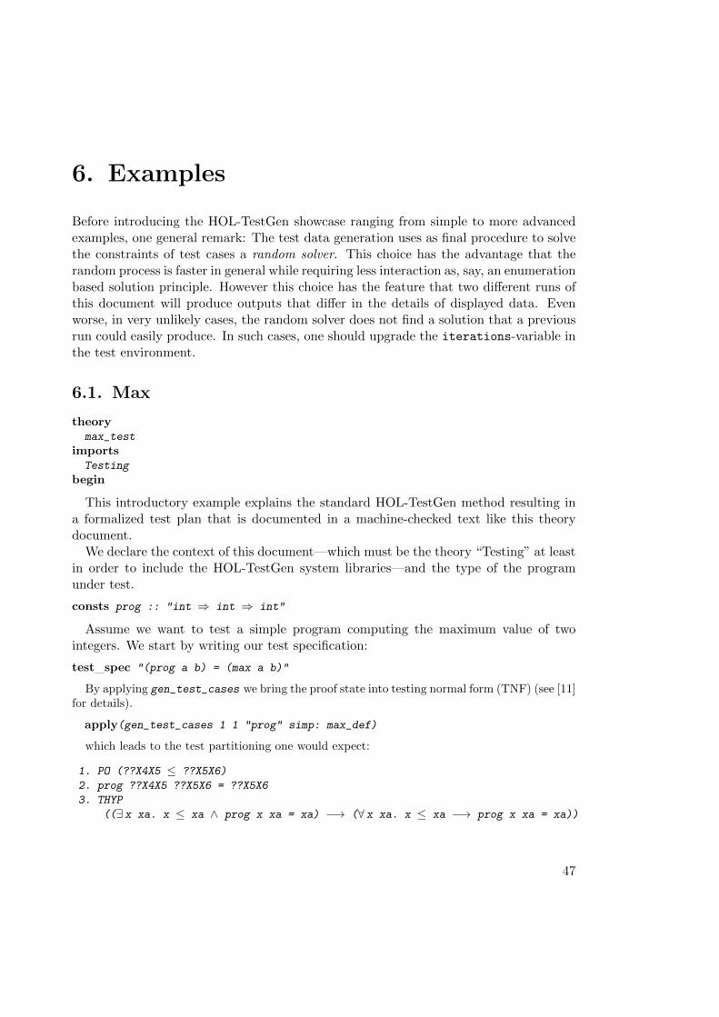
test spec "(prog a b) = (max a b)"
By applying gen_test_cases we bring the proof state into testing normal form (TNF) (see [11]for details).
apply(gen_test_cases 1 1 "prog" simp: max_def)
which leads to the test partitioning one would expect:
1. PO (??X4X5 ≤ ??X5X6)
2. prog ??X4X5 ??X5X6 = ??X5X6
3. THYP
((∃ x xa. x ≤ xa ∧ prog x xa = xa) −→ (∀ x xa. x ≤ xa −→ prog x xa = xa))
47
4. PO (¬ ??X1X5 ≤ ??X2X6)
5. prog ??X1X5 ??X2X6 = ??X1X5
6. THYP
((∃ x xa. ¬ x ≤ xa ∧ prog x xa = x) −→(∀ x xa. ¬ x ≤ xa −→ prog x xa = x))
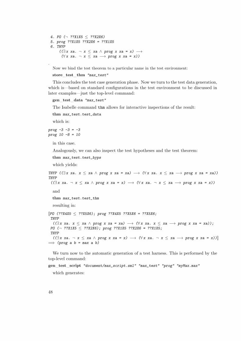
.Now we bind the test theorem to a particular name in the test environment:
store test thm "max_test"
This concludes the test case generation phase. Now we turn to the test data generation,which is—based on standard configurations in the test environment to be discussed inlater examples—just the top-level command:
gen test data "max_test"
The Isabelle command thm allows for interactive inspections of the result:
thm max_test.test_data
which is:
prog -3 -3 = -3
prog 10 -8 = 10
in this case.
Analogously, we can also inspect the test hypotheses and the test theorem:
thm max_test.test_hyps
which yields:
THYP ((∃ x xa. x ≤ xa ∧ prog x xa = xa) −→ (∀ x xa. x ≤ xa −→ prog x xa = xa))
THYP
((∃ x xa. ¬ x ≤ xa ∧ prog x xa = x) −→ (∀ x xa. ¬ x ≤ xa −→ prog x xa = x))
and
thm max_test.test_thm
resulting in:
[[PO (??X4X5 ≤ ??X5X6); prog ??X4X5 ??X5X6 = ??X5X6;
THYP
((∃ x xa. x ≤ xa ∧ prog x xa = xa) −→ (∀ x xa. x ≤ xa −→ prog x xa = xa));
PO (¬ ??X1X5 ≤ ??X2X6); prog ??X1X5 ??X2X6 = ??X1X5;
THYP
((∃ x xa. ¬ x ≤ xa ∧ prog x xa = x) −→ (∀ x xa. ¬ x ≤ xa −→ prog x xa = x))]]=⇒ (prog a b = max a b)
We turn now to the automatic generation of a test harness. This is performed by thetop-level command:
gen test script "document/max_script.sml" "max_test" "prog" "myMax.max"
which generates:
48
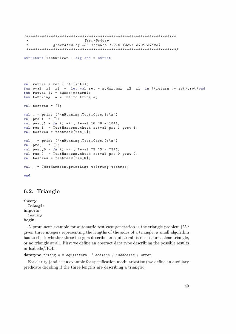
(* ******************************************************************
* Test -Driver
* generated by HOL -TestGen 1.7.0 (dev: 8725:8750M)
****************************************************************** *)
structure TestDriver : sig end = struct
val return = ref ( ~4:( int ));
fun eval x2 x1 = let val ret = myMax.max x2 x1 in (( return := ret);ret)end
fun retval () = SOME(! return );
fun toString a = Int.toString a;
val testres = [];
val _ = print ("\nRunning Test Case 1:\n")
val pre_1 = [];
val post_1 = fn () => ( (eval 10 ~8 = 10));
val res_1 = TestHarness.check retval pre_1 post_1;
val testres = testres@[res_1];
val _ = print ("\nRunning Test Case 0:\n")
val pre_0 = [];
val post_0 = fn () => ( (eval ~3 ~3 = ~3));
val res_0 = TestHarness.check retval pre_0 post_0;
val testres = testres@[res_0];
val _ = TestHarness.printList toString testres;
end
6.2. Triangle
theoryTriangle
importsTesting
begin
A prominent example for automatic test case generation is the triangle problem [25]:given three integers representing the lengths of the sides of a triangle, a small algorithmhas to check whether these integers describe an equilateral, isosceles, or scalene triangle,or no triangle at all. First we define an abstract data type describing the possible resultsin Isabelle/HOL:
datatype triangle = equilateral | scalene | isosceles | error
For clarity (and as an example for specification modularization) we define an auxiliarypredicate deciding if the three lengths are describing a triangle:
49
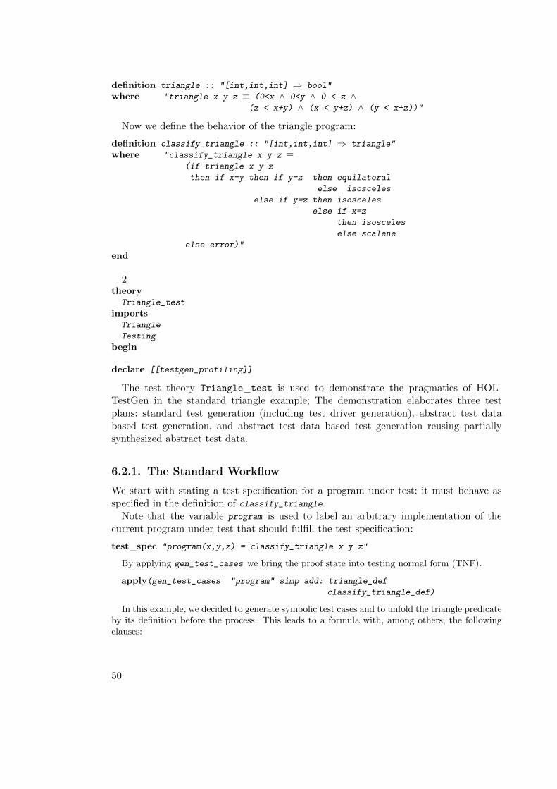
definition triangle :: "[int,int,int] ⇒ bool"
where "triangle x y z ≡ (0<x ∧ 0<y ∧ 0 < z ∧(z < x+y) ∧ (x < y+z) ∧ (y < x+z))"
Now we define the behavior of the triangle program:
definition classify_triangle :: "[int,int,int] ⇒ triangle"
where "classify_triangle x y z ≡(if triangle x y z
then if x=y then if y=z then equilateral
else isosceles
else if y=z then isosceles
else if x=z
then isosceles
else scalene
else error)"
end
2theoryTriangle_test
importsTriangle
Testing
begin
declare [[testgen_profiling]]
The test theory Triangle test is used to demonstrate the pragmatics of HOL-TestGen in the standard triangle example; The demonstration elaborates three testplans: standard test generation (including test driver generation), abstract test databased test generation, and abstract test data based test generation reusing partiallysynthesized abstract test data.
6.2.1. The Standard Workflow
We start with stating a test specification for a program under test: it must behave asspecified in the definition of classify_triangle.
Note that the variable program is used to label an arbitrary implementation of thecurrent program under test that should fulfill the test specification:
test spec "program(x,y,z) = classify_triangle x y z"
By applying gen_test_cases we bring the proof state into testing normal form (TNF).
apply(gen_test_cases "program" simp add: triangle_def
classify_triangle_def)
In this example, we decided to generate symbolic test cases and to unfold the triangle predicateby its definition before the process. This leads to a formula with, among others, the followingclauses:
50
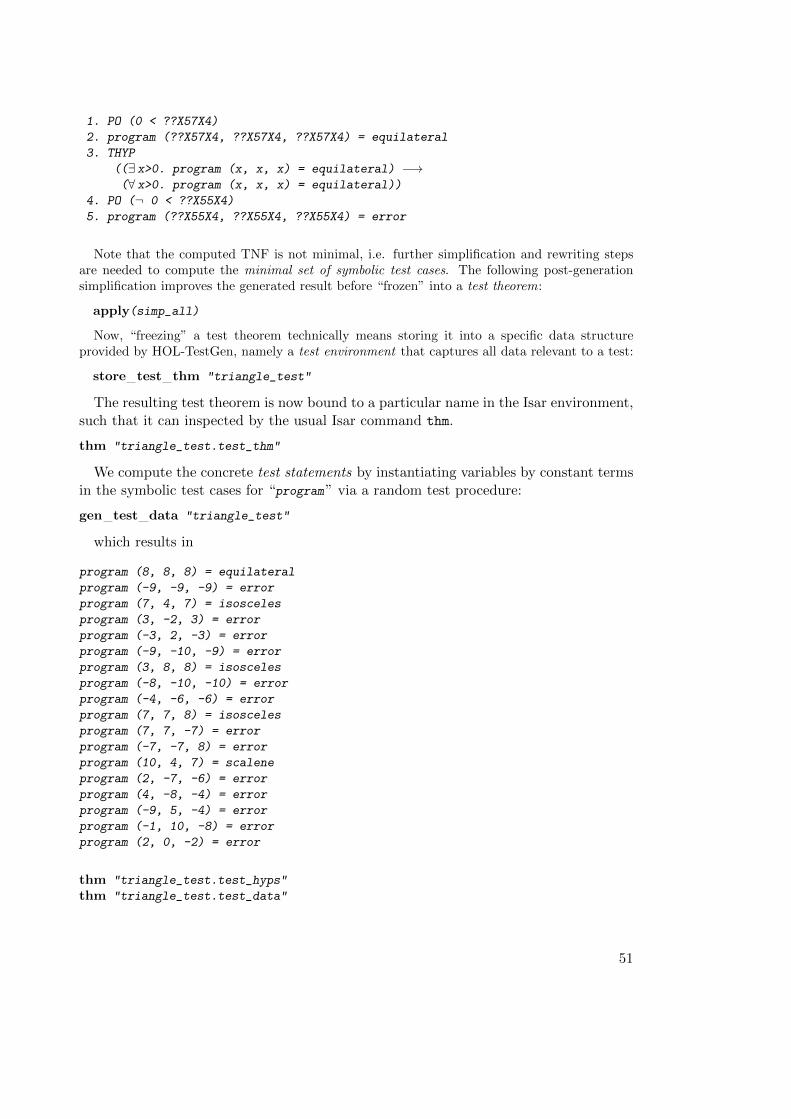
1. PO (0 < ??X57X4)
2. program (??X57X4, ??X57X4, ??X57X4) = equilateral
3. THYP
((∃ x>0. program (x, x, x) = equilateral) −→(∀ x>0. program (x, x, x) = equilateral))
4. PO (¬ 0 < ??X55X4)
5. program (??X55X4, ??X55X4, ??X55X4) = error
Note that the computed TNF is not minimal, i.e. further simplification and rewriting stepsare needed to compute the minimal set of symbolic test cases. The following post-generationsimplification improves the generated result before “frozen” into a test theorem:
apply(simp_all)
Now, “freezing” a test theorem technically means storing it into a specific data structureprovided by HOL-TestGen, namely a test environment that captures all data relevant to a test:
store test thm "triangle_test"
The resulting test theorem is now bound to a particular name in the Isar environment,such that it can inspected by the usual Isar command thm.
thm "triangle_test.test_thm"
We compute the concrete test statements by instantiating variables by constant termsin the symbolic test cases for “program” via a random test procedure:
gen test data "triangle_test"
which results in
program (8, 8, 8) = equilateral
program (-9, -9, -9) = error
program (7, 4, 7) = isosceles
program (3, -2, 3) = error
program (-3, 2, -3) = error
program (-9, -10, -9) = error
program (3, 8, 8) = isosceles
program (-8, -10, -10) = error
program (-4, -6, -6) = error
program (7, 7, 8) = isosceles
program (7, 7, -7) = error
program (-7, -7, 8) = error
program (10, 4, 7) = scalene
program (2, -7, -6) = error
program (4, -8, -4) = error
program (-9, 5, -4) = error
program (-1, 10, -8) = error
program (2, 0, -2) = error
thm "triangle_test.test_hyps"
thm "triangle_test.test_data"
51

Now we use the generated test data statement lists to automatically generate a testdriver, which is controlled by the test harness. The first argument is the external SML-file name into which the test driver is generated, the second argument the name of thetest data statement set and the third the name of the (external) program under test:
gen test script "triangle_script.sml" "triangle_test" "program"
6.2.2. The Modified Workflow: Using Abstract Test Data
There is a viable alternative to the standard development process above: instead of un-folding triangle and trying to generate ground substitutions satisfying the constraints,one may keep triangle in the test theorem, treating it as a building block for new con-straints. Such building blocks will also be called abstract test cases.
In the following, we will set up a new version of the test specification, called triangle2,and prove the relevant abstract test cases individually before test case generation. Theseproofs are highly automatic, but the choice of the abstract test data in itself is ingenious,of course.
The abstract test data will be assigned to the subsequent test generation for the testspecification triangle2. Then the test data generation phase is started for triangle2
implicitly using the abstract test cases. The association established by this assignmentis also stored in the test environment.
The point of having abstract test data is that it can be generated “once and for all”and inserted before the test data selection phase producing a “partial” grounding. Itwill turn out that the main state explosion is shifted from the test case generation tothe test data selection phase.
The “ingenious approach”
lemma triangle_abscase1 [test "triangle2"]: "triangle 1 1 1"
by(auto simp: triangle_def)
lemma triangle_abscase2 [test"triangle2"]:"triangle 1 2 2"
by(auto simp: triangle_def)
lemma triangle_abscase3 [test"triangle2"]:"triangle 2 1 2"
by(auto simp: triangle_def)
lemma triangle_abscase4 [test"triangle2"]:"triangle 2 2 1"
by(auto simp: triangle_def)
lemma triangle_abscase5 [test"triangle2"]:"triangle 3 4 5"
by(auto simp: triangle_def)
lemma triangle_abscase6 [test"triangle2"]:"¬ triangle -1 1 2"
by(auto simp: triangle_def)
lemma triangle_abscase7 [test"triangle2"]:"¬ triangle 1 -1 2"
52
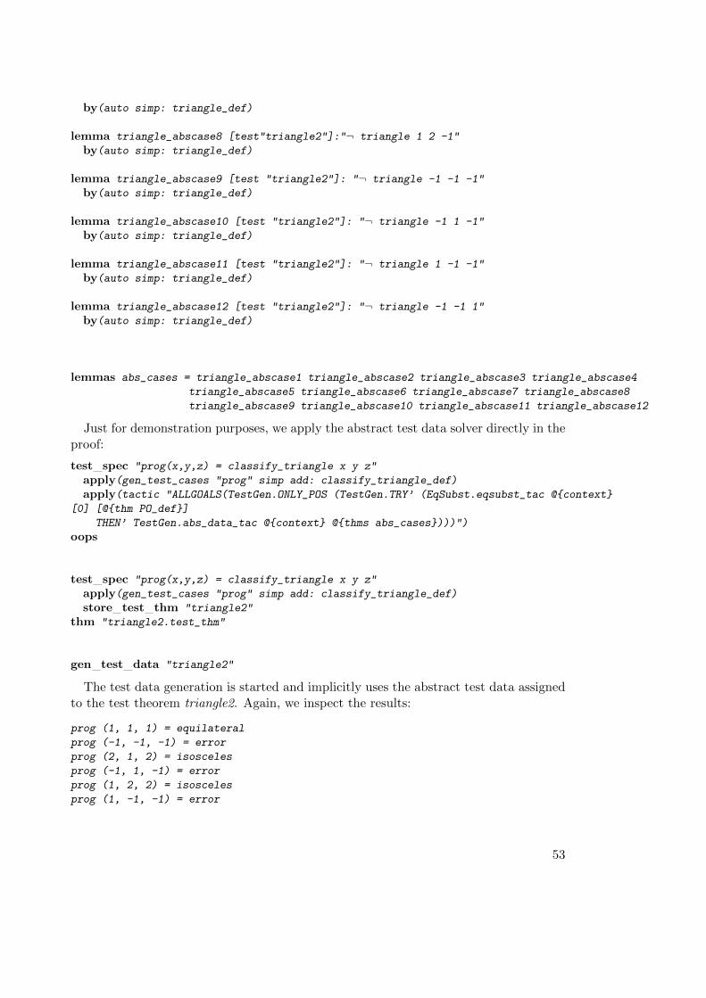
by(auto simp: triangle_def)
lemma triangle_abscase8 [test"triangle2"]:"¬ triangle 1 2 -1"
by(auto simp: triangle_def)
lemma triangle_abscase9 [test "triangle2"]: "¬ triangle -1 -1 -1"
by(auto simp: triangle_def)
lemma triangle_abscase10 [test "triangle2"]: "¬ triangle -1 1 -1"
by(auto simp: triangle_def)
lemma triangle_abscase11 [test "triangle2"]: "¬ triangle 1 -1 -1"
by(auto simp: triangle_def)
lemma triangle_abscase12 [test "triangle2"]: "¬ triangle -1 -1 1"
by(auto simp: triangle_def)
lemmas abs_cases = triangle_abscase1 triangle_abscase2 triangle_abscase3 triangle_abscase4
triangle_abscase5 triangle_abscase6 triangle_abscase7 triangle_abscase8
triangle_abscase9 triangle_abscase10 triangle_abscase11 triangle_abscase12
Just for demonstration purposes, we apply the abstract test data solver directly in theproof:
test spec "prog(x,y,z) = classify_triangle x y z"
apply(gen_test_cases "prog" simp add: classify_triangle_def)
apply(tactic "ALLGOALS(TestGen.ONLY_POS (TestGen.TRY’ (EqSubst.eqsubst_tac @{context}
[0] [@{thm PO_def}]
THEN’ TestGen.abs_data_tac @{context} @{thms abs_cases})))")
oops
test spec "prog(x,y,z) = classify_triangle x y z"
apply(gen_test_cases "prog" simp add: classify_triangle_def)
store test thm "triangle2"
thm "triangle2.test_thm"
gen test data "triangle2"
The test data generation is started and implicitly uses the abstract test data assignedto the test theorem triangle2. Again, we inspect the results:
prog (1, 1, 1) = equilateral
prog (-1, -1, -1) = error
prog (2, 1, 2) = isosceles
prog (-1, 1, -1) = error
prog (1, 2, 2) = isosceles
prog (1, -1, -1) = error
53
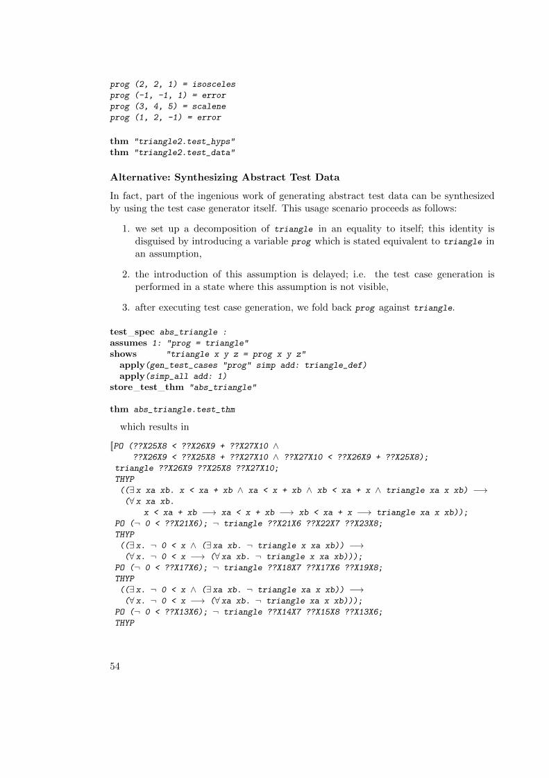
prog (2, 2, 1) = isosceles
prog (-1, -1, 1) = error
prog (3, 4, 5) = scalene
prog (1, 2, -1) = error
thm "triangle2.test_hyps"
thm "triangle2.test_data"
Alternative: Synthesizing Abstract Test Data
In fact, part of the ingenious work of generating abstract test data can be synthesizedby using the test case generator itself. This usage scenario proceeds as follows:
1. we set up a decomposition of triangle in an equality to itself; this identity isdisguised by introducing a variable prog which is stated equivalent to triangle inan assumption,
2. the introduction of this assumption is delayed; i.e. the test case generation isperformed in a state where this assumption is not visible,
3. after executing test case generation, we fold back prog against triangle.
test spec abs_triangle :
assumes 1: "prog = triangle"
shows "triangle x y z = prog x y z"
apply(gen_test_cases "prog" simp add: triangle_def)
apply(simp_all add: 1)
store test thm "abs_triangle"
thm abs_triangle.test_thm
which results in
[[PO (??X25X8 < ??X26X9 + ??X27X10 ∧??X26X9 < ??X25X8 + ??X27X10 ∧ ??X27X10 < ??X26X9 + ??X25X8);
triangle ??X26X9 ??X25X8 ??X27X10;
THYP
((∃ x xa xb. x < xa + xb ∧ xa < x + xb ∧ xb < xa + x ∧ triangle xa x xb) −→(∀ x xa xb.
x < xa + xb −→ xa < x + xb −→ xb < xa + x −→ triangle xa x xb));
PO (¬ 0 < ??X21X6); ¬ triangle ??X21X6 ??X22X7 ??X23X8;
THYP
((∃ x. ¬ 0 < x ∧ (∃ xa xb. ¬ triangle x xa xb)) −→(∀ x. ¬ 0 < x −→ (∀ xa xb. ¬ triangle x xa xb)));
PO (¬ 0 < ??X17X6); ¬ triangle ??X18X7 ??X17X6 ??X19X8;
THYP
((∃ x. ¬ 0 < x ∧ (∃ xa xb. ¬ triangle xa x xb)) −→(∀ x. ¬ 0 < x −→ (∀ xa xb. ¬ triangle xa x xb)));
PO (¬ 0 < ??X13X6); ¬ triangle ??X14X7 ??X15X8 ??X13X6;
THYP
54
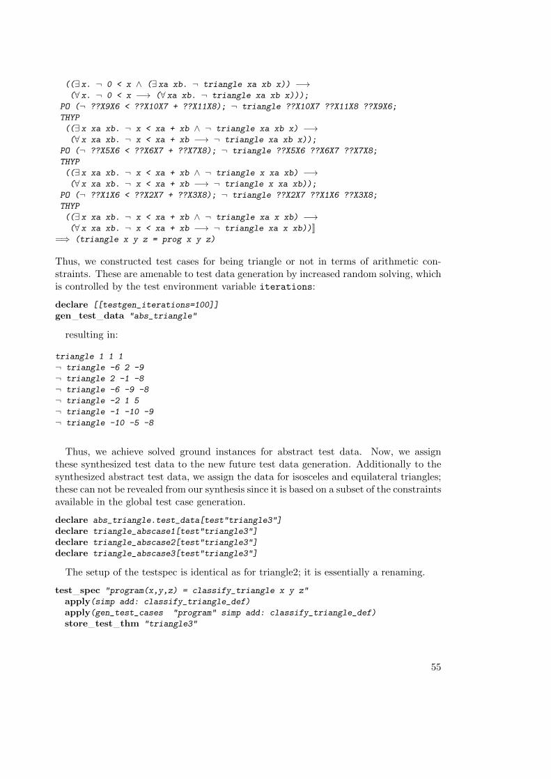
((∃ x. ¬ 0 < x ∧ (∃ xa xb. ¬ triangle xa xb x)) −→(∀ x. ¬ 0 < x −→ (∀ xa xb. ¬ triangle xa xb x)));
PO (¬ ??X9X6 < ??X10X7 + ??X11X8); ¬ triangle ??X10X7 ??X11X8 ??X9X6;
THYP
((∃ x xa xb. ¬ x < xa + xb ∧ ¬ triangle xa xb x) −→(∀ x xa xb. ¬ x < xa + xb −→ ¬ triangle xa xb x));
PO (¬ ??X5X6 < ??X6X7 + ??X7X8); ¬ triangle ??X5X6 ??X6X7 ??X7X8;
THYP
((∃ x xa xb. ¬ x < xa + xb ∧ ¬ triangle x xa xb) −→(∀ x xa xb. ¬ x < xa + xb −→ ¬ triangle x xa xb));
PO (¬ ??X1X6 < ??X2X7 + ??X3X8); ¬ triangle ??X2X7 ??X1X6 ??X3X8;
THYP
((∃ x xa xb. ¬ x < xa + xb ∧ ¬ triangle xa x xb) −→(∀ x xa xb. ¬ x < xa + xb −→ ¬ triangle xa x xb))]]
=⇒ (triangle x y z = prog x y z)
Thus, we constructed test cases for being triangle or not in terms of arithmetic con-straints. These are amenable to test data generation by increased random solving, whichis controlled by the test environment variable iterations:
declare [[testgen_iterations=100]]
gen test data "abs_triangle"
resulting in:
triangle 1 1 1
¬ triangle -6 2 -9
¬ triangle 2 -1 -8
¬ triangle -6 -9 -8
¬ triangle -2 1 5
¬ triangle -1 -10 -9
¬ triangle -10 -5 -8
Thus, we achieve solved ground instances for abstract test data. Now, we assignthese synthesized test data to the new future test data generation. Additionally to thesynthesized abstract test data, we assign the data for isosceles and equilateral triangles;these can not be revealed from our synthesis since it is based on a subset of the constraintsavailable in the global test case generation.
declare abs_triangle.test_data[test"triangle3"]
declare triangle_abscase1[test"triangle3"]
declare triangle_abscase2[test"triangle3"]
declare triangle_abscase3[test"triangle3"]
The setup of the testspec is identical as for triangle2; it is essentially a renaming.
test spec "program(x,y,z) = classify_triangle x y z"
apply(simp add: classify_triangle_def)
apply(gen_test_cases "program" simp add: classify_triangle_def)
store test thm "triangle3"
55

The test data generation is started again on the basis on synthesized and selectedhand-proven abstract data.
declare [[testgen_iterations=10]]
gen test data "triangle3"
thm "triangle3.test_hyps"
thm "triangle3.test_data"
end
6.3. Lists
theoryList_test
importsList
Testing
begin
In this example we present the current main application of HOL-TestGen: generatingtest data for black box testing of functional programs within a specification based unittest. We use a simple scenario, developing the test theory for testing sorting algorithmsover lists.
6.3.1. A Quick Walk Through
In the following we give a first impression of how the testing process using HOL-TestGenlooks like. For brevity we stick to default parameters and explain possible decision pointsand parameters where the testing can be improved in the next section.
Writing the Test Specification We start by specifying a primitive recursive predi-cate describing sorted lists:
primrec is_sorted:: "(’a::linorder) list ⇒ bool"
where "is_sorted [] = True" |
"is_sorted (x#xs) = (case xs of
[] ⇒ True
| y#ys ⇒ x ≤ y ∧ is_sorted xs)"
We will use this HOL predicate for describing our test specification, i.e. the propertiesour implementation should fulfill:
test spec "is_sorted(PUT (l::(’a list)))"
where PUT is a “placeholder” for our program under test.
56

Generating test cases Now we can automatically generate test cases. Using thedefault setup, we just apply our gen_test_cases :
apply(gen_test_cases "PUT")
which leads to the test partitioning one would expect:
1. is_sorted (PUT [])
2. is_sorted (PUT [??X8X3])
3. THYP ((∃ x. is_sorted (PUT [x])) −→ (∀ x. is_sorted (PUT [x])))
4. is_sorted (PUT [??X6X5, ??X5X4])
5. THYP
((∃ x xa. is_sorted (PUT [xa, x])) −→ (∀ x xa. is_sorted (PUT [xa, x])))
6. is_sorted (PUT [??X3X7, ??X2X6, ??X1X5])
7. THYP
((∃ x xa xb. is_sorted (PUT [xb, xa, x])) −→(∀ x xa xb. is_sorted (PUT [xb, xa, x])))
8. THYP (3 < length l −→ is_sorted (PUT l))
Now we bind the test theorem to a particular named test environment.
store test thm "is_sorted_result"
Generating test data Now we want to generate concrete test data, i.e. all variablesin the test cases must be instantiated with concrete values. This involves a randomsolver which tries to solve the constraints by randomly choosing values.
gen test data "is_sorted_result"
Which leads to the following test data:
is_sorted (PUT [])
is_sorted (PUT [-9])
is_sorted (PUT [-2, -2])
is_sorted (PUT [-1, 10, 3])
Note that by the following statements, the test data, the test hypotheses and the testtheorem can be inspected interactively.
thm is_sorted_result.test_data
thm is_sorted_result.test_hyps
thm is_sorted_result.test_thm
The generated test data can be exported to an external file:
export test data "list_data.dat" is_sorted_result
Mini-Example fun member :: "’a ⇒ ’a list ⇒ bool" ( infixl "mem" 50)
where"x mem S = False"
|"x mem (y # S) = (if x = y then True else x mem S)"
thm mem_def
57

Test Execution and Result Verification In principle, any SML-system should beable to run the provided test-harness and generated test-script. Using their specificfacilities for calling foreign code, testing of non-SML programs is possible. For example,one could test implementations written
• for the.Net platform, e.g., written in C# using sml.net [7],
• in C using, e.g. the foreign language interface of sml/NJ [6] or MLton [4],
• in Java using MLj [3].
Depending on the SML-system, the test execution can be done within an interpreter orusing a compiled test executable. Testing implementations written in SML is straight-forward, based on automatically generated test scripts. This generation is based on theinternal code generator of Isabelle and must be set up accordingly.
consts code "op <=" ("(_ <=/ _)")
The key command of the generation is:
which generates the following test harness:
(* ******************************************************************
* Test -Driver
* generated by HOL -TestGen 1.7.0 (dev: 8725:8750M)
****************************************************************** *)
structure TestDriver : sig end = struct
fun is_sorted [] = true
| is_sorted (x :: xs) =
(case xs of [] => true | (xa :: xb) => ((x <= xa) andalso is_sorted xs));
val return = ref ( [~6]:(( int list )));
fun eval x1 = let val ret = myList.sort x1 in (( return := ret);ret)end
fun retval () = SOME(! return );
fun toString a = (fn l => ("["^(List.foldr (fn (s1 ,s2)
=> (if s2 = "" then s1 else s1^", "^s2))
"" (map (fn x => Int.toString x) l))^"]")) a;
val testres = [];
val _ = print ("\nRunning Test Case 3:\n")
val pre_3 = [];
val post_3 = fn () => ( is_sorted (eval [~1, 10, 3]));
val res_3 = TestHarness.check retval pre_3 post_3;
val testres = testres@[res_3];
val _ = print ("\nRunning Test Case 2:\n")
val pre_2 = [];
58
val post_2 = fn () => ( is_sorted (eval [~2, ~2]));
val res_2 = TestHarness.check retval pre_2 post_2;
val testres = testres@[res_2];
val _ = print ("\nRunning Test Case 1:\n")
val pre_1 = [];
val post_1 = fn () => ( is_sorted (eval [~9]));
val res_1 = TestHarness.check retval pre_1 post_1;
val testres = testres@[res_1];
val _ = print ("\nRunning Test Case 0:\n")
val pre_0 = [];
val post_0 = fn () => ( is_sorted (eval []));
val res_0 = TestHarness.check retval pre_0 post_0;
val testres = testres@[res_0];
val _ = TestHarness.printList toString testres;
end
Further, suppose we have an ANSI C implementation of our sorting method for sortingC arrays that we want to test. Using the foreign language interface provided by theSML compiler MLton we first we have to import the sort method written in C using the_import keyword of MLton and further, we provide a “wrapper” doing some datatypeconversion, e.g. converting lists to arrays and vice versa:
structure myList = struct
val csort = _import "sort": int array * int -> int array;
fun toList a = Array.foldl (op ::) [] a;
fun sort l = toList(csort(Array.fromList(list),length l));
end
That’s all, now we can build the test executable using MLton and end up with a testexecutable which can be called directly. Running our test executable will result in thetest trace in Table 6.1 on the following page. Even this small set of test vectors issufficient to exploit an error in your implementation.
Improving the Testing Results
Obviously, in reality one would not be satisfied with the test cases generated in theprevious section: for testing sorting algorithms one would expect that the test datasomehow represents the set of permutations of the list elements. We have already seenthat the test specification used in the last section “only” enumerates lists up to a specificlength without any ordering constraints on their elements. Thus we decide to try amore ‘’descriptive” test specification that is based on the behavior of an insertion sortalgorithm:
fun ins :: "(’a::linorder) ⇒ ’a list ⇒ ’a list"
where "ins x [] = [x]"
59
Test Results:
=============
Test 0 - SUCCESS, result: []
Test 1 - SUCCESS, result: [10]
Test 2 - SUCCESS, result: [72, 42]
Test 3 - *** FAILURE: post-condition false, result: [8, 15, -31]
Summary:
--------
Number successful tests cases: 3 of 4 (ca. 75%)
Number of warnings: 0 of 4 (ca. 0%)
Number of errors: 0 of 4 (ca. 0%)
Number of failures: 1 of 4 (ca. 25%)
Number of fatal errors: 0 of 4 (ca. 0%)
Overall result: failed
===============
Table 6.1.: A Sample Test Trace
|"ins x (y#ys) = (if (x < y) then x#y#ys else (y#(ins x ys)))"
fun sort:: "(’a::linorder) list ⇒ ’a list"
where "sort [] = [] "
| "sort (x#xs) = ins x (sort xs)"
Now we state our test specification by requiring that the behavior of the programunder test PUT is identical to the behavior of our specified sorting algorithm sort :
Based on this specification gen_test_cases produces test cases representing all per-mutations of lists up to a fixed length n. Normally, we also want to configure up towhich length lists should be generated (we call this the depth of test case), e.g. we decideto generate lists up to length 3. Our standard setup
test spec "sort l = PUT l"
apply(gen_test_cases "PUT")
store test thm "is_sorting_algorithm0"
generates 9 test cases describing all permutations of lists of length 1, 2 and 3. ”Per-mutation” means here that not only test cases (i.e. I/O-partitions) are generated forlists of length 0, 1, 2 and 3; the partitioning is actually finer: for two-elementary lists,for example, the case of a list with the first element larger or equal and the dual caseare distinguished. The entire test-theorem looks as follows:
[[[] = PUT []; [??X31X3] = PUT [??X31X3]; THYP ((∃ x. [x] = PUT [x]) −→ (∀ x. [x]
= PUT [x])); PO (??X29X6 < ??X28X5); [??X29X6, ??X28X5] = PUT [??X29X6, ??X28X5];
THYP ((∃ x xa. xa < x ∧ [xa, x] = PUT [xa, x]) −→ (∀ x xa. xa < x −→ [xa, x] = PUT
[xa, x])); PO (¬ ??X26X6 < ??X25X5); [??X25X5, ??X26X6] = PUT [??X26X6, ??X25X5];
THYP ((∃ x xa. ¬ xa < x ∧ [x, xa] = PUT [xa, x]) −→ (∀ x xa. ¬ xa < x −→ [x, xa]
60
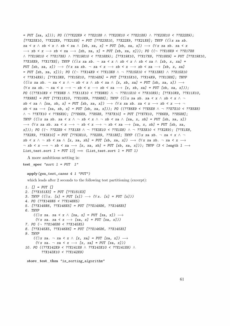
= PUT [xa, x])); PO ((??X22X9 < ??X21X8 ∧ ??X23X10 < ??X21X8) ∧ ??X23X10 < ??X22X9);
[??X23X10, ??X22X9, ??X21X8] = PUT [??X23X10, ??X22X9, ??X21X8]; THYP ((∃ x xa xb.
xa < x ∧ xb < x ∧ xb < xa ∧ [xb, xa, x] = PUT [xb, xa, x]) −→ (∀ x xa xb. xa < x
−→ xb < x −→ xb < xa −→ [xb, xa, x] = PUT [xb, xa, x])); PO ((¬ ??X18X9 < ??X17X8
∧ ??X19X10 < ??X17X8) ∧ ??X19X10 < ??X18X9); [??X19X10, ??X17X8, ??X18X9] = PUT [??X19X10,
??X18X9, ??X17X8]; THYP ((∃ x xa xb. ¬ xa < x ∧ xb < x ∧ xb < xa ∧ [xb, x, xa] =
PUT [xb, xa, x]) −→ (∀ x xa xb. ¬ xa < x −→ xb < x −→ xb < xa −→ [xb, x, xa]
= PUT [xb, xa, x])); PO ((¬ ??X14X9 < ??X13X8 ∧ ¬ ??X15X10 < ??X13X8) ∧ ??X15X10
< ??X14X9); [??X13X8, ??X15X10, ??X14X9] = PUT [??X15X10, ??X14X9, ??X13X8]; THYP
((∃ x xa xb. ¬ xa < x ∧ ¬ xb < x ∧ xb < xa ∧ [x, xb, xa] = PUT [xb, xa, x]) −→(∀ x xa xb. ¬ xa < x −→ ¬ xb < x −→ xb < xa −→ [x, xb, xa] = PUT [xb, xa, x]));
PO ((??X10X9 < ??X9X8 ∧ ??X11X10 < ??X9X8) ∧ ¬ ??X11X10 < ??X10X9); [??X10X9, ??X11X10,
??X9X8] = PUT [??X11X10, ??X10X9, ??X9X8]; THYP ((∃ x xa xb. xa < x ∧ xb < x ∧ ¬xb < xa ∧ [xa, xb, x] = PUT [xb, xa, x]) −→ (∀ x xa xb. xa < x −→ xb < x −→ ¬xb < xa −→ [xa, xb, x] = PUT [xb, xa, x])); PO ((??X6X9 < ??X5X8 ∧ ¬ ??X7X10 < ??X5X8)
∧ ¬ ??X7X10 < ??X6X9); [??X6X9, ??X5X8, ??X7X10] = PUT [??X7X10, ??X6X9, ??X5X8];
THYP ((∃ x xa xb. xa < x ∧ ¬ xb < x ∧ ¬ xb < xa ∧ [xa, x, xb] = PUT [xb, xa, x])
−→ (∀ x xa xb. xa < x −→ ¬ xb < x −→ ¬ xb < xa −→ [xa, x, xb] = PUT [xb, xa,
x])); PO ((¬ ??X2X9 < ??X1X8 ∧ ¬ ??X3X10 < ??X1X8) ∧ ¬ ??X3X10 < ??X2X9); [??X1X8,
??X2X9, ??X3X10] = PUT [??X3X10, ??X2X9, ??X1X8]; THYP ((∃ x xa xb. ¬ xa < x ∧ ¬xb < x ∧ ¬ xb < xa ∧ [x, xa, xb] = PUT [xb, xa, x]) −→ (∀ x xa xb. ¬ xa < x −→¬ xb < x −→ ¬ xb < xa −→ [x, xa, xb] = PUT [xb, xa, x])); THYP (3 < length l −→List_test.sort l = PUT l)]] =⇒ (List_test.sort l = PUT l)
A more ambitious setting is:
test spec "sort l = PUT l"
apply(gen_test_cases 4 1 "PUT")
which leads after 2 seconds to the following test partitioning (excerpt):
1. [] = PUT []
2. [??X151X3] = PUT [??X151X3]
3. THYP ((∃ x. [x] = PUT [x]) −→ (∀ x. [x] = PUT [x]))
4. PO (??X149X6 < ??X148X5)
5. [??X149X6, ??X148X5] = PUT [??X149X6, ??X148X5]
6. THYP
((∃ x xa. xa < x ∧ [xa, x] = PUT [xa, x]) −→(∀ x xa. xa < x −→ [xa, x] = PUT [xa, x]))
7. PO (¬ ??X146X6 < ??X145X5)
8. [??X145X5, ??X146X6] = PUT [??X146X6, ??X145X5]
9. THYP
((∃ x xa. ¬ xa < x ∧ [x, xa] = PUT [xa, x]) −→(∀ x xa. ¬ xa < x −→ [x, xa] = PUT [xa, x]))
10. PO ((??X142X9 < ??X141X8 ∧ ??X143X10 < ??X141X8) ∧??X143X10 < ??X142X9)
store test thm "is_sorting_algorithm"
61
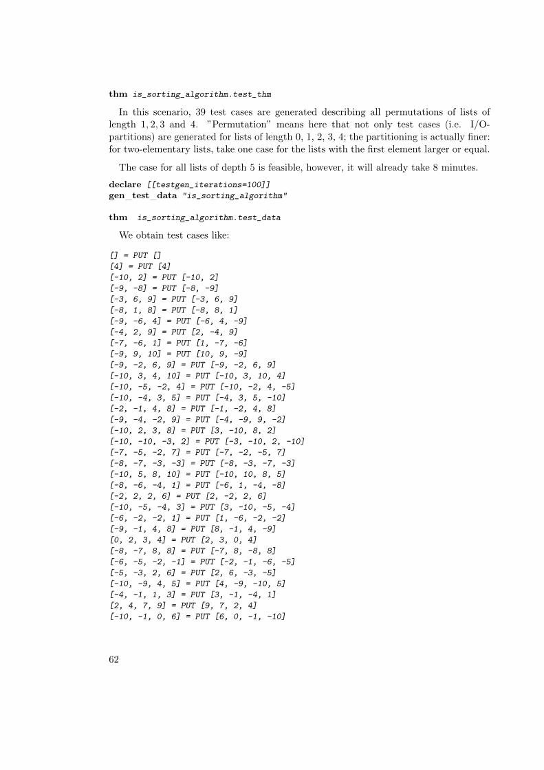
thm is_sorting_algorithm.test_thm
In this scenario, 39 test cases are generated describing all permutations of lists oflength 1, 2, 3 and 4. ”Permutation” means here that not only test cases (i.e. I/O-partitions) are generated for lists of length 0, 1, 2, 3, 4; the partitioning is actually finer:for two-elementary lists, take one case for the lists with the first element larger or equal.
The case for all lists of depth 5 is feasible, however, it will already take 8 minutes.
declare [[testgen_iterations=100]]
gen test data "is_sorting_algorithm"
thm is_sorting_algorithm.test_data
We obtain test cases like:
[] = PUT []
[4] = PUT [4]
[-10, 2] = PUT [-10, 2]
[-9, -8] = PUT [-8, -9]
[-3, 6, 9] = PUT [-3, 6, 9]
[-8, 1, 8] = PUT [-8, 8, 1]
[-9, -6, 4] = PUT [-6, 4, -9]
[-4, 2, 9] = PUT [2, -4, 9]
[-7, -6, 1] = PUT [1, -7, -6]
[-9, 9, 10] = PUT [10, 9, -9]
[-9, -2, 6, 9] = PUT [-9, -2, 6, 9]
[-10, 3, 4, 10] = PUT [-10, 3, 10, 4]
[-10, -5, -2, 4] = PUT [-10, -2, 4, -5]
[-10, -4, 3, 5] = PUT [-4, 3, 5, -10]
[-2, -1, 4, 8] = PUT [-1, -2, 4, 8]
[-9, -4, -2, 9] = PUT [-4, -9, 9, -2]
[-10, 2, 3, 8] = PUT [3, -10, 8, 2]
[-10, -10, -3, 2] = PUT [-3, -10, 2, -10]
[-7, -5, -2, 7] = PUT [-7, -2, -5, 7]
[-8, -7, -3, -3] = PUT [-8, -3, -7, -3]
[-10, 5, 8, 10] = PUT [-10, 10, 8, 5]
[-8, -6, -4, 1] = PUT [-6, 1, -4, -8]
[-2, 2, 2, 6] = PUT [2, -2, 2, 6]
[-10, -5, -4, 3] = PUT [3, -10, -5, -4]
[-6, -2, -2, 1] = PUT [1, -6, -2, -2]
[-9, -1, 4, 8] = PUT [8, -1, 4, -9]
[0, 2, 3, 4] = PUT [2, 3, 0, 4]
[-8, -7, 8, 8] = PUT [-7, 8, -8, 8]
[-6, -5, -2, -1] = PUT [-2, -1, -6, -5]
[-5, -3, 2, 6] = PUT [2, 6, -3, -5]
[-10, -9, 4, 5] = PUT [4, -9, -10, 5]
[-4, -1, 1, 3] = PUT [3, -1, -4, 1]
[2, 4, 7, 9] = PUT [9, 7, 2, 4]
[-10, -1, 0, 6] = PUT [6, 0, -1, -10]
62
If we scale down to only 10 iterations, this is not sufficient to solve all conditions, i.e.we obtain many test cases with unresolved constraints where RSF marks unsolved cases.In these cases, it is unclear if the test partition is empty. Analyzing the generated testdata reveals that all cases for lists with length up to (and including) 3 could be solved.From the 24 cases for lists of length 4 only 9 could be solved by the random solver (thus,overall 19 of the 34 cases were solved). To achieve better results, we could interactivelyincrease the number of iterations which reveals that we need to set iterations to 100 tofind all solutions reliably.
iterations 5 10 20 25 30 40 50 75 100
solved goals (of 34) 13 19 23 24 25 29 33 33 34
Instead of increasing the number of iterations one could also add other techniques suchas
1. deriving new rules that allow for the generation of a simplified test theorem,
2. introducing abstract test cases or
3. supporting the solving process by derived rules.
Non-Inherent Higher-order Testing
HOL-TestGen can use test specifications that contain higher-order operators — althoughwe would not claim that the test case generation is actually higher-order (there are noenumeration schemes for the function space, so function variables are untreated by thetest case generation procedure so far).
Just for fun, we reformulate the problem of finding the maximal number in a list as ahigher-order problem:
test spec " foldr max l (0::int) = PUT l"
apply(gen_test_cases "PUT" simp:max_def)
store test thm "maximal_number"
Now the test data:
declare [[testgen_iterations=200]]
gen test data "maximal_number"
thm maximal_number.test_data
end
6.3.2. Test and Verification
theoryList_Verified_test
63
importsList
Testing
begin
We repeat our standard List example and verify the resulting test-hypothesis wrt. toa implementation given after the black-box test-case generation.
The example sheds some light one the nature of test vs. verification.
Writing the Test Specification
We start by specifying a primitive recursive predicate describing sorted lists:
fun is_sorted:: "(’a::ord) list ⇒ bool"
where "is_sorted [] = True"
| "is_sorted (x#xs) = ((case xs of [] ⇒ True
| y#ys ⇒ (x < y) ∨ (x = y))
∧ is_sorted xs)"
Generating test cases
Now we can automatically generate test cases. Using the default setup, we just applyour gen_test_cases on the free variable PUT (for program under test):
test spec "is_sorted(PUT (l::(’a list)))"
apply(gen_test_cases PUT)
which leads to the test partitioning one would expect:
1. is_sorted (PUT [])
2. is_sorted (PUT [??X8X3])
3. THYP ((∃ x. is_sorted (PUT [x])) −→ (∀ x. is_sorted (PUT [x])))
4. is_sorted (PUT [??X6X5, ??X5X4])
5. THYP
((∃ x xa. is_sorted (PUT [xa, x])) −→ (∀ x xa. is_sorted (PUT [xa, x])))
6. is_sorted (PUT [??X3X7, ??X2X6, ??X1X5])
7. THYP
((∃ x xa xb. is_sorted (PUT [xb, xa, x])) −→(∀ x xa xb. is_sorted (PUT [xb, xa, x])))
8. THYP (3 < length l −→ is_sorted (PUT l))
Now we bind the test theorem to a particular named test environment.
store test thm "test_sorting"
gen test data "test_sorting"
Note that by the following statements, the test data, the test hypotheses and the testtheorem can be inspected interactively.
thm test_sorting.test_data
thm test_sorting.test_hyps
thm test_sorting.test_thm
64
In this example, we will have a closer look on the test-hypotheses:
THYP ((∃ x. is_sorted (PUT [x])) −→ (∀ x. is_sorted (PUT [x])))
THYP ((∃ x xa. is_sorted (PUT [xa, x])) −→ (∀ x xa. is_sorted (PUT [xa, x])))
THYP
((∃ x xa xb. is_sorted (PUT [xb, xa, x])) −→(∀ x xa xb. is_sorted (PUT [xb, xa, x])))
THYP (3 < length l −→ is_sorted (PUT l))
Linking Tests and Uniformity
The uniformity hypotheses and the tests establish together the fact:
lemma uniformity_vs_separation:
assumes test_0: "is_sorted (PUT [])"
assumes test_1: "EX (x::(’a::linorder)). is_sorted (PUT [x])"
assumes test_2: "EX (x::(’a::linorder)) xa. is_sorted (PUT [xa, x])"
assumes test_3: "EX (x::(’a::linorder)) xa xaa. is_sorted (PUT [xaa, xa, x])"
assumes thyp_uniform_1:"THYP ((EX (x::(’a::linorder)). is_sorted (PUT [x])) −→
(ALL (x::(’a::linorder)). is_sorted (PUT [x])))"
assumes thyp_uniform_2:"THYP ((EX (x::(’a::linorder)) xa. is_sorted (PUT [xa, x]))
−→(ALL (x::(’a::linorder)) xa. is_sorted (PUT [xa, x])))"
assumes thyp_uniform_3:"THYP ((EX (x::(’a::linorder)) xa xaa. is_sorted (PUT [xaa,
xa, x])) −→(ALL (x::(’a::linorder)) xa xaa. is_sorted (PUT [xaa,
xa, x])))"
shows "ALL (l::(’a::linorder)list). length l ≤ 3 −→ is_sorted (PUT l)"
apply(insert thyp_uniform_1 thyp_uniform_2 thyp_uniform_3)
apply(simp only: test_1 test_2 test_3 THYP_def)
apply safe
apply(rule_tac y=l in list.exhaust,simp add: test_0)
apply(rule_tac y=list in list.exhaust,simp)
apply(rule_tac y=lista in list.exhaust,simp)
apply(hypsubst,simp)done
This means that if the provided tests are successful and all uniformity hypotheseshold, the test specification holds up to measure 3. Note that this is a universal factindependent from any implementation.
Giving a Program and verifying the Test Hypotheses for it.
In the following, we give an instance for PUT in form of the usual insertion sort algorithm.Thus, we turn the black-box scenario into a white-box scenario.
primrec ins :: "[’a::linorder, ’a list] ⇒ ’a list "
where "ins x [] = [x]" |
65

"ins x (y#ys) = (if (x < y) then x#(ins y ys) else (y#(ins x ys)))"
primrec sort :: "(’a::linorder) list ⇒ ’a list"
where "sort [] = []" |
"sort (x#xs) = ins x (sort xs)"
thm test_sorting.test_hyps
lemma uniform_1:
"THYP ((EX x. is_sorted (sort [x])) −→ (ALL x. is_sorted (sort [x])))"
by(auto simp:THYP_def)
lemma uniform_2:
"THYP ((EX x xa. is_sorted (sort [xa, x])) −→ (ALL x xa. is_sorted (sort [xa, x])))"
by(auto simp:THYP_def)
A Proof in Slow-Motion:
lemma uniform_2_b:
"THYP ((EX x xa. is_sorted (sort [xa, x])) −→ (ALL x xa. is_sorted (sort [xa, x])))"
apply(simp only: THYP_def)
apply(rule impI, thin_tac "?X")
apply(rule allI)+
We reduce the test-hypothesis to the core and get:
1.∧x xa. is_sorted (List_Verified_test.sort [xa, x])
. Unfolding sort yields:
apply(simp only: sort.simps)
1.∧x xa. is_sorted (ins xa (ins x []))
and after unfolding of ins we get:
apply(simp only: ins.simps)
1.∧x xa. is_sorted (if xa < x then [xa, x] else [x, xa])
Case-splitting results in:
apply(case_tac "xa < x", simp_all only: if_True if_False)
1.∧x xa. xa < x =⇒ is_sorted [xa, x]
2.∧x xa. ¬ xa < x =⇒ is_sorted [x, xa]
Evaluation of is_sorted yields:
apply(simp_all only: is_sorted.simps)
66
1.∧x xa.
xa < x =⇒(case [x] of [] ⇒ True | y # ys ⇒ xa < y ∨ xa = y) ∧(case [] of [] ⇒ True | y # ys ⇒ x < y ∨ x = y) ∧ True
2.∧x xa.
¬ xa < x =⇒(case [xa] of [] ⇒ True | y # ys ⇒ x < y ∨ x = y) ∧(case [] of [] ⇒ True | y # ys ⇒ xa < y ∨ xa = y) ∧ True
which can be reduced to:
apply(simp_all)
1.∧x xa. ¬ xa < x =⇒ x < xa ∨ x = xa
which results by arithmetic reasoning to True.
apply(auto)done
The proof reveals that the test is in fact irrelevant for the proof - the core is thecase-distinction over all possible orderings of lists of length 2; what we check is thatis_sorted exactly fits to sort.
lemma uniform_3:
"THYP ((EX x xa xaa. is_sorted (sort [xaa, xa, x])) −→(ALL x xa xaa. is_sorted (sort [xaa, xa, x])))"
The standard automated approach:
apply(auto simp:THYP_def)
does (probably) not terminate due to mini - scoping. Instead, the following tactical proof exploitsthe structure of the uniformity hypothesis directly and leads to easily automated verification. Itshould still work for substantially larger test specifications.
apply(simp only: THYP_def)
apply(rule impI,(erule exE)+,(rule allI)+)
apply auto
done
lemma is_sorted_invariant_ins[rule_format]:
"is_sorted l −→ is_sorted (ins a l)"
apply(induct l)
apply(auto)apply(rule_tac y=l in list.exhaust, simp,auto)
apply(rule_tac y=l in list.exhaust, auto)
apply(rule_tac y=list in list.exhaust, auto)
apply(subgoal_tac "a < aaa",simp)
apply(erule Orderings.xtrans(10),simp)
67
apply(rule_tac y=list in list.exhaust, auto)
apply(rule_tac y=l in list.exhaust, auto)
done
lemma testspec_proven: "is_sorted (sort l)"
by(induct l,simp_all,erule is_sorted_invariant_ins)
Well, that’s not too exciting, having is_sorted_invariant_ins.
Now we establish the same facts over tests.
lemma test_1: "is_sorted (sort [])" by auto
lemma test_2: "is_sorted (sort [1::int])" by auto
lemma test_3: "is_sorted (sort [1::int, 7])" by auto
lemma test_4: "is_sorted (sort [6::int, 4, 9])" by auto
Now we establish the data-separation for the concrete implementation sort:
lemma separation_for_sort:
"ALL l::int list. length l ≤ 3 −→ is_sorted (sort l)"
apply(rule uniformity_vs_separation)
apply(rule test_1)
apply((rule exI)+,((rule test_2) | (rule test_3) | (rule test_4)))+
apply(rule uniform_1, rule uniform_2, rule uniform_3)
done
lemma regularity_over_local_test:
"THYP (3 < length (l::int list) −→ is_sorted (sort l))"
proof -
have anchor : "∧a l. length (l:: int list) = 3 =⇒ is_sorted (ins a (sort l))"
apply(auto intro!: separation_for_sort[THEN spec,THEN mp] is_sorted_invariant_ins)
donehave step : "
∧a l. is_sorted (sort (l:: int list)) =⇒ is_sorted (ins a (sort
l))"
apply(erule is_sorted_invariant_ins)
doneshow ?thesis
apply(simp only: THYP_def)
1. 3 < length l −→ is_sorted (List_Verified_test.sort l)
apply(induct l, auto)
1.∧a l. [[2 < length l; ¬ 3 < length l]]
=⇒ is_sorted (ins a (List_Verified_test.sort l))
2.∧a l. [[2 < length l; is_sorted (List_Verified_test.sort l)]]
=⇒ is_sorted (ins a (List_Verified_test.sort l))
68
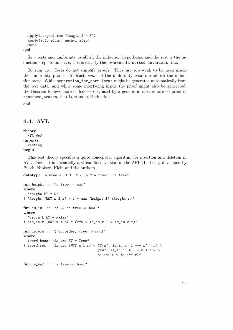
apply(subgoal_tac "length l = 3")
apply(auto elim!: anchor step)
doneqed
So – tests and uniformity establish the induction hypothesis, and the rest is the in-duction step. In our case, this is exactly the invariant is_sorted_invariant_ins.
To sum up : Tests do not simplify proofs. They are too weak to be used insidethe uniformity proofs. At least, some of the uniformity results establish the induc-tion steps. While separation_for_sort lemma might be generated automatically fromthe test data, and while some interfacing inside the proof might also be generated,the theorem follows more or less — disguised by a generic infra-structure — proof oftestspec_proven, that is, standard induction.
end
6.4. AVL
theoryAVL_def
importsTesting
begin
This test theory specifies a quite conceptual algorithm for insertion and deletion inAVL Trees. It is essentially a streamlined version of the AFP [1] theory developed byPusch, Nipkow, Klein and the authors.
datatype ’a tree = ET | MKT ’a "’a tree" "’a tree"
fun height :: "’a tree ⇒ nat"
where"height ET = 0"
| "height (MKT n l r) = 1 + max (height l) (height r)"
fun is_in :: "’a ⇒ ’a tree ⇒ bool"
where"is_in k ET = False"
| "is_in k (MKT n l r) = (k=n ∨ is_in k l ∨ is_in k r)"
fun is_ord :: "(’a::order) tree ⇒ bool"
whereisord_base: "is_ord ET = True"
| isord_rec: "is_ord (MKT n l r) = ((∀ n’. is_in n’ l −→ n’ < n) ∧(∀ n’. is_in n’ r −→ n < n’) ∧is_ord l ∧ is_ord r)"
fun is_bal :: "’a tree ⇒ bool"
69

where"is_bal ET = True"
| "is_bal (MKT n l r) = ((height l = height r ∨height l = 1+height r ∨height r = 1+height l) ∧is_bal l ∧ is_bal r)"
We also provide a more efficient variant of is_in :
funis_in_eff :: "(’a::order) ⇒ ’a tree ⇒ bool"
where"is_in_eff k ET = False"
| "is_in_eff k (MKT n l r) = (if k = n then True
else (if k<n then (is_in_eff k l)
else (is_in_eff k r)))"
datatype bal = Just | Left | Right
definition bal :: "’a tree ⇒ bal"
where "bal t ≡ case t of ET ⇒ Just
| (MKT n l r) ⇒ if height l = height r then Just
else if height l < height r then Right
else Left"
hide const ln
fun r_rot :: "’a × ’a tree × ’a tree ⇒ ’a tree"
where "r_rot (n, MKT ln ll lr, r) = MKT ln ll (MKT n lr r)"
fun l_rot :: "’a × ’a tree × ’a tree ⇒ ’a tree"
where "l_rot(n, l, MKT rn rl rr) = MKT rn (MKT n l rl) rr"
fun lr_rot :: "’a × ’a tree × ’a tree ⇒ ’a tree"
where "lr_rot(n, MKT ln ll (MKT lrn lrl lrr), r) =
MKT lrn (MKT ln ll lrl) (MKT n lrr r)"
fun rl_rot :: "’a × ’a tree × ’a tree ⇒ ’a tree"
where "rl_rot(n, l, MKT rn (MKT rln rll rlr) rr) =
MKT rln (MKT n l rll) (MKT rn rlr rr)"
definition l_bal :: "’a ⇒ ’a tree ⇒ ’a tree ⇒ ’a tree"
where "l_bal n l r ≡ if bal l = Right
then lr_rot (n, l, r)
else r_rot (n, l, r)"
definition r_bal :: "’a ⇒ ’a tree ⇒ ’a tree ⇒ ’a tree"
where "r_bal n l r ≡ if bal r = Left
then rl_rot (n, l, r)
70
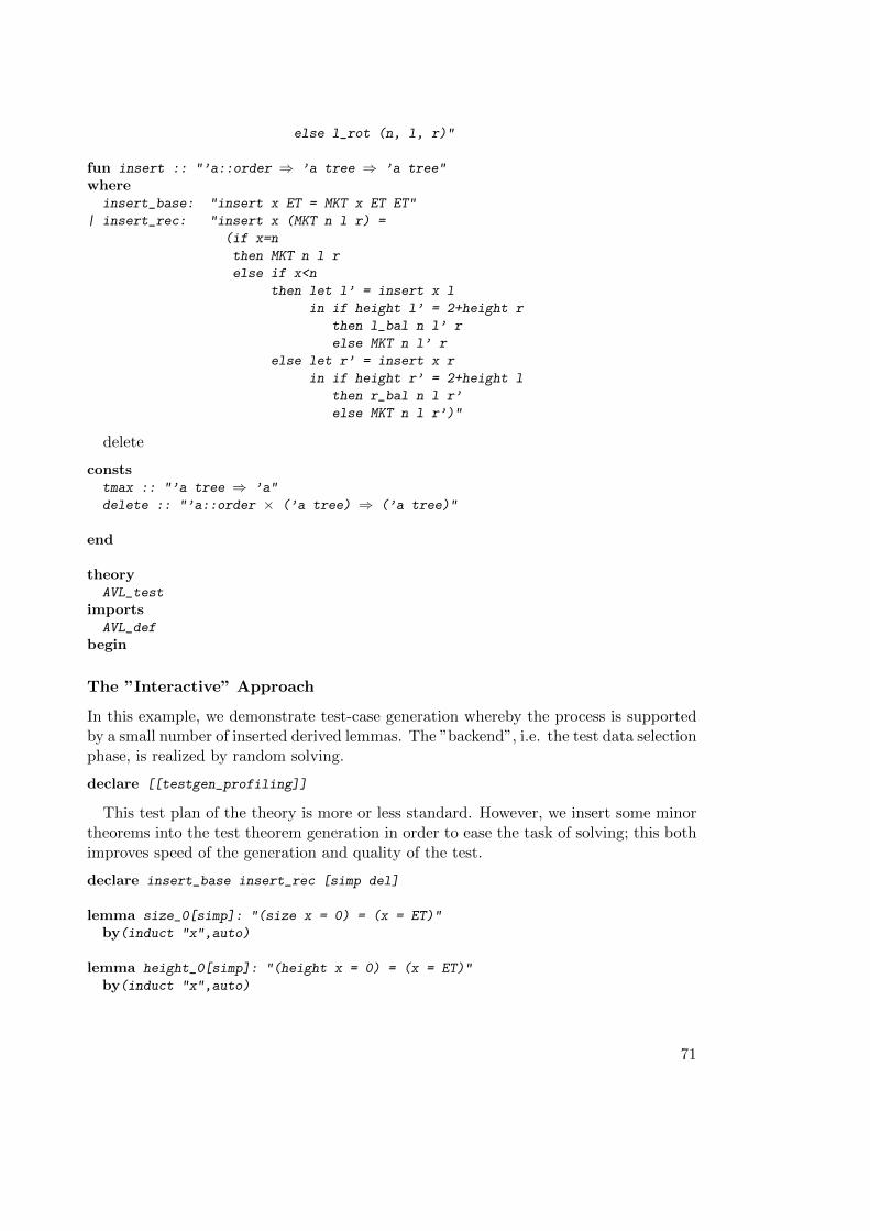
else l_rot (n, l, r)"
fun insert :: "’a::order ⇒ ’a tree ⇒ ’a tree"
whereinsert_base: "insert x ET = MKT x ET ET"
| insert_rec: "insert x (MKT n l r) =
(if x=n
then MKT n l r
else if x<n
then let l’ = insert x l
in if height l’ = 2+height r
then l_bal n l’ r
else MKT n l’ r
else let r’ = insert x r
in if height r’ = 2+height l
then r_bal n l r’
else MKT n l r’)"
delete
conststmax :: "’a tree ⇒ ’a"
delete :: "’a::order × (’a tree) ⇒ (’a tree)"
end
theoryAVL_test
importsAVL_def
begin
The ”Interactive” Approach
In this example, we demonstrate test-case generation whereby the process is supportedby a small number of inserted derived lemmas. The ”backend”, i.e. the test data selectionphase, is realized by random solving.
declare [[testgen_profiling]]
This test plan of the theory is more or less standard. However, we insert some minortheorems into the test theorem generation in order to ease the task of solving; this bothimproves speed of the generation and quality of the test.
declare insert_base insert_rec [simp del]
lemma size_0[simp]: "(size x = 0) = (x = ET)"
by(induct "x",auto)
lemma height_0[simp]: "(height x = 0) = (x = ET)"
by(induct "x",auto)
71
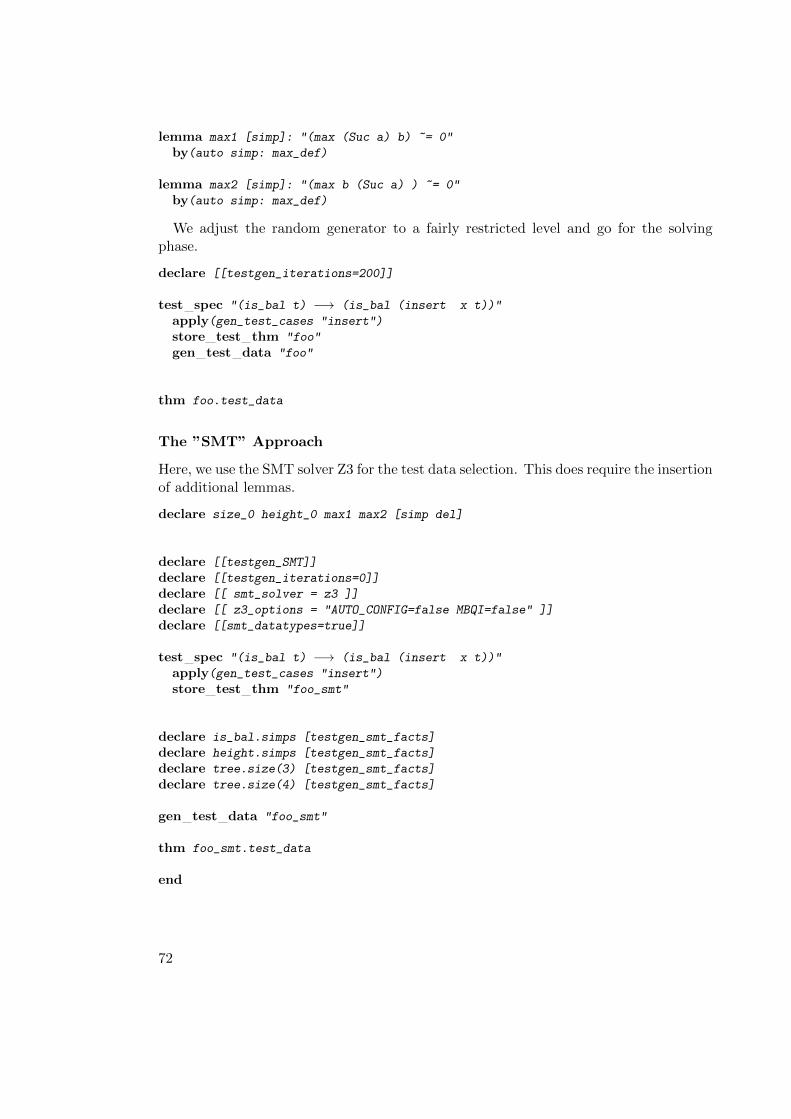
lemma max1 [simp]: "(max (Suc a) b) ~= 0"
by(auto simp: max_def)
lemma max2 [simp]: "(max b (Suc a) ) ~= 0"
by(auto simp: max_def)
We adjust the random generator to a fairly restricted level and go for the solvingphase.
declare [[testgen_iterations=200]]
test spec "(is_bal t) −→ (is_bal (insert x t))"
apply(gen_test_cases "insert")
store test thm "foo"
gen test data "foo"
thm foo.test_data
The ”SMT” Approach
Here, we use the SMT solver Z3 for the test data selection. This does require the insertionof additional lemmas.
declare size_0 height_0 max1 max2 [simp del]
declare [[testgen_SMT]]
declare [[testgen_iterations=0]]
declare [[ smt_solver = z3 ]]
declare [[ z3_options = "AUTO_CONFIG=false MBQI=false" ]]
declare [[smt_datatypes=true]]
test spec "(is_bal t) −→ (is_bal (insert x t))"
apply(gen_test_cases "insert")
store test thm "foo_smt"
declare is_bal.simps [testgen_smt_facts]
declare height.simps [testgen_smt_facts]
declare tree.size(3) [testgen_smt_facts]
declare tree.size(4) [testgen_smt_facts]
gen test data "foo_smt"
thm foo_smt.test_data
end
72
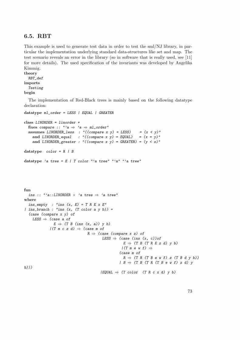
6.5. RBT
This example is used to generate test data in order to test the sml/NJ library, in par-ticular the implementation underlying standard data-structures like set and map. Thetest scenario reveals an error in the library (so in software that is really used, see [11]for more details). The used specification of the invariants was developed by AngelikaKimmig.theoryRBT_def
importsTesting
begin
The implementation of Red-Black trees is mainly based on the following datatypedeclaration:
datatype ml_order = LESS | EQUAL | GREATER
class LINORDER = linorder +
fixes compare :: "’a ⇒ ’a ⇒ ml_order"
assumes LINORDER_less : "((compare x y) = LESS) = (x < y)"
and LINORDER_equal : "((compare x y) = EQUAL) = (x = y)"
and LINORDER_greater : "((compare x y) = GREATER) = (y < x)"
datatype color = R | B
datatype ’a tree = E | T color "’a tree" "’a" "’a tree"
funins :: "’a::LINORDER × ’a tree ⇒ ’a tree"
whereins_empty : "ins (x, E) = T R E x E"
| ins_branch : "ins (x, (T color a y b)) =
(case (compare x y) of
LESS ⇒ (case a of
E ⇒ (T B (ins (x, a)) y b)
|(T m c z d) ⇒ (case m of
R ⇒ (case (compare x z) of
LESS ⇒ (case (ins (x, c))of
E ⇒ (T B (T R E z d) y b)
|(T m e w f) ⇒(case m of
R ⇒ (T R (T B e w f) z (T B d y b))
| B ⇒ (T B (T R (T B e w f) z d) y
b)))
|EQUAL ⇒ (T color (T R c x d) y b)
73
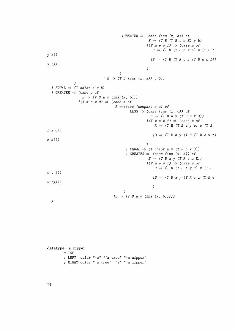
|GREATER ⇒ (case (ins (x, d)) of
E ⇒ (T B (T R c z E) y b)
|(T m e w f) ⇒ (case m of
R ⇒ (T R (T B c z e) w (T B f
y b))
|B ⇒ (T B (T R c z (T B e w f))
y b))
)
)
| B ⇒ (T B (ins (x, a)) y b))
)
| EQUAL ⇒ (T color a x b)
| GREATER ⇒ (case b of
E ⇒ (T B a y (ins (x, b)))
|(T m c z d) ⇒ (case m of
R ⇒(case (compare x z) of
LESS ⇒ (case (ins (x, c)) of
E ⇒ (T B a y (T R E z d))
|(T m e w f) ⇒ (case m of
R ⇒ (T R (T B a y e) w (T B
f z d))
|B ⇒ (T B a y (T R (T B e w f)
z d)))
)
| EQUAL ⇒ (T color a y (T R c x d))
| GREATER ⇒ (case (ins (x, d)) of
E ⇒ (T B a y (T R c z E))
|(T m e w f) ⇒ (case m of
R ⇒ (T R (T B a y c) z (T B
e w f))
|B ⇒ (T B a y (T R c z (T B e
w f))))
)
)
|B ⇒ (T B a y (ins (x, b)))))
)"
datatype ’a zipper
= TOP
| LEFT color "’a" "’a tree" "’a zipper"
| RIGHT color "’a tree" "’a" "’a zipper"
74
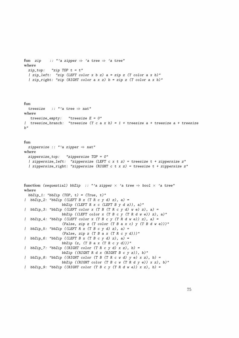
fun zip :: "’a zipper ⇒ ’a tree ⇒ ’a tree"
wherezip_top: "zip TOP t = t"
| zip_left: "zip (LEFT color x b z) a = zip z (T color a x b)"
| zip_right: "zip (RIGHT color a x z) b = zip z (T color a x b)"
funtreesize :: "’a tree ⇒ nat"
wheretreesize_empty: "treesize E = 0"
| treesize_branch: "treesize (T c a x b) = 1 + treesize a + treesize a + treesize
b"
funzippersize :: "’a zipper ⇒ nat"
wherezippersize_top: "zippersize TOP = 0"
| zippersize_left: "zippersize (LEFT c x t z) = treesize t + zippersize z"
| zippersize_right: "zippersize (RIGHT c t x z) = treesize t + zippersize z"
function (sequential) bbZip :: "’a zipper × ’a tree ⇒ bool × ’a tree"
wherebbZip_1: "bbZip (TOP, t) = (True, t)"
| bbZip_2: "bbZip ((LEFT B x (T R c y d) z), a) =
bbZip ((LEFT R x c (LEFT B y d z)), a)"
| bbZip_3: "bbZip ((LEFT color x (T B (T R c y d) w e) z), a) =
bbZip ((LEFT color x (T B c y (T R d w e)) z), a)"
| bbZip_4: "bbZip ((LEFT color x (T B c y (T R d w e)) z), a) =
(False, zip z (T color (T B a x c) y (T B d w e)))"
| bbZip_5: "bbZip ((LEFT R x (T B c y d) z), a) =
(False, zip z (T B a x (T R c y d)))"
| bbZip_6: "bbZip ((LEFT B x (T B c y d) z), a) =
bbZip (z, (T B a x (T R c y d)))"
| bbZip_7: "bbZip ((RIGHT color (T R c y d) x z), b) =
bbZip ((RIGHT R d x (RIGHT B c y z)), b)"
| bbZip_8: "bbZip ((RIGHT color (T B (T R c w d) y e) x z), b) =
bbZip ((RIGHT color (T B c w (T R d y e)) x z), b)"
| bbZip_9: "bbZip ((RIGHT color (T B c y (T R d w e)) x z), b) =
75
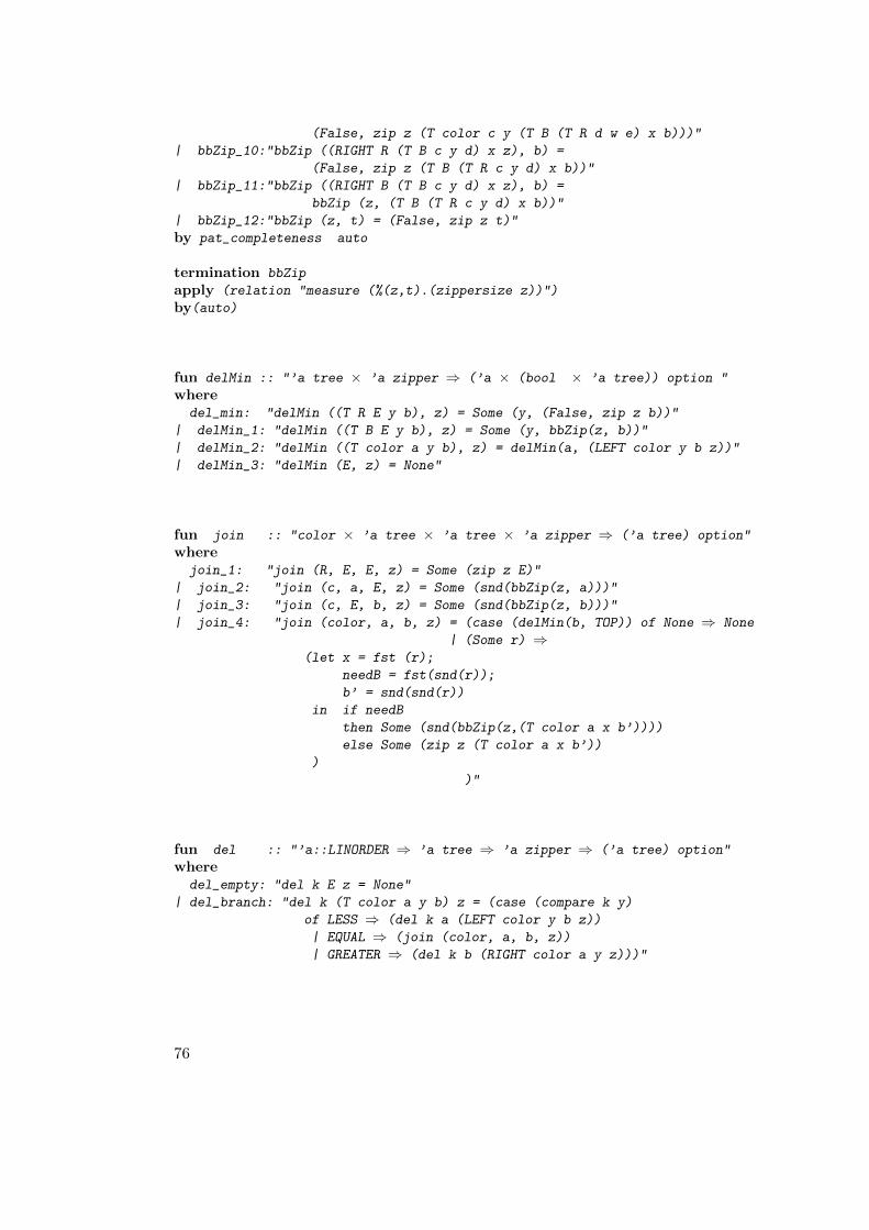
(False, zip z (T color c y (T B (T R d w e) x b)))"
| bbZip_10:"bbZip ((RIGHT R (T B c y d) x z), b) =
(False, zip z (T B (T R c y d) x b))"
| bbZip_11:"bbZip ((RIGHT B (T B c y d) x z), b) =
bbZip (z, (T B (T R c y d) x b))"
| bbZip_12:"bbZip (z, t) = (False, zip z t)"
by pat_completeness auto
termination bbZip
apply (relation "measure (%(z,t).(zippersize z))")
by(auto)
fun delMin :: "’a tree × ’a zipper ⇒ (’a × (bool × ’a tree)) option "
wheredel_min: "delMin ((T R E y b), z) = Some (y, (False, zip z b))"
| delMin_1: "delMin ((T B E y b), z) = Some (y, bbZip(z, b))"
| delMin_2: "delMin ((T color a y b), z) = delMin(a, (LEFT color y b z))"
| delMin_3: "delMin (E, z) = None"
fun join :: "color × ’a tree × ’a tree × ’a zipper ⇒ (’a tree) option"
wherejoin_1: "join (R, E, E, z) = Some (zip z E)"
| join_2: "join (c, a, E, z) = Some (snd(bbZip(z, a)))"
| join_3: "join (c, E, b, z) = Some (snd(bbZip(z, b)))"
| join_4: "join (color, a, b, z) = (case (delMin(b, TOP)) of None ⇒ None
| (Some r) ⇒(let x = fst (r);
needB = fst(snd(r));
b’ = snd(snd(r))
in if needB
then Some (snd(bbZip(z,(T color a x b’))))
else Some (zip z (T color a x b’))
)
)"
fun del :: "’a::LINORDER ⇒ ’a tree ⇒ ’a zipper ⇒ (’a tree) option"
wheredel_empty: "del k E z = None"
| del_branch: "del k (T color a y b) z = (case (compare k y)
of LESS ⇒ (del k a (LEFT color y b z))
| EQUAL ⇒ (join (color, a, b, z))
| GREATER ⇒ (del k b (RIGHT color a y z)))"
76
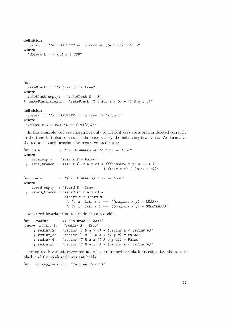
definitiondelete :: "’a::LINORDER ⇒ ’a tree ⇒ (’a tree) option"
where"delete k t ≡ del k t TOP"
funmakeBlack :: "’a tree ⇒ ’a tree"
wheremakeBlack_empty: "makeBlack E = E"
| makeBlack_branch: "makeBlack (T color a x b) = (T B a x b)"
definitioninsert :: "’a::LINORDER ⇒ ’a tree ⇒ ’a tree"
where"insert x t ≡ makeBlack (ins(x,t))"
In this example we have chosen not only to check if keys are stored or deleted correctlyin the trees but also to check if the trees satisfy the balancing invariants. We formalizethe red and black invariant by recursive predicates:
fun isin :: "’a::LINORDER ⇒ ’a tree ⇒ bool"
whereisin_empty : "isin x E = False"
| isin_branch : "isin x (T c a y b) = (((compare x y) = EQUAL)
| (isin x a) | (isin x b))"
fun isord :: "(’a::LINORDER) tree ⇒ bool"
whereisord_empty : "isord E = True"
| isord_branch : "isord (T c a y b) =
(isord a ∧ isord b
∧ (∀ x. isin x a −→ ((compare x y) = LESS))
∧ (∀ x. isin x b −→ ((compare x y) = GREATER)))"
weak red invariant: no red node has a red child
fun redinv :: "’a tree ⇒ bool"
where redinv_1: "redinv E = True"
| redinv_2: "redinv (T B a y b) = (redinv a ∧ redinv b)"
| redinv_3: "redinv (T R (T R a x b) y c) = False"
| redinv_4: "redinv (T R a x (T R b y c)) = False"
| redinv_5: "redinv (T R a x b) = (redinv a ∧ redinv b)"
strong red invariant: every red node has an immediate black ancestor, i.e. the root isblack and the weak red invariant holds
fun strong_redinv :: "’a tree ⇒ bool"
77
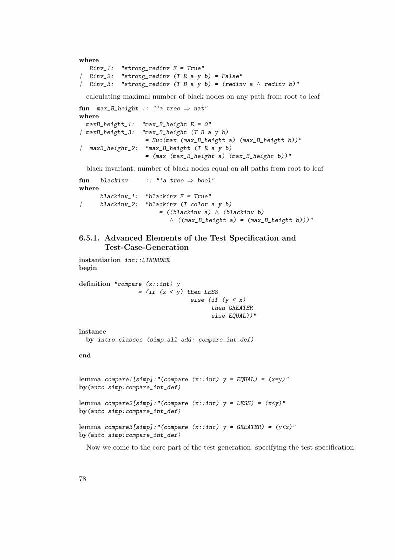
whereRinv_1: "strong_redinv E = True"
| Rinv_2: "strong_redinv (T R a y b) = False"
| Rinv_3: "strong_redinv (T B a y b) = (redinv a ∧ redinv b)"
calculating maximal number of black nodes on any path from root to leaf
fun max_B_height :: "’a tree ⇒ nat"
wheremaxB_height_1: "max_B_height E = 0"
| maxB_height_3: "max_B_height (T B a y b)
= Suc(max (max_B_height a) (max_B_height b))"
| maxB_height_2: "max_B_height (T R a y b)
= (max (max_B_height a) (max_B_height b))"
black invariant: number of black nodes equal on all paths from root to leaf
fun blackinv :: "’a tree ⇒ bool"
whereblackinv_1: "blackinv E = True"
| blackinv_2: "blackinv (T color a y b)
= ((blackinv a) ∧ (blackinv b)
∧ ((max_B_height a) = (max_B_height b)))"
6.5.1. Advanced Elements of the Test Specification andTest-Case-Generation
instantiation int::LINORDER
begin
definition "compare (x::int) y
= (if (x < y) then LESS
else (if (y < x)
then GREATER
else EQUAL))"
instanceby intro_classes (simp_all add: compare_int_def)
end
lemma compare1[simp]:"(compare (x::int) y = EQUAL) = (x=y)"
by(auto simp:compare_int_def)
lemma compare2[simp]:"(compare (x::int) y = LESS) = (x<y)"
by(auto simp:compare_int_def)
lemma compare3[simp]:"(compare (x::int) y = GREATER) = (y<x)"
by(auto simp:compare_int_def)
Now we come to the core part of the test generation: specifying the test specification.
78
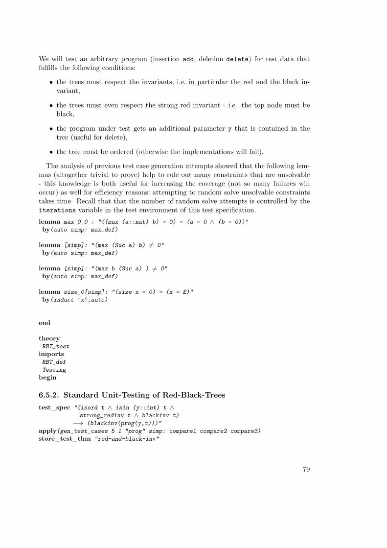
We will test an arbitrary program (insertion add, deletion delete) for test data thatfulfills the following conditions:
• the trees must respect the invariants, i.e. in particular the red and the black in-variant,
• the trees must even respect the strong red invariant - i.e. the top node must beblack,
• the program under test gets an additional parameter y that is contained in thetree (useful for delete),
• the tree must be ordered (otherwise the implementations will fail).
The analysis of previous test case generation attempts showed that the following lem-mas (altogether trivial to prove) help to rule out many constraints that are unsolvable- this knowledge is both useful for increasing the coverage (not so many failures willoccur) as well for efficiency reasons: attempting to random solve unsolvable constraintstakes time. Recall that that the number of random solve attempts is controlled by theiterations variable in the test environment of this test specification.
lemma max_0_0 : "((max (a::nat) b) = 0) = (a = 0 ∧ (b = 0))"
by(auto simp: max_def)
lemma [simp]: "(max (Suc a) b) 6= 0"
by(auto simp: max_def)
lemma [simp]: "(max b (Suc a) ) 6= 0"
by(auto simp: max_def)
lemma size_0[simp]: "(size x = 0) = (x = E)"
by(induct "x",auto)
end
theoryRBT_test
importsRBT_def
Testing
begin
6.5.2. Standard Unit-Testing of Red-Black-Trees
test spec "(isord t ∧ isin (y::int) t ∧strong_redinv t ∧ blackinv t)
−→ (blackinv(prog(y,t)))"
apply(gen_test_cases 5 1 "prog" simp: compare1 compare2 compare3)
store test thm "red-and-black-inv"
79
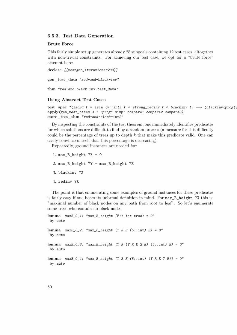
6.5.3. Test Data Generation
Brute Force
This fairly simple setup generates already 25 subgoals containing 12 test cases, altogetherwith non-trivial constraints. For achieving our test case, we opt for a “brute force”attempt here:
declare [[testgen_iterations=200]]
gen test data "red-and-black-inv"
thm "red-and-black-inv.test_data"
Using Abstract Test Cases
test spec "(isord t ∧ isin (y::int) t ∧ strong_redinv t ∧ blackinv t) −→ (blackinv(prog(y,t)))"
apply(gen_test_cases 3 1 "prog" simp: compare1 compare2 compare3)
store test thm "red-and-black-inv2"
By inspecting the constraints of the test theorem, one immediately identifies predicatesfor which solutions are difficult to find by a random process (a measure for this difficultycould be the percentage of trees up to depth k that make this predicate valid. One caneasily convince oneself that this percentage is decreasing).
Repeatedly, ground instances are needed for:
1. max_B_height ?X = 0
2. max_B_height ?Y = max_B_height ?Z
3. blackinv ?X
4. redinv ?X
The point is that enumerating some examples of ground instances for these predicatesis fairly easy if one bears its informal definition in mind. For max_B_height ?X this is:”maximal number of black nodes on any path from root to leaf”. So let’s enumeratesome trees who contain no black nodes:
lemma maxB_0_1: "max_B_height (E:: int tree) = 0"
by auto
lemma maxB_0_2: "max_B_height (T R E (5::int) E) = 0"
by auto
lemma maxB_0_3: "max_B_height (T R (T R E 2 E) (5::int) E) = 0"
by auto
lemma maxB_0_4: "max_B_height (T R E (5::int) (T R E 7 E)) = 0"
by auto
80
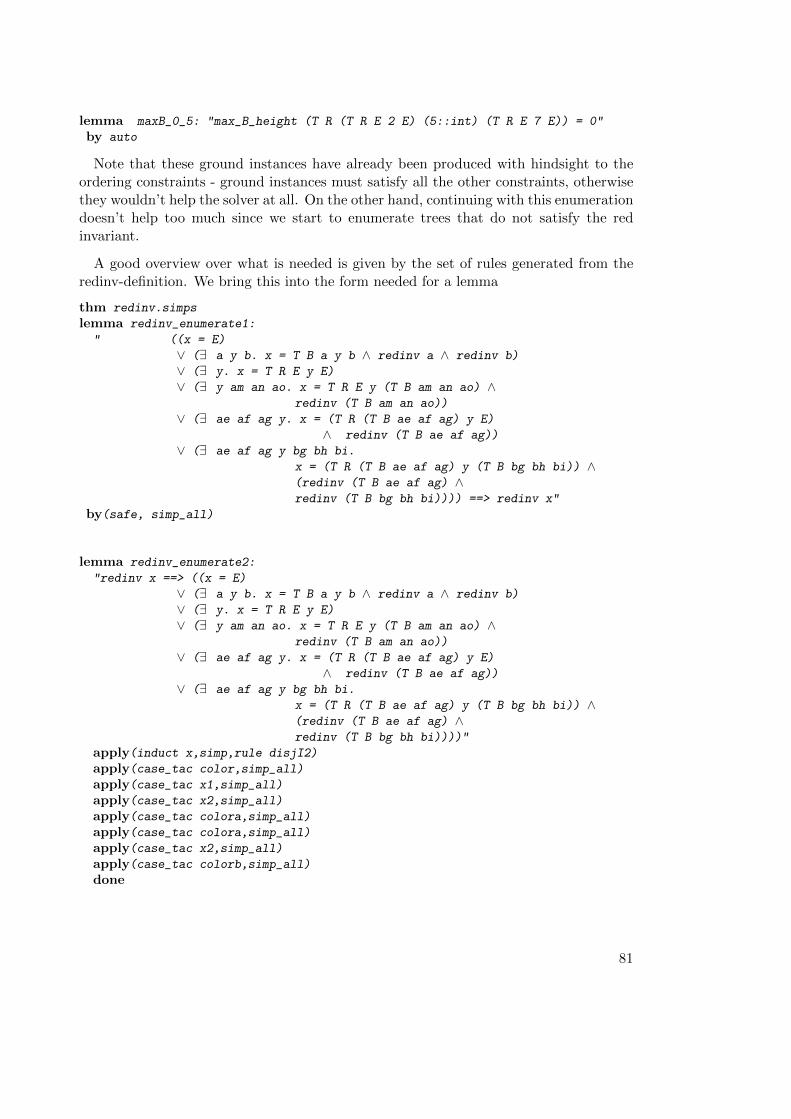
lemma maxB_0_5: "max_B_height (T R (T R E 2 E) (5::int) (T R E 7 E)) = 0"
by auto
Note that these ground instances have already been produced with hindsight to theordering constraints - ground instances must satisfy all the other constraints, otherwisethey wouldn’t help the solver at all. On the other hand, continuing with this enumerationdoesn’t help too much since we start to enumerate trees that do not satisfy the redinvariant.
A good overview over what is needed is given by the set of rules generated from theredinv-definition. We bring this into the form needed for a lemma
thm redinv.simps
lemma redinv_enumerate1:
" ((x = E)
∨ (∃ a y b. x = T B a y b ∧ redinv a ∧ redinv b)
∨ (∃ y. x = T R E y E)
∨ (∃ y am an ao. x = T R E y (T B am an ao) ∧redinv (T B am an ao))
∨ (∃ ae af ag y. x = (T R (T B ae af ag) y E)
∧ redinv (T B ae af ag))
∨ (∃ ae af ag y bg bh bi.
x = (T R (T B ae af ag) y (T B bg bh bi)) ∧(redinv (T B ae af ag) ∧redinv (T B bg bh bi)))) ==> redinv x"
by(safe, simp_all)
lemma redinv_enumerate2:
"redinv x ==> ((x = E)
∨ (∃ a y b. x = T B a y b ∧ redinv a ∧ redinv b)
∨ (∃ y. x = T R E y E)
∨ (∃ y am an ao. x = T R E y (T B am an ao) ∧redinv (T B am an ao))
∨ (∃ ae af ag y. x = (T R (T B ae af ag) y E)
∧ redinv (T B ae af ag))
∨ (∃ ae af ag y bg bh bi.
x = (T R (T B ae af ag) y (T B bg bh bi)) ∧(redinv (T B ae af ag) ∧redinv (T B bg bh bi))))"
apply(induct x,simp,rule disjI2)
apply(case_tac color,simp_all)
apply(case_tac x1,simp_all)
apply(case_tac x2,simp_all)
apply(case_tac colora,simp_all)
apply(case_tac colora,simp_all)
apply(case_tac x2,simp_all)
apply(case_tac colorb,simp_all)
done
81
lemma redinv_enumerate:
"redinv x =((x = E)
∨ (∃ a y b. x = T B a y b ∧ redinv a ∧ redinv b)
∨ (∃ y. x = T R E y E)
∨ (∃ y am an ao. x = T R E y (T B am an ao) ∧redinv (T B am an ao))
∨ (∃ ae af ag y. x = (T R (T B ae af ag) y E)
∧ redinv (T B ae af ag))
∨ (∃ ae af ag y bg bh bi.
x = (T R (T B ae af ag) y (T B bg bh bi)) ∧(redinv (T B ae af ag) ∧redinv (T B bg bh bi))))"
apply(rule iffI)
apply(rule redinv_enumerate2, assumption)
apply(rule redinv_enumerate1, assumption)
done
An Alternative Approach with a little Theorem Proving
This approach will suffice to generate the critical test data revealing the error in thesml/NJ library.
Alternatively, one might:
1. use abstract test cases for the auxiliary predicates redinv and blackinv,
2. increase the depth of the test case generation and introduce auxiliary lemmas, thatallow for the elimination of unsatisfiable constraints,
3. or applying more brute force.
Of course, one might also apply a combination of these techniques in order to get amore systematic test than the one presented here.
We will describe option 2 briefly in more detail: part of the following lemmas requireinduction and real theorem proving, but help to refine constraints systematically.
lemma height_0:
"(max_B_height x = 0) =
(x = E ∨ (∃ a y b. x = T R a y b ∧(max (max_B_height a) (max_B_height b)) = 0))"
by(induct "x", simp_all,case_tac "color",auto)
lemma max_B_height_dec: "((max_B_height (T x t1 val t3)) = 0) =⇒ (x = R) "
by(case_tac "x",auto)
This paves the way for the following testing scenario, which separates the test gen-eration phase from the introduction of the uniformity hypothesis (and, thus, the intro-
82
duction of proof obligations). This way, we can manipulate the test theorem before”freezing” it into the standard format amenable for the test data generation phase.
test spec "(isord t ∧ isin (y::int) t ∧strong_redinv t ∧ blackinv t)
−→ (blackinv(prog(y,t)))"
... introduces locally into the proof-state an option of gen_test_cases that omits constranitgeneration.
using[[testgen_no_finalize]]apply(gen_test_cases 3 1 "prog" simp: compare1 compare2 compare3
max_B_height_dec)
... intermediate steps ...
apply(simp_all only: height_0, simp_all add: max_0_0)
apply(simp_all only: height_0, simp_all add: max_0_0)
apply(safe,simp_all)
brings the test theorem back into the standard format. :
apply(tactic "TestGen.finalize_tac @{context} ["prog"]")
store test thm "red-and-black-inv3"
declare [[testgen_iterations=20]]
gen test data "red-and-black-inv3"
thm "red-and-black-inv3.test_data"
The inspection shows now a stream-lined, quite powerful test data set for our problem.Note that the ”depth 3” parameter of the test case generation leads to ”depth 2” trees,since the constructor E is counted. Nevertheless, this test case produces the error regu-larly (Warning: recall that randomization is involved; in general, this makes the searchfaster (while requiring less control by the user) than brute force enumeration, but hasthe prize that in rare cases the random solver does not find the solution at all):
blackinv (prog (1, T B E 1 E))
blackinv (prog (-7, T B E -7 (T R E 2 E)))
blackinv (prog (2, T B E -8 (T R E 2 E)))
blackinv (prog (-1, T B (T R E -7 E) -1 E))
blackinv (prog (-3, T B (T R E -3 E) -1 E))
blackinv (prog (1, T B (T R E -7 E) 1 (T R E 9 E)))
blackinv (prog (-4, T B (T B E -4 E) 3 (T B E 6 E)))
blackinv (prog (-7, T B (T R E -10 E) -9 (T R E -7 E)))
When increasing the depth to 5, the test case generation is still feasible - we had runswhich took less than two minutes and resulted in 348 test cases.
83
6.5.4. Configuring the Code Generator
We have to perform the usual setup of the internal Isabelle code generator, which involvesproviding suitable ground instances of generic functions (in current Isabelle) and the mapof the data structures to the data structures in the environment.
Note that in this setup the mapping to the target program under test is done in thewrapper script, that also maps our abstract trees to more concrete data structures asused in the implementation.
declare [[testgen_setup_code="open IntRedBlackSet;",
testgen_toString="wrapper.toString"]]
types codecolor ("color")
ml_order ("order")
tree ("_ tree")
consts code"compare" ("Key.compare (_,_)")
"color.B" ("B")
"color.R" ("R")
"tree.E" ("E")
"tree.T" ("(T(_,_,_,_))")
Now we can generate a test script (for both test data sets):
gen test script "rbt_script.sml" "red-and-black-inv" "prog"
"wrapper.del"
gen test script "rbt2_script.sml" "red-and-black-inv3" "prog"
"wrapper.del"
6.5.5. Test Result Verification
Running the test executable (either based on red-and-black-inv or on red-and-black-inv3)results in an output similar to
Test Results:
=============
Test 0 - SUCCESS, result: E
Test 1 - SUCCESS, result: T(R,E,67,E)
Test 2 - SUCCESS, result: T(B,E,~88,E)
Test 3 - ** WARNING: pre-condition false (exception
during post_condition)
Test 4 - ** WARNING: pre-condition false (exception
during post_condition)
84
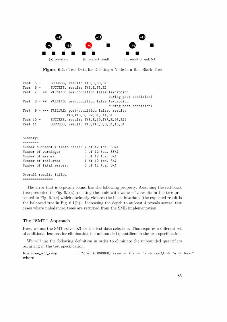
−11
−42
−92
(a) pre-state
−92
−11
(b) correct result
−92
−11
(c) result of sml/NJ
Figure 6.1.: Test Data for Deleting a Node in a Red-Black Tree
Test 5 - SUCCESS, result: T(R,E,30,E)
Test 6 - SUCCESS, result: T(B,E,73,E)
Test 7 - ** WARNING: pre-condition false (exception
during post_condition)
Test 8 - ** WARNING: pre-condition false (exception
during post_condition)
Test 9 - *** FAILURE: post-condition false, result:
T(B,T(B,E,~92,E),~11,E)
Test 10 - SUCCESS, result: T(B,E,19,T(R,E,98,E))
Test 11 - SUCCESS, result: T(B,T(R,E,8,E),16,E)
Summary:
--------
Number successful tests cases: 7 of 12 (ca. 58%)
Number of warnings: 4 of 12 (ca. 33%)
Number of errors: 0 of 12 (ca. 0%)
Number of failures: 1 of 12 (ca. 8%)
Number of fatal errors: 0 of 12 (ca. 0%)
Overall result: failed
===============
The error that is typically found has the following property: Assuming the red-blacktree presented in Fig. 6.1(a), deleting the node with value −42 results in the tree pre-sented in Fig. 6.1(c) which obviously violates the black invariant (the expected result isthe balanced tree in Fig. 6.1(b)). Increasing the depth to at least 4 reveals several testcases where unbalanced trees are returned from the SML implementation.
The ”SMT” Approach
Here, we use the SMT solver Z3 for the test data selection. This requires a different setof additional lemmas for eliminating the unbounded quantifiers in the test specification.
We will use the following definition in order to eliminate the unbounded quantifiersoccurring in the test specification.
fun tree_all_comp :: "(’a::LINORDER) tree ⇒ (’a ⇒ ’a ⇒ bool) ⇒ ’a ⇒ bool"
where
85
tree_all_comp_empty : "tree_all_comp E c y = True"
| tree_all_comp_branch : "tree_all_comp (T rb a x b) c y = ((c x y) ∧ (tree_all_comp
a c y) ∧ (tree_all_comp b c y))"
The following lemma states how the unbounded quantifier in the test specification canbe expressed using the function tree_all_comp.
lemma all_eq: "(tree_all_comp a c y) = (∀ x. isin x a −→ c x y)"
apply(auto)apply(erule rev_mp)+
apply(induct_tac a)
apply(auto)apply(simp add: LINORDER_equal)
apply(erule rev_mp)+
apply(induct_tac a)
apply(auto)apply(simp add: LINORDER_equal)
done
In order to avoid lambda-expressions in the test specification that may be problematicfor SMT solvers, we define the following two specific tree comparison functions.
fun tree_all_less :: "(’a::LINORDER) tree ⇒ ’a ⇒ bool"
wheretree_all_less_d: "tree_all_less a y = (tree_all_comp a (λu v .(compare u v) =
LESS)) y"
fun tree_all_greater :: "(’a::LINORDER) tree ⇒ ’a ⇒ bool"
wheretree_all_greater_d: "tree_all_greater a y = (tree_all_comp a (λu v.(compare u
v) = GREATER)) y"
Using these new functions, we are able to provide a new definition of isord that doesnot rely on an unbounded quantifier.
fun isord’ :: "(’a::LINORDER) tree ⇒ bool"
whereisord_empty’ : "isord’ E = True"
| isord_branch’ : "isord’ (T c a y b) =
(isord’ a ∧ isord’ b
∧ (tree_all_less a y)
∧ (tree_all_greater b y))"
lemma isord_subst: "isord t = isord’ t"
apply(induct_tac t)
apply(auto)apply(simp_all add: all_eq)
done
We now instantiate the recursive definition of tree_all_comp in order to obtain re-cursive definitions for tree_all_less and tree_all_greater.
86
declare tree_all_less_d [simp del]
declare tree_all_greater_d [simp del]
lemmas tree_all_less_inv [simp] = tree_all_less_d[THEN sym]
lemmas tree_all_greater_inv [simp] = tree_all_greater_d[THEN sym]
declare tree_all_comp_branch [simp del]
lemmas tree_all_less_empty [simp] = tree_all_comp_empty[where c = "(λx y.(compare
x y) = LESS)",simplified]
lemmas tree_all_less_branch [simp] = tree_all_comp_branch [where c = "(λx y.(compare
x y) = LESS)", simplified]
lemmas tree_all_greater_empty [simp] = tree_all_comp_empty[where c = "(λx y.(compare
x y) = GREATER)", simplified]
lemmas tree_all_greater_branch [simp] = tree_all_comp_branch [where c = "(λx y.(compare
x y) = GREATER)", simplified]
declare isord_branch’ [simp del]
lemmas isord_branch’’ [simp] = isord_branch’[simplified]
declare [[testgen_no_finalize=false]]
test spec "(isord t ∧ isin (y::int) t ∧strong_redinv t ∧ blackinv t)
−→ prog(y,t)"
apply(simp add: isord_subst)
apply(gen_test_cases 5 1 "prog" simp: compare1 compare2 compare3)
store test thm "red-and-black-inv-smt"
6.5.6. Test Data Generation
declare [[testgen_SMT]]
declare [[testgen_iterations=0]]
declare [[ smt_solver = z3 ]]
declare [[ z3_options = "AUTO_CONFIG=false MBQI=false" ]]
declare [[smt_datatypes=true]]
declare [[smt_timeout = 300]]
declare [[smt_oracle = true]]
declare tree.size(3) [testgen_smt_facts]
declare tree.size(4) [testgen_smt_facts]
declare color.size(3) [testgen_smt_facts]
declare color.size(4) [testgen_smt_facts]
declare isord_empty’ [testgen_smt_facts]
declare isord_branch’’ [testgen_smt_facts]
declare tree_all_less_empty [testgen_smt_facts]
declare tree_all_less_branch [testgen_smt_facts]
87
declare tree_all_greater_empty [testgen_smt_facts]
declare tree_all_greater_branch [testgen_smt_facts]
declare isin.simps [testgen_smt_facts]
declare compare_int_def [testgen_smt_facts]
declare blackinv.simps [testgen_smt_facts]
declare max_B_height.simps [testgen_smt_facts]
declare strong_redinv.simps [testgen_smt_facts]
declare redinv.simps [testgen_smt_facts]
gen test data "red-and-black-inv-smt"
thm "red-and-black-inv-smt.test_data"
end
6.6. Sequence Testing
In this section, we apply HOL-TestGen to different sequence testing scenarios; see [13]for more details.
6.6.1. Reactive Sequence Testing
theory Sequence_test
importsList
Testing
begin
This notation consideres failures as valid – a definition inspired by I/O conformance...
In this theory, we present a simple reactive system and demonstrate and show howHOL-TestGencan be used for testing such systems.
Our scenario is motivated by the following communcation scenario: A client sendsa communication request to a server and specifies a port-range X. The server non-deterministically chooses a port Y which is within the specified range. The client sendsa sequence of data (abstracted away in our example to a constant Data) on the portallocated by the server. The communication is terminated by the client with a stop
event. Using a csp-like notation, we can describe such a system as follows: req?X →port?Y [Y < X] → (rec N • send !D,Y → ack → N � stop → ack → SKIP) It isnecessary for our approach that the protocol strictly alternates client-side and server-side events; thus, we will be able to construct in a test of the server a step-function ioprog(see below) that stimulates the server with an input and records its result. If a protocoldoes not have alternation in its events, it must be constructed by artificial acknowledgeevents; it is then a question of their generation in the test harness if they were sentanyway or if they correspond to something like “server reacted within timebounds.”
88
The stimulation sequence of the system under test results just from the projection ofthis protocol to the input events: req?X → (rec N • send !D,Y → N � stop → SKIP)
6.6.2. Basic Technique: Events with explicit variables
We define abstract traces containing explicit variables X, Y , . . . . The whole test casegeneration is done on the basis of the abstract traces. However, some small additionalfunctions substitute and bind were used to replace them with concrete values during therun of the test-driver, as well as programs that check pre and post conditions on theconcrete values occuring in the concrete run.
We specify explicit variables and a joined type containing abstract events (replacingvalues by explicit variables) as well as their concrete counterparts.
datatype vars = X | Y
datatype data = Data
types chan = int
datatype InEvent_conc = req chan | send data chan | stop
datatype InEvent_abs = reqA vars | sendA data vars | stopA
datatype OutEvent_conc = port chan | ack
datatype OutEvent_abs = portA vars | ackA
constdefs lookup :: "[’a ⇀ ’b, ’a] ⇒ ’b"
"lookup env v ≡ the(env v)"
success:: "’α option ⇒ bool"
"success x ≡ case x of None => False | Some x => True"
types InEvent = "InEvent_abs + InEvent_conc"
types OutEvent = "OutEvent_abs + OutEvent_conc"
types event_abs = "InEvent_abs + OutEvent_abs"
setup{*map_testgen_params(TestGen.breadth_update 15)*}
ML{*TestGen_DataManagement.get(Context.Theory(the_context()))*}
ML{*val prms = goal (theory "Main") "H = G";*}
ML{* concl_of(topthm()) *}
6.6.3. The infrastructure of the observer: substitute and rebind
The predicate substitute allows for mapping abstract events containing explicit vari-ables to concrete events by substituting the variables by values communicated in thesystem run. It requires an environment (“substitution”) where the concrete values oc-curing in the system run were assigned to variables.
89
consts substitute :: "[vars ⇀ chan, InEvent_abs] ⇒ InEvent_conc"
primrec"substitute env (reqA v) = req(lookup env v)"
"substitute env (sendA d v)= send d (lookup env v)"
"substitute env stopA = InEvent_conc.stop"
The predicate rebind extracts from concrete output events the values and binds themto explicit variables in env. It should never be applied to abract values; therefore, wewe can use an underspecified version (arbitrary). The predicate rebind only stores ?-occurrences in the protocol into the environment; !-occurences are ignored. Events thatare the same in the abstract as well as the concrete setting are treated as abstract events.
In a way, rebind can be viewed as an abstraction of the concrete log produced atruntime.
consts rebind :: "[vars ⇀ chan, OutEvent_conc] ⇒ vars ⇀ chan"
primrec"rebind env (port n) = env(Y 7→ n)"
"rebind env OutEvent_conc.ack = env"
6.6.4. Abstract Protocols and Abstract Stimulation Sequences
Now we encode the protocol automaton (abstract version) by a recursive acceptancepredicate. One could project the set of stimulation sequences just by filtering out theoutEvents occuring in the traces.
We will not pursue this approach since a more constructive presentation of the stim-ulation sequence set is advisable for testing.
However, we show here how such concepts can be specified.
syntax A :: "nat" B :: "nat" C :: "nat"
D :: "nat" E :: "nat"
translations"A" == "0" "B" == "Suc A" "C" == "Suc B"
"D" == "Suc C" "E" == "Suc D"
consts accept’ :: "nat × event_abs list ⇒ bool"
recdef accept’ "measure(λ (x,y). length y)"
"accept’(A,(Inl(reqA X))#S) = accept’(B,S)"
"accept’(B,(Inr(portA Y))#S) = accept’(C,S)"
"accept’(C,(Inl(sendA d Y))#S) = accept’(D,S)"
"accept’(D,(Inr(ackA))#S) = accept’(C,S)"
"accept’(C,(Inl(stopA))#S) = accept’(E,S)"
"accept’(E,[Inr(ackA)]) = True"
"accept’(x,y) = False"
constdefsaccept :: "event_abs list ⇒ bool"
"accept s ≡ accept’(0,s)"
We proceed by modeling a subautomaton of the protocol automaton accept.
90
consts stim_trace’ :: "nat × InEvent_abs list ⇒ bool"
recdef stim_trace’ "measure(λ (x,y). length y)"
"stim_trace’(A,(reqA X)#S) = stim_trace’(C,S)"
"stim_trace’(C,(sendA d Y)#S) = stim_trace’(C,S)"
"stim_trace’(C,[stopA]) = True"
"stim_trace’(x,y) = False"
constdefs stim_trace :: "InEvent_abs list ⇒ bool"
"stim_trace s ≡ stim_trace’(A,s)"
6.6.5. The Post-Condition
consts postcond’ :: "((vars ⇀ int) × ’σ × InEvent_conc × OutEvent_conc) ⇒ bool"
recdef postcond’ "{}"
"postcond’ (env, x, req n, port m) = (m <= n)"
"postcond’ (env, x, send z n, OutEvent_conc.ack) = (n = lookup env Y)"
"postcond’ (env, x, InEvent_conc.stop, OutEvent_conc.ack) = True"
"postcond’ (env, x, y, z) = False"
constdefs postcond :: "(vars ⇀ int) ⇒ ’σ ⇒ InEvent_conc ⇒ OutEvent_conc ⇒ bool"
"postcond env σ y z ≡ postcond’ (env, σ, y, z)"
6.6.6. Testing for successful system runs of the server under test
So far, we have not made any assumption on the state σ′ of the program under testioprog. It could be a log of the actual system run. However, for simplicity, we use onlya trivial state in this test specification.
6.6.7. Test-Generation: The Standard Approach
declare stim_trace_def[simp]
test spec "stim_trace trace −→((empty(X7→init_value),()) |= (os ← (mbind trace ioprog) ; result(length
trace = length os)))"
apply(gen_test_cases 4 1 "ioprog" )
store test thm "reactive"
testgen params [iterations=1000]
91
6.6.8. Test-Generation: Refined Approach involving TP
An analysis of the previous approach shows that random solving on trace patterns isobviously still quite ineffective. Although path coverage wrt. the input stimulationtrace automaton can be achieved with a reasonable high probability, the depth remainslimited.
The idea is to produce a better test theorem by more specialized rules, that take thespecial form of the input stimulation protocol into account.
lemma start :
"stim_trace’(A,x#S) = ((x = reqA X) ∧ stim_trace’(C,S))"
apply(cases "x", simp_all)
apply(rule_tac y="vars" in vars.exhaust,simp_all)
done
lemma final[simp]:
"(stim_trace’ (x, stopA # S)) = ((x=C)∧(S=[]))"apply(case_tac "x=Suc (Suc (A::nat))", simp_all)
apply(cases "S",simp_all)
apply(case_tac "x=Suc (A::nat)", simp_all)
apply(case_tac "x = (A::nat)", simp_all)
apply(subgoal_tac "∃ xa. x = Suc(Suc(Suc xa))",erule exE,simp)
apply(arith)done
lemma step1 :
"stim_trace’(C,x#y#S) = ((x=sendA Data Y) ∧ stim_trace’(C,y#S))"
apply(cases "x", simp_all)
apply(rule_tac y="data" in data.exhaust,simp_all)
apply(rule_tac y="vars" in vars.exhaust,simp_all)
done
lemma step2:
"stim_trace’(C,[x]) = (x=stopA)"
apply(cases "x", simp_all)
apply(rule_tac y="data" in data.exhaust,simp_all)
apply(rule_tac y="vars" in vars.exhaust,simp_all)
done
The three rules start, step1 and step2 give us a translation of a constraint of the formstim trace′(x, [a, . . . , b]) into a simple conjunction of equalities (in general: disjunctionand existential quantifier will also occur). Since a formula of this form is an easy game forfast tac inside gen test cases, we will get dramatically better test theorems, wherethe constraints have been resolved already.
We reconfigure the rewriter:
declare start[simp] step1[simp] step2 [simp]
test spec "stim_trace ιs −→
92
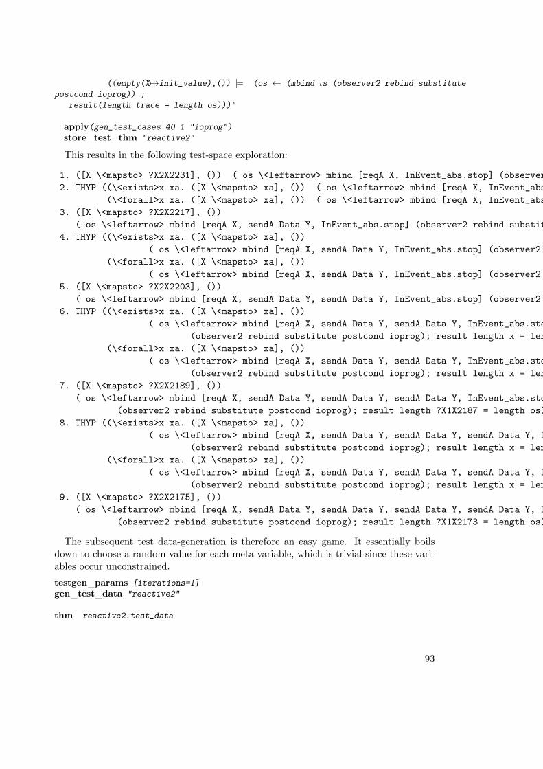
((empty(X7→init_value),()) |= (os ← (mbind ιs (observer2 rebind substitute
postcond ioprog)) ;
result(length trace = length os)))"
apply(gen_test_cases 40 1 "ioprog")
store test thm "reactive2"
This results in the following test-space exploration:
1. ([X \<mapsto> ?X2X2231], ()) ( os \<leftarrow> mbind [reqA X, InEvent_abs.stop] (observer2 rebind substitute postcond ioprog); result length ?X1X2229 = length os)
2. THYP ((\<exists>x xa. ([X \<mapsto> xa], ()) ( os \<leftarrow> mbind [reqA X, InEvent_abs.stop] (observer2 rebind substitute postcond ioprog); result length x = length os)) \<longrightarrow>
(\<forall>x xa. ([X \<mapsto> xa], ()) ( os \<leftarrow> mbind [reqA X, InEvent_abs.stop] (observer2 rebind substitute postcond ioprog); result length x = length os)))
3. ([X \<mapsto> ?X2X2217], ())
( os \<leftarrow> mbind [reqA X, sendA Data Y, InEvent_abs.stop] (observer2 rebind substitute postcond ioprog); result length ?X1X2215 = length os)
4. THYP ((\<exists>x xa. ([X \<mapsto> xa], ())
( os \<leftarrow> mbind [reqA X, sendA Data Y, InEvent_abs.stop] (observer2 rebind substitute postcond ioprog); result length x = length os)) \<longrightarrow>
(\<forall>x xa. ([X \<mapsto> xa], ())
( os \<leftarrow> mbind [reqA X, sendA Data Y, InEvent_abs.stop] (observer2 rebind substitute postcond ioprog); result length x = length os)))
5. ([X \<mapsto> ?X2X2203], ())
( os \<leftarrow> mbind [reqA X, sendA Data Y, sendA Data Y, InEvent_abs.stop] (observer2 rebind substitute postcond ioprog); result length ?X1X2201 = length os)
6. THYP ((\<exists>x xa. ([X \<mapsto> xa], ())
( os \<leftarrow> mbind [reqA X, sendA Data Y, sendA Data Y, InEvent_abs.stop]
(observer2 rebind substitute postcond ioprog); result length x = length os)) \<longrightarrow>
(\<forall>x xa. ([X \<mapsto> xa], ())
( os \<leftarrow> mbind [reqA X, sendA Data Y, sendA Data Y, InEvent_abs.stop]
(observer2 rebind substitute postcond ioprog); result length x = length os)))
7. ([X \<mapsto> ?X2X2189], ())
( os \<leftarrow> mbind [reqA X, sendA Data Y, sendA Data Y, sendA Data Y, InEvent_abs.stop]
(observer2 rebind substitute postcond ioprog); result length ?X1X2187 = length os)
8. THYP ((\<exists>x xa. ([X \<mapsto> xa], ())
( os \<leftarrow> mbind [reqA X, sendA Data Y, sendA Data Y, sendA Data Y, InEvent_abs.stop]
(observer2 rebind substitute postcond ioprog); result length x = length os)) \<longrightarrow>
(\<forall>x xa. ([X \<mapsto> xa], ())
( os \<leftarrow> mbind [reqA X, sendA Data Y, sendA Data Y, sendA Data Y, InEvent_abs.stop]
(observer2 rebind substitute postcond ioprog); result length x = length os)))
9. ([X \<mapsto> ?X2X2175], ())
( os \<leftarrow> mbind [reqA X, sendA Data Y, sendA Data Y, sendA Data Y, sendA Data Y, InEvent_abs.stop]
(observer2 rebind substitute postcond ioprog); result length ?X1X2173 = length os)
The subsequent test data-generation is therefore an easy game. It essentially boilsdown to choose a random value for each meta-variable, which is trivial since these vari-ables occur unconstrained.
testgen params [iterations=1]
gen test data "reactive2"
thm reactive2.test_data
93
Within the timeframe of 1 minute, we get trace lengths of about 40 in the stimulationinput protocol, which corresponds to traces of 80 in the standard protocol. The examplesshows, that it is not the length of traces that is a limiting factor of our approach. Themain problem is the complexity in the stimulation automaton (size, branching-factors,possible instantiations of parameter input).
end
6.6.9. Deterministic Bank Example
theoryBank
importsTesting
begin
declare [[testgen_profiling]]
The intent of this little example is to model deposit, check and withdraw operations of alittle Bank model in pre-postcondition style, formalize them in a setup for HOL-TestGentest sequence generation and to generate elementary test cases for it. The test scenarioswill be restricted to strict sequence checking; this excludes aspects of account creationwhich will give the entire model a protocol character (a create-operation would createan account number, and then all later operations are just refering to this number; thusthere would be a dependence between system output and input as in reactive sequencetest scenarios.).
Moreover, in this scenario, we assume that the system under test is deterministic.
The state of our bank is just modeled by a map from client/account information tothe balance.
type synonym client = string
type synonym account_no = int
type synonym register = "(client × account_no) ⇀ int"
Operation definitions A standard, JML or OCL or VCC like interface specificationmight look like:
op deposit (c : client, no : account_no, amount:nat) : unit
pre (c,no) : dom(register)
post register’=register[(c,no) := register(c,no) + amount]
op balance (c : client, no : account_no) : int
94
pre (c,no) : dom(register)
post register’=register and result = register(c,no)
op withdraw(c : client, no : account_no, amount:nat) : unit
pre (c,no) : dom(register) and register(c,no) >= amount
post register’=register[(c,no) := register(c,no) - amount]
Interface normalization turns this interface into the following input type:
datatype in_c = deposit client account_no nat
| withdraw client account_no nat
| balance client account_no
datatype out_c = depositO| balanceO nat | withdrawO
fun precond :: "register ⇒ in_c ⇒ bool"
where "precond σ (deposit c no m) = ((c,no) ∈ dom σ)"| "precond σ (balance c no) = ((c,no) ∈ dom σ)"| "precond σ (withdraw c no m) = ((c,no) ∈ dom σ ∧ (int m) ≤ the(σ(c,no)))"
fun postcond :: "in_c ⇒ register ⇒ out_c × register ⇒ bool"
where "postcond (deposit c no m) σ =
(λ (n,σ’). (n = depositO ∧ σ’=σ((c,no)7→ the(σ(c,no)) + int m)))"
| "postcond (balance c no) σ =
(λ (n,σ’). (σ=σ’ ∧ (∃ x. balanceO x = n ∧ x = nat(the(σ(c,no))))))"| "postcond (withdraw c no m) σ =
(λ (n,σ’). (n = withdrawO ∧ σ’=σ((c,no)7→ the(σ(c,no)) - int m)))"
Proving Symbolic Execution Rules for the Abstractly Constructed ProgramUsing the Operators impl and strong_impl, we can synthesize an abstract programright away from the specification, i.e. the pair of pre- and postcondition defined above.Since this program is even deterministic, we derive a set of symbolic execution rules usedin the test case generation process which will produce symbolic results against which thePUT can be compared in the test driver.
lemma precond_postcond_implementable:
"implementable precond postcond"
apply(auto simp: implementable_def)
apply(case_tac "ι", simp_all)
done
The following lemmas reveal that this ”constructed” program is actually (due to de-terminism of the spec):
lemma impl_1:
"strong_impl precond postcond (deposit c no m) =
(λσ . if (c, no) ∈ dom σthen Some(depositO,σ((c, no) 7→ the (σ (c, no)) + int m))
95
else None)"
by(rule ext, auto simp: strong_impl_def )
lemma valid_both_spec1[simp]:
"(σ |= (s ← mbind ((deposit c no m)#S) (strong_impl precond postcond);
return (P s))) =
(if (c, no) ∈ dom σthen (σ((c, no) 7→ the (σ (c, no)) + int m) )|= (s ← mbind S (strong_impl precond
postcond);
return (P (depositO#s)))
else (σ |= (return (P []))))"
by(auto simp: valid_both impl_1)
lemma impl_2:
"strong_impl precond postcond (balance c no) =
(λσ. if (c, no) ∈ dom σthen Some(balanceO(nat(the (σ (c, no)))),σ)else None)"
by(rule ext, auto simp: strong_impl_def Eps_split)
lemma valid_both_spec2 [simp]:
"(σ |= (s ← mbind ((balance c no)#S) (strong_impl precond postcond);
return (P s))) =
(if (c, no) ∈ dom σthen (σ |= (s ← mbind S (strong_impl precond postcond);
return (P (balanceO(nat(the (σ (c, no))))#s))))
else (σ |= (return (P []))))"
by(auto simp: valid_both impl_2)
lemma impl_3:
"strong_impl precond postcond (withdraw c no m) =
(λσ. if (c, no) ∈ dom σ ∧ (int m) ≤ the(σ(c,no))then Some(withdrawO,σ((c, no) 7→ the (σ (c, no)) - int m))
else None)"
by(rule ext, auto simp: strong_impl_def Eps_split)
lemma valid_both_spec3[simp]:
"(σ |= (s ← mbind ((withdraw c no m)#S) (strong_impl precond postcond);
return (P s))) =
(if (c, no) ∈ dom σ ∧ (int m) ≤ the(σ(c,no))then (σ((c, no) 7→ the (σ (c, no))-int m) )|= (s ← mbind S (strong_impl precond
postcond);
return (P (withdrawO#s)))
else (σ |= (return (P []))))"
by(auto simp: valid_both impl_3)
Here comes an interesting detail revealing the power of the approach: The generated
96

sequences still respect the preconditions imposed by the specification - in this case, wherewe are talking about a client for which a defined account exists and for which we willnever produce traces in which we withdraw more money than available on it.
Test Specifications fun test_purpose :: "[client, account_no, in_c list] ⇒ bool"
where"test_purpose c no [] = False"
| "test_purpose c no (a#R) = (case R of
[] ⇒ a = balance c no
| a’#R’ ⇒ (((∃ m. a = deposit c no m) ∨(∃ m. a = withdraw c no m)) ∧test_purpose c no R))"
lemma inst_eq : "f(x,y) = Some z =⇒ f(x,y) = Some z"
by auto
lemma inst_eq2 : "x = y =⇒ x = y"
by auto
test spec test_balance:
assumes account_defined: "(c,no) ∈ dom σ_0"
and test_purpose : "test_purpose c no S"
and symbolic_run_yields_x :
"σ_0 |= (s ← mbind S (strong_impl precond postcond);
return (s = x))"
shows " σ_0 |= (s ← mbind S PUT; return (s = x))"
apply(insert account_defined test_purpose symbolic_run_yields_x)
apply(gen_test_cases "PUT" split: HOL.split_if_asm)
store test thm "bank"
This results in a test-space exploration:
1. (\<lambda>a. Some 2) \<Turnstile>
( s \<leftarrow> mbind [balance ?X2X1233 ?X1X1231] PUT; return s = [balanceO 2])
2. THYP
((\<exists>x xa xb xc.
xb (xa, x) = Some xc \<longrightarrow>
(xb \<Turnstile>
( s \<leftarrow> mbind [balance xa x]
PUT; return s = [balanceO (nat xc)]))) \<longrightarrow>
(\<forall>x xa xb xc.
xb (xa, x) = Some xc \<longrightarrow>
(xb \<Turnstile>
( s \<leftarrow> mbind [balance xa x]
97
PUT; return s = [balanceO (nat xc)]))))
3. (\<lambda>a. Some 5) \<Turnstile>
( s \<leftarrow> mbind
[deposit ?X2X1190 ?X1X1188 ?X5X1196, balance ?X2X1190 ?X1X1188]
PUT; return s = [depositO, balanceO (nat (5 + int ?X5X1196))])
4. THYP
((\<exists>x xa xb xc xd xe.
xb (xa, x) = Some xc \<longrightarrow>
xb (xa, x) = Some xe \<longrightarrow>
(xb \<Turnstile>
( s \<leftarrow> mbind [deposit xa x xd, balance xa x]
PUT; return s =
[depositO, balanceO (nat (xe + int xd))]))) \<longrightarrow>
(\<forall>x xa xb xc xd xe.
xb (xa, x) = Some xc \<longrightarrow>
xb (xa, x) = Some xe \<longrightarrow>
(xb \<Turnstile>
( s \<leftarrow> mbind [deposit xa x xd, balance xa x]
PUT; return s =
[depositO, balanceO (nat (xe + int xd))]))))
5. THYP
((\<exists>x xa xb xc xd.
\<not> (\<exists>y. xb (xa, x) = Some y) \<longrightarrow>
xb (xa, x) = Some xd \<longrightarrow>
(xb \<Turnstile>
( s \<leftarrow> mbind [deposit xa x xc, balance xa x]
PUT; return s = []))) \<longrightarrow>
(\<forall>x xa xb xc xd.
\<not> (\<exists>y. xb (xa, x) = Some y) \<longrightarrow>
xb (xa, x) = Some xd \<longrightarrow>
(xb \<Turnstile>
( s \<leftarrow> mbind [deposit xa x xc, balance xa x]
PUT; return s = []))))
6. int ?X5X1088 \<le> 7 \<Longrightarrow>
(\<lambda>a. Some 7) \<Turnstile>
( s \<leftarrow> mbind
[withdraw ?X2X1082 ?X1X1080 ?X5X1088, balance ?X2X1082 ?X1X1080]
PUT; return s = [withdrawO, balanceO (nat (7 - int ?X5X1088))])
7. THYP
((\<exists>x xa xb xc xd xe.
xb (xa, x) = Some xc \<longrightarrow>
int xd \<le> xe \<longrightarrow>
xb (xa, x) = Some xe \<longrightarrow>
(xb \<Turnstile>
98
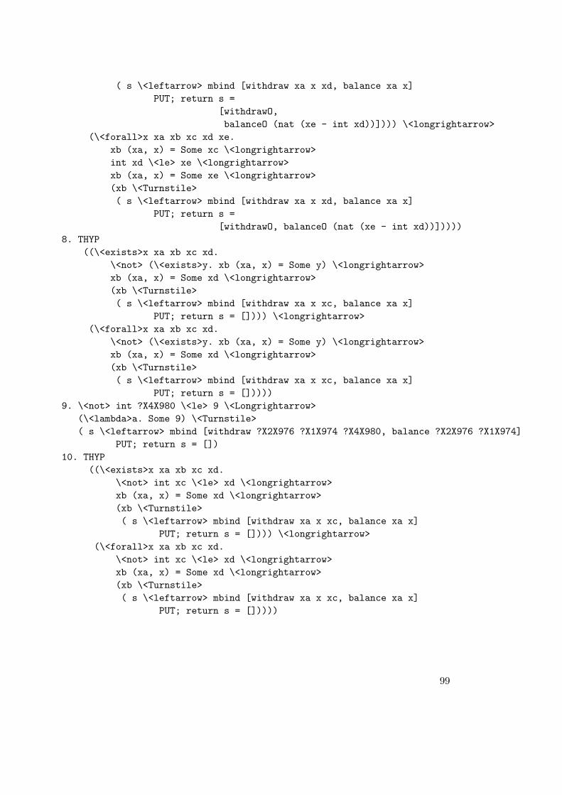
( s \<leftarrow> mbind [withdraw xa x xd, balance xa x]
PUT; return s =
[withdrawO,
balanceO (nat (xe - int xd))]))) \<longrightarrow>
(\<forall>x xa xb xc xd xe.
xb (xa, x) = Some xc \<longrightarrow>
int xd \<le> xe \<longrightarrow>
xb (xa, x) = Some xe \<longrightarrow>
(xb \<Turnstile>
( s \<leftarrow> mbind [withdraw xa x xd, balance xa x]
PUT; return s =
[withdrawO, balanceO (nat (xe - int xd))]))))
8. THYP
((\<exists>x xa xb xc xd.
\<not> (\<exists>y. xb (xa, x) = Some y) \<longrightarrow>
xb (xa, x) = Some xd \<longrightarrow>
(xb \<Turnstile>
( s \<leftarrow> mbind [withdraw xa x xc, balance xa x]
PUT; return s = []))) \<longrightarrow>
(\<forall>x xa xb xc xd.
\<not> (\<exists>y. xb (xa, x) = Some y) \<longrightarrow>
xb (xa, x) = Some xd \<longrightarrow>
(xb \<Turnstile>
( s \<leftarrow> mbind [withdraw xa x xc, balance xa x]
PUT; return s = []))))
9. \<not> int ?X4X980 \<le> 9 \<Longrightarrow>
(\<lambda>a. Some 9) \<Turnstile>
( s \<leftarrow> mbind [withdraw ?X2X976 ?X1X974 ?X4X980, balance ?X2X976 ?X1X974]
PUT; return s = [])
10. THYP
((\<exists>x xa xb xc xd.
\<not> int xc \<le> xd \<longrightarrow>
xb (xa, x) = Some xd \<longrightarrow>
(xb \<Turnstile>
( s \<leftarrow> mbind [withdraw xa x xc, balance xa x]
PUT; return s = []))) \<longrightarrow>
(\<forall>x xa xb xc xd.
\<not> int xc \<le> xd \<longrightarrow>
xb (xa, x) = Some xd \<longrightarrow>
(xb \<Turnstile>
( s \<leftarrow> mbind [withdraw xa x xc, balance xa x]
PUT; return s = []))))
99
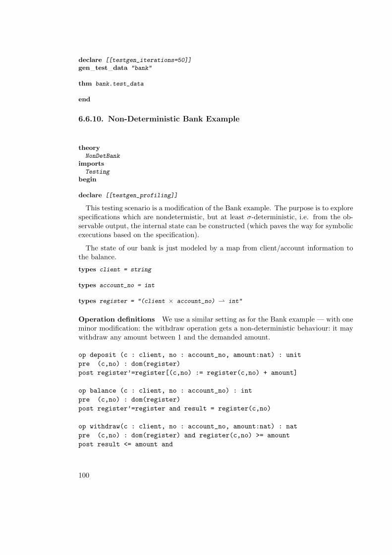
declare [[testgen_iterations=50]]
gen test data "bank"
thm bank.test_data
end
6.6.10. Non-Deterministic Bank Example
theoryNonDetBank
importsTesting
begin
declare [[testgen_profiling]]
This testing scenario is a modification of the Bank example. The purpose is to explorespecifications which are nondetermistic, but at least σ-deterministic, i.e. from the ob-servable output, the internal state can be constructed (which paves the way for symbolicexecutions based on the specification).
The state of our bank is just modeled by a map from client/account information tothe balance.
types client = string
types account_no = int
types register = "(client × account_no) ⇀ int"
Operation definitions We use a similar setting as for the Bank example — with oneminor modification: the withdraw operation gets a non-deterministic behaviour: it maywithdraw any amount between 1 and the demanded amount.
op deposit (c : client, no : account_no, amount:nat) : unit
pre (c,no) : dom(register)
post register’=register[(c,no) := register(c,no) + amount]
op balance (c : client, no : account_no) : int
pre (c,no) : dom(register)
post register’=register and result = register(c,no)
op withdraw(c : client, no : account_no, amount:nat) : nat
pre (c,no) : dom(register) and register(c,no) >= amount
post result <= amount and
100

register’=register[(c,no) := register(c,no) - result]
Interface normalization turns this interface into the following input type:
datatype in_c = deposit client account_no nat
| withdraw client account_no nat
| balance client account_no
datatype out_c = depositO| balanceO nat | withdrawO nat
fun precond :: "register ⇒ in_c ⇒ bool"
where "precond σ (deposit c no m) = ((c,no) ∈ dom σ)"| "precond σ (balance c no) = ((c,no) ∈ dom σ)"| "precond σ (withdraw c no m) = ((c,no) ∈ dom σ ∧ (int m) ≤ the(σ(c,no)))"
fun postcond :: "in_c ⇒ register ⇒ out_c × register ⇒ bool"
where "postcond (deposit c no m) σ =
(λ (n,σ’). (n = depositO ∧ σ’=σ((c,no)7→ the(σ(c,no)) + int m)))"
| "postcond (balance c no) σ =
(λ (n,σ’). (σ=σ’ ∧ (∃ x. balanceO x = n ∧ x = nat(the(σ(c,no))))))"| "postcond (withdraw c no m) σ =
(λ (n,σ’). (∃ x≤m. n = withdrawO x ∧ σ’=σ((c,no) 7→ the(σ(c,no)) - int
x)))"
Proving Symbolic Execution Rules for the Abstractly Constructed ProgramUsing the Operators impl and strong_impl, we can synthesize an abstract programright away from the specification, i.e. the pair of pre and postcondition defined above.Since this program is even deterministic, we derive a set of symbolic execution rules usedin the test case generation process which will produce symbolic results against which thePUT can be compared in the test driver.
lemma precond_postcond_implementable:
"implementable precond postcond"
apply(auto simp: implementable_def)
apply(case_tac "ι", simp_all)
apply auto
done
find theorems strong_impl
The following lemmas reveal that this ”constructed” program is actually (due to de-terminism of the spec)
lemma impl_1:
"strong_impl precond postcond (deposit c no m) =
(λσ . if (c, no) ∈ dom σthen Some(depositO,σ((c, no) 7→ the (σ (c, no)) + int m))
else None)"
by(rule ext, auto simp: strong_impl_def )
101

lemma valid_both_spec1[simp]:
"(σ |= (s ← mbind ((deposit c no m)#S) (strong_impl precond postcond);
return (P s))) =
(if (c, no) ∈ dom σthen (σ((c, no) 7→ the (σ (c, no)) + int m) )|= (s ← mbind S (strong_impl precond
postcond);
return (P (depositO#s)))
else (σ |= (return (P []))))"
by(auto simp: valid_both impl_1)
lemma impl_2:
"strong_impl precond postcond (balance c no) =
(λσ. if (c, no) ∈ dom σthen Some(balanceO(nat(the (σ (c, no)))),σ)else None)"
by(rule ext, auto simp: strong_impl_def Eps_split)
lemma valid_both_spec2 [simp]:
"(σ |= (s ← mbind ((balance c no)#S) (strong_impl precond postcond);
return (P s))) =
(if (c, no) ∈ dom σthen (σ |= (s ← mbind S (strong_impl precond postcond);
return (P (balanceO(nat(the (σ (c, no))))#s))))
else (σ |= (return (P []))))"
by(auto simp: valid_both impl_2)
So far, no problem; however, so far, everything was deterministic. The following key-theorem does not hold:
lemma impl_3:
"strong_impl precond postcond (withdraw c no m) =
(λσ. if (c, no) ∈ dom σ ∧ (int m) ≤ the(σ(c,no)) ∧ x ≤ m
then Some(withdrawO x,σ((c, no) 7→ the (σ (c, no)) - int x))
else None)"
oops
This also breaks our deterministic approach to compute the sequence aforehand andto run the test of PUT against this sequence.
However, we can give an acceptance predicate (an automaton) for correct behaviourof our PUT:
fun accept :: "(in_c list × out_c list × int) ⇒ bool"
where "accept((deposit c no n)#S,depositO#S’, m) = accept (S,S’, m + (int n))"
| "accept((withdraw c no n)#S, (withdrawO k)#S’,m) = (k ≤ n ∧ accept (S,S’,
m - (int k)))"
| "accept([balance c no], [balanceO n], m) = (int n = m)"
| "accept(a,b,c) = False"
This format has the advantage
102
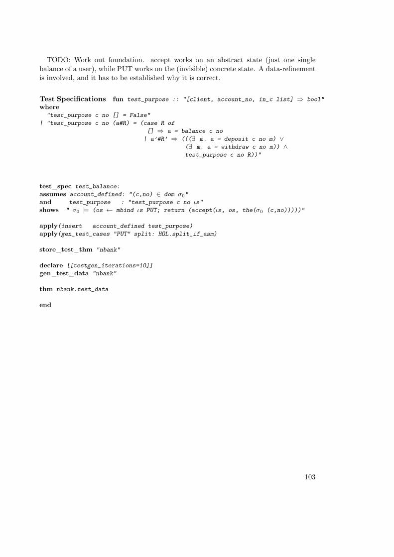
TODO: Work out foundation. accept works on an abstract state (just one singlebalance of a user), while PUT works on the (invisible) concrete state. A data-refinementis involved, and it has to be established why it is correct.
Test Specifications fun test_purpose :: "[client, account_no, in_c list] ⇒ bool"
where"test_purpose c no [] = False"
| "test_purpose c no (a#R) = (case R of
[] ⇒ a = balance c no
| a’#R’ ⇒ (((∃ m. a = deposit c no m) ∨(∃ m. a = withdraw c no m)) ∧test_purpose c no R))"
test spec test_balance:
assumes account_defined: "(c,no) ∈ dom σ0"
and test_purpose : "test_purpose c no ιs"shows " σ0 |= (os ← mbind ιs PUT; return (accept(ιs, os, the(σ0 (c,no)))))"
apply(insert account_defined test_purpose)
apply(gen_test_cases "PUT" split: HOL.split_if_asm)
store test thm "nbank"
declare [[testgen_iterations=10]]
gen test data "nbank"
thm nbank.test_data
end
103

A. Glossary
Abstract test data : In contrast to pure ground terms over constants (like integers1, 2, 3, or lists over them, or strings ...) abstract test data contain arbitrary predi-cate symbols (like triangle 3 4 5 ).
Regression testing: Repeating of tests after addition/bug fixes have been introducedinto the code and checking that behavior of unchanged portions has not changed.
Stub: Stubs are “simulated” implementations of functions, they are used to simulatefunctionality that does not yet exist ore cannot be run in the test environment.
Test case: An abstract test stimuli that tests some aspects of the implementation andvalidates the result.
Test case generation: For each operation the pre/postcondition relation is dividedinto sub-relations. It assumes that all members of a sub-relation lead to a similarbehavior of the implementation.
Test data: One or more representative for a given test case.
Test data generation (Test data selection): For each test case (at least) one rep-resentative is chosen so that coverage of all test cases is achieved. From the result-ing test data, test input data processable by the implementation is extracted.
Test execution: The implementation is run with the selected test input data in orderto determine the test output data.
Test executable: An executable program that consists of a test harness, the test scriptand the program under test. The Test executable executes the test and writes atest trace documenting the events and the outcome of the test.
Test harness: When doing unit testing the program under test is not a runnable pro-gram in itself. The test harness or test driver is a main program that initiatestest calls (controlled by the test script), i. e. drives the method under test andconstitutes a test executable together with the test script and the program undertest.
Test hypothesis : The hypothesis underlying a test that makes a successful test equiv-alent to the validity of the tested property, the test specification. The current im-plementation of HOL-TestGen only supports uniformity and regularity hypotheses,which are generated “on-the-fly” according to certain parameters given by the userlike depth and breadth.
105
Test specification : The property the program under test is required to have.
Test result verification: The pair of input/output data is checked against the speci-fication of the test case.
Test script: The test program containing the control logic that drives the test usingthe test harness. HOL-TestGen can automatically generate the test script for youbased on the generated test data.
Test theorem: The test data together with the test hypothesis will imply the testspecification. HOL-TestGen conservatively computes a theorem of this form thatrelates testing explicitly with verification.
Test trace: Output made by a test executable.
106
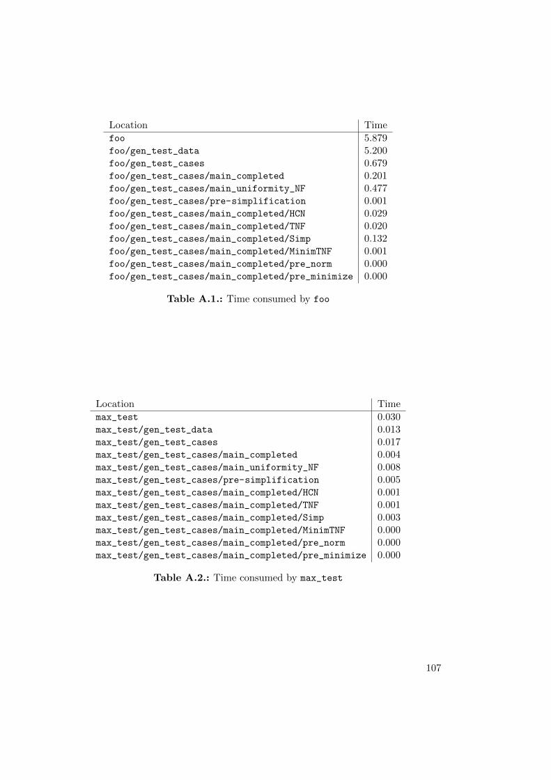
Location Time
foo 5.879foo/gen_test_data 5.200foo/gen_test_cases 0.679foo/gen_test_cases/main_completed 0.201foo/gen_test_cases/main_uniformity_NF 0.477foo/gen_test_cases/pre-simplification 0.001foo/gen_test_cases/main_completed/HCN 0.029foo/gen_test_cases/main_completed/TNF 0.020foo/gen_test_cases/main_completed/Simp 0.132foo/gen_test_cases/main_completed/MinimTNF 0.001foo/gen_test_cases/main_completed/pre_norm 0.000foo/gen_test_cases/main_completed/pre_minimize 0.000
Table A.1.: Time consumed by foo
Location Time
max_test 0.030max_test/gen_test_data 0.013max_test/gen_test_cases 0.017max_test/gen_test_cases/main_completed 0.004max_test/gen_test_cases/main_uniformity_NF 0.008max_test/gen_test_cases/pre-simplification 0.005max_test/gen_test_cases/main_completed/HCN 0.001max_test/gen_test_cases/main_completed/TNF 0.001max_test/gen_test_cases/main_completed/Simp 0.003max_test/gen_test_cases/main_completed/MinimTNF 0.000max_test/gen_test_cases/main_completed/pre_norm 0.000max_test/gen_test_cases/main_completed/pre_minimize 0.000
Table A.2.: Time consumed by max_test
107
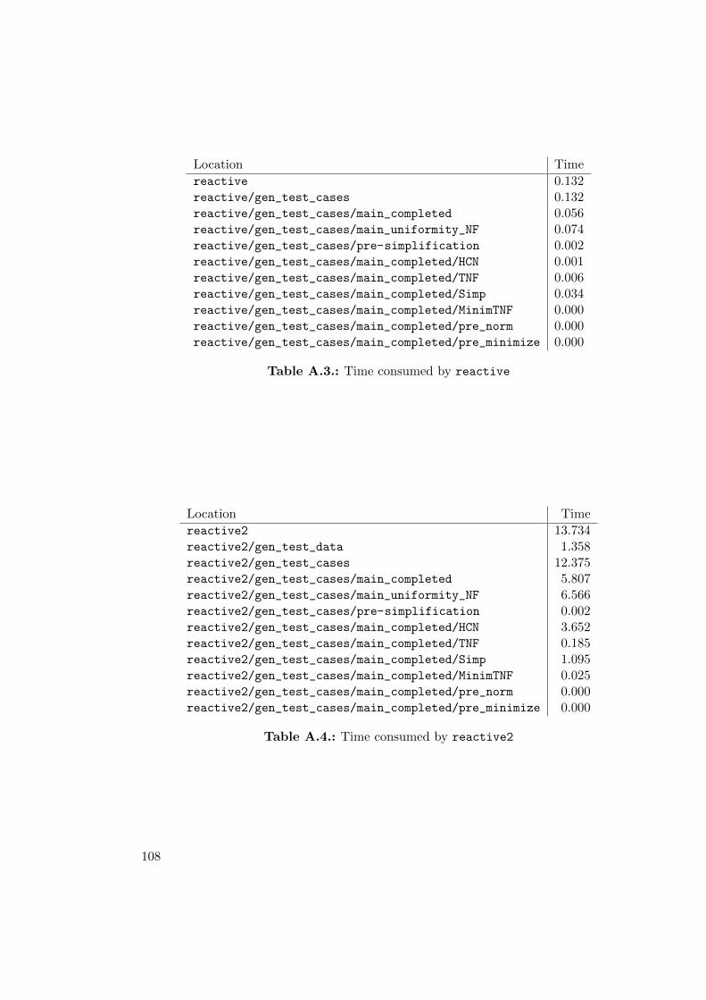
Location Time
reactive 0.132reactive/gen_test_cases 0.132reactive/gen_test_cases/main_completed 0.056reactive/gen_test_cases/main_uniformity_NF 0.074reactive/gen_test_cases/pre-simplification 0.002reactive/gen_test_cases/main_completed/HCN 0.001reactive/gen_test_cases/main_completed/TNF 0.006reactive/gen_test_cases/main_completed/Simp 0.034reactive/gen_test_cases/main_completed/MinimTNF 0.000reactive/gen_test_cases/main_completed/pre_norm 0.000reactive/gen_test_cases/main_completed/pre_minimize 0.000
Table A.3.: Time consumed by reactive
Location Time
reactive2 13.734reactive2/gen_test_data 1.358reactive2/gen_test_cases 12.375reactive2/gen_test_cases/main_completed 5.807reactive2/gen_test_cases/main_uniformity_NF 6.566reactive2/gen_test_cases/pre-simplification 0.002reactive2/gen_test_cases/main_completed/HCN 3.652reactive2/gen_test_cases/main_completed/TNF 0.185reactive2/gen_test_cases/main_completed/Simp 1.095reactive2/gen_test_cases/main_completed/MinimTNF 0.025reactive2/gen_test_cases/main_completed/pre_norm 0.000reactive2/gen_test_cases/main_completed/pre_minimize 0.000
Table A.4.: Time consumed by reactive2
108
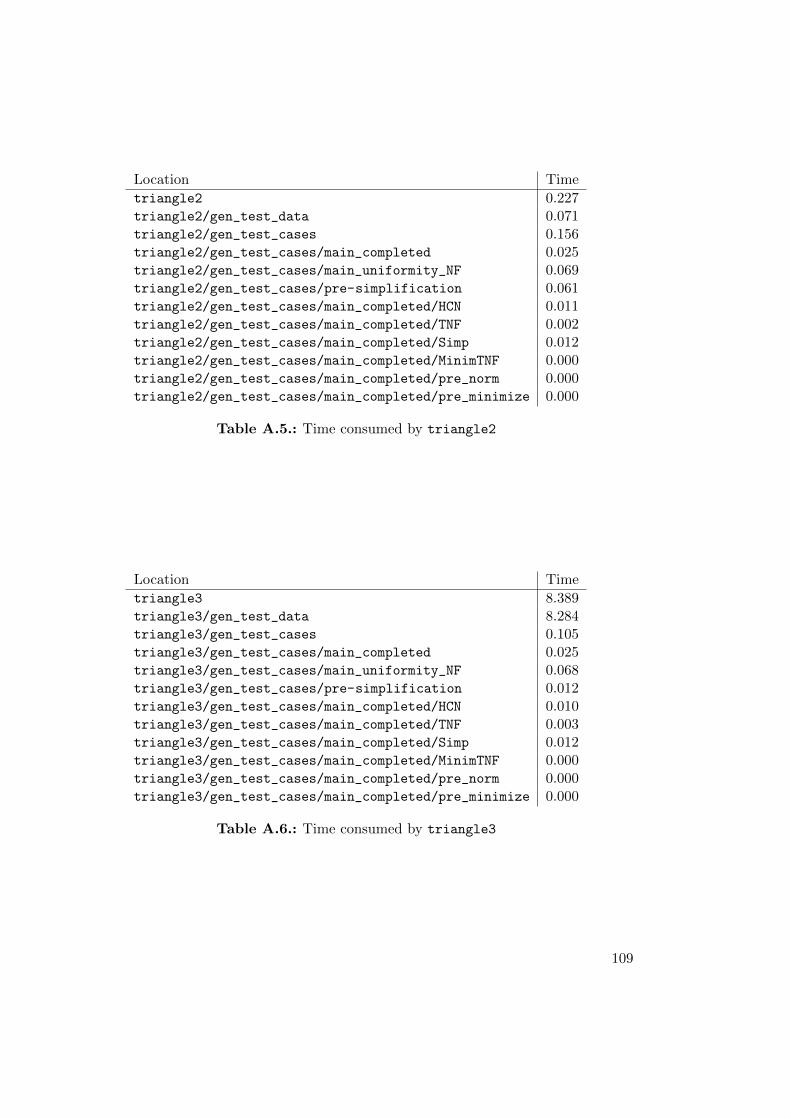
Location Time
triangle2 0.227triangle2/gen_test_data 0.071triangle2/gen_test_cases 0.156triangle2/gen_test_cases/main_completed 0.025triangle2/gen_test_cases/main_uniformity_NF 0.069triangle2/gen_test_cases/pre-simplification 0.061triangle2/gen_test_cases/main_completed/HCN 0.011triangle2/gen_test_cases/main_completed/TNF 0.002triangle2/gen_test_cases/main_completed/Simp 0.012triangle2/gen_test_cases/main_completed/MinimTNF 0.000triangle2/gen_test_cases/main_completed/pre_norm 0.000triangle2/gen_test_cases/main_completed/pre_minimize 0.000
Table A.5.: Time consumed by triangle2
Location Time
triangle3 8.389triangle3/gen_test_data 8.284triangle3/gen_test_cases 0.105triangle3/gen_test_cases/main_completed 0.025triangle3/gen_test_cases/main_uniformity_NF 0.068triangle3/gen_test_cases/pre-simplification 0.012triangle3/gen_test_cases/main_completed/HCN 0.010triangle3/gen_test_cases/main_completed/TNF 0.003triangle3/gen_test_cases/main_completed/Simp 0.012triangle3/gen_test_cases/main_completed/MinimTNF 0.000triangle3/gen_test_cases/main_completed/pre_norm 0.000triangle3/gen_test_cases/main_completed/pre_minimize 0.000
Table A.6.: Time consumed by triangle3
109
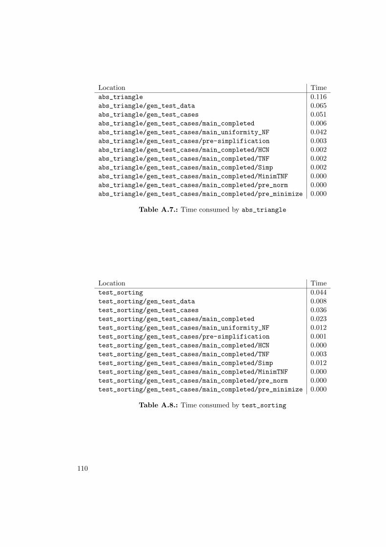
Location Time
abs_triangle 0.116abs_triangle/gen_test_data 0.065abs_triangle/gen_test_cases 0.051abs_triangle/gen_test_cases/main_completed 0.006abs_triangle/gen_test_cases/main_uniformity_NF 0.042abs_triangle/gen_test_cases/pre-simplification 0.003abs_triangle/gen_test_cases/main_completed/HCN 0.002abs_triangle/gen_test_cases/main_completed/TNF 0.002abs_triangle/gen_test_cases/main_completed/Simp 0.002abs_triangle/gen_test_cases/main_completed/MinimTNF 0.000abs_triangle/gen_test_cases/main_completed/pre_norm 0.000abs_triangle/gen_test_cases/main_completed/pre_minimize 0.000
Table A.7.: Time consumed by abs_triangle
Location Time
test_sorting 0.044test_sorting/gen_test_data 0.008test_sorting/gen_test_cases 0.036test_sorting/gen_test_cases/main_completed 0.023test_sorting/gen_test_cases/main_uniformity_NF 0.012test_sorting/gen_test_cases/pre-simplification 0.001test_sorting/gen_test_cases/main_completed/HCN 0.000test_sorting/gen_test_cases/main_completed/TNF 0.003test_sorting/gen_test_cases/main_completed/Simp 0.012test_sorting/gen_test_cases/main_completed/MinimTNF 0.000test_sorting/gen_test_cases/main_completed/pre_norm 0.000test_sorting/gen_test_cases/main_completed/pre_minimize 0.000
Table A.8.: Time consumed by test_sorting
110
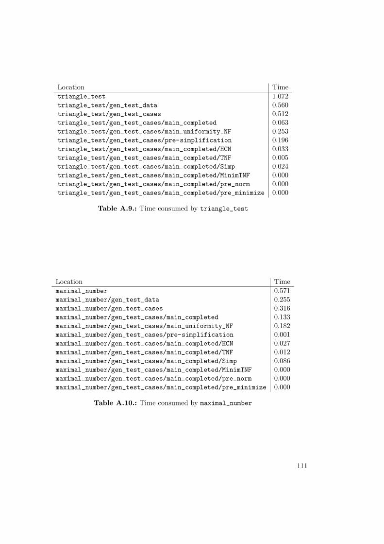
Location Time
triangle_test 1.072triangle_test/gen_test_data 0.560triangle_test/gen_test_cases 0.512triangle_test/gen_test_cases/main_completed 0.063triangle_test/gen_test_cases/main_uniformity_NF 0.253triangle_test/gen_test_cases/pre-simplification 0.196triangle_test/gen_test_cases/main_completed/HCN 0.033triangle_test/gen_test_cases/main_completed/TNF 0.005triangle_test/gen_test_cases/main_completed/Simp 0.024triangle_test/gen_test_cases/main_completed/MinimTNF 0.000triangle_test/gen_test_cases/main_completed/pre_norm 0.000triangle_test/gen_test_cases/main_completed/pre_minimize 0.000
Table A.9.: Time consumed by triangle_test
Location Time
maximal_number 0.571maximal_number/gen_test_data 0.255maximal_number/gen_test_cases 0.316maximal_number/gen_test_cases/main_completed 0.133maximal_number/gen_test_cases/main_uniformity_NF 0.182maximal_number/gen_test_cases/pre-simplification 0.001maximal_number/gen_test_cases/main_completed/HCN 0.027maximal_number/gen_test_cases/main_completed/TNF 0.012maximal_number/gen_test_cases/main_completed/Simp 0.086maximal_number/gen_test_cases/main_completed/MinimTNF 0.000maximal_number/gen_test_cases/main_completed/pre_norm 0.000maximal_number/gen_test_cases/main_completed/pre_minimize 0.000
Table A.10.: Time consumed by maximal_number
111
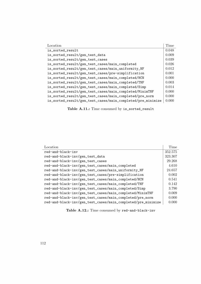
Location Time
is_sorted_result 0.048is_sorted_result/gen_test_data 0.009is_sorted_result/gen_test_cases 0.039is_sorted_result/gen_test_cases/main_completed 0.026is_sorted_result/gen_test_cases/main_uniformity_NF 0.012is_sorted_result/gen_test_cases/pre-simplification 0.001is_sorted_result/gen_test_cases/main_completed/HCN 0.000is_sorted_result/gen_test_cases/main_completed/TNF 0.003is_sorted_result/gen_test_cases/main_completed/Simp 0.014is_sorted_result/gen_test_cases/main_completed/MinimTNF 0.000is_sorted_result/gen_test_cases/main_completed/pre_norm 0.000is_sorted_result/gen_test_cases/main_completed/pre_minimize 0.000
Table A.11.: Time consumed by is_sorted_result
Location Time
red-and-black-inv 352.575red-and-black-inv/gen_test_data 323.307red-and-black-inv/gen_test_cases 29.268red-and-black-inv/gen_test_cases/main_completed 4.610red-and-black-inv/gen_test_cases/main_uniformity_NF 24.657red-and-black-inv/gen_test_cases/pre-simplification 0.002red-and-black-inv/gen_test_cases/main_completed/HCN 0.541red-and-black-inv/gen_test_cases/main_completed/TNF 0.142red-and-black-inv/gen_test_cases/main_completed/Simp 3.790red-and-black-inv/gen_test_cases/main_completed/MinimTNF 0.009red-and-black-inv/gen_test_cases/main_completed/pre_norm 0.000red-and-black-inv/gen_test_cases/main_completed/pre_minimize 0.000
Table A.12.: Time consumed by red-and-black-inv
112
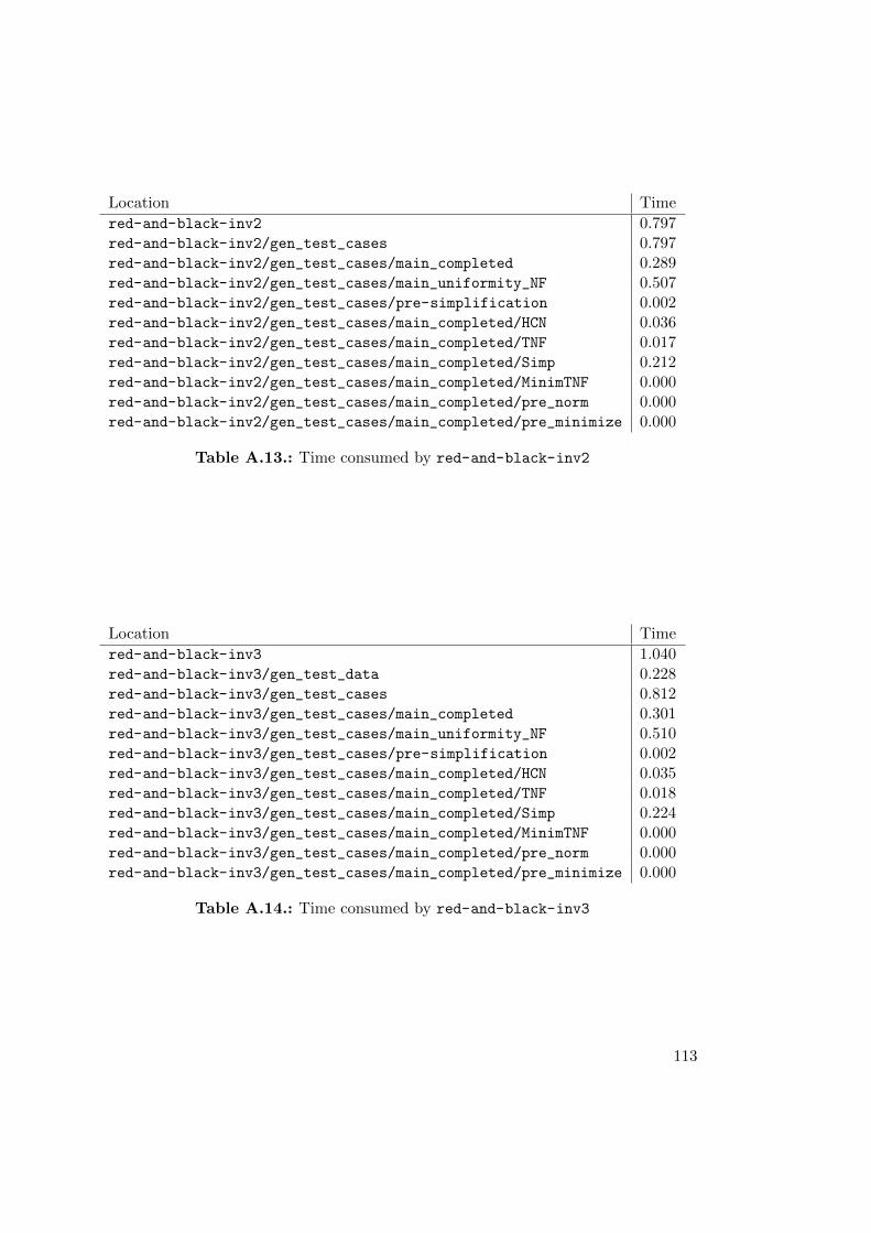
Location Time
red-and-black-inv2 0.797red-and-black-inv2/gen_test_cases 0.797red-and-black-inv2/gen_test_cases/main_completed 0.289red-and-black-inv2/gen_test_cases/main_uniformity_NF 0.507red-and-black-inv2/gen_test_cases/pre-simplification 0.002red-and-black-inv2/gen_test_cases/main_completed/HCN 0.036red-and-black-inv2/gen_test_cases/main_completed/TNF 0.017red-and-black-inv2/gen_test_cases/main_completed/Simp 0.212red-and-black-inv2/gen_test_cases/main_completed/MinimTNF 0.000red-and-black-inv2/gen_test_cases/main_completed/pre_norm 0.000red-and-black-inv2/gen_test_cases/main_completed/pre_minimize 0.000
Table A.13.: Time consumed by red-and-black-inv2
Location Time
red-and-black-inv3 1.040red-and-black-inv3/gen_test_data 0.228red-and-black-inv3/gen_test_cases 0.812red-and-black-inv3/gen_test_cases/main_completed 0.301red-and-black-inv3/gen_test_cases/main_uniformity_NF 0.510red-and-black-inv3/gen_test_cases/pre-simplification 0.002red-and-black-inv3/gen_test_cases/main_completed/HCN 0.035red-and-black-inv3/gen_test_cases/main_completed/TNF 0.018red-and-black-inv3/gen_test_cases/main_completed/Simp 0.224red-and-black-inv3/gen_test_cases/main_completed/MinimTNF 0.000red-and-black-inv3/gen_test_cases/main_completed/pre_norm 0.000red-and-black-inv3/gen_test_cases/main_completed/pre_minimize 0.000
Table A.14.: Time consumed by red-and-black-inv3
113
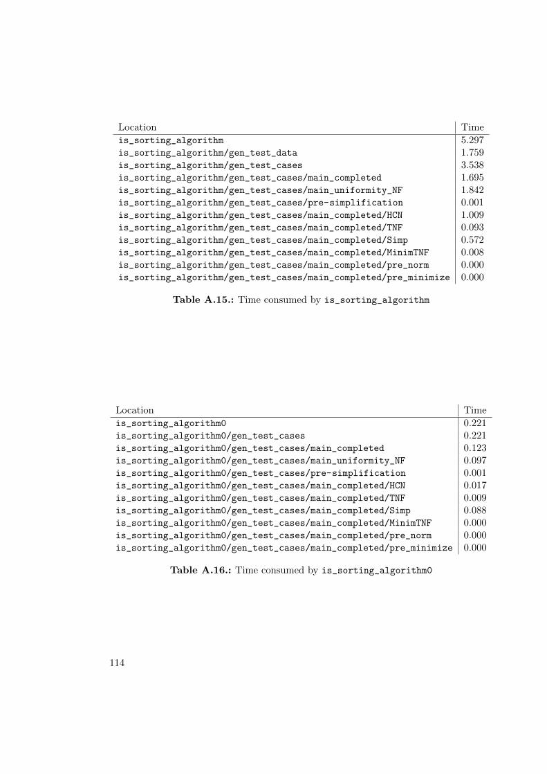
Location Time
is_sorting_algorithm 5.297is_sorting_algorithm/gen_test_data 1.759is_sorting_algorithm/gen_test_cases 3.538is_sorting_algorithm/gen_test_cases/main_completed 1.695is_sorting_algorithm/gen_test_cases/main_uniformity_NF 1.842is_sorting_algorithm/gen_test_cases/pre-simplification 0.001is_sorting_algorithm/gen_test_cases/main_completed/HCN 1.009is_sorting_algorithm/gen_test_cases/main_completed/TNF 0.093is_sorting_algorithm/gen_test_cases/main_completed/Simp 0.572is_sorting_algorithm/gen_test_cases/main_completed/MinimTNF 0.008is_sorting_algorithm/gen_test_cases/main_completed/pre_norm 0.000is_sorting_algorithm/gen_test_cases/main_completed/pre_minimize 0.000
Table A.15.: Time consumed by is_sorting_algorithm
Location Time
is_sorting_algorithm0 0.221is_sorting_algorithm0/gen_test_cases 0.221is_sorting_algorithm0/gen_test_cases/main_completed 0.123is_sorting_algorithm0/gen_test_cases/main_uniformity_NF 0.097is_sorting_algorithm0/gen_test_cases/pre-simplification 0.001is_sorting_algorithm0/gen_test_cases/main_completed/HCN 0.017is_sorting_algorithm0/gen_test_cases/main_completed/TNF 0.009is_sorting_algorithm0/gen_test_cases/main_completed/Simp 0.088is_sorting_algorithm0/gen_test_cases/main_completed/MinimTNF 0.000is_sorting_algorithm0/gen_test_cases/main_completed/pre_norm 0.000is_sorting_algorithm0/gen_test_cases/main_completed/pre_minimize 0.000
Table A.16.: Time consumed by is_sorting_algorithm0
114
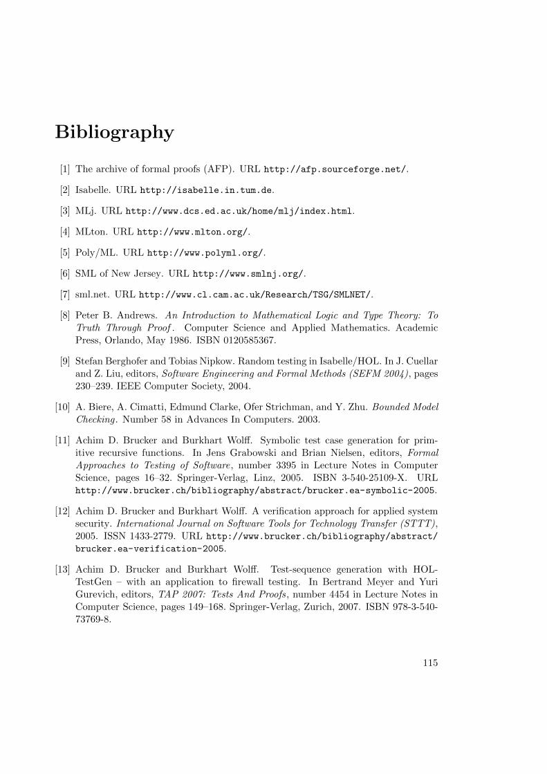
Bibliography
[1] The archive of formal proofs (AFP). URL http://afp.sourceforge.net/.
[2] Isabelle. URL http://isabelle.in.tum.de.
[3] MLj. URL http://www.dcs.ed.ac.uk/home/mlj/index.html.
[4] MLton. URL http://www.mlton.org/.
[5] Poly/ML. URL http://www.polyml.org/.
[6] SML of New Jersey. URL http://www.smlnj.org/.
[7] sml.net. URL http://www.cl.cam.ac.uk/Research/TSG/SMLNET/.
[8] Peter B. Andrews. An Introduction to Mathematical Logic and Type Theory: ToTruth Through Proof . Computer Science and Applied Mathematics. AcademicPress, Orlando, May 1986. ISBN 0120585367.
[9] Stefan Berghofer and Tobias Nipkow. Random testing in Isabelle/HOL. In J. Cuellarand Z. Liu, editors, Software Engineering and Formal Methods (SEFM 2004), pages230–239. IEEE Computer Society, 2004.
[10] A. Biere, A. Cimatti, Edmund Clarke, Ofer Strichman, and Y. Zhu. Bounded ModelChecking . Number 58 in Advances In Computers. 2003.
[11] Achim D. Brucker and Burkhart Wolff. Symbolic test case generation for prim-itive recursive functions. In Jens Grabowski and Brian Nielsen, editors, FormalApproaches to Testing of Software, number 3395 in Lecture Notes in ComputerScience, pages 16–32. Springer-Verlag, Linz, 2005. ISBN 3-540-25109-X. URLhttp://www.brucker.ch/bibliography/abstract/brucker.ea-symbolic-2005.
[12] Achim D. Brucker and Burkhart Wolff. A verification approach for applied systemsecurity. International Journal on Software Tools for Technology Transfer (STTT),2005. ISSN 1433-2779. URL http://www.brucker.ch/bibliography/abstract/
brucker.ea-verification-2005.
[13] Achim D. Brucker and Burkhart Wolff. Test-sequence generation with HOL-TestGen – with an application to firewall testing. In Bertrand Meyer and YuriGurevich, editors, TAP 2007: Tests And Proofs, number 4454 in Lecture Notes inComputer Science, pages 149–168. Springer-Verlag, Zurich, 2007. ISBN 978-3-540-73769-8.
115

[14] Achim D. Brucker and Burkhart Wolff. HOL-TestGen: An interactive test-case gen-eration framework. In Marsha Chechik and Martin Wirsing, editors, FundamentalApproaches to Software Engineering (FASE09), number 5503 in Lecture Notes inComputer Science, pages 417–420. Springer-Verlag, Heidelberg, 2009. URL http:
//www.brucker.ch/bibliography/abstract/brucker.ea-hol-testgen-2009.
[15] Achim D. Brucker and Burkhart Wolff. On theorem prover-based testing. FormalAspects of Computing , 2012. ISSN 0934-5043. URL http://www.brucker.ch/
bibliography/abstract/brucker.ea-theorem-prover-2012.
[16] Alonzo Church. A formulation of the simple theory of types. Journal of SymbolicLogic, 5:56–68, 1940.
[17] Koen Claessen and John Hughes. QuickCheck: a lightweight tool for random test-ing of Haskell programs. In Proceedings of the fifth ACM SIGPLAN internationalconference on Functional programming , pages 268–279. ACM Press, 2000. ISBN1-58113-202-6.
[18] Patrick Cousot and Radhia Cousot. Abstract interpretation: a unified lattice modelfor static analysis of programs by construction or approximation of fixpoints. InProceedings of the 4th ACM SIGACT-SIGPLAN symposium on Principles of pro-gramming languages, pages 238–252. ACM Press, 1977.
[19] O.-J. Dahl, E. W. Dijkstra, and C. A. R. Hoare. Structured Programming , volume 8of A.P.I.C. Studies in Data Processing . Academic Press, London, 1972. ISBN 0-12-200550-3.
[20] Jeremy Dick and Alain Faivre. Automating the generation and sequencing of testcases from model-based specications. In J.C.P. Woodcock and P.G. Larsen, editors,Formal Methods Europe 93: Industrial-Strength Formal Methods, volume 670 ofLNCS , pages 268–284. Springer, April 1993.
[21] Peter Dybjer, Qiao Haiyan, and Makoto Takeyama. Verifying haskell programs bycombining testing and proving. In Proceedings of the Third International Confer-ence on Quality Software, page 272. IEEE Computer Society, 2003. ISBN 0-7695-2015-4. URL http://csdl.computer.org/comp/proceedings/qsic/2003/2015/
00/20150272abs.htm.
[22] Marie-Claude Gaudel. Testing can be formal, too. In Peter D. Mosses, MogensNielsen, and Michael I. Schwartzbach, editors, TAPSOFT 95 , volume 915 of LectureNotes in Computer Science, pages 82–96. Springer-Verlag, Aarhus, Denmark, 1995.ISBN 3-540-59293-8.
[23] Susumu Hayashi. Towards the animation of proofs—testing proofs by examples.Theoretical Computer Science, 272(1–2):177–195, 2002.
116
[24] Tobias Nipkow, Lawrence C. Paulson, and Markus Wenzel. Isabelle/HOL — AProof Assistant for Higher-Order Logic, volume 2283 of LNCS . Springer, 2002.URL http://www4.in.tum.de/~nipkow/LNCS2283/.
[25] N. D. North. Automatic test generation for the triangle problem. Technical ReportDITC 161/90, National Physical Laboratory, Teddington, Middlesex TW11 0LW,UK, February 1990.
[26] Markus Wenzel. The Isabelle/Isar Reference Manual . TU Munchen, Munchen,2004. URL http://isabelle.in.tum.de/dist/Isabelle2004/doc/isar-ref.
pdf.
[27] Hong Zhu, Patrick A.V. Hall, and John H. R. May. Software unit test coverage andadequacy. ACM Computing Surveys, 29(4):366–427, 1997. ISSN 0360-0300.
117

Index
symbolsRSF. . . . . . . . . . . . . . . . . . . . . . . . . . . . . . . . .16
Aabstract test case . . . . . . . . . . . . . . . . . . . .52
abstract test data . . . . . . . . . . . . . . . . . . 105
Bbreadth . . . . . . . . . . . . . . . . . . . . . . . . . . . . 105
〈breadth〉 . . . . . . . . . . . . . . . . . . . . . . . . . . . . 15
C〈clasimpmod〉 . . . . . . . . . . . . . . . . . . . . . . . 15
Ddata separation lemma . . . . . . . . . . . . . . 15
depth . . . . . . . . . . . . . . . . . . . . . . . . . . . . . . 105
〈depth〉 . . . . . . . . . . . . . . . . . . . . . . . . . . . . . . 15
Eexport test data (command) . . . . . 16
Ggen test cases (method) . . . . . . . . . 15
gen test data (command) . . . . . . . . 16
generate test script (command) 17
Hhigher-order logic . . . . . . . . . . . . . see HOL
HOL . . . . . . . . . . . . . . . . . . . . . . . . . . . . . . . . . 7
IIsabelle . . . . . . . . . . . . . . . . . . . . . . . . . .6, 7, 9
MMain (theory) . . . . . . . . . . . . . . . . . . . . . . . 13
N〈name〉 . . . . . . . . . . . . . . . . . . . . . . . . . . . . . . 16
Pprogram under test . . . . . . . . . . . . . . . . . . 50program under test . . . . . . . . . . . . . . 15, 17
Rrandom solve failure . . . . . . . . . . . . see RSF
random solver . . . . . . . . . . . . . . . . . . . 16, 47regression testing . . . . . . . . . . . . . . . . . . .105regularity hypothesis . . . . . . . . . . . . . . . . 15
SSML . . . . . . . . . . . . . . . . . . . . . . . . . . . . . . . . . 7software
testing . . . . . . . . . . . . . . . . . . . . . . . . . . . 5validation . . . . . . . . . . . . . . . . . . . . . . . . 5verification . . . . . . . . . . . . . . . . . . . . . . . 5
Standard ML . . . . . . . . . . . . . . . . . see SMLstore test thm (command) . . . . . . . 15stub. . . . . . . . . . . . . . . . . . . . . . . . . . . . . . . .105
Ttest . . . . . . . . . . . . . . . . . . . . . . . . . . . . . . . . . . 6test (attribute) . . . . . . . . . . . . . . . . . . . . . 19test specification . . . . . . . . . . . . . . . . . . . . 13test theorem . . . . . . . . . . . . . . . . . . . . . . . . 16test case. . . . . . . . . . . . . . . . . . . . . . . . . . . . .13test data generation . . . . . . . . . . . . . . . . . 13test executable . . . . . . . . . . . . . . . . . . . . . . 13test specification. . . . . . . . . . . . . . . . . . . . . .6test case . . . . . . . . . . . . . . . . . . . . . . . . . 6, 105test case generation . . . 5, 13, 15, 19, 105test data . . . . . . . . . . . . . . . . . 6, 13, 16, 105test data generation . . . . . . . . . . . . . 6, 105
119
test data selection. . . . . . . . .see test datageneration
test driver . . . . . . . . . . . . .see test harnesstest environment . . . . . . . . . . . . . . . . . . . . 51test executable . . . . . . . . . . . . . . 19–21, 105test execution . . . . . . . . . . . . 6, 13, 19, 105test harness . . . . . . . . . . . . . . . . . . . . 17, 105test hypothesis . . . . . . . . . . . . . . . . . . 6, 105test procedure . . . . . . . . . . . . . . . . . . . . . . . . 5test result verification . . . . . . . . . . . . . . . 13test result verification. . . . . . . . . . . .6, 106test script . . . . . . . . . . . . . . . 13, 17, 19, 106test specification. . . . . . . . . . . . . . . .15, 106test theorem. . . . . . . . . . . . . . . . . . . . 51, 106test theory . . . . . . . . . . . . . . . . . . . . . . . . . . 14test trace . . . . . . . . . . . . . . . . . . . 20, 21, 106test spec (command). . . . . . . . . . . . . . .13testgen params (command) . . . . . . . . 17Testing (theory) . . . . . . . . . . . . . . . . . . . . 13
Uunit test
specification-based . . . . . . . . . . . . . . . 5
120