Technology shocks andthe business cycle

Martin Eichenbaum

Historically, much research inmacroeconomics has focusedon assessing the relative im-portance of different shocks toaggregate economic activity.

The traditional view, shared by Monetaristsand Keynesians alike, is that exogenous shocksto aggregate demand, such as those induced byshifts in monetary policy, are central impulsesto the business cycle. Irrespective of theirother differences, adherents of the traditionalview share the common goal of striving tounderstand the mechanisms by which mone-tary policy affects aggregate economic activ-ity.

The repeated oil shocks of the last 15years and the accelerating pace of technologi-cal change have led to a breakdown in theconsensus that changes in aggregate demandare the main sources of business cycles. Thedecline of the traditional view coincided withthe development of a group of models, collec-tively known as Real Business Cycle (RBC)theories. In sharp contrast to the traditionalview, RBC theories seek to explain the busi-ness cycle in ways that abstract from monetaryconsiderations entirely. According to thesetheories, exogenous shocks to aggregate sup-ply, such as technology shocks, are the criticalsource of impulses to postwar U.S. businesscycles. While RBC theorists do not claim thatmonetary policy is inherently neutral, they dobelieve that RBC models can capture the sali-ent features of postwar U.S. business cycleswithout incorporating monetary shocks intothe analysis.

Pursuing such a strategy, Kydland andPrescott (1982) were able to construct andanalyze a simple general equilibrium model ofthe U.S. economy in which technology shockswere apparently able to account for all outputvariability in the postwar U.S. Building onKydland and Prescott's work, Hansen (1985)and other researchers showed that variants ofthe basic RBC model were also able to account for the relative volatility of key aggre-gate variables such as real consumption, in-vestment, and per capita hours worked. Giventhese findings, the need for an adequate theoryof monetary and fiscal sources of instabilityhas come to seem much less pressing. Perhapsas a consequence, the amount of research de-voted to these topics has declined precipi-tously.

Not surprisingly, RBC theories have gen-erated a great deal of controversy. In part, thiscontroversy revolves around the substantiveclaims made by RBC analysts. At the sametime there has been considerable controversyabout the fact that RBC analysts address thedata using highly stylized, general equilibriummodels.' Like all theoretical models, RBCmodels abstract from different aspects of real-

Martin Eichenbaum is professor of economics atNorthwestern University and senior consultant atthe Federal Reserve Bank of Chicago. The authorthanks Craig Burnside, Lawrence Christiano, SergioRebelo, Thomas Sargent, and Mark Watson fortheir advice and help. This article is based upon"Real business cycle theory: wisdom or whimsy?,"forthcoming, Journal of Economic Dynamics andControl.

14 ECONOMIC PERSPECTIVES

ity. According to this criticism, all theoreticalmodels, including RBC models, are wrong.While I agree that theoretical models are nec-essarily false, this criticism overlooks the realusefulness of many theoretical models. Whatis striking about RBC models is their apparentability to account for important features of thebusiness cycle, despite their obvious simplic-ity.

This article assesses the quality of theempirical evidence provided by RBC analyststo support their substantive claims regardingthe cyclical role of technology shocks. I arguethat the data and the methods used by theseanalysts are, in fact, almost completely unin-formative about the role of technology shocksin generating aggregate fluctuations in U.S.output. In addition I argue that their conclu-sions are not robust either to changes in thesample period investigated or to small pertur-bations in their models. For these reasons, Iconclude that the empirical results in the RBCliterature do not constitute a convincing chal-lenge to the traditional view regarding thecyclical importance of aggregate demandshocks.

The remainder of this article is organizedas follows. The second section summarizesthe evidence used by RBC analysts to supportthe claim that technology shocks account formost of the variability in aggregate U.S. out-put. I then argue that the empirical approachused by RBC analysts, commonly referred toas "calibration," does not provide useful inputinto the problem of deciding which impulseshave been the major sources of postwar fluc-tuations in output. The third section analyzesthe sensitivity of RBC conclusions to simpleperturbations in the model as well as tochanges in the sample period investigated.Finally, the fourth section contains some con-cluding remarks.

Technology shocks and aggregateoutput fluctuations

This section reviews the basic empiricalresults presented by RBC analysts to supporttheir contention that aggregate technologyshocks account for a large percentage of ag-gregate U.S. output fluctuations. In presentingthese results I abandon the RBC analysts'counterfactual assumption that the value of themodel's structural parameters are actuallyknown, rather than estimated. I then show that

the strong conclusions which mark the RBCliterature depend critically on this assumption.Absent this crucial assumption, the sharp infer-ences which RBC analysts draw regarding theimportance of technology shocks are not sup-ported by the data. I conclude that althoughtechnology shocks almost certainly play somerole in generating the business cycle, there issimply an enormous amount of uncertaintyabout just what percentage of aggregate fluc-tuations they actually do account for. Theanswer could be 70 percent as Kydland andPrescott (1989) claim, but it could also be 5percent or even 200 percent.

A prototypical Real BusinessCycle Model

RBC models share the view that aggregateeconomic time series correspond to the evolu-tion of a dynamic stochastic equilibrium inwhich optimizing firms, labor suppliers, andconsumers interact in stochastic environments.The basic sources of uncertainty in agents'environments constitute the impulses to thebusiness cycle. The type of impulse which hasreceived the most attention are shocks to theaggregate production technology which affectboth the marginal productivity of labor and themarginal productivity of capital.

Under these circumstances the time serieson hours worked and the return to workingcorrespond to the intersection of a stochasticlabor demand curve with a fixed labor supplycurve.' As long as agents are willing to substi-tute labor over time, an increase in the time tmarginal productivity of labor ought to gener-ate an increase in per capita hours worked, realwages, and output. Given a temporary in-crease in aggregate output and a desire onagents' part to smooth consumption over time,these theories also predict a large positiveincrease in investment as well as a positive butsmaller increase in consumption.

In order to assess the quantitative implica-tions of RBC theories it is useful to focus ourattention on one widely used RBC model—theIndivisible Labor Model associated with GaryHansen (1985) and Richard Rogerson (1988).The basic setup of that model can be describedas follows. The economy is populated by afinite number of infinitely lived, identical,perfectly competitive individuals. Each per-son is endowed with T units of time which canbe allocated towards work or leisure. To go to

FEDERAL RESERVE BANK OF CHICAGO 15

work, a person must incur a fixed cost,denominated in terms of hours of foregoneleisure. The length of the workday per se issome constant, say f hours, so that a workingperson has (T –f–) hours of leisure. An unem-ployed person has T hours of leisure. Indi-viduals care about leisure and consumption atdifferent points in time. Consequently, laborsupply behavior depends on a number of fac-tors. First, the typical individual cares aboutthe current return to working versus takingleisure. In the typical model, a higher realwage rate today implies that more people wishto work today, that is, labor suppliers are will-ing to substitute consumption for leisure. Sec-ond, current labor supply also depends on thereturns to working today versus the returns toworking in the future. In the typical modelthis means that, in response to a temporarilyhigh wage rate today, more people wish towork today, that is, labor suppliers are willingto engage in intertemporal substitution ofleisure and consumption.

According to the model, perfectly com-petitive firms combine labor services andcapital to produce a single storable good whichis sold in competitive markets. The good canbe consumed immediately or used as capitalone period later. An important feature of themodel is that firms' production technologiesare subject to stochastic technology shocks.For example, a positive technology shockincreases the marginal productivity of bothcapital and labor. Other things equal, such ashock would increase firms' demand for laborand capital. In the typical model, the technol-ogy shock is modeled as a stationary autore-gressive process which displays positive serialcorrelation. This means that positive technol-ogy shocks are expected to persist over time,although not permanently. The assumptionthat technology shocks are not permanent isparticularly important for the model's labormarket implications. If the shocks were per-manent, the marginal productivity of labor andthe return to working would be permanentlyhigher. Other things equal, this would chokeoff the incentive for labor suppliers to in-tertemporally substitute leisure in response toan increase in the return to working. Theassumption that technology shocks are persis-tent is particularly important for the model'scapital market implications. It takes time forcapital investments to come to fruition. If the

technology shocks were completely transitory,the demand for investment goods would beunaffected by technology shocks.

Finally, the model supposes that, like tech-nology shocks, government purchases of goodsand services evolve according to a stationaryautoregressive process which displays positiveserial correlation. This means that a positiveshock to government purchases leads agents toexpect unusually high levels of governmentconsumption for some periods to come. Thehigher the present value of government con-sumption, the higher the perceived level oflump sum taxes faced by the typical individual.The resulting negative income effect translatesinto an increase in the aggregate supply of laborand therefore equilibrium employment andoutput.'

In sum, according to the model, agentsface two kinds of uncertainty—the level oftechnology and the level of government pur-chases. Shocks to these variables are the solesources of aggregate fluctuations. Positiveshocks to either of these variables tend to in-duce increases in aggregate output. The result-ing fluctuations in aggregate veal variables arenot purely transitory for two reasons. First, thepresence of capital tends to induce serial corre-lation in the endogenous variables of the model.Second, the exogenous variables—the state oftechnology and the level of government—areassumed to be serially correlated over time.The reader is referred to the Box for the precisedetails of the model.

Quantitative implications of the theory

In reporting the model's quantitative impli-cations I will make use of constructs known as"moments". These refer to certain characteris-tics of the data generating process, such as amean or a variance. Moments are classifiedaccording to their order. An nth order momentrefers to the expected value of an nth orderpolynomial function of the variables in ques-tion. An example of a first order momentwould be the unconditional expected value oftime t output, Ey e. Examples of second ordermoments of the output process are the uncondi-tional variance of y E[t-Eyt]2 , and the covari-ance between output at time t and time t--T,E[y–Eyt][yt-T–Eyt-T]. An example of a secondorder moment involving two variables would bethe covariance between time t output and time thours worked, E[yt-Eyt][nt-Ent].

16 ECONOMIC PERSPECTIVES

Suppose that we denote the model's struc-tural parameters by the vector IP. Given aparticular value for IP, it is straightforward todeduce the model's implications for a widevariety of moments which might be of interest.In practice RBC analysts have concentrated ontheir models' properties for a small set ofmoments which they argue describe the salientfeatures of the business cycle. The momentwhich has received the most attention is thestandard deviation of output, lay.4 RBC ana-lysts also report their models' implications forobjects like the standard deviations of con-sumption, investment, average productivity,and hours worked. While this list of momentsis by no means exhaustive, it is primarily onthese dimensions of the data that RBC analystshave claimed their major successes.

To quantify whether a model has suc-ceeded in accounting for some moment, RBCstudies condition their empirical analysis on aparticular value for IP, say T. The model'sprediction for some moment is then comparedto an estimate of the corresponding data mo-ment. The ratio between these two magni-tudes is referred to as the percent of the mo-ment in question for which the model ac-counts. For example, cOnsider the variance ofoutput. When RBC analysts say that themodel accounts for 100X percent of the vari-ance of output, what they mean is that, for thismoment, their model yields X equal to

( 1) = 272),„,

Here the numerator denotes the varianceof model output, calculated under the assump-tion that 'Is is equal to and the denominatordenotes an estimate of the variance of actualU.S. output. The claim that technology shocksaccount for most of the fluctuations in postwarU.S. output corresponds to the claim that X is alarge number, with the current estimate beingbetween .75 and 1.0, depending on exactlywhich RBC model is used.'

To evaluate these types of claims we ab-stract for the moment from issues like sensitiv-ity to perturbations in the theory or changes inthe sample period being considered. As deci-sion makers, we need to know how much con-fidence to place in statements like "The modelaccounts for X percent of the variability ofoutput." But to answer this question we needto know how sensitive X is to small perturba-

Ations in 'P. And in order to answer this ques-tion we must decide on what a small perturba-tion in 'A-Pis.

Unfortunately, the existing RBC literaturedoes not offer much help in answering thesequestions. This is because RBC analysts havenot used formal econometric methods, either atthe stage when model parameter values areselected, or at the stage when the fully par-ameterized model is compared to the dataInstead they use a variety of informal tech-niques, known as "calibration." Unfortu-nately, for diagnostic purposes, these tech-niques are not a satisfactory alternative toformal econometric methods. This is becauseobjects like X are random variables, and henceare subject to sample uncertainty. Calibrationtechniques ignore the sample uncertainty in-herent in such statistics. As a result, the cali-brator must remain mute in response to thequestion "How much confidence do we havethat the model accounts for 100X percent ofthe variance of output?"

That there is sampling uncertainty in ran-dom variables like X, follows from the fact thatthey are statistics in the sense defined byPrescott (1986), that is, they are real valuedfunctions of the data. In the case of X, theprecise form of that dependency is determinedjointly by the functions defining O d, 41, andcry2.(4). According to Equation (1), samplinguncertainty in any of these random variablesimplies the existence of sampling uncertaintyin X. In fact, all of these objects are randomvariables, subject to sampling uncertainty. Tosee this, consider first We do not know thetrue variance of U.S. output, ay2d. This a popu-lation moment which must be estimated viasome well defined function of the data. Sinceu'd is an estimate of cs2 it is a random variable,yd'subject to samplirrg uncertainty. Next con-sider, the vector tP, the estimated value of themodel's structural parameters. It too is a ran-dom variable subject to sampling uncertainty.To see this, consider an element of ‘11 like a, aparameter that governs the marginal physicalproductivity of labor. Calibrators typicallychoose a value for a, say a, which implies thatthe model reproduces the "observed" share oflabor in national income. But we do not ob-serve the population value of labor share innational income; this is an object which mustbe estimated via some function of the data.Since the estimator defined by that function is

FEDERAL RESERVE BANK OF CHICAGO 17

The Indivisible Labor Model: a prototypical Real Business Cycle Model .

The representative individual's time t utilitylevel depends on time t consumption, c1 , and time tleisure, If , in a way described by the function

(1) U(c, = u(ct) + v(1,).

The functions u and v are strictly increasing,concave functions of consumption and leisure,respectively. At time zero, the typical individualseeks to maximize the expected discounted value ofhis/her lifetime utility, that is,

CO

(2) E0 I lit U(ct, 1,),t=0

where E0 denotes the expectations operator condi-tional on the typical person's time zero informationset and 13 is a subjective discount rate between zeroand one.

The single consumption good in this economyis produced by perfectly competitive firms using aconstant returns to scale technology, F(kt, ),which relates the beginning of time t capital, k, ,total hours worked, n ,, and the time t stochasticlevel of technology, z1 , to total output. The stock ofcapital evolves according to

(3) k[+] = (1-5)k, + i 1

where it denotes time t gross investmentand 5 is the constant depreciation rate on capital,0 < 8 < 1.

In the aggregate, consumption plus grossinvestment plus government purchases of the goodcannot exceed current output, that is the economy issubject to the aggregate budget constraint,

(4) c, + k[+] — (1-8)k, + x, 5 y 1 .

The variable x, denotes time t governmentpurchases of the goods.

To derive the quantitative implications of thepreceding model we must specify the functionssummarizing preferences and technology, u, v, andF, as well as the laws of motion governing the evo-lution of the technology shocks and governmentpurchases. In addition we must be specific aboutthe market setting in which private agents interact.As in most existing RBC studies, we suppose thathouseholds and firms interact in perfectly competi-tive markets. As it turns out, deriving the competi-tive equilibrium of our model is greatly simplifiedif we exploit the well-known connection betweencompetitive equilibria and optimal allocations.This connection allows us to analyze a simple"social planning" problem whose solution happensto coincide with the competitive equilibrium of oureconomy.

In displaying the planning problem which isappropriate for our economy it is useful to firstmake explicit Hansen's assumptions regardingpreferences and technology. The function u(ct ) isassumed to be given by In(ct). Total time t output,y 1 , is assumed to be produced using the production

Asubject to sampling uncertainty, so too 4'. Itfollows that o2ym(tT), which depends on T, isalso a random variable, subject to samplinguncertainty.

The previous discussion indicates that allof the elements required to calculate A arerandom variables. Clearly A will inherit therandomness and sampling uncertainty in itsconstituent elements. Since calibration tech-niques treat the elements of A(6 y2e, 41, andcy2

m M) as fixed numbers, these techniques

ymust also treat A as a fixed number rather thanas a random variable. As a consequence, cali-bration techniques cannot be used to quantifythe sampling uncertainty inherent in an objectlike A. To do this, one must use formal econ-ometric methods.

In recent work, Lawrence Christiano and Idiscuss one way to quantify sampling uncer-tainty in the diagnostic statistics typically usedby RBC analysts. 6 The basic idea is to utilizea version of Hansen's (1982) GeneralizedMethod of Moments procedure in which theestimation criterion is set up so that, in effect,the estimated parameter values succeed inequating model and sample first order mo-ments of the data. It turns out that these val-ues are very similar to the values employed inexisting RBC studies. For example, most RBCstudies assume that the quarterly depreciationrate, 8, and the share of capital in the aggre-gate production function, (1—a), equal .025and .36, respectively.' Our procedure yieldspoint estimates of .021 and .35, respectively.

18 ECONOMIC PERSPECTIVES

function like n , , z,) = z, n,u. The technologyshock, z1 , evolves according to

(5) zt7' A t

= exp(e ).

Here A, is the stationary component of z,, pQ isa scalar satisfying I p,, I < 1, E is the time t innova-tion to 1n(A 1 ) with mean e and standard deviation0E . The parameter y is a positive constant whichgoverns growth in the economy.' In addition gov-ernment purchases are assumed to evolve accordingto

(6) x i = y tg i

= g ji exp(1.1 t )•

Here g 1 is the stationary stochastic componentof x,, p g is a scalar satisfying I [38 I < 1, and t is theinnovation in In(g,) with mean Ix and standarddeviation a .

Proceeding as in Hansen (1985) and Rogerson(1988) it can be shown that the competitive equilib-rium laws of motion for kr , c,, and n o, correspond tothe solution of a planning problem in whichstreams of consumption services and hours workedare ranked according to the criterion function:

00

(7) E0 E (ln(c,) + 0(T—n t ))t=0

where 0 is some positive scalar. The planner maxi-mizes (7) subject to the resource constraint

(8) c, + — (1 -8)k i + x t =

and the laws of motion for z, and x, given by (5)and (6).

There are at least two interpretations of theterm involving leisure in (7). First, it may justreflect the assumption that the function v(11) islinear in leisure. The second interpretation buildson the assumption that there are fixed costs ofgoing to work. Because of this individuals willeither work some fixed positive number of hours ornot at all. Assuming that agents' utility functionsare separable across consumption and leisure,Rogerson (1988) shows that a market structure inwhich individuals choose the probability of beingemployed rather than actual hours worked willsupport the Pareto optimal allocation. With thisinterpretation, equation (7) represents a reducedform preference ordering which can be used toderive the competitive equilibrium allocation.However, at the micro level of the individual agent,the parameter 0 places no restrictions on the elas-ticity of labor supply.

'Our model exhibits balanced growth, so that the log of allreal variables, excluding per capita hours worked, have anunconditional growth rate of y.

The key difference between the proce-dures does not lie so much in the point esti-mates ofii. Rather the difference is that, byusing formal econometrics, our procedureallows us to translate sampling uncertaintyabout the functions of the data which defineour estimator of 1' into sampling uncertaintyregarding kV itself. This information leads to anatural definition of what a small perturbationin It is. In turn this makes it possible to quan-tify uncertainty about the model's momentimplications.

Before reporting the results of implement-ing this procedure for the Indivisible LaborModel, I must digress for one moment anddiscuss the way in which growth is handled.In practice empirical measures of objects likey, display marked trends, so that some station-

ary inducing transformation of the data must beadopted. A variety of alternatives are availableto the analyst. For example, our setup impliesthat the data are realizations of a trend station-ary process, with the log of all real variables(excluding per capita hours worked) growing asa linear function of time. So one possibilitywould be to detrend the time series emergingfrom the model as well as the actual data assum-ing a linear time trend and calculate the mo-ments of the linearly detrended series.

A different procedure involves detrendingmodel time series and the data using the filterdiscussed in Hodrick and Prescott (1980). Al-though our point estimates of were not ob-tained using transformed data, diagnostic secondmoment results were generated using this trans-formation of model time series and U.S. data.

FEDERAL RESERVE BANK OF CHICAGO 19

Indivisible Labor Model—selected second moments

Whole sample*

Secondmoment

Jay

C7n/aAPL

an

U.S. data**

.44(.03)

2.22(.07)

1.15(.20)

1.22• (.12)

.017(.002)

IndivisibleLabor Model***

.53(.24)[.69]

2.65(.59)[.47]

1.09(.35)[.89]

1.053(.46)[.72]

.013(.005)[.94]

SOURCE; C. Burnside, M. Eichenbaum, and S. Re-belo, "Labor hoarding and the business cycle,"manuscript, Northwestern University.*Whole sample corresponds to the sample period

1955:3-1984:4.**Numbers in parentheses correspond to standard

errors.***Numbers in brackets refer to the probability valueof the test statistic used by Burnside, Eichenbaum,and Rebelo (1990) to test whether a model and datamoment are the same in population.

I do this for three reasons. First, manyauthors in the RBC literature report resultsbased on the Hodrick Prescott (HP) filter. 8 Inorder to evaluate their claims, it seems desirableto minimize the differences between our proce-dures. Second, the HP filter is in fact a station-ary inducing transformation for trend stationaryprocesses.' So there is nothing logically wrongwith using HP transformed data. Using it justamounts to the assertion that you fmd a particu-lar set of second moments interesting as diag-nostic devices. And third, all of the calculationsreported in this article were also done withlinearly detrended data as well as growth rates.The qualitative results are very similar, whilethe quantitative results provide even strongerevidence in favor of the points I wish to make.So presenting results based on the HP filterseems like an appropriate conservative reportingstrategy.

Volatility and the IndivisibleLabor Model

Using aggregate U.S. time series data cov-ering the period 1955:3-1984:4, Burnside, Eich-enbaum, and Rebelo (1990) estimated the Indi-visible Labor Model discussed in the Box andimplemented the diagnostic procedures devel-oped in Christiano and Eichenbaum (1990). Asubset of our results are reproduced in Table 1.The third column summarizes the IndivisibleLabor Model's implications for the standarddeviation of hours worked, on, the volatility ofconsumption, investment, and government pur-chases relative to output, 45,/6y, oi/oy , and og/oy ,respectively, as well as the volatility of hoursworked relative to productivity, on/oAPL. Thesecond column of this table reports their esti-mates of the corresponding U.S. data moments.The column labeled "Indivisible Labor Model"contains three numbers for each moment. Thetop number is the model's point prediction foreach moment. These were calculated using thepoint estimates of T obtained by Burnside,Eichenbaum, and Rebelo (1990). 10 The middlenumber is the estimated standard error of thefirst, number, and reflects sampling uncertaintyin For each moment we also tested the nullhypothesis that the model moment equals thepopulation moment. The bottom number equalsthe probability value of the Chi-square statisticdiscussed in Christiano and Eichenbaum (forth-coming) for testing such hypotheses.

Table 1 shows that the Indivisible LaborModel does well in accounting for the volatil-ity of consumption, investment, and govern-ment purchases relative to output, as well asthe volatility of hours worked, both in absoluteterms and relative to the volatility of produc-tivity. In particular one cannot reject, at con-ventional significance levels, the null hypothe-ses that the model values of o„, ,

y y

oloy , and oAPL

are equal to the correspond-ing data population moments.

Technology shocks and aggregatefluctuations in the Indivisible LaborModel

Table 2 reports a subset of our results forthe Indivisible Labor Model which pertain iothe question of what percentage of aggregatefluctuations are accounted for by technologyshocks. The first row corresponds to themodel in which there are shocks to technology

20

ECONOMIC PERSPECTIVES

TABLE 2

Indivisible Labor Model—variability of output

Whole sample*

c P. am

Indivisible .0089 .986 .017 .82Labor Model(variablegovernment)

(.0013) (.026) (.007) (.64)

Indivisible .0089 .986 .017 .78Labor Model(constantgovernment)

(.0013) (.026) (.007) (.64)

SOURCE: C. Burnside, M. Eichenbaum, and S. Re-belo, "Labor hoarding and the business cycle,"manuscript, Northwestern University.*Whole sample corresponds to the sample period1955:3-1984:4.**Numbers in parentheses correspond to standarderrors.

as well as to government purchases. The sec-ond row corresponds to the model in which theonly shocks to agents' environments are sto-chastic shifts in the aggregate production tech-nology. Numbers in parentheses denote thestandard errors of the corresponding statistics.All uncertainty in the model statistics reflectsuncertainty regarding the values of the struc-tural parameters only."

Four key features of these results deservecomment. First, the standard errors associatedwith our point estimates of the parameter gov-erning serial correlation in the technologyshock, p r,, are quite large. This is importantbecause the implications of RBC models areknown to be sensitive to changes in this pa-rameter, especially in a neighborhood of p a

equal to one. 12 Second, the standard errors onour estimate of the standard deviation of theinnovation to the technology shock, arequite large. Evidently, there is substantial un-certainty regarding the population values of theparameters governing the evolution of the tech-nology shocks. Third, incorporating govern-ment purchases into the model increases thevalue of X only slightly from 78 percent to 82percent.13 Fourth, the fact that X. equals 78percent when the only shocks are to technologyappears to be consistent with claims that tech-nology shocks explain a large percentage of thevariability in postwar U.S. output.1 4 Noticehowever that the standard error of X is very

large. There is a great deal of uncertainty re-garding what percent of the variability of out-put the model accounts for. As it turns out,this uncertainty reflects uncertainty regardingpa and oe almost exclusively. Uncertainty re-garding the values of the other parameters ofthe model has a negligible effect.°

Figure 1 presents a graphical depiction ofthe Indivisible Labor Model's implications forA. Each point on the graph is generated byfixing X, at a specific value, X*, and then testingthe hypothesis that o = l*o2vd. The vertical axisreports the probability value of our test statis-tic for the corresponding value of X. Accord-ing to Figure 1, the Indivisible Labor Modelmay account for as little as 5 percent or asmuch as 200 percent of the variation in percapita U.S. output, in the sense that neither ofthese hypotheses can be rejected at conven-tional significance levels. It follows that, withthis data set, the Indivisible Labor Model isalmost completely uninformative about therole of technology shocks in generating fluc-tuations in U.S. output.1 6 In particular, onecannot conclude on the basis of these resultseither that technology shocks were the primaryshocks to aggregate output or that technologyshocks played virtually no role in generatingfluctuations in aggregate output. Any infer-ence about the cyclical role of technologyshocks in the postwar U.S. based solely on thepoint estimate of X is unjustifiable.

Sensitivity of results to perturbationsin the model

In the previous section I analyzed howaccurately ? could be measured from the van-tage point of a specific RBC model. In thissection I investigate how sensitive the pointestimate of X itself is to small perturbations inthe model. I begin by discussing the impact oflabor hoarding and sample period selection onthe empirical performance of the IndivisibleLabor Model.

Incorporating labor hoarding into theIndivisible Labor Model

In order to demonstrate the fragility of Xto small perturbations in the theory, this sec-tion incorporates a particular variant of laborhoarding into the Indivisible Labor Model.The general notion of labor hoarding refers tobehavior associated with the fact that firms donot always use their labor force to full capac-

FEDERAL RESERVE BANK OF CHICAGO

21

FIGURE 1

IndIVIsible Labor Model (constant government)

p-value

1.0

0.8

0.6

0.4

0.2

0.0o 0.5 1.0 1.5

>,.- _ variance of Y (model) I variance of Y (data)2.0 2.5

ity. Given the costs of hiring and firing em­ployees, firms may find it optimal to vary theintensity with which their labor force is used,rather than change the number of employees inresponse to transient changes in business con­ditions.

Existing RBC models, including the Indi­visible Labor Model discussed in the secondsection, interpret virtually all movements inmeasured average productivity of labor asbeing the result of technology shocks. This isthe rationale given by authors like Prescott(1986) for using the Solow residual as a meas­ure of exogenous technology shocks. In prac­tice, RBC analysts measure the Solow residualas that component of output which cannot beexplained by the stock of capital and hoursworked, given the assumed form for the aggre­gate production technology. Given our func­tional form assumptions, the time t value ofthe Solow residual, 2" equals y,l(k/-an,")' Vari­ous authors, ranging from Lucas (1989) toSummers (1986), have questioned this ration­ale by conjecturing that many of the move­ments in the Solow residual which are labelledas technology shocks are actually caused bylabor hoarding. To the extent that this is true,empirical work which identifies technologyshocks with the Solow residual will systemati­cally overstate their importance to the businesscycle.

22

Hall (1988), among others, has argued thatif Solow residuals represent good measures ofexogenous technology shocks, then under per­fect competition, they ought to be uncorrelatedwith different measures of fiscal and monetarypolicy. In fact they are not. Evans (1990) hasshown that the Solow residuals are highly cor­related with different measures of the moneysupply. And Hall (1988) himself presents evi­dence they are also correlated with the growthrate of military expenditures.

In ongoing research, Craig Burnside, Ser­gio Rebelo, and I have tried to assess the sensi­tivity of inference based on Solow residualaccounting to the Lucas/Summers critique.The model that we use incorporates a particulartype of labor hoarding into a perfect competi­tion, complete markets RBC model. The pur­pose of this Labor Hoarding Model is twofold.First, we use that model to assess the extent towhich movements in the Solow residual can beexplained as artifacts of labor hoarding typebehavior. Second, we use the model to investi­gate the fragility of existing RBC findings withrespect to the possibility that firms engage inlabor hoarding behavior. Our basic findingscan be summarized as follows:

(I) Labor hoarding with perfect competi­tion and complete markets accounts for theobserved correlation between government con­sumption and the Solow residual.

ECONOMIC PERSPECTlV!lS

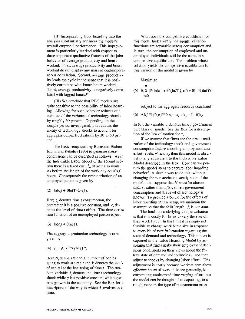
(II) Incorporating labor hoarding into theanalysis substantially enhances the model'soverall empirical performance. This improve-ment is particularly marked with respect tothree important qualitative features of the jointbehavior of average productivity and hoursworked. First, average productivity and hoursworked do not display any marked contempora-neous correlation. Second, average productiv-ity leads the cycle in the sense that it is posi-tively correlated with future hours worked.Third, average productivity is negatively corre-lated with lagged hours.1 7

(III) We conclude that RBC models arequite sensitive to the possibility of labor hoard-ing. Allowing for such behavior reduces ourestimate of the variance of technology shocksby roughly 60 percent. Depending on thesample period investigated, this reduces theability of technology shocks to account foraggregate output fluctuations by 30 to 60 per-cent.

The basic setup used by Burnside, Eichen-baum, and Rebelo (1990) to generate theseconclusions can be described as follows. As inthe Indivisible Labor Model of the second sec-tion there is a fixed cost, of going to work.As before the length of the work day equals fhours. Consequently the time t criterion of anemployed person is given by

(2) ln(c,) +

Here c, denotes time t consumption, theparameter 0 is a positive constant, and e, de-notes the level of time t effort. The time t crite-rion function of an unemployed person is just

(3) ln(c,) + Oln(T).

The aggregate production technology is nowgiven by

(4) y, = A, ktl-a(gNtetf)a.

Here N denotes the total number of bodiesgoing to work at time t and k, denotes the stockof capital at the beginning of time t. The ran-dom variable A, denotes the time t technologyshock while y is a positive constant which gov-erns growth in the economy. See the Box for adescription of the way in which A, evolves overtime.

What does the competitive equilibrium ofthis model look like? Since agents' criterionfunctions are separable across consumption andleisure, the consumption of employed and un-employed individuals will be the same in acompetitive equilibrium. The problem whosesolution yields the competitive equilibrium forthis version of the model is given by

Maximize00

(5) E0 E { ln(ct ) + 0N,ln(T-E-e,f) + 0(1-1\l i)ln(T)}t=0

subject to the aggregate resource constraint

(6) A ik,' -a(yNte rfr c, + x, +

In (6), the variable x, denotes time t governmentpurchases of goods. See the Box for a descrip-tion of the law of motion for x,.

If we assume that firms see the time t reali-zation of the technology shock and governmentconsumption before choosing employment andeffort levels, N, and e,, then this model is obser-vationally equivalent to the Indivisible LaborModel described in the Box. How can we per-turb the model so as to capture labor hoardingbehavior? A simple way to do this, withoutchanging the nonstochastic steady state of themodel, is to suppose that N, must be chosenbefore, rather than after, time t governmentconsumption and the level of technology isknown. To provide a bound for the effects oflabor hoarding in this setup, we maintain theassumption that the shift length, f, is constant.

The intuition underlying this perturbationis that it is costly for firms to vary the size oftheir work force. In the limit it is simply notfeasible to change work force size in responseto every bit of new information regarding thestate of demand and technology. This notion iscaptured in the Labor Hoarding Model by as-suming that firms make their employment deci-sions conditional on their views about the fu-ture state of demand and technology, and thenadjust to shocks by changing labor effort. Thisadjustment is costly because workers care abouteffective hours of work.1 8 More generally, in-corporating unobserved time varying effort intothe model can be thought of as capturing, in arough manner, the type of measurement error

FEDERAL RESERVE BANK OF CHICAGO 23

induced by the fact that, in many industries,reported hours worked do not vary in a one toone way with actual hours worked. This ex-planation of procyclical productivity has beenemphasized by various authors such as Fair(1969).

Suppose that an analyst computed theSolow residual using the formula S t =ytl(ktl-anta), where n, is reported hours worked at

time t. Burnside, Eichenbaum, and Rebelo(1990) show that, if labor effort is time vary-ing, the Solow residual, the stationary compo-nent of the true technology shock, and effort,are, in equilibrium, tied together via the rela-tionship

(7) S:= A t*+

Here the superscript * denotes the deviation ofthe natural log of a variable from its steadystate value. The log linear equilibrium law ofmotion for e:, the effort level, is of the form

(8)et*=plkt +psNt*+p3At*+p4gt*

where TC I 7C2'

7C3' and ; are nonlinear functions

of the structural parameters of the model.Given Burnside, Eichenbaum, and Re-

belo's point estimates of the model's structuralparameters, both it 3 and 7r4 are positive.1 9 Thisimplies that, other things equal, it is optimal towork harder when faced with a positive inno-vation in government purchases or technology,that is, effort will be procyclical. For example,Figure 2 presents the response of the LaborHoarding Model to a 1 percent innovation ingovernment consumption. By assumption, thenumber of people employed cannot immedi-ately respond to this shock. However, effortrises by over 15 percent in the first period andthen reverts to its steady state level. Panel (a)shows the implied movement in the Solowresidual. Since effort has gone up in the firstperiod but total hours of work have notchanged, the Solow residual increases by about.10 percent. This is true even though therehas been no technology shock whatsoever. Aspanel (d) shows, productivity rises in the firstperiod by .1 percent in response to the 1 per-cent innovation in government consumption.Naive Solow residual accounting falsely inter-prets the increase in average productivity asarising from a shift in technology rather thanan exogenous increase in government con-

sumption.Figure 3 shows how the Labor Hoarding

Model responds to a 1 percent innovation intechnology. Given agents' willingness to in-tertemporally substitute effective leisure overtime, they respond to the shock in the firstperiod by increasing effort by about .4 percent.As a result the Solow residual rises by 1.3percent in response to the 1 percent technologyshock. Again naive Solow residual accountingexaggerates the true magnitude of the technol-ogy shock. We conclude that naive Solowresidual accounting systematically overesti-mates the level of technology in booms, sys-tematically underestimates the level of tech-nology in recessions, and systematically over-estimates the variance of the true technologyshock.

Note that our Labor Hoarding Model doesnot allow for variations in the degree to whichcapital is utilized. The fact that capital utiliza-tion rates vary in a procyclical manner hasclear implications for the way in which move-ments in the Solow residual are interpreted.This is because the Solow residual is typicallycalculated under the assumption that the stockof capital is fully utilized. Under thesecircumstances, a change in the capital utiliza-tion rate would show up as an unexplainedincrease in output, that is, a change in theSolow residual. Since our Labor HoardingModel does not allow for time varying capitalutilization rates, it overstates thecextent towhich movements in the Solow residual arecaused by exogenous technology shocks. In-corporating capital capacity utilization deci-sions into the model would presumably furtherreduce the cyclical role of technology shocks."

Sample period sensitivity

Before discussing how incorporating laborhoarding into the model affects inferenceregarding A. we must first assess the impact ofsample period selection on inference. Numer-ous researchers have documented the fact thatthe growth rate of average productivity sloweddown substantially in the late 1960s. To docu-ment the likelihood of a break in the data, thatis, a change in the unconditional growth ofaverage productivity, Burnside, Eichebaum,and Rebelo (1990) performed a series of itera-tive Chow tests. Using these tests, we foundthat the null hypothesis of no break, that is, nochange in the unconditional growth rate, is

24 ECONOMIC PERSPECTIVES

Labor Hoarding Model—shock to government

(a) 0.20 — (b)

0.15

0.10

0.2

0.1

Measured APL(Average productivity

of labor)

0.0

-0.10

FIGURE 2

rejected at very high significance levels at alldates during the interval 1966:1-1974:2. Theactual break point we chose was 1969:4, how-ever, our results are not sensitive to the precisebreak point used.

In the same article we also discuss theimpact of allowing for a break in the data onour estimates of the structural parameters. Forboth the Indivisible Labor Model and the La-bor Hoarding Model, there are four importantdifferences in the parameter values across thedifferent sample periods. First, the estimatedvalues of the unconditional growth rate of theSolow residual, in the first and second sampleperiods, .0069 and .0015 respectively, arequite different. Second, the estimated value ofthe coefficient governing serial correlation inthe technology shock, p,, is quite sensitive to abreak in the sample period. For example,using the Indivisible Labor Model, the esti-mated value of pa over the whole period

(.986), is substantially larger than those ob-tained in the first (.86) and second (.88)sample periods. This is exactly what wewould expect if there were indeed a break inthe Solow residual process...2 1 Third, estimatesof G, the standard error of the innovation totechnology, are also quite sensitive to thechoice of sample period. The estimated valueof oE equals .0060, .0101, and .0089, in thefirst, second, and whole sample periods, re-spectively. Fourth, the estimates of 7, (thegrowth rate in government consumption), p g

(the parameter which governs serial correla-tion in government purchases), and o l, (thestandard error of the innovation to governmentpurchases) are affected in the same qualitativeway as the analog parameters governing theevolution of the Solow residual. However thequantitative differences are even larger.

These results have an important impact onthe models' implications for some of standard

FEDERAL RESERVE BANK OF CHICAGO 25

•• MeasUred'API ..(measured prodtictlyity,.... ,

0( labor) •.: ••:.: ,••:• •

Labor Hoarding Model—shock to technology

(a) 1.6 -

Solow residual

diagnostic moments discussed in the secondsection. Table 3 reports the Labor Hoardingand Indivisible Labor Models' predictions forcs, 6/6„ 016„ 6416,, and oi/ APL over thewhole sample period. In addition that table re-ports our estimates of the corresponding datamoments. Table 4 reports the correspondingresults for the two subsample periods. Takentogether, these tables substantiate our claimthat the empirical performance of RBC modelsdepends on sample period selection.

Recall that when the Indivisible LaborModel was estimated over the whole sampleperiod, there was very little evidence againstthe model's implications for these moments.Table 3 shows that this is also true for theLabor Hoarding Model. Using the wholesample there is very little evidence against theindividual hypotheses that the values of6", Gt lo v' 6 rlo or 6 4/6, that emergefrom either model are different from the corre-

sponding data population moments. However,Table 4 indicates that the performance of bothmodels deteriorates significantly when weallow for a break in the sample. This deterio-ration is quite pronounced with respect to therelative volatility of consumption and invest-ment. Indeed using either sample period, andany conventional significance level, we canreject the hypotheses that these model mo-ments equal the corresponding data populationmoments. Interestingly this result is not due tothe fact that the data moment estimates changesubstantially. Rather, it is due to the fact thatthe models' implications for the two momentsappear to be quite sensitive to a break in thesample. For example over the whole sampleperiod, both models imply that consumption isroughly half as volatile as output. However,when estimated on the separate sample peri-ods, both models predict that consumption is

26 ECONOMIC PERSPECTIVES

TABLE :3

Indivisible Labor Model vs. LaborHoarding Model—selected

second moments

Whole sample*

Second U.S.moment data**

ajcs, .44(.03)

cs/cs, 2.22(.07)

allay 1.15(.20)

C5n/GAPL 1.22(.12)

an .017(.002)

IndivisibleLabor

Model***

.53(.24)[.69]

2.65(.59)[.47]

1.09(.35)[.89]

1.053(.46)[.721

.013(.005)[.94]

LaborHoarding

Model

.48(.19)[.80]

2.77(.45)[.23]

1.29(.15)[.50]

1.017(.41)[.39]

.013(.003)[.76]

SOURCE: C. Burnside, M. Eichenbaum, and S. Rebelo,"Labor hoarding and the business cycle," manuscript,Northwestern. University."Whole sample corresponds to the sample period

1955:3-1984:4.**Numbers in parentheses correspond to standarderrors.***Numbers in brackets refer to the probability valueof the test statistic used by Burnside, Eichenbaum, andRebelo (1990) to test whether a model and data mo-ment are the same in population.

only a fourth as volatile as output.The intuition behind this last result is

straightforward. According to the permanentincome hypothesis, an innovation to laborincome causes households to revise their con-sumption by an amount equal to the annuityvalue of that innovation. If income was a firstorder autoregressive process that displayedpositive serial correlation, then the annuityvalue of the innovation would be a strictlyincreasing function of the coefficient govern-ing serial correlation in income. Using amodel very similar to our Indivisible LaborModel, Christiano (1987) shows that the in-come effect of an innovation to the technologyshock depends positively on the value of p a ,the parameter which governs the serial correla-tion of the technology shock. Since the pointestimate of p a falls in both subsamples, we

would expect that, holding interest rates con-stant, the response of consumption to an inno-vation in the technology shock should also fall.Given that Christiano (1987) also shows thatthe impact of technology shocks on the interestrate in standard RBC models is quite small, itis not surprising that the model predicts lowervalues for o /a in the subsample periods.Since output equals consumption plus invest-ment plus government consumption, and thelatter does not respond to technology shocks, itfollows that, other things equal, investment ismore volatile because consumption is lessvolatile.

Labor hoarding and X

Given the sensitivity of inference tosample period selection, we allow for a breakin the data in reporting the impact of laborhoarding on A.. To begin with, consider theimplications of allowing for time varyingeffort on the parameters governing the law ofmotion of technology shocks. ComparingTables 5 and 6 we see that this change in themodel leads to a large reduction in 6 E . Basedon the whole sample period, the variance(square of the standard error reported in thetable) of the innovation to technology shocksdrops by roughly 35 percent. In Sample period1 and Sample period 2 this variance drops by48 and 56 percent, respectively. Evidently,breaking the sample magnifies the sensitivityof estimates of oE to time varying effort. Adifferent way to assess this sensitivity is toconsider the unconditional variance of thestationary component of the technology shock,

, which equals oE/(1–pa2). Allowing for timevarying effort reduces the volatility of technol-ogy shocks by over 58 percent in the wholesample period, 49 percent in Sample period 1,and 57 percent in Sample period 2. Theseresults provide support for the view that alarge percentage of the movements in theobserved Solow residual may be artifacts oflabor hoarding type behavior.

How do these findings translate intochanges regarding the model's implications fork? Tables 5 and 6 indicate that over the wholesample period, introducing labor hoarding intothe analysis causes 2 to decline by 28 percentfrom .81 to .58. The sensitivity of X is evenmore dramatic once we allow for a break inthe sample. Labor hoarding reduces X by 58percent in the first sample period and by 63

FEDERAL RESERVE BANK OF CHICAGO

27

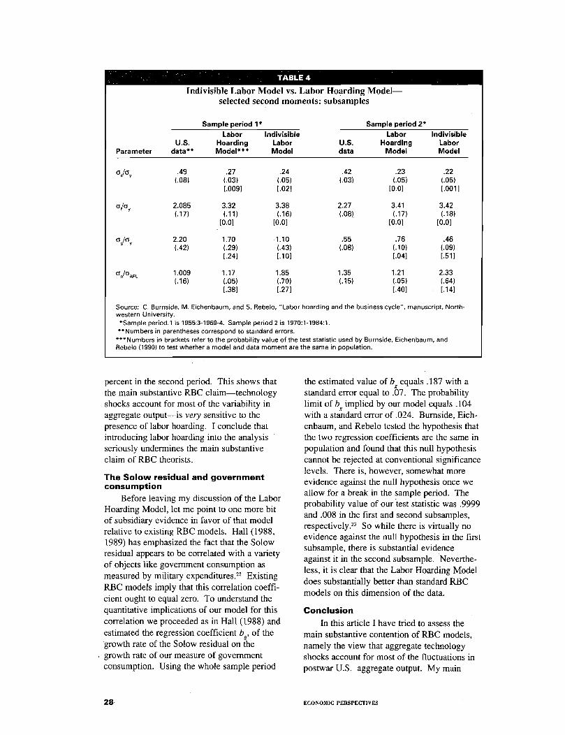
TABLE 4

Indivisible Labor Model vs. Labor Hoarding Model-selected second moments: subsamples

Sample period 1* Sample period 2*

Labor

Indivisible

Labor

IndivisibleU.S. Hoarding

Labor

U.S. Hoarding

LaborParameter data**

Model***

Model

data

Model

Modelon/oAPL

oc/oy .49(.08)

.27(.03)[.0091

.24 .42(.05) (.03)[.021

.23 .22

(.05) (.05)

[0.0] [.001]

oloy 2.085(.17)

3.32(.11)

[0.0]

3.38(.16)

[0.0]

2.27(.08)

3.41 3.42(.17) (.18)

[0.0] [0.0]og/oy

2.20(.42)

1.70(.29)[.24]

1.10 .55(.43) (.08)[.10]

.76 .46(.10) (.09)[.04] [.51]

1.009 1.17

1.85

1.35

1.21 2.33(.16) (.05)

(.70)

(.15)

(.05) (.64)[.38]

[.27]

[.40] [.14]

Source: C. Burnside, M. Eichenbaum, and S. Rebelo, "Labor hoarding and the business cycle", manuscript, North-western University.*Sample period .1 is 1955:3-1969-4. Sample period 2 is 1970:1-1984:1.**Numbers in parentheses correspond to standard errors.***Numbers in brackets refer to the probability value of the test statistic used by Burnside, Eichenbaum, andRebelo (1990) to test whether a model and data moment are the same in population.

percent in the second period. This shows thatthe main substantive RBC claim-technologyshocks account for most of the variability inaggregate output-is very sensitive to thepresence of labor hoarding. I conclude thatintroducing labor hoarding into the analysisseriously undermines the main substantiveclaim of RBC theorists.

The Solow residual and governmentconsumption

Before leaving my discussion of the LaborHoarding Model, let me point to one more bitof subsidiary evidence in favor of that modelrelative to existing RBC models. Hall (1988,1989) has emphasized the fact that the Solowresidual appears to be correlated with a varietyof objects like government consumption asmeasured by military expenditures. 22 ExistingRBC models imply that this correlation coeffi-cient ought to equal zero. To understand thequantitative implications of our model for thiscorrelation we proceeded as in Hall (1988) andestimated the regression coefficient b, of thegrowth rate of the Solow residual on thegrowth rate of our measure of governmentconsumption. Using the whole sample period

the estimated value of b equals .187 with astandard error equal to .07. The probabilitylimit of b implied by our model equals .104with a standard error of .024. Burnside, Eich-enbaum, and Rebelo tested the hypothesis thatthe two regression coefficients are the same inpopulation and found that this null hypothesiscannot be rejected at conventional significancelevels. There is, however, somewhat moreevidence against the null hypothesis once weallow for a break in the sample period. Theprobability value of our test statistic was .9999and .008 in the first and second subsamples,respectively. 23 So while there is virtually noevidence against the null hypothesis in the firstsubsample, there is substantial evidenceagainst it in the second subsample. Neverthe-less, it is clear that the Labor Hoarding Modeldoes substantially better than standard RBCmodels on this dimension of the data.

Conclusion

In this article I have tried to assess themain substantive contention of RBC models,namely the view that aggregate technologyshocks account for most of the fluctuations inpostwar U.S. aggregate output. My main

28

ECONOMIC PERSPECTIVES

TABLE 5 TABLE 6

Indivisible Labor Model-variability of output: subsamples

P.

Labor Hoarding Model-variability of output: subsamples

r 6Ym

Whole sample* .0089 .986 .017 .81 Whole sample* .0072 .977 .015 .58(.0013) (.026) (.6) (.56) (.0012) (.029) (.001) (.14)

Sample period 1* .0060 .862 .017 1.69 Sample period 1* .0042 .869 .011 .71(.0022) (.071) (.7) (1.51) (.0006) (.043) (.001) (.20)

Sample period 2* .0101 .884 .028 1.42 Sample period 2* .0067 .882 .017 .52(.0015) (.065) (.005) (.65) (.0006) (.061) (.001) (.12)

SOURCE: C. Burnside, M. Eichenbaum, and S. Rebelo,"Labor hoarding and the business cycle," manuscript,Northwestern University.*Whole sample corresponds to the sample period 1955:3-1984:4. Sample period 1 is 1955:3-1969:4. Sample period2 is 1970:1-1984:1.**Numbers in parentheses correspond to standard errors.

conclusion is that the evidence presented byRBC analysts is too fragile to justify thisstrong claim. It does not seriously underminethe traditional view that shocks to aggregatedemand are the key source of impulses to thebusiness cycle.

However, the RBC literature has suc-ceeded in showing that dynamic stochasticgeneral equilibrium models can be used tosuccessfully organize our thoughts about thebusiness cycle in a quantitative way. Onecannot help but be impressed by the ability ofsimple RBC models to reproduce certain key

SOURCE: C. Burnside, M. Eichenbaum, and S. Rebelo,"Labor hoarding and the business cycle," manuscript,Northwestern University.*Whole sample corresponds to the sample period 1955:3-1984:4. Sample period 1 is 1955:3-1969:4. Sample period2 is 1970:1-1984:1.**Numbers in parentheses correspond to standard errors.

moments of the data. In my view, too muchprogress has been made to revert to the nihil-ism of purely statistical analyses of the data.Certainly we need to know the facts. Butdesigning good policy requires more thanatheoretic summaries of the data. Good policydesign requires empirically plausible structuraleconomic models. The achievements of theRBC literature reinforce my optimism thatprogress is possible. The failures of that litera-ture reinforce my view that we have some wayto go before we can declare success.

FOOTNOTES

'See, for example, Summers (1986).

2. This is not quite correct in a general equilibrium context.If consumers/labor suppliers own the goods producingfirms, then there is also an income effect associated with atechnology shock. If leisure is a normal good, then, otherthings equal, the labor supply curve would shift inwards inresponse to a positive technology shock. Christiano andEichenbaum (1990) show that when a technology shock isnot permanent the quantitative impact of this effect isnegligible.

3See Aiyagari, Christiano, and Eichenbaum (1990) for adiscussion of the effects of government purchases in thestochastic one sector growth model.

4See, for example, Kydland and Prescott (1982, 1989).

5See, for example, Hansen (1988).

6See Christiano and Eichenbaum (forthcoming).

7See, for example, Prescott (1986).

8 See, for example, Kydland and Prescott (1982), Hansen(1985), Prescott (1986), Kydland and Prescott (1988), andBackus, Kehoe,and Kydland (1989).

9See King and Rebelo (1988). Also, in recent, workKuttner (1990) has shown that the cyclical component ofHP filtered data resembles one concept of potential realGNP quite closely.

10 Our point estimates of a, 0, 8, pa , oE, pg, and a l, equal.655 (.006), 3.70 (.040), .021 (.0003), .986 (.026), .0089(.0013), .979 (.021), and .0145 (.0011). See Bumside,Eichenbaum, and Rebelo (1990) for details.

"The data and econometric methodology underlying theseestimates are discussed in Burnside, Eichenbaum, and

FEDERAL RESERVE BANK OF CHICAGO 29

Rebelo (1990). Our point estimates of a, 0, 5, p., and a.,equal .655 (.006), 3.70 (.040), .021 (.0003), .986 (.026),

and .0089 (.0013). Numbers in parentheses denote stan-dard errors.

12 See Hansen (1988) and Christiano and Eichenbaum(1990).

13 Including government in the model does have important

implications for the model's predictions along other dimen-

sions of the data such as the correlation between averageproductivity and hours worked. See Christiano and Eichen-

baum (forthcoming).

14 Our point estimate of d is .019 with standard error of

.002.

15 See Burnside, Eichenbaum, and Rebelo (1990).

16 The method used by Burnside, Eichenbaum, and Rebelo

(1990) to estimate the model's structural parameters

amounts to an exactly identified version of Hansen's(1982) Generalized Method of Moments procedure. Pre-

sumably the confidence interval could be narrowed byimposing more of the model's restrictions, say via a maxi-

mum likelihood estimation procedure or an over-identifiedGeneralized Method of Moments procedure. Using such

procedures would result in substantially different estimatesof making comparisons with the existing RBC literaturevery difficult. See Christiano and Eichenbaum (forthcom-

ing) for a discussion of this point.

"Gordon (1979) presents evidence on this general phe-

nomenon which he labels the "end-of-expansion-productiv-ity-slowdown". McCallum (1989) also documents a similarpattern for the dynamic correlations between average

productivity and output.

"It follows that labor must be compensated for workingharder. We need not be precise about the exact compensa-tion scheme because the optimal decentralized allocationcan be found by solving the appropriate social planningproblem for our model economy.

19 For this model our point estimates of a, 0, 5, p., oE, p g ,

and 6 equal .655 (.006), 3.68 (.033), .021 (.0003), .977

(.029), .0072 (.0012), .979 (.021), and .0145 (.0011). SeeBurnside, Eichenbaum, and Rebelo (1990) for details.

201n ongoing research Craig Burnside and I are investigat-

ing this issue.

21 See Perron (1988).

22 Hall (1989) argues that time varying effort is not a plau-

sible explanation of this correlation. To show this, he first

calculates the growth rate of effective labor input requiredto explain all of the observed movements in total factor

productivity. From this measure he subtracts the growth

rate of actual hours work to generate a time series on thegrowth rate in work effort. He argues that the implied

movements in work effort are implausibly large. Thiscalculation does not apply to our analysis because it pre-

sumes that there are no shocks to productivity, an assump-

tion which is clearly at variance with our model.

231n the first sample the point estimate of N5 is .0798 withstandard error .0795. The value of N5 that emerges fromour model is .0797 with a standard error of .0259. For the

second sample the point estimate Of N o is .280 with a stan-dard error of .099, while the value of N implied by the

model is .0225 with a standard error o1.004.

REFERENCES

Aiyagari, S. Rao, Lawrence J. Christiano,and Martin Eichenbaum, "The output, em-ployment, and interest rate effects of govern-ment consumption," Working Paper Series,Macro Economic Issues, Research Depart-ment, Federal Reserve Bank of Chicago, WP-90-91, 1990 .

Backus, David K., Patrick J. Kehoe, andFinn E. Kydland, "International trade andbusiness cycles," Federal Reserve Bank ofMinneapolis, Working Paper 425, 1989.

Blanchard, Olivier J., "A traditional interpre-tation of macroeconomic fluctuations," Ameri-can Economic Review, 79, 1989, pp. 1146-1164.

Burnside, Craig, Martin Eichenbaum, andSergio T. Rebelo, "Labor hoarding and the

business cycle," Manuscript, NorthwesternUniversity, 1990.

Christiano, Lawrence J., "Why is consump-tion less volatile than income?" Federal Re-serve Bank of Minneapolis, Quarterly Review,1, 1987, pp. 2-20.

Christiano, Lawrence J., and Martin Eich-enbaum, "Unit roots in real GNP—Do weknow and do we care?," Carnegie-RochesterConference Series on Public Policy: UnitRoots, Investment Measures and Other Essays,Allan H. Meltzer, ed., 32, 1990, pp. 7-62.

Christiano, Lawrence J., and Martin Eich-enbaum, "Current real business cycle theoriesand aggregate labor market fluctuations,"American Economic Review, forthcoming.

30 ECONOMIC PERSPECTIVES

Evans, Charles L., "Productivity shocks andreal business cycles," Manuscript, Universityof South Carolina, 1990.

Kydland, Finn E., and Edward C. Prescott,"The work week of capital and its cyclicalimplications," Journal of Monetary Econom-ics, 21, 1988, pp. 343-60.

Fair, Ray, The Short Run Demand for Work-ers and Hours, North-Holland PublishingCompany: Amsterdam, 1969.

Gordon, Robert J., "The end-of-expansionphenomenon in short-run productivity behav-ior," Brookings Papers on Economic Activity,2, 1979, pp. 447-61.

Hall, Robert E., "The relation between priceand marginal cost in U.S. industry," Journal ofPolitical Economy, 96, 1988, pp. 921-47.

Hall, Robert E., "Invariance properties of theSolow residual," The NBER, Working Paper3034, 1989.

Hansen, Gary D., "Indivisible labor and thebusiness cycle," Journal of Monetary Eco-nomics, 16, 1985, pp. 309-28.

Hansen; Gary D., "Technical progress andaggregate fluctuations," Manuscript, Univer-sity of California, Los Angeles, 1988.

Hansen, Lars P., "Large sample properties ofgeneralized method of moments estimators,"Econometrica, 50, 1982, pp. 1029-54.

Hodrick, Robert J., and Edward C.Prescott, "Post-war U.S. business cycles: anempirical investigation," Manuscript, Carne-gie-Mellon University, 1980.

King, Robert G., and Sergio T. Rebelo,"Low frequency filtering and real businesscycles," Manuscript, University of Rochester,1988.

Kuttner, Kenneth., "A new approach to non-inflationary potential GNP," manuscript, Fed-eral Reserve Bank of Chicago, 1990.

Kydland, Finn E., and Edward C. Prescott,"Time to build and aggregate fluctuations,"Econometrica, 50, 1982, pp. 1345-70.

Kydland, Finn E., and Edward C. Prescott,"Hours and employment variation in businesscycle theory," Institute for Empirical Econom-ics, Discussion Paper 17, 1989.

Lucas, Robert E. Jr., "Capacity, overtime,and empirical production functions," AmericanEconomic Review, Papers and Proceedings, 6,1970, pp. 1345-1371.

Lucas, Robert E. Jr., "Expectations and theneutrality of money," Journal of EconomicTheory, 4, 1972, pp. 103-124.

Lucas, Robert E. Jr., "The effects of mone-tary shocks when prices are set in advance,"Manuscript, University of Chicago, November,1989.

McCallum, Bennett T., "Real business cyclemodels," Modern Business Cycle Theory,Robert J. Barro, ed., Harvard University Press,1989, pp. 16-50.

Perron, P., "The great crash, the oil priceshock, and the unit root hypothesis," Econom-etrica, 55, 1988, pp. 277-302.

Prescott, Edward C., "Theory ahead of busi-ness cycle measurement," Federal ReserveBank of Minneapolis, Quarterly Review, 10,1986, pp. 9-22.

Rogerson, R., "Indivisible labor, lotteries andequilibrium," Journal of Monetary Economics,21, 1988, pp. 3-17.

Summers, Lawrence J., "Some skepticalobservations on real business cycle theory,"Federal Reserve Bank of Minneapolis, Quar-terly Review, 10, 1986, pp. 23-27.

FEDERAL RESERVE BANK OF CHICAGO 31