HITCHIN INTEGRABLE SYSTEMS, DEFORMATIONS OF SPECTRAL ...mulase/texfiles/spectral2008.pdf · HITCHIN...
35
HITCHIN INTEGRABLE SYSTEMS, DEFORMATIONS OF SPECTRAL CURVES, AND KP-TYPE EQUATIONS ANDREW R. HODGE 1 AND MOTOHICO MULASE 2 Abstract. An effective family of spectral curves appearing in Hitchin fibra- tions is determined. Using this family the moduli spaces of stable Higgs bun- dles on an algebraic curve are embedded into the Sato Grassmannian. We show that the Hitchin integrable system, the natural algebraically completely inte- grable Hamiltonian system defined on the Higgs moduli space, coincides with the KP equations. It is shown that the Serre duality on these moduli spaces corresponds to the formal adjoint of pseudo-differential operators acting on the Grassmannian. From this fact we then identify the Hitchin integrable system on the moduli space of Sp 2m -Higgs bundles in terms of a reduction of the KP equations. We also show that the dual Abelian fibration (the SYZ mirror dual) to the Sp 2m -Higgs moduli space is constructed by taking the symplectic quotient of a Lie algebra action on the moduli space of GL-Higgs bundles. 1. Introduction The purpose of this paper is to determine the relation between the KP-type equations defined on the Sato Grassmannians and the Hitchin integrable systems defined on the moduli spaces of stable Higgs bundles. The results established are the following: (1) We determine the effective family of spectral curves appearing in the Hitchin fibration of the moduli spaces of stable Higgs bundles. (2) We embed the effective family of Jacobian varieties of the spectral curves into the Sato Grassmannian and show that the KP flows are tangent to each fiber of the Hitchin fibration. (3) The moduli space of Higgs bundles of rank n and degree n(g - 1) on an algebraic curve of genus g ≥ 2 is embedded into the relative Grassmannian of [2, 4, 23]. Using this embedding we show that the Hitchin integrable system is exactly the restriction of the KP equations on the Grassmannian to the image of this embedding. (4) It is shown that the Krichever construction transforms the Serre duality of the geometric data consisting of algebraic curves and vector bundles on them to the formal adjoint of pseudo-differential operators acting on the Grassmannian. By identifying the fixed-point-set of the Serre duality and the formal adjoint operation we determine the KP-type equations that are 2000 Mathematics Subject Classification. 14H60, 14H70, 35Q53, 37J35. Key words and phrases. Hitchin Integrable System, Spectral Curve, Higgs Bundle, Sato Grass- mannian, Symplectic KP Equation. 1 Research supported by NSF grants DMS-0135345 (VIGRE) and DMS-0406077 while at UC Davis. 2 Research supported by NSF grant DMS-0406077 and UC Davis. 1
Transcript of HITCHIN INTEGRABLE SYSTEMS, DEFORMATIONS OF SPECTRAL ...mulase/texfiles/spectral2008.pdf · HITCHIN...
HITCHIN INTEGRABLE SYSTEMS, DEFORMATIONS OFSPECTRAL CURVES, AND KP-TYPE EQUATIONS
ANDREW R. HODGE1 AND MOTOHICO MULASE2
Abstract. An effective family of spectral curves appearing in Hitchin fibra-
tions is determined. Using this family the moduli spaces of stable Higgs bun-dles on an algebraic curve are embedded into the Sato Grassmannian. We show
that the Hitchin integrable system, the natural algebraically completely inte-
grable Hamiltonian system defined on the Higgs moduli space, coincides withthe KP equations. It is shown that the Serre duality on these moduli spaces
corresponds to the formal adjoint of pseudo-differential operators acting on the
Grassmannian. From this fact we then identify the Hitchin integrable systemon the moduli space of Sp2m-Higgs bundles in terms of a reduction of the
KP equations. We also show that the dual Abelian fibration (the SYZ mirror
dual) to the Sp2m-Higgs moduli space is constructed by taking the symplecticquotient of a Lie algebra action on the moduli space of GL-Higgs bundles.
1. Introduction
The purpose of this paper is to determine the relation between the KP-typeequations defined on the Sato Grassmannians and the Hitchin integrable systemsdefined on the moduli spaces of stable Higgs bundles. The results established arethe following:
(1) We determine the effective family of spectral curves appearing in the Hitchinfibration of the moduli spaces of stable Higgs bundles.
(2) We embed the effective family of Jacobian varieties of the spectral curvesinto the Sato Grassmannian and show that the KP flows are tangent toeach fiber of the Hitchin fibration.
(3) The moduli space of Higgs bundles of rank n and degree n(g − 1) on analgebraic curve of genus g ≥ 2 is embedded into the relative Grassmannianof [2, 4, 23]. Using this embedding we show that the Hitchin integrablesystem is exactly the restriction of the KP equations on the Grassmannianto the image of this embedding.
(4) It is shown that the Krichever construction transforms the Serre dualityof the geometric data consisting of algebraic curves and vector bundles onthem to the formal adjoint of pseudo-differential operators acting on theGrassmannian. By identifying the fixed-point-set of the Serre duality andthe formal adjoint operation we determine the KP-type equations that are
2000 Mathematics Subject Classification. 14H60, 14H70, 35Q53, 37J35.Key words and phrases. Hitchin Integrable System, Spectral Curve, Higgs Bundle, Sato Grass-
mannian, Symplectic KP Equation.1Research supported by NSF grants DMS-0135345 (VIGRE) and DMS-0406077 while at UC
Davis.2Research supported by NSF grant DMS-0406077 and UC Davis.
1

2 ANDREW HODGE AND MOTOHICO MULASE
equivalent to the Hitchin integrable system defined on the moduli space ofSp2m-Higgs bundles.
(5) There are two ways to reduce an algebraically completely integrable Hamil-tonian system: one by restriction and the other by taking a quotient of a Liealgebra action that is similar to the symplectic quotient. When applied tothe moduli spaces of Higgs bundles, these constructions yield SYZ-mirrorpairs. We interpret the SL-PGL and Sp2m-SO2m+1 dualities in this way.
Let GC be the category of complex Lie groups, and CY the category of Calabi-Yauspaces. For a compact oriented surface Σ of genus g ≥ 2, the functor
Hom(π1(Σ), · )// · : GC −→ CYassigns to each complex Lie group G its character variety
Hom(π1(Σ), G
)//G,
where π1(Σ) is the central extension of the fundamental group of Σ. The quotientby conjugation is the geometric invariant theory quotient of Mumford [21]. Anamazing discovery of Hausel and Thaddeus [8], and its generalizations by [5, 14]and others, is that the character variety functor transforms the Langlands dualityin GC to the mirror symmetry of Calabi-Yau spaces in the sense of Strominger-Yau-Zaslow [28]:
GCHom(π1(Σ), · )// ·−−−−−−−−−−−−→ CY
Langlands Dual
y yMirror Dual
GC −−−−−−−−−−−−→Hom(π1(Σ), · )// ·
CY
The character variety Hom(π1(Σ), G
)//G has many distinct complex structures [8,
14]. To understand the SYZ mirror symmetry among the character varieties, it ismost convenient to realize them as Hitchin integrable systems. In his seminal papers[10, 11], Hitchin identifies the character variety with the moduli space of stableG-Higgs bundles, which has the structure of an algebraically completely integrableHamiltonian system.
An algebraically completely integrable Hamiltonian system [4, 31] is a holomor-phic symplectic manifold (X,ω) of dimension 2N together with a holomorphic mapH : X → g∗ such that
(1) a general fiber H−1(s), s ∈ g∗, is an Abelian variety of dimension N ,(2) g∗ is the dual Lie algebra of a general fiber H−1(s) considered as a Lie
group, and(3) the coordinate components of the map H are Poisson commutative with
respect to the symplectic structure ω.The notion corresponding to an algebraically completely integrable Hamiltonian
system in real symplectic geometry is the cotangent bundle of a torus. The proce-dure of symplectic quotient is to remove the effect of this cotangent bundle from agiven symplectic manifold. In the holomorphic context, it is often useful to take thequotient by a family of groups that have the same Lie algebra. Suppose we have aLie algebra direct sum decomposition g = g1⊕g2. If g1-action on X is integrable toa group G1,s-action in each fiber H−1(s) for s ∈ g∗2, then we can define a quotientX//g1 as the family of quotients H−1(s)/G1,s over g∗2. We can also construct a re-duction of (X,ω,H) by restricting the fibration to g∗2 and considering the family of
HITCHIN SYSTEMS, SPECTRAL CURVES, AND KP EQUATIONS 3
g2-orbits in H−1(s), if the g2-action is integrated to a group action over g∗2. Whenapplied to the moduli space of Higgs bundles, these two constructions yield Abelianfibrations that are dual to one another, producing an SYZ mirror pair. We examinethese constructions for the SL-PGL and Sp2m-SO2m+1 dualities.
From the results established in [4, 16, 17, 19], we know that linear integrableevolution equations on the Jacobians or Prym varieties are realized as the restrictionof KP-type equations defined on the Sato Grassmannians through a generalizationof Krichever construction. Since the Hitchin integrable systems are defined on afamily of Jacobian varieties or Prym varieties, we need to embed the whole familyinto the Sato Grassmannian to compare the Hitchin systems and the KP equations.To deal with families, we use two different approaches in this article. One approachis to utilize the theory of Sato Grassmannians defined over an arbitrary schemedeveloped in [2, 4, 22, 23]. In this way we can directly compare the integrableHamiltonian systems on the Higgs moduli spaces and the KP equations. The otherapproach is to examine the deformations of spectral curves that appear in theHitchin Hamiltonian systems. Once we identify the effective family of spectralcurves, we can embed the whole family into a single Sato Grassmannian over C,using the method developed in [16].
The second approach has an unexpected application: we can identify the effectof Serre duality operation on the algebro-geometric data in terms of the languageof Grassmannians. Note that Sato Grassmannians are constructed from pseudo-differential operators [24, 25]. We will show, using Abel’s theorem, that the Serreduality is simply the formal adjoint operation on the pseudo-differential operators.Since the Sp-Hitchin system is the fixed-point-set of the Serre duality on the GL-Hitchin system, we can determine the integrable equations corresponding to the Spcase as a reduction of the KP equations on the fixed-point-set of the formal adjointaction on pseudo-differential operators. Since our formal adjoint is slightly differentfrom what has been studied in the literature [13, 27, 29], the equations coming upfor the symplectic groups are not BKP or CKP equations. Let
P =∑
ai(x)(∂
∂x
)ibe a formal pseudo-differential operator, where ai(x) is a matrix valued functions.We define the formal adjoint by
P ∗ =∑(
∂
∂x
)i· ai(−x)t.
The reduction of the KP equations that corresponds to the Sp-Hitchin system isthe 2m-component KP equations that preserve the algebraic condition
(1.1) L∗ =[
ImIm
]· L ·
[Im
Im
]for a 2m × 2m matrix Lax operator L with the leading term I2m · ∂/∂x. Severalauthors have proposed integrable systems with Sp2m-symmetry (cf. [30]). It wouldbe interesting to study our reduction (1.1) from the point of view of integrablesystems and to investigate the relation with the other Sp integrable systems.
The fundamental literature of the algebro-geometric study of the Hitchin inte-grable systems and related topics is the book [4] by Donagi and Markman. Our

4 ANDREW HODGE AND MOTOHICO MULASE
present paper employs a slightly different perspective, that leads to the discoveryof the KP-type equations corresponding to the Sp Hitchin system.
The relation between the Hitchin integrable systems and the KP equations wasalso studied in [15]. The treatment there was limited to the study of the Hitchinsystem on a single fiber. The present article extends the result therein.
We also note that many topics of this paper have been studied by the Salamancaschool of algebraic geometers from yet another point of view [2, 7, 9, 22].
The paper is organized as follows. The first section is devoted to reviewingthe Hitchin integrable systems of [3, 11]. We then determine an effective familyof spectral curves in Section 3. Section 4 is devoted to giving two constructionsof reduced integrable systems from a Hitchin system: one is a straightforwardspecialization, and the other is a kind of symplectic reduction by a Lie subalgebra.These two constructions give rise to an Abelian fibration and its dual Abelianfibration. We show that the GL-Hitchin integrable system is equivalent to theKP equations in Section 5. The identification of the Serre duality in terms ofGrassmannians and pseudo-differential operators is carried out in Section 6. Finallywe determine the KP-type equations for the Sp Hitchin system.
2. Hitchin integrable systems
In this section we review the algebraically completely integrable Hamiltoniansystems defined on the moduli spaces of Higgs bundles, following [3, 4, 10, 11].
Throughout the paper we denote by C a non-singular algebraic curve of genusg ≥ 2. The moduli space of semistable algebraic vector bundles on C of rank n anddegree d is denoted by UC(n, d). When n and d are relatively prime, a semistablebundle is automatically stable, and the moduli space is a non-singular projectivealgebraic variety of dimension n2(g − 1) + 1. We denote by
(2.1) UC(n) =∐d∈ZUC(n, d)
the space of all stable vector bundles. A Higgs bundle is a pair (E, φ) consisting ofan algebraic vector bundle E on C and a global section
(2.2) φ ∈ H0(C,End(E)⊗KC)
of the endomorphism sheaf of E twisted by the canonical sheaf KC of C. A Higgsbundle is stable if degF
rankF < degErankE for every φ-invariant proper holomorphic vector
subbundle F . An endomorphism of a Higgs bundle (E, φ) is an endomorphism ψof E that commutes with φ:
Eψ−−−−→ E
φ
y yφE ⊗KC −−−−→
ψ⊗1E ⊗KC
It is known that H0(C,End(E, φ)) = C for a stable Higgs bundle, and one candefine the moduli space of stable objects. We denote by HC(n, d) the moduli spaceof stable Higgs bundles of rank n and degree d on C, and
(2.3) HC(n) =∐d∈ZHC(n, d).

HITCHIN SYSTEMS, SPECTRAL CURVES, AND KP EQUATIONS 5
Note that the Serre duality induces an involution on HC(n) defined by
(2.4) HC(n, d) 3 (E, φ) 7−→ (E∗ ⊗KC ,−φ∗) ∈ HC(n,−d+ 2n(g − 1)).
The dual of the Higgs field φ : E → E ⊗KC is a homomorphism φ∗ : E∗ ⊗K−1C →
E∗. We use the same notation for the homomorphism E∗ ⊗ KC → E∗ ⊗ K⊗2C
induced by φ∗.If E is stable, then (E, φ) is stable for any φ of (2.2). And if φ = 0, then the
stability of (E, φ) simply means E is stable. Therefore, the Higgs moduli spacecontains the total space of the holomorphic cotangent bundle
(2.5) T ∗UC(n, d) ⊂ HC(n, d),
sinceH0(C,End(E)⊗KC) ∼= H1(C,End(E))∗ ∼= T ∗E UC(n, d).
Note that p∗Λ1(UC(n, d)) ⊂ Λ1(T ∗UC(n, d)) has a tautological section
(2.6) η ∈ H0(T ∗UC(n, d), p∗Λ1(UC(n, d))),
where p : T ∗UC(n, d) → UC(n, d) is the projection, and Λr denotes the sheaf ofholomorphic r-forms. The differential ω = −dη of the tautological section definesthe canonical holomorphic symplectic form on T ∗UC(n, d). The restriction of ω onUC(n, d), which is the 0-section of the cotangent bundle, is identically 0. Thereforethe 0-section is a Lagrangian submanifold of this holomorphic symplectic space.
Let us denote by
(2.7) V ∗GL = V ∗GLn(C) =n⊕i=1
H0(C,K⊗iC ).
As a vector space V ∗GL has the same dimension of H0(C,End(E)⊗KC). The Higgsfield φ : E → E ⊗KC induces a homomorphism of the i-th anti-symmetric tensorproduct spaces
∧i(φ) : ∧i(E) −→ ∧i(E ⊗KC) = ∧i(E)⊗K⊗iC ,
or equivalently ∧i(φ) ∈ H0(C,End(∧i(E)) ⊗ K⊗iC ). Taking its natural trace, weobtain
tr ∧i (φ) ∈ H0(C,K⊗iC ).
This is exactly the i-th characteristic coefficient of the twisted endomorphism φ:
(2.8) det(x− φ) = xn +n∑i=1
(−1)itr ∧i (φ) · xn−i.
By assigning the coefficients of (2.8), Hitchin [11] defines a holomorphic map, nowknown as the Hitchin fibration or Hitchin map,
(2.9) H : HC(n, d) 3 (E, φ) 7−→ det(x− φ) ∈n⊕i=1
H0(C,K⊗iC ) = V ∗GL.
The map H to the vector space V ∗GL is a collection of N = n2(g − 1) + 1 globallydefined holomorphic functions on HC(n, d). The 0-fiber of the Hitchin fibration isthe moduli space UC(n, d).

6 ANDREW HODGE AND MOTOHICO MULASE
To determine the generic fiber of H, the notion of spectral curves is introducedin [11]. The total space of the canonical sheaf KC = Λ1(C) on C is the cotangentbundle T ∗C. Let
(2.10) π : T ∗C −→ C
be the projection, and
τ ∈ H0(T ∗C, π∗KC) ⊂ H0(T ∗C,Λ1(T ∗C))
be the tautological section of π∗KC on T ∗C. Here again ωT∗C = −dτ is theholomorphic symplectic form on T ∗C. The tautological section τ satisfies thatσ∗τ = σ for every section σ ∈ H0(C,KC) viewed as a holomorphic map σ : C →T ∗C. The characteristic coefficients (2.8) of φ give a section
(2.11) s = det(τ − φ) = τ⊗n +n∑i=1
(−1)itr ∧i (φ) · τ⊗n−1 ∈ H0(T ∗C, π∗K⊗nC ).
We define the spectral curve Cs associated with a Higgs pair (E, φ) as the divisorof 0-points of the section s = det(τ − φ) of the line bundle π∗K⊗nC :
(2.12) Cs = (s)0 ⊂ T ∗C.
The projection π of (2.10) defines a ramified covering map π : Cs → C of degree n.There is yet another construction of the spectral curve Cs. Since the section
s = det(τ − φ) is determined by the characteristic coefficients of φ, by abuse ofnotation we identify s as an element of V ∗GL:
s = (s1, s2, . . . , sn) = (−trφ, tr ∧2 (φ), . . . , (−1)ntr ∧n (φ))
∈n⊕i=1
H0(C,K⊗iC ).
It defines an OC-module (s1 + s2 + · · · + sn) · K⊗−nC . Let Is denote the idealgenerated by this module in the symmetric tensor algebra Sym(K−1
C ). Since K−1C
is the sheaf of linear functions on T ∗C, the scheme associated to this tensor algebrais Spec
(Sym(K−1
C ))
= T ∗C. The spectral curve as the divisor of 0-points of s isthen defined by
(2.13) Cs = Spec(
Sym(K−1C )
Is
)⊂ Spec
(Sym(K−1
C ))
= T ∗C.
We denote by Ureg the set consisting of points s for which Cs is non-singular. It isan open dense subset of V ∗GL [3]. We note that since deg(KC) = 2g − 2 > 0, everydivisor of T ∗C intersects with the 0-section C. Therefore, if Cs is non-singular,then it has only one component, and is therefore irreducible. The genus of Cs isg(Cs) = n2(g − 1) + 1, which follows from an isomorphism
π∗OCs = Sym(K−1C )/Is ∼=
n−1⊕i=0
K⊗−iC
as an OC-module.The Higgs field φ ∈ H0(C,End(E)⊗KC) gives a homomorphism
ϕ : K−1C −→ End(E),

HITCHIN SYSTEMS, SPECTRAL CURVES, AND KP EQUATIONS 7
which induces an algebra homomorphism, still denoted by the same letter,
ϕ : Sym(K−1C ) −→ End(E).
Since s ∈ V ∗GL is the characteristic coefficients of ϕ, by the Cayley-Hamilton theo-rem, the homomorphism ϕ factors through
Sym(K−1C ) −→ Sym(K−1
C )/Is −→ End(E).
Hence E is a module over Sym(K−1C )/Is of rank 1. The rank is 1 because the ranks
of E and Sym(K−1C )/Is are the same as OC-modules. In this way a Higgs pair
(E, φ) gives rise to a line bundle LE on the spectral curve Cs, if it is nonsingular.Since LE being an OCs-module is equivalent to E being a Sym(K−1
C )/Is-module,we recover E from LE simply by E = π∗LE , which has rank n because π is acovering of degree n. From the equality χ(C,E) = χ(Cs,LE) and Riemann-Roch,we find that degLE = d+ n(n− 1)(g − 1). To summarize, the above constructiondefines an inclusion map
H−1(s) ⊂ Picd+n(n−1)(g−1)(Cs) ∼= Jac(Cs),
if Cs is non-singular.Conversely, suppose we have a line bundle L of degree d+n(n−1)(g−1) on a non-
singular spectral curve Cs. Then π∗L is a module over π∗OCs = Sym(K−1C )/Is,
which defines a homomorphism K−1C → End(π∗L), or equivalently, ψ : π∗L →
π∗L⊗KC . It is easy to see that the Higgs pair (π∗L, ψ) is stable. Suppose we hada ψ-invariant subbundle F ⊂ π∗L of rank k < n. Since (F,ψ|F ) is a Higgs pair,it gives rise to a spectral curve Cs′ that is a degree k covering of C. Note thatthe characteristic polynomial s′ = det(x − ψ) is a factor of the full characteristicpolynomial s = det(x−φ). Therefore, Cs′ is a component of Cs, which contradictsto our assumption that Cs is irreducible. Therefore, π∗L has no ψ-invariant propersubbundle. Thus we have established that
(2.14) H−1(s) = Picd+n(n−1)(g−1)(Cs) ∼= Jac(Cs), s ∈ Ureg ⊂ V ∗GL.The vector bundle π∗L itself is not necessarily stable. It is proved in [3] that thelocus of L in Picd+n(n−1)(g−1)(Cs) that gives unstable π∗L has codimension two ormore.
Recall that the tautological section
η ∈ H0(T ∗UC(n, d), p∗Λ1(UC(n, d)))
is a holomorphic 1-form on T ∗UC(n, d) ⊂ HC(n, d). Its restriction to the fiberH−1(s) of s ∈ Ureg for which Cs is non-singular extends to a holomorphic 1-formon the whole fiber H−1(s) ∼= Jac(Cs) since η is undefined only on a codimension2 subset. Hence η extends as a holomorphic 1-form on H−1(Ureg). Thus η is welldefined on T ∗UC(n, d)∪H−1(Ureg). The complement of this open subset inHC(n, d)consists of such Higgs pairs (E, φ) that E is unstable and Cs is singular. Since thestability of E and the non-singular condition for Cs are both open conditions, thiscomplement has codimension at least two. Consequently, both the tautologicalsection η and the holomorphic symplectic form ω = −dη extend holomorphicallyto the whole Higgs moduli space HC(n, d).
We note that there are no holomorphic 1-forms other than constants on a Jaco-bian variety since its cotangent bundle is trivial. It implies that
ω|H−1(s) = −d(η|H−1(s)) ≡ 0

8 ANDREW HODGE AND MOTOHICO MULASE
for s ∈ Ureg. Therefore, a generic fiber of the Hitchin fibration is a Lagrangian sub-variety of the holomorphic symplectic variety (HC(n, d), ω). The Poisson structureon H0(HC(n, d),OHC(n,d)) is defined by
{f, g} = ω(Xf , Xg), f, g ∈ H0(HC(n, d),OHC(n,d)),
whereXf denotes the Hamiltonian vector field defined by the relation df = ω(Xf , ·).Since ω vanishes on a generic fiber of H, the holomorphic functions on HC(n, d)coming from the coordinates of the Hitchin fibration are Poisson commutative withrespect to the holomorphic symplectic structure ω. Therefore, (HC(n, d), ω,H) isan algebraically completely integrable Hamiltonian system [4, 31], called the Hitchinintegrable system.
Theorem 2.1 (Hitchin [11]). The Hitchin fibration
H : HC(n, d) −→ V ∗GL
is a generically Lagrangian Jacobian fibration that defines an algebraically com-pletely integrable Hamiltonian system (HC(n, d), ω,H). A generic fiber H−1(s) isa Lagrangian with respect to the holomorphic symplectic structure ω and is isomor-phic to the Jacobian variety of a spectral curve Cs.
The Hitchin map H restricted to T ∗E UC(n, d) for a stable E is a polynomial map
T ∗E UC(n, d) = H0(C,End(E)⊗KC) 3 φ 7−→ det(x− φ) ∈n⊕i=1
H0(C,K⊗iC )
consisting of g linear components, 3g− 3 quadratic components, 5g− 5 cubic com-ponents, etc., and (2n− 1)(g− 1) components of degree n. Thus the inverse image
H−1(s) ∩ T ∗E UC(n, d)
for a generic (E, φ) consists of
(2.15) δ =n∏i=1
i(2i−1)(g−1)
points [3]. Consequently, the map
(2.16) p : Jac(Cs) ∼= H−1(s) −→ H−1(0) = UC(n, d)
is a covering morphism of degree δ.Let us now determine the Hamiltonian vector field associated to each coordinate
function of H. Take a point (E, φ) ∈ T ∗UC(n, d) ∩H−1(Ureg). The tangent spaceof the Higgs moduli space at this point is given by
(2.17) T(E,φ)HC(n, d) = H1(C,End(E))⊕H0(C,End(E)⊗KC).
Since the symplectic form ω = −dη is the exterior derivative of the tautological1-form η of (2.6) on T ∗UC(n, d), the evaluation of ω at (E, φ) is given by
(2.18) ω((a1, b1), (a2, b2)
)= 〈a1, b2〉 − 〈a2, b1〉,
where (a1, b1), (a2, b2) ∈ H1(C,End(E))⊕H0(C,End(E)⊗KC), and
〈·, ·〉 : H1(C,End(E))⊕H0(C,End(E)⊗KC) −→ Cis the Serre duality pairing. This expression is the standard Darboux form of thesymplectic form ω. Choose an open neighborhood Y1 of E in UC(n, d) on which thecotangent bundle T ∗UC(n, d) is trivial. Then H is a polynomial map

HITCHIN SYSTEMS, SPECTRAL CURVES, AND KP EQUATIONS 9
H : Y1 ×H0(C,End(E)⊗KC) 3 (E′, φ)
7−→ s = det(x− φ) ∈n⊕i=1
H0(C,K⊗iC )
that depends only on the second factor. The differential dH(E,φ) at the point (E, φ)gives a linear isomorphism
(2.19) dH(E,φ) : H0(C,End(E)⊗KC) ∼−→n⊕i=1
H0(C,K⊗iC ).
As to the first factor of the tangent space of (2.17), we use the differential of thecovering map p of (2.16):
(2.20) dp(E,φ) : H1(Cs,OCs)∼−→ H1(C,End(E)),
where s = H(E, φ). The dual of (2.19), together with (2.20), gives an isomorphism
(2.21) VGLdef=
n−1⊕i=0
H1(C,K−⊗iC ) = H1(C, π∗OCs)
∼−→ H1(C,End(E)) ∼= H1(Cs,OCs).
From (2.19) and (2.21), we see that the tangent space to the Higgs moduli is givenby
(2.22)T(E,φ)HC(n, d) ∼=
n⊕i=1
H1(C,K−⊗(i−1)C )⊕
n⊕i=1
H0(C,K⊗iC )
= VGL ⊕ V ∗GL.Therefore, the symplectic form has a decomposition into n pieces ω = ω1 + ω2 +· · ·+ωn, and in each factor H1(C,K−⊗(i−1)
C )⊕H0(C,K⊗iC ), ωi takes the standardDarboux form
(2.23) ωi((ai1, b
i1), (ai2, b
i2))
= 〈ai1, bi2〉i − 〈ai2, bi1〉i,
where (ai1, bi1), (ai2, b
i2) ∈ H1(C,K−⊗(i−1)
C ) ⊕ H0(C,K⊗iC ), and 〈·, ·〉i is the dualitypairing of H1(C,K−⊗(i−1)
C ) and H0(C,K⊗iC ).Since s = H(E, φ) ∈ Ureg is a regular value of H, there is an open subset
Y2 ⊂ Ureg ⊂ V ∗GL around s such that H−1(Y2) is locally the product of the fiberH−1(s) and Y2. By taking Y1 smaller if necessary, we thus obtain a local productneighborhood
p−1(Y1) ∩H−1(Y2) ∼= Y1 × Y2 = Y
of (E, φ) in HC(n, d). By construction, the projections to the first and the secondfactors coincide with the projection p : T ∗UC(n, d)→ UC(n, d) and the Hitchin mapH:
Yp
~~~~~~
~~~
H
AAA
AAAA
A
Y1 Y2.
The neighborhood Y and these projections provide the Darboux coordinate systemfor ω, and its expression (2.18, 2.23) globally holds on Y . In particular, the Hamil-tonian vector fields corresponding to the components of H on Y are constant vector
10 ANDREW HODGE AND MOTOHICO MULASE
fields that are determined by elements of H1(C,K−⊗(i−1)C ) for each i = 1, . . . , n.
Let (h1, . . . , hN ) be a linear coordinate system of V ∗GL, where N = n2(g − 1) + 1.Since V ∗GL =
⊕ni=1H
0(C,K⊗iC ), each coordinate function is an element of VGL:
(2.24) h1, . . . , hN ∈ VGL =n−1⊕i=0
H1(C,K−⊗iC ).
Since H0(Cs,OCs) = C, the Hitchin map H : HC(n, d)→ V ∗GL is actually the pullback of the coordinate functions H−1(h1), . . . ,H−1(hN ) on H−1(Ureg) ⊂ HC(n, d).The identification of VGL as the first factor of the tangent space in (2.22) givesthe Hamiltonian vector fields corresponding to the coordinate components of theHitchin map. We have therefore established that the Hamiltonian vector fields arelinear flows with respect to the linear coordinate of the Jacobian Jac(Cs) determinedby (2.21). Of course each of these linear flows extends globally on Jac(Cs) since thetangent bundle of a Jacobian is trivial and a local linear function extends globallyas a linear function.
Theorem 2.2 (Hitchin [11]). The Hamiltonian vector fields corresponding to theHitchin fibration are linear Jacobian flows on a generic fiber H−1(s) ∼= Jac(Cs).
How does the construction of the spectral data (LE , Cs) from a Higgs pair (E, φ)change when we consider the Serre dual (E∗⊗KC ,−φ∗)? To answer this question,first we note
(2.25)tr ∧i (φ) = tr ∧i (φ∗) ∈ H0(C,End(∧iE)⊗Ki
C)
= H0(C,End(∧i(E∗ ⊗KC))⊗KiC).
For s = (s1, s2, . . . , sn) ∈ V ∗GL, we write s∗ = (−s1, s2, . . . , (−1)nsn). By defini-tion, the spectral curves Cs and Cs∗ are isomorphic. As divisors of T ∗C, theirisomorphism Cs ∼= ε(Cs∗) is induced by the involution of T ∗C
(2.26) ε : T ∗C 3 (p, x) 7−→ (p,−x) ∈ T ∗C,
where p ∈ C and x ∈ T ∗pC.
Proposition 2.3 (Hitchin [12]). The spectral data (LE∗⊗KC , Cs∗) correspondingto the Serre dual (E∗ ⊗KC ,−φ∗) of the Higgs pair (E, φ) is given by{
LE∗⊗KC = ε∗(L∗E ⊗KCs)Cs∗ = ε(Cs).
The degree of these isomorphic line bundles is − deg(E) + (n2 + n)(g − 1).
Proof. We use the exact sequence of [3, 12] that characterizes LE :
0 −→ LE ⊗K−1Cs⊗ π∗KC −→ π∗E −→ π∗(E ⊗KC) −→ LE ⊗ π∗KC −→ 0.
The dual of this sequence is then
0 −→ L∗E ⊗ π∗KC −→ π∗(E∗ ⊗KC) −→ π∗(E∗ ⊗K⊗2C )
−→ L∗E ⊗KCs ⊗ π∗KC −→ 0.
Thus the spectral data of the Higgs pair (E∗ ⊗ KC , φ∗) is (L∗E ⊗ KCs , Cs). The
involution ε comes in here when we consider the Higgs pair (E∗ ⊗KC ,−φ∗). �

HITCHIN SYSTEMS, SPECTRAL CURVES, AND KP EQUATIONS 11
Proposition 2.4. Hitchin’s integrable system for the group Sp2m(C) is realized asthe fixed-point-set of the Serre duality involution (E, φ) 7→ (E∗ ⊗KC ,−φ∗) definedon the Higgs moduli space HC(2m, 2m(g − 1)).
Proof. The fixed-point-set consists of Higgs pairs (E, φ) such that E ∼= E∗ ⊗ KC
and φ = −φ∗. Choose a square root of KC and define F = E ⊗K−1/2C . The Higgs
field φ = −φ∗ naturally acts on this bundle, and the pair (F, φ) forms the modulispace of Sp2m-Higgs bundles [12]. The characteristic coefficients satisfy the relations = s∗, hence
(2.27) s ∈ V ∗Spdef=
m⊕i=1
H0(C,K⊗2iC ).
The spectral curve Cs has a non-trivial involution ε : Cs → Cs. From the exactsequence
0 −→ LE ⊗K−1Cs⊗ π∗K1/2
C −→ π∗(E ⊗K−1/2C ) −→ π∗(E ⊗K1/2
C )
−→ LE ⊗ π∗K1/2C −→ 0,
we see that LF ∼= LE ⊗ π∗K−1/2C and LF∗ ∼= ε∗L∗F ⊗KCs ⊗ π∗K
−1/2C . If we define
L0 = LF ⊗ π∗K−m+1/2C following [12], then L∗0 ∼= ε∗L0. �
3. Deformations of spectral curves
The Hitchin fibration (2.9) is a family of deformations of Jacobians, but it is noteffective. In this section we determine the natural effective family associated withthe Hitchin fibration.
An obvious action on HC(n, d) that preserves the spectral curves is the scalarmultiplication of Higgs fields φ 7→ λ · φ by λ ∈ C∗. Although this C∗-action is notsymplectomorphic because it changes the symplectic form ω 7→ λ ·ω, from the pointof view of constructing an effective family of Jacobians, we need to quotient it out.We note that the C∗-action on V ∗GL defined by
(3.1) V ∗GL =n⊕i=1
H0(C,K⊗iC ) 3 s = (s1, s2, . . . , sn)
7−→ λ · s = (λs1, λ2s2, . . . , λ
nsn) ∈ V ∗GLmakes the Hitchin fibration C∗-equivariant:
(3.2)
HC(n, d) λ−−−−−−−−→ HC(n, d)
H
y yH⊕ni=1H
0(C,K⊗iC ) −−−−−−−−→diag(λ,...,λn)
⊕ni=1H
0(C,K⊗iC ),
λ ∈ C∗.
Since Cs is defined by the equation (2.11), the natural C∗-action on the cotan-gent bundle T ∗C gives the isomorphism λ : Cs → Cλ·s that commutes with theprojection π : T ∗C → C. The line bundles L(E,φ) on Cs and L(E,λφ) on Cλ·scorresponding to E are related by this isomorphism by
λ∗L(E,λφ)∼−→ L(E,φ).
12 ANDREW HODGE AND MOTOHICO MULASE
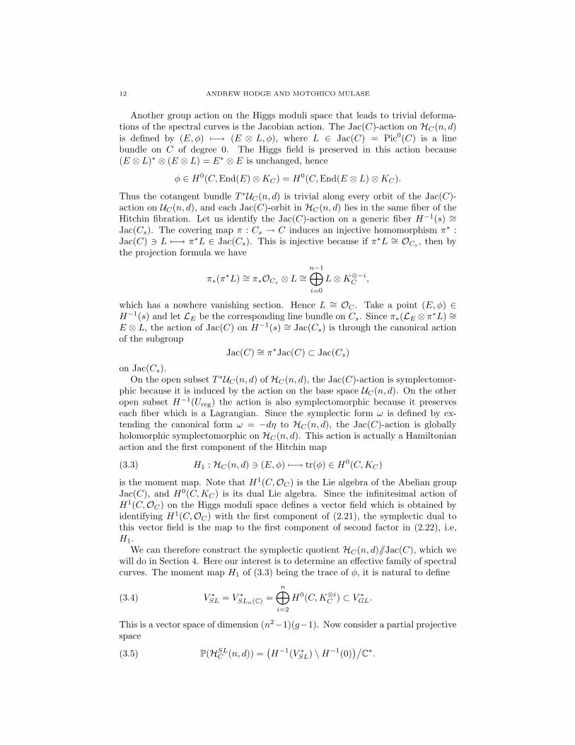
Another group action on the Higgs moduli space that leads to trivial deforma-tions of the spectral curves is the Jacobian action. The Jac(C)-action on HC(n, d)is defined by (E, φ) 7−→ (E ⊗ L, φ), where L ∈ Jac(C) = Pic0(C) is a linebundle on C of degree 0. The Higgs field is preserved in this action because(E ⊗ L)∗ ⊗ (E ⊗ L) = E∗ ⊗ E is unchanged, hence
φ ∈ H0(C,End(E)⊗KC) = H0(C,End(E ⊗ L)⊗KC).
Thus the cotangent bundle T ∗UC(n, d) is trivial along every orbit of the Jac(C)-action on UC(n, d), and each Jac(C)-orbit in HC(n, d) lies in the same fiber of theHitchin fibration. Let us identify the Jac(C)-action on a generic fiber H−1(s) ∼=Jac(Cs). The covering map π : Cs → C induces an injective homomorphism π∗ :Jac(C) 3 L 7−→ π∗L ∈ Jac(Cs). This is injective because if π∗L ∼= OCs , then bythe projection formula we have
π∗(π∗L) ∼= π∗OCs ⊗ L ∼=n−1⊕i=0
L⊗K⊗−iC ,
which has a nowhere vanishing section. Hence L ∼= OC . Take a point (E, φ) ∈H−1(s) and let LE be the corresponding line bundle on Cs. Since π∗(LE ⊗ π∗L) ∼=E ⊗ L, the action of Jac(C) on H−1(s) ∼= Jac(Cs) is through the canonical actionof the subgroup
Jac(C) ∼= π∗Jac(C) ⊂ Jac(Cs)
on Jac(Cs).On the open subset T ∗UC(n, d) of HC(n, d), the Jac(C)-action is symplectomor-
phic because it is induced by the action on the base space UC(n, d). On the otheropen subset H−1(Ureg) the action is also symplectomorphic because it preserveseach fiber which is a Lagrangian. Since the symplectic form ω is defined by ex-tending the canonical form ω = −dη to HC(n, d), the Jac(C)-action is globallyholomorphic symplectomorphic on HC(n, d). This action is actually a Hamiltonianaction and the first component of the Hitchin map
(3.3) H1 : HC(n, d) 3 (E, φ) 7−→ tr(φ) ∈ H0(C,KC)
is the moment map. Note that H1(C,OC) is the Lie algebra of the Abelian groupJac(C), and H0(C,KC) is its dual Lie algebra. Since the infinitesimal action ofH1(C,OC) on the Higgs moduli space defines a vector field which is obtained byidentifying H1(C,OC) with the first component of (2.21), the symplectic dual tothis vector field is the map to the first component of second factor in (2.22), i.e,H1.
We can therefore construct the symplectic quotient HC(n, d)//Jac(C), which wewill do in Section 4. Here our interest is to determine an effective family of spectralcurves. The moment map H1 of (3.3) being the trace of φ, it is natural to define
(3.4) V ∗SL = V ∗SLn(C) =n⊕i=2
H0(C,K⊗iC ) ⊂ V ∗GL.
This is a vector space of dimension (n2−1)(g−1). Now consider a partial projectivespace
(3.5) P(HSLC (n, d)) =(H−1(V ∗SL) \H−1(0)
)/C∗.

HITCHIN SYSTEMS, SPECTRAL CURVES, AND KP EQUATIONS 13
This is no longer a holomorphic symplectic manifold, yet the Hitchin fibrationnaturally descends to a generically Jacobian fibration
(3.6) PH : P(HSLC (n, d)) −→ Pw(V ∗SL)
over the weighted projective space of V ∗SL defined by the restriction of (3.1) on V ∗SL.We now claim
Theorem 3.1 (Effective Jacobian fibration). The Jacobian fibration
PH : P(HSLC (n, d)) −→ Pw(V ∗SL)
is generically effective.
The rest of this section is devoted to the proof of this theorem. The state-ment is equivalent to the claim that the family of deformations of spectral curvesparametrized by Pw(V ∗SL) is effective. Let s ∈ V ∗SL be a point for which the spectralcurve Cs is non-singular, and s the corresponding point of Pw(V ∗SL). We wish toshow that the Kodaira-Spencer map
Ts Pw(V ∗SL) −→ H1(Cs, T Cs)
is injective, where T X denotes the tangent sheaf of X.The spectral curve Cs of (2.11) is the divisor of T ∗C defined by the section
det(τ − φ) ∈ H0(T ∗C, π∗K⊗nC ),
where τ is the tautological section of π∗KC on T ∗C. Let Ns denote the normalsheaf of Cs in T ∗C. Since KT∗C = Λ2(T ∗C) ∼= OT∗C by the holomorphic symplecticform ωC = −dτ , we have
Ns ∼= KCs∼= π∗K⊗nC .
From0 −−−−→ T Cs −−−−→ T T ∗C|Cs −−−−→ Ns −−−−→ 0,
we obtain
(3.7)0 −−−−→ H0(Cs, T T ∗C) ι−−−−→ H0(Cs,Ns)
κ−−−−→ H1(Cs, T Cs)
−−−−→ H1(Cs, T T ∗C) −−−−→ H1(Cs,Ns).
Since
H0(Cs,Ns) ∼= H0(C, π∗KCs) ∼=n⊕i=1
H0(C,K⊗iC ) = V ∗GL,
the homomorphism κ is the Kodaira-Spencer map for the deformations of spectralcurves on V ∗GL. We thus need to identify the image of ι. We note that the tangentsheaf and the cotangent sheaf are isomorphic on the total space of the cotangentbundle T ∗C, i.e., T T ∗C ∼= Λ1(T ∗C).
Proposition 3.2. We have the following isomorphisms:
(3.8)
H0(T ∗C,Λ0(T ∗C)) ∼= CH0(T ∗C,Λ1(T ∗C)) ∼= H0(C,KC)⊕ C · τH0(T ∗C,Λ2(T ∗C)) ∼= C.
14 ANDREW HODGE AND MOTOHICO MULASE
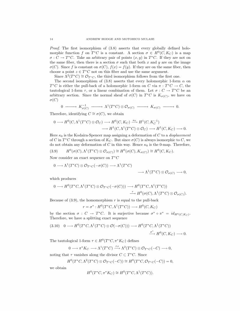
Proof. The first isomorphism of (3.8) asserts that every globally defined holo-morphic function f on T ∗C is a constant. A section σ ∈ H0(C,KC) is a mapσ : C → T ∗C. Take an arbitrary pair of points (x, y) in T ∗C. If they are not onthe same fiber, then there is a section σ such that both x and y are on the imageσ(C). Since f is constant on σ(C), f(x) = f(y). If they are on the same fiber, thenchoose a point z ∈ T ∗C not on this fiber and use the same argument.
Since Λ2(T ∗C) ∼= OT∗C , the third isomorphism follows from the first one.The second isomorphism of (3.8) asserts that every holomorphic 1-form α on
T ∗C is either the pull-back of a holomorphic 1-form on C via π : T ∗C → C, thetautological 1-form τ , or a linear combination of them. Let σ : C → T ∗C be anarbitrary section. Since the normal sheaf of σ(C) in T ∗C is Kσ(C), we have onσ(C)
0 −−−−→ K−1σ(C) −−−−→ Λ1(T ∗C)⊗Oσ(C) −−−−→ Kσ(C) −−−−→ 0.
Therefore, identifying C ∼= σ(C), we obtain
0 −→ H0(C,Λ1(T ∗C)⊗OC) −→ H0(C,KC) κ0−→ H1(C,K−1C )
−→ H1(C,Λ1(T ∗C)⊗OC) −→ H1(C,KC) −→ 0.
Here κ0 is the Kodaira-Spencer map assigning a deformation of C to a displacementof C in T ∗C through a section of KC . But since σ(C) is always isomorphic to C, wedo not obtain any deformation of C in this way. Hence κ0 is the 0-map. Therefore,
(3.9) H0(σ(C),Λ1(T ∗C)⊗Oσ(C)) ∼= H0(σ(C),Kσ(C)) ∼= H0(C,KC).
Now consider an exact sequence on T ∗C
0 −→ Λ1(T ∗C)⊗OT∗C(−σ(C)) −→ Λ1(T ∗C)
−→ Λ1(T ∗C)⊗Oσ(C) −→ 0,
which produces
0 −→ H0(T ∗C,Λ1(T ∗C)⊗OT∗C(−σ(C))) −→ H0(T ∗C,Λ1(T ∗C))r−→ H0(σ(C),Λ1(T ∗C)⊗Oσ(C)).
Because of (3.9), the homomorphism r is equal to the pull-back
r = σ∗ : H0(T ∗C,Λ1(T ∗C)) −→ H0(C,KC)
by the section σ : C → T ∗C. It is surjective because σ∗ ◦ π∗ = idH0(C,KC).Therefore, we have a splitting exact sequence
(3.10) 0 −→ H0(T ∗C,Λ1(T ∗C)⊗O(−σ(C))) −→ H0(T ∗C,Λ1(T ∗C))σ∗−→ H0(C,KC) −→ 0.
The tautological 1-form τ ∈ H0(T ∗C, π∗KC) defines
0 −→ π∗KC −→ Λ1(T ∗C) ∧τ−→ Λ2(T ∗C)⊗OT∗C(−C) −→ 0,
noting that τ vanishes along the divisor C ⊂ T ∗C. Since
H0(T ∗C,Λ2(T ∗C)⊗OT∗C(−C)) ∼= H0(T ∗C,OT∗C(−C)) = 0,
we obtainH0(T ∗C, π∗KC) ∼= H0(T ∗C,Λ1(T ∗C)).
HITCHIN SYSTEMS, SPECTRAL CURVES, AND KP EQUATIONS 15
Take α ∈ H0(T ∗C,Λ1(T ∗C)⊗OT∗C(−C)) ∼= H0(T ∗C, π∗KC(−C)). Then
α/τ ∈ H0(T ∗C, π∗KC(−C)⊗ π∗K−1C (C)) ∼= H0(T ∗C,OT∗C) ∼= C.
Therefore, α is a constant multiple of τ , and we have obtained
(3.11) H0(T ∗C,Λ1(T ∗C)⊗OT∗C(−C)) ∼= C.From (3.10) and (3.11), we conclude that
H0(T ∗C,Λ1(T ∗C)) ∼= H0(C,KC)⊕ C · τ.�
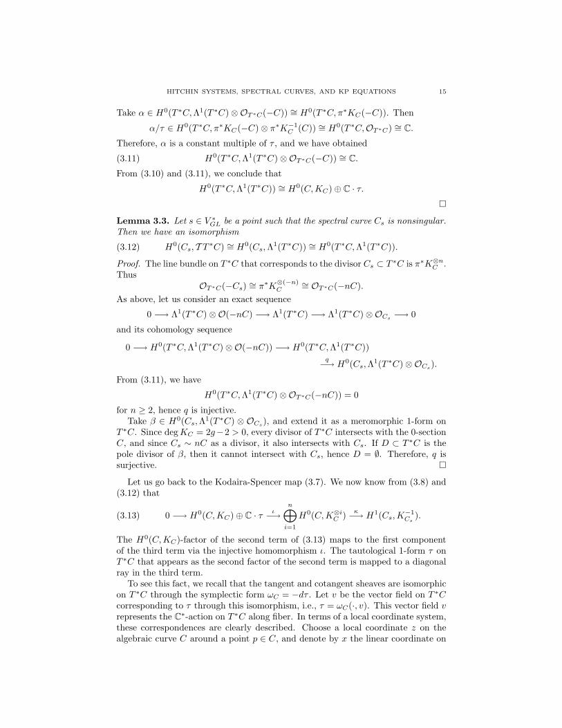
Lemma 3.3. Let s ∈ V ∗GL be a point such that the spectral curve Cs is nonsingular.Then we have an isomorphism
(3.12) H0(Cs, T T ∗C) ∼= H0(Cs,Λ1(T ∗C)) ∼= H0(T ∗C,Λ1(T ∗C)).
Proof. The line bundle on T ∗C that corresponds to the divisor Cs ⊂ T ∗C is π∗K⊗nC .Thus
OT∗C(−Cs) ∼= π∗K⊗(−n)C
∼= OT∗C(−nC).As above, let us consider an exact sequence
0 −→ Λ1(T ∗C)⊗O(−nC) −→ Λ1(T ∗C) −→ Λ1(T ∗C)⊗OCs −→ 0
and its cohomology sequence
0 −→ H0(T ∗C,Λ1(T ∗C)⊗O(−nC)) −→ H0(T ∗C,Λ1(T ∗C))q−→ H0(Cs,Λ1(T ∗C)⊗OCs).
From (3.11), we have
H0(T ∗C,Λ1(T ∗C)⊗OT∗C(−nC)) = 0
for n ≥ 2, hence q is injective.Take β ∈ H0(Cs,Λ1(T ∗C) ⊗ OCs), and extend it as a meromorphic 1-form on
T ∗C. Since degKC = 2g−2 > 0, every divisor of T ∗C intersects with the 0-sectionC, and since Cs ∼ nC as a divisor, it also intersects with Cs. If D ⊂ T ∗C is thepole divisor of β, then it cannot intersect with Cs, hence D = ∅. Therefore, q issurjective. �
Let us go back to the Kodaira-Spencer map (3.7). We now know from (3.8) and(3.12) that
(3.13) 0 −→ H0(C,KC)⊕ C · τ ι−→n⊕i=1
H0(C,K⊗iC ) κ−→ H1(Cs,K−1Cs
).
The H0(C,KC)-factor of the second term of (3.13) maps to the first componentof the third term via the injective homomorphism ι. The tautological 1-form τ onT ∗C that appears as the second factor of the second term is mapped to a diagonalray in the third term.
To see this fact, we recall that the tangent and cotangent sheaves are isomorphicon T ∗C through the symplectic form ωC = −dτ . Let v be the vector field on T ∗Ccorresponding to τ through this isomorphism, i.e., τ = ωC(·, v). This vector field vrepresents the C∗-action on T ∗C along fiber. In terms of a local coordinate system,these correspondences are clearly described. Choose a local coordinate z on thealgebraic curve C around a point p ∈ C, and denote by x the linear coordinate on
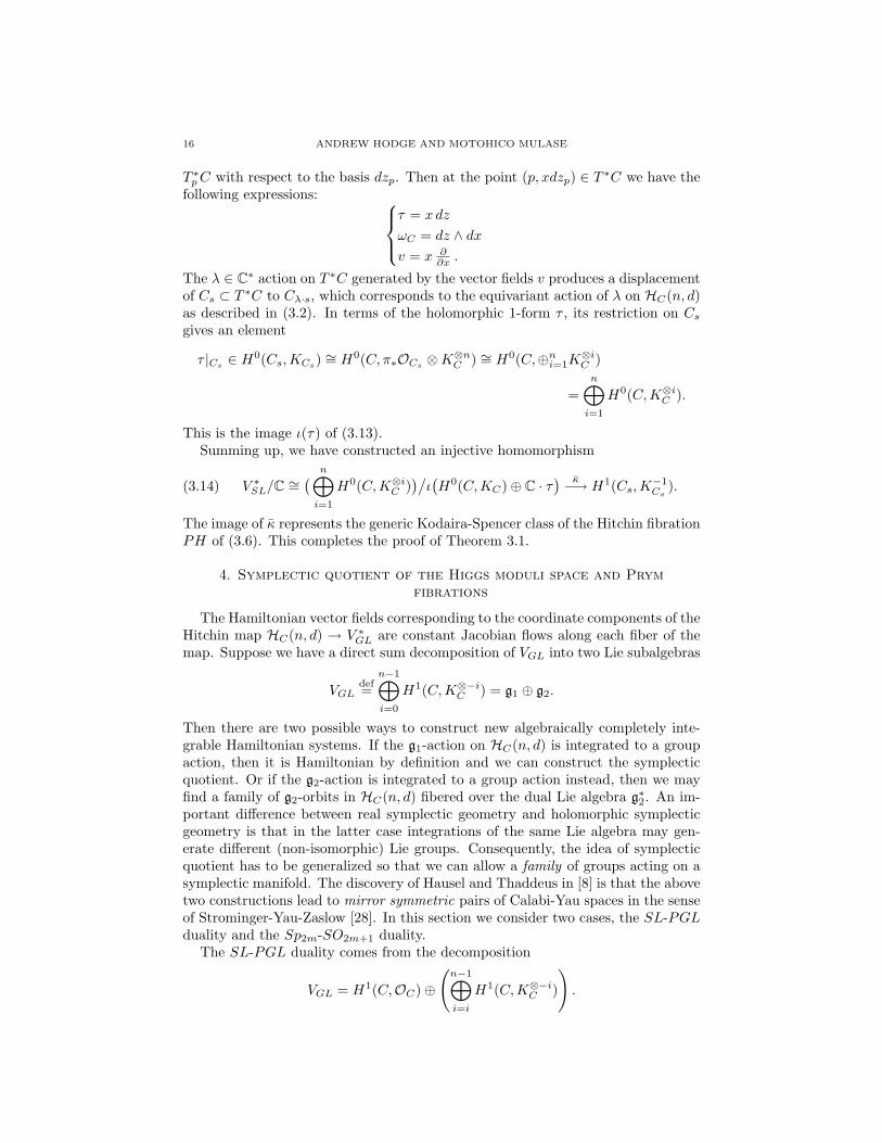
16 ANDREW HODGE AND MOTOHICO MULASE
T ∗pC with respect to the basis dzp. Then at the point (p, xdzp) ∈ T ∗C we have thefollowing expressions:
τ = x dz
ωC = dz ∧ dxv = x ∂
∂x .
The λ ∈ C∗ action on T ∗C generated by the vector fields v produces a displacementof Cs ⊂ T ∗C to Cλ·s, which corresponds to the equivariant action of λ on HC(n, d)as described in (3.2). In terms of the holomorphic 1-form τ , its restriction on Csgives an element
τ |Cs ∈ H0(Cs,KCs) ∼= H0(C, π∗OCs ⊗K⊗nC ) ∼= H0(C,⊕ni=1K⊗iC )
=n⊕i=1
H0(C,K⊗iC ).
This is the image ι(τ) of (3.13).Summing up, we have constructed an injective homomorphism
(3.14) V ∗SL/C ∼=( n⊕i=1
H0(C,K⊗iC ))/ι(H0(C,KC)⊕ C · τ
) κ−→ H1(Cs,K−1Cs
).
The image of κ represents the generic Kodaira-Spencer class of the Hitchin fibrationPH of (3.6). This completes the proof of Theorem 3.1.
4. Symplectic quotient of the Higgs moduli space and Prymfibrations
The Hamiltonian vector fields corresponding to the coordinate components of theHitchin map HC(n, d) → V ∗GL are constant Jacobian flows along each fiber of themap. Suppose we have a direct sum decomposition of VGL into two Lie subalgebras
VGLdef=
n−1⊕i=0
H1(C,K⊗−iC ) = g1 ⊕ g2.
Then there are two possible ways to construct new algebraically completely inte-grable Hamiltonian systems. If the g1-action on HC(n, d) is integrated to a groupaction, then it is Hamiltonian by definition and we can construct the symplecticquotient. Or if the g2-action is integrated to a group action instead, then we mayfind a family of g2-orbits in HC(n, d) fibered over the dual Lie algebra g∗2. An im-portant difference between real symplectic geometry and holomorphic symplecticgeometry is that in the latter case integrations of the same Lie algebra may gen-erate different (non-isomorphic) Lie groups. Consequently, the idea of symplecticquotient has to be generalized so that we can allow a family of groups acting on asymplectic manifold. The discovery of Hausel and Thaddeus in [8] is that the abovetwo constructions lead to mirror symmetric pairs of Calabi-Yau spaces in the senseof Strominger-Yau-Zaslow [28]. In this section we consider two cases, the SL-PGLduality and the Sp2m-SO2m+1 duality.
The SL-PGL duality comes from the decomposition
VGL = H1(C,OC)⊕
(n−1⊕i=i
H1(C,K⊗−iC )
).

HITCHIN SYSTEMS, SPECTRAL CURVES, AND KP EQUATIONS 17
Obviously, the vector fields generated by the H1(C,OC)-action are integrable to theJac(C)-action everywhere on HC(n, d). Therefore, we do have the usual symplecticquotient mod Jac(C). On the other hand, the integration of the other Lie algebra
VSLdef=
n−1⊕i=i
H1(C,K⊗−iC )
produces different Lie groups, called Prym varieties, along each fiber of the Hitchinfibration.
The spectral covering π : Cs → C induces two group homomorphisms dual toone another, the pull-back π∗ and the norm map Nmπ defined by
(4.1)π∗ : Jac(C) 3 L 7−→ π∗L ∈ Jac(Cs)
Nmπ : Jac(Cs) 3 L 7−→ det(π∗L)⊗ det(π∗OCs)−1 ∈ Jac(C).
In terms of divisors the norm map can be defined alternatively by
Pic(Cs) 3∑p∈Cs
m(p) · p 7−→∑p∈Cs
m(p) · π(p) ∈ Jac(C).
The Prym variety and the dual Prym variety
(4.2)Prym(Cs/C) def= Ker(Nmπ)
Prym∗(Cs/C) def= Jac(Cs)/π∗Jac(C)
constructed by using these homomorphisms are Abelian varieties of dimensiong(Cs)− g(C) and are dual to one another. The algebraically completely integrableHamiltonian systems with these Abelian fibrations, that are naturally constructedfrom HC(n, d), then become SYZ-mirror symmetric.
We have shown in Section 3 that the Jac(C)-action on HC(n, d) is Hamiltonian.So we can define the symplectic quotient
(4.3) PHC(n, d) def= HC(n, d)//Jac(C) = H−11 (0)/Jac(C).
This is a symplectic space of dimension 2(n2−1)(g−1) modeled by the moduli spaceof stable principal PGLn(C)-bundles on C [10, 11]. Since the Jac(C)-action onHC(n, d) preserves the Hitchin fibration, we have an induced Lagrangian fibration
(4.4) HPGL : PHC(n, d) −→ V ∗SL =n⊕i=2
H0(C,K⊗iC ).
It’s 0-fiber is H−1PGL(0) = UC(n, d)/Jac(C). Following [21] we denote by SUC(n, d)
the moduli space of stable vector bundles with a fixed determinant line bundle.This is a fiber of the determinant map
(4.5) UC(n, d) 3 E 7−→ detE ∈ Picd(C),
and is independent of the choice of the value of the determinant. Note that (4.5)is a non-trivial fiber bundle. The equivariant Jac(C)-action on (4.5) is given by
(4.6)
UC(n, d) ⊗L−−−−→ UC(n, d)
det
y ydet
Picd(C) −−−−→⊗L⊗n
Picd(C)
L ∈ Jac(C).

18 ANDREW HODGE AND MOTOHICO MULASE
The isotropy subgroup of the Jac(C)-action on UC(n, d) is the group of n-torsionpoints
(4.7) Jn(C) def= {L ∈ Jac(C) |L⊗n = OC} ∼= H1(C,Z/nZ),
since E ⊗ L ∼= E implies det(E) ⊗ L⊗n ∼= det(E). Choose a reference line bundleL0 ∈ Picd(C) and consider a degree n covering
ν : Picd(C) 3 L⊗ L0 7−→ L⊗n ⊗ L0 ∈ Picd(C), L ∈ Jac(C).
Then the pull-back bundle ν∗UC(n, d) on Picd(C) becomes trivial:
ν∗UC(n, d) = Picd(C)× SUC(n, d).
The quotient of this product by the diagonal action of Jn(C) is the original modulispace:
(4.8)(Picd(C)× SUC(n, d)
)/Jn(C) ∼= UC(n, d).
It is now clear that
UC(n, d)/Jac(C) ∼= SUC(n, d)/Jn(C).
What are the other fibers of (4.4)? Let s ∈ V ∗SL ∩Ureg be a point such that Cs isnon-singular. We have already noted that the covering map π : Cs → C induces aninjective homomorphism π∗ : Jac(C) 3 L 7−→ π∗L ∈ Jac(Cs). Therefore, the fiberH−1PGL(s) is isomorphic to the dual Prym variety Prym∗(Cs/C). Similarly to the
equivariant action (4.6), we have
(4.9)
Jac(Cs)⊗L−−−−→ Jac(Cs)
Nm
y yNm
Jac(C) −−−−→⊗L⊗n
Jac(C)
L ∈ Jac(C).
By the same argument of (4.8), we obtain
(4.10)(Prym(Cs/C)× Jac(C)
)/Jn(C) ∼= Jac(Cs).
From (4.2) and (4.10), it follows that
Prym∗(Cs/C) = Prym(Cs/C)/Jn(C).
We have thus established
Theorem 4.1 ([11, 12]). The natural fibration
HPGL : PHC(n, d) −→ V ∗SL =n⊕i=2
H0(C,K⊗iC )
of (4.4) is a Lagrangian dual Prym fibration with respect to the canonical holomor-phic symplectic form ω on PHC(n, d).
We recall that the Higgs moduli space HC(n, d) contains the cotangent bundleT ∗UC(n, d) as an open dense subspace, and that the holomorphic symplectic formω is the canonical symplectic form on this cotangent bundle. Similarly, we can showthe following
HITCHIN SYSTEMS, SPECTRAL CURVES, AND KP EQUATIONS 19
Proposition 4.2. The symplectic form ω on PHC(n, d) given by the symplecticquotient is the canonical cotangent symplectic form on the cotangent bundle
T ∗(SUC(n, d)/Jn(C)
)⊂ PHC(n, d).
Proof. Let E be a stable vector bundle on C. The exact sequence
0 −−−−→ OC −−−−→ End(E) −−−−→ Q = End(E)/OC −−−−→ 0
induces a cohomology sequence
0 −−−−→ H1(C,OC) −−−−→ H1(C,End(E)).
Therefore,
TE(SUC(n, d)/Jn(C)
) ∼= H1(C,End(E))/H1(C,OC).
Dualizing the situation, we have
0 −→ End0(E)⊗KC −→ End(E)⊗KCtr−→ KC −→ 0,
where End0(E) is the sheaf of traceless endomorphisms of E. We then have
0 −→ H0(C,End0(E)⊗KC) −→ H0(C,End(E)⊗KC)tr−→ H0(C,KC) −→ 0.
The trace homomorphism is globally surjective because OC is contained in End(E).Hence
T ∗E(SUC(n, d)/Jn(C)
) ∼= H0(C,End0(E)⊗KC).
Since the moment map H1 of (3.3) is the trace map, we conclude that the symplecticform ω on the symplectic quotient PHC(n, d) is the canonical cotangent symplecticform on the cotangent bundle
T ∗(SUC(n, d)/Jn(C)
).
�
The other reduction of HC(n, d) consisting of the VSL-orbits is the moduli spaceSHC(n, d) of stable Higgs bundles (E, φ) with a fixed determinant det(E) ∼= L andtraceless Higgs fields
φ ∈ H0(C,End0(E)⊗KC).
This moduli space is modeled by the moduli space of stable principal SLn(C)-bundles on C and has dimension 2(n2−1)(g−1). The cotangent bundle T ∗SUC(n, d)is an open dense subspace of SHC(n, d). Since tr(φ) = 0, the Hitchin fibration Hof (2.9) naturally restricts to
(4.11) HSL : SHC(n, d) −→ V ∗SL =n⊕i=2
H0(C,K⊗iC ).
The 0-fiber is H−1SL(0) = SHC(n, d). For a generic s ∈ V ∗SL such that Cs is non-
singular, the fiber H−1SL(s) is the subset of H−1(s) ∼= Jac(Cs) consisting of Higgs
bundles (E, φ) such that det(E) = L is fixed and det(x − φ) = s. Therefore,H−1SL(s) ∼= Prym(Cs/C).By comparing PHC(n, d) and SHC(n, d), we find that
(4.12) SHC(n, d)/Jn(C) ∼= PHC(n, d),
20 ANDREW HODGE AND MOTOHICO MULASE
where the Jn(C)-action on SHC(n, d) is defined by E 7→ E ⊗ L for L ∈ Jn(C).Since Jn(C) is a finite group and PHC(n, d) is a holomorphic symplectic variety,we can define a holomorphic symplectic form ω on SHC(n, d) via the pull-back ofthe projection
SHC(n, d) −→ SHC(n, d)/Jn(C).
Obviously ω agrees with the canonical cotangent symplectic form on T ∗SUC(n, d).Therefore,
Theorem 4.3 ([11, 12]). The fibration
HSL : SHC(n, d) −→ V ∗SL =n⊕i=2
H0(C,K⊗iC )
is a Lagrangian Prym fibration with respect to the canonical holomorphic symplecticform ω on SHC(n, d).
Hausel and Thaddeus [8] shows that
Theorem 4.4 (Theorem (3.7) in [8]). The two fibrations
SHC(n, d)HSL
%%JJJJJJJJJPHC(n, d)
HPGL
yytttttt
tttt
V ∗SL
are mirror symmetric in the sense of Strominger-Yau-Zaslow [28].
The effectiveness of the family of Prym and dual Prym varieties can be estab-lished by the same method of Section 3. Let us define partial projective modulispaces
P(PHC(n, d)) def=(PHC(n, d) \H−1
PGL(0))/
C∗
andP(SHC(n, d)) def=
(SHC(n, d) \H−1
SL(0))/
C∗.The induced Hitchin maps are denoted by
(4.13)PHPGL : P(PHC(n, d)) −→ Pw(V ∗SL)
PHSL : P(SHC(n, d)) −→ Pw(V ∗SL).
We have the following
Theorem 4.5. The Prym and dual Prym fibrations
PHSL : P(SHC(n, d)) −→ Pw(V ∗SL)
PHPGL : P(PHC(n, d)) −→ Pw(V ∗SL)
are generically effective.
For the case of Sp2m(C)-Hitchin systems, we consider Lie subalgebras
(4.14)
g =m−1⊕i=0
H1(C,K⊗−2i
C
)VSp =
m−1⊕i=0
H1(C,K⊗−2i−1
C
),

HITCHIN SYSTEMS, SPECTRAL CURVES, AND KP EQUATIONS 21
and a direct sum decomposition
(4.15) VGL2m = g⊕ VSp.
This time the Hamiltonian flows on HC(n, d) generated by elements of g do notform a group action. However, if we restrict our attention to points of Ureg∩V ∗Sp asin (2.27), then the integral of the Lie algebra action becomes a group action. Recallthat the spectral curve Cs has an involution induced by ε of (2.26). We denote by
(4.16) r : Cs → C ′s = Cs/〈ε〉
the natural projection. It is ramified at the intersection of Cs with the 0-section ofT ∗C, which is the divisor of π∗KC on Cs of degree 4m(g − 1). Therefore, we findthe genus of C ′s by the Riemann-Hurwitz formula:
(4.17) g(C ′s) = m(2m− 1)(g − 1) + 1 = dim g.
Since H0(C ′s, r∗OCs) has a nowhere vanishing section, we have
(4.18) 0 −−−−→ OC′s −−−−→ r∗OCs −−−−→ N−1 −−−−→ 0
with a line bundle N on C ′s of degree 2m(g − 1). Note that
N⊗2 = det(r∗OCs)⊗−2 ∼= Nmr(π∗KC),
hence N is a square root of the branch divisor Nmr(π∗KC) of the covering r. Theexact sequence (4.18) gives
(4.19) H1(Cs,OCs) ∼= H1(C ′s,OC′s)⊕H1(C ′s, N
−1),
and the projection to the first factor is the differential of the norm map
Nmr : Jac(Cs) 3 L 7−→ det(r∗L)⊗ det(r∗OCs)−1 ∈ Jac(C ′s).
The construction of the Sp-Hitchin system of Proposition 2.4 is to reduce the GL-Hitchin system HC(2m, 2m(g − 1)) by finding the right fibration of groups. Alongthe fixed-point-set of the Serre duality on this Higgs moduli space, the action of VSpgenerates the Prym fibration {Prym(Cs/C ′s)}s∈V ∗Sp since the condition L∗0 ∼= ε∗L0
on Cs is the same as L0 ∈ Prym(Cs/C ′s). Comparing (4.15) and (4.19), we have
H1(C ′s,OC′s) ∼= g and H1(C ′s, N−1) ∼= VSp.
The dual fibration is the result of a kind of symplectic quotient ofHC(2m, 2m(g−1)) by g. In this quotient we restrict the Hitchin fibration to the 0-fiber of
g∗ =m⊕i=1
H0(C,K⊗2i−1
C
),
and then take the quotient of each fiber by the Lie group Jac(C ′s) of g. The resultis the dual Prym fibration with a fiber
Prym∗(Cs/C ′s) = Jac(Cs)/Jac(C ′s) = Prym(Cs/C ′s)/J2(C ′s)
over each s ∈ V ∗Sp, where J2(C ′s) denotes the group of 2-torsion points of Jac(C ′s).

22 ANDREW HODGE AND MOTOHICO MULASE
5. Hitchin’s integrable systems and the KP equations
The partial projective Hitchin fibration
PH : P(HSLC (n, d))→ Pw(V ∗SL)
is a generically effective Jacobian fibration. In this section we embed P(HSLC (n, d))into a quotient of the Sato Grassmannian. There is also a natural embedding ofHC(n, n(g − 1)) into a relative Grassmannian of [2, 4, 22, 23]. We show that thelinear Jacobian flows on the Hitchin integrable system (HC(n, n(g − 1)), ω,H) areexactly the KP equations on the Grassmannian via this second embedding.
Following Quandt [23], we define
Definition 5.1 (Sato Grassmannian). Let n be a positive integer. The Sato Grass-mannian Grn is a functor from the category of schemes to the small category ofsets. It assigns to every scheme S a set Grn(S) consisting of quasi-coherent OS-submodules W of OS((z))⊕n such that both the kernel and the cokernel of the naturalhomomorphism
(5.1) 0 −→ Ker(γW ) −→WγW−→ OS((z))⊕n
/OS [[z]]⊕n −→ Coker(γW ) −→ 0
are coherent OS modules. We refer to this condition simply the Fredholm condition.Here we denote by OS [[z]] the ring of formal power series in z with coefficients inOS, and OS((z)) = OS [[z]] +OS [z−1].
Remark 5.1. A more general and powerful theory of relative Sato Grassmanni-ans has been recently established by Plaza Martın [22]. It would be an interestingproject to study possible relations between [22] and the geometric Langlands cor-respondence.
Remark 5.2. The Grassmannian Grn(C) defined over the point scheme Spec(C)has the structure of an infinite-dimensional pro-ind scheme over C. If S is ir-reducible, then Grn(S) is a disjoint union of an infinite number of componentsindexed by the Grothendieck group K(S):
(5.2) index : Grn(S) 3W 7−→ index(γW ) def= Ker(γW )− Coker(γW ) ∈ K(S).
Remark 5.3. The big cell is the open subscheme of the index 0 piece of theGrassmannian Gr0
n(S) consisting of W ’s such that γW is an isomorphism. This isthe stage where the Lax and Zakharov-Shabat formalisms of integrable nonlinearpartial differential equations, such as KP, KdV, and many other equations, areinterpreted as infinite-dimensional dynamical systems [24, 25]. The fundamentalresult is the identification (6.17) of the big cell with the group of 0-th order monicpseudo-differential operators [16, 23, 24, 25].
Remark 5.4. The above W is a closed subset of OS((z))⊕n with respect to thetopology defined by the filtration
· · · ⊃ zν−1 · OS [[z]]⊕n ⊃ zν · OS [[z]]⊕n ⊃ zν+1 · OS [[z]]⊕n ⊃ · · · .
One of the consequences of the Fredholm condition is that
(5.3) W ∩ zν · OS [[z]]⊕n = 0 for ν >> 0.

HITCHIN SYSTEMS, SPECTRAL CURVES, AND KP EQUATIONS 23
Consider the group
(5.4) Γn(S) = O×S ·
1
1. . .
1
+ z ·
OS [[z]]
OS [[z]]. . .
OS [[z]]
consisting of n × n invertible diagonal matrices with entries in the ring of formalpower series whose constant term is scalar diagonal. It acts on Grn(S) by left-multiplication without fixed points. Indeed, let W ∈ Grn(S) and c+ γ ∈ O×S · In +z · OS [[z]]⊕n satisfy that W = (c + γ) ·W . This means that γ · w ∈ W for everyw ∈ W since W is an OS-module. Since γ ∈ z · OS [[z]]⊕n, it then contradicts to(5.3) unless γ = 0. The quotient Grassmannian
(5.5) Zndef= Grn/Γn
is a smooth infinite-dimensional scheme. We denote by W the point of Zn corre-sponding to W ∈ Grn.
The tangent space TWGrn of the Sato Grassmannian at W is given by the spaceof continuous OS-homomorphisms
TWGrn = HomOS(W,OS((z))⊕n/W
).
The tangent space to Zn is then given by
(5.6) TWZn∼= HomOS
(W,OS((z))⊕n
/(Γn ·W )
).
This expression does not depend on the choice of the lift W ∈ Grn of W ∈ Zn.Every element a ∈ OS((z))⊕n defines a homomorphism
KP (a)W : W 3 w 7−→ a · w ∈ OS((z))⊕n/
(Γn ·W )
through the left multiplication as a diagonal matrix, which in turn determines aglobal vector field
OS((z))⊕n 3 a 7−→ KP (a) ∈ H0(Zn, TZn).
We call KP (a) the n-component KP flow associated with a. As explained in [16,17, 19, 23], the quotient of the index zero Grassmannian Z0
n is naturally identifiedwith the set of Lax operators (6.18), and the action of OS((z))⊕n on a Lax operatoris written as an infinite system of nonlinear partial differential equations called Laxequations. This system for the case of S = Spec(C) is the n-component Kadomtsev-Petviashvili hierarchy [16].
Associated to the Hitchin fibration H : HC(n, d) → V ∗GL we have a family ofspectral curves:
(5.7) CV ∗GL(n, d)
F %%LLLLLLLLLLinclusion // T ∗C × V ∗GL
p2xxqqqqqqqqqqq
V ∗GL
Here the fiber F−1(s) of s ∈ V ∗GL is the spectral curve Cs ⊂ T ∗C × {s}, and p2
is the projection to the second factor. We note that the ramification points of thecovering π : Cs → C are determined by the resultant of the defining equation
(5.8) xn + s1xn−1 + · · ·+ sn = 0

24 ANDREW HODGE AND MOTOHICO MULASE
of Cs and its derivative
(5.9) nxn−1 + (n− 1)s1xn−1 + · · ·+ sn−1 = 0.
For every s ∈ V ∗GL, we denote by Res(s) this resultant. The Sylvester matrix ofthese polynomials (5.8) and (5.9) show that
Res(s) ∈ H0(C,K⊗n(n−1)C ).
Since the linear system |KC | is base-point-free, for every choice of p ∈ C, the subset
(5.10) Up = {s ∈ V ∗GL | Cs is non-singular and π : Cs → C is unramified at p}is Zariski open in V ∗GL.
Theorem 5.5. There is a rational map
µ : P(HSLC (n, d)) −→ Zd−n(g−1)n (C)
of the partial projective moduli space of Higgs bundles into the quotient Grassman-nian of index d− n(g− 1). This map is generically injective. At a general point ofthe image of the embedding the n-component KP flows defined on Zn(C) are tangentto the Hitchin fibration PH : P(HSLC (n, d)) −→ Pw(V ∗SL).
Proof. A point of the partial projective Higgs moduli space represents an isomor-phism class of spectral data (π : Cs → C,L), where L is a line bundle on Cs ofdegree d + (n2 − n)(g − 1). Choose a point p ∈ C, a coordinate z of the formalcompletion Cp of C at p, and s ∈ Up ∩ V ∗SL so that Cs is non-singular and π isunramified over p. The formal coordinate z defines an identification OCp = C[[z]].We also choose a local trivialization of L around π−1(p), i.e., an isomorphism
(5.11) β : L|Cs,π−1(p)
∼−→ OCs,π−1(p)= C[[z]]⊕n.
Since the formal completion Cs,π−1(p) is the disjoint union of n copies of Cp, theformal coordinate z also defines an identification OCs,π−1(p)
= C[[z]]⊕n.Now define
W = β(H0(Cs \ π−1(p),L)) ⊂ C((z))⊕n,which is the set of meromorphic sections of L that are holomorphic on Cs \ π−1(p)and have finite poles at π−1(p). Since we have{
Ker(γW ) ∼= H0(Cs,L)Coker(γW ) ∼= H1(Cs,L),
W is a point of the Grassmannian Grd−n(g−1)n of index d− n(g − 1). The different
choice of the local trivialization β′ in (5.11) leads to an element β′ ◦ β−1 ∈ Γn.Therefore, the point W ∈ Z
d−n(g−1)n (C) is uniquely determined by (π : Cs →
C, p, z,L). Conversely this set of geometric data is uniquely determined by W (seeSection 5 of [16]). Thus the rational map µ is generically one-to-one. Notice thatthe Γn action on the Grassmannian is inessential from the geometric point of viewbecause it simply changes the local trivialization of (5.11).
The tangent space at a general point of P(HSLC (n, d)) is
H1(Cs,OCs)⊕ V ∗SL/C.Since the Kodaira-Spencer map (3.14) is injective, it suffices to show injectivity ofthe natural map

HITCHIN SYSTEMS, SPECTRAL CURVES, AND KP EQUATIONS 25
dµ : H1(Cs,OCs)⊕H1(Cs,K−1Cs
) −→ Hom(W,C((z))⊕n/W )
= TWGrn(C),
which is induced by the local trivialization of OCs and KC coming from the choiceof the local coordinate z. Using z, we define
AW = H0(Cs \ π−1(p),OCs) ⊂ C((z))⊕n,
which is a point of the Grassmannian satisfying{Ker(γAW ) ∼= H0(Cs,OCs)Coker(γAW ) ∼= H1(Cs,OCs).
We note that AW is a ring and W is an AW -module. Since
Coker(γAW ) =C((z))⊕n
AW + C[[z]]⊕n,
H1(Cs,OCs) is injectively mapped to Hom(W,C((z))⊕n/W ).The local coordinate z determines a local trivialization of KC
KC |Cp∼−→ OCp · dz
∼= OCp ,
and hence that of K−1Cs
K−1Cs
∣∣Cs,π−1(p)
∼−→(OCp
)⊕n· ∂∂z∼= C[[z]]⊕n · ∂
∂z.
This trivialization gives
H1(Cs,K−1Cs
) ∼=C((z))⊕n · ∂/∂z
DW + C[[z]]⊕n · ∂/∂z,
whereDW = H0(Cs \ π−1(p),K−1
Cs) ⊂ C((z))⊕n · ∂/∂z.
Note that s ∈ V ∗GL determines an element of H0(Cs,KCs) because
s ∈ V ∗GL =n⊕i=1
H0(C,K⊗iC ) ∼= H0(C, π∗π∗K⊗nC ) ∼= H0(Cs,KCs).
This holomorphic 1-form on Cs induces a homomorphism
L → L⊗KCs ,
or equivalently,K−1Cs⊗ L −→ L.
In terms of the local coordinate z, this homomorphism gives an action of DW onW . Since DW ·W ⊂ W , we conclude that H1(Cs,K−1
Cs) is injectively mapped to
TWGrn(C). In this construction H1(Cs,OCs) and H1(Cs,K−1Cs
) have no commonelement in TWGrn(C) except for 0. This establishes the injectivity of dµ.
In [16], it is proved that the orbit of the n-component KP flows starting from W
is isomorphic to Picd+(n2−n)(g−1)(Cs) (Theorem 5.8, [16]), which is the fiber of theHitchin map PH. This completes the proof of the theorem. �

26 ANDREW HODGE AND MOTOHICO MULASE
The above theorem does not say anything about the Hitchin integrable system,because the partial projective moduli space is not a symplectic manifold and we donot have any integrable systems on it. To directly compare the Jacobian flows of theHitchin systems and the KP flows, we use the relative Grassmannian of [23] definedon the scheme Up of (5.10). So let π−1(p) = {p1, . . . , pn}, and denote by zi = π∗(z)the formal coordinate of Cs,pi . Choose a linear coordinate system (h1, . . . , hN ) forV ∗GL as in (2.24). Recall that π∗OCs ∼= ⊕n−1
i=0 K⊗−iC , and from (2.21) we have
H1(Cs,OCs) ∼=n−1⊕i=0
H1(C,K⊗−iC ) = VGL.
Using the Cech cohomology computation based on the covering C = (C \{p})∪ Cp,we expand each hk ∈ VGL as
(5.12) hk =n∑i=1
∑j≥1
tijkz−ji , tijk ∈ C.
The n-component KP flows on the Grassmannian Grn(Up) is defined by a formalaction of
(5.13) exp
n∑i=1
∑j≥1
N∑k=1
tijkz−ji
.
For degree d = n(g − 1), we have the following:
Theorem 5.6. Let us choose a point p ∈ C, a formal coordinate z of Cp, and asquare root of the canonical sheaf K1/2
C . Then the fibration
CV ∗GL(n, n(g − 1))
F''OOOOOOOOOOOOπ // C × V ∗GL
p2zzttttttttt
V ∗GL
determines a point W ∈ Gr0n(Up). There is a birational map from HC(n, n(g−1)) to
the orbit of the n-component KP flows on the quotient Grassmannian Z0n(Up) start-
ing from W . The Hitchin integrable system on the Higgs moduli space HC(n, n(g−1)) is the pull-back of the n-component KP equations via this birational map.
Proof. We regard C, p, z, and K1/2C being defined over the trivial family C × V ∗GL.
There is a natural choice of a local trivialization of K1/2C on Cp determined by the
coordinate z. Note that
(5.14) K1/2 def= π∗(Kn/2C )
is a square root of the relative dualizing sheaf K = π∗(KnC) on
CV ∗GL(n, n(g − 1)).
Take an arbitrary point s ∈ Up. Since p ∈ C is a point of C at which π isunramified, the formal coordinate z determines a local trivialization of K1/2 alongπ−1(p) ⊂ CV ∗GL(n, n(g − 1)). Define
(5.15) W = H0(CV ∗GL(n, n(g − 1)) \ π−1(p),K1/2) ⊂ OUp((z))⊕n,
HITCHIN SYSTEMS, SPECTRAL CURVES, AND KP EQUATIONS 27
using this local trivialization. Since{Ker(γWs) ∼= H0(Cs,K
1/2Cs
)Coker(γWs
) ∼= H1(Cs,K1/2Cs
)
for each s ∈ Up, we have W ∈ Gr0n(Up). Let us analyze the action of (5.13) at W .
On each Cs, hk =∑tijkz
−ji defines an element of H1(Cs,OCs). The exponential
of (5.13) is the Lie integration map
(5.16) VGL ∼= H1(Cs,OCs)exp−→ H1(Cs,OCs)
/H1(Cs,Z) = Jac(Cs).
Therefore, the action of (5.13) at the point W produces simultaneous deformationsof the line bundle
(5.17) K1/2 7−→ K1/2 ⊗ exp
n∑i=1
∑j≥1
N∑k=1
tijkz−ji
on CV ∗GL(n, n(g − 1)). Consequently, the orbit of the n-component KP flows on
Z0n(Up) starting at W is naturally identified with the family of Picn
2(g−1)(Cs) onUp. Since the Hitchin fibration H : HC(n, n(g − 1)) → V ∗GL is also a family ofPicn
2(g−1)(Cs) on V ∗GL, we have a rational map from H : HC(n, n(g − 1)) to then-component KP orbit of W in Z0
n(Up).Recall that the Hitchin integrable system on H : HC(n, n(g − 1)) is the linear
Jacobian flows defined by the coordinate functions (h1, . . . , hN ). We note that thisis exactly what (5.17) gives. �
Remark 5.7. So far we have assumed that Cs is non-singular. Although it willnot be an Abelian variety, we can still define the Jacobian Jac(Cs) using (5.16)when the spectral curve Cs is singular. As long as we choose p ∈ C so thatπ−1(p) avoids the singular locus of Cs, the KP flows are well defined. Moreover,the theory of Heisenberg KP flows introduced in [1, 16] allows us to consider thecovering π : Cs → C right at a ramification point. It is more desirable to define theGrassmmanian over the whole V ∗GL and to deal with the entire family F : CV ∗GL →V ∗GL together with the moduli stack of Higgs bundles instead of the stable moduliwe have considered here, since the framework of the Sato Grassmannian allows usto consider all vector bundles on C and degenerated spectral curves. We refer to[4] for a study in this direction.
6. Serre duality and formal adjoint of pseudo-differentialoperators
In this section we analyze the Serre duality of Higgs bundles in terms of the lan-guage of the Sato Grassmannian, and identify the involution on the correspondingpseudo-differential operators.
The Krichever construction ([17, 19, 25]) assigns a point W of the Sato Grass-mannian,
(6.1) Grn(C) 3W = β(H0(C \ {p}, F )) ⊂ C((z))⊕n,
to a set of geometric data (C, p, z, F, β), where C is an irreducible algebraic curve,p ∈ C is a non-singular point, z is a formal parameter of the completion Cp, F is a

28 ANDREW HODGE AND MOTOHICO MULASE
torsion-free sheaf of rank n on C, and
β : F |Cp∼−→ O⊕n
Cp= C[[z]]⊕n
is a local trivialization of F around p. We continue to assume that C is non-singular,hence F is locally-free on C. As noted in Section 5, the choice of a local coordinatez automatically determines a local trivialization of KC :
(6.2) α : KC |Cp∼−→ OCp · dz
∼= OCp .
For every homomorphism ξ : F → KC , we have an element
β∗(ξ) def= α ◦ ξ ◦ β−1 ∈(O⊕nCp
)∗= O⊕n
Cp
that is determined by the commutative diagram
(6.3)
F |Cpξ−−−−→ KC |Cp
β
yo oyα
O⊕nCp
β∗(ξ)−−−−→ OCp .
Thus we have the canonical choice of the local trivialization
β∗ : F ∗ ⊗KC |Cp∼−→ O⊕n
Cp.
Definition 6.1 (Serre Dual). The Serre dual of the geometric date (C, p, z, F, β)is the set of data (C, p, z, F ∗ ⊗KC , β
∗).
To identify the counterpart of the Serre duality on the Sato Grassmannian, weintroduce a non-degenerate symmetric paring in C((z)) by
(6.4) 〈a(z), b(z)〉 =1
2πi
∮a(z)b(z)dz = the coefficient of z−1 in a(z)b(z),
and define
(6.5) 〈f(z), g(z)〉n =n∑i=1
〈fi(z), gi(z)〉, f(z), g(z) ∈ C((z))⊕n.
Lemma 6.1. Let W ∈ Grn(C) be a point of the Sato Grassmannian of index d.Then
W⊥ = {f ∈ C((z))⊕n | 〈f, w〉n = 0 for all w ∈W}is a point of Grn(C) of index −d. Moreover, we have
(6.6)
{Ker(γW )∗ ∼= Coker(γW⊥)Coker(γW )∗ ∼= Ker(γW⊥),
where γW is defined by the exact sequence
0 −→ Ker(γW ) −→WγW−→ C((z))⊕n/C[[z]]⊕n −→ Coker(γW ) −→ 0.
Proof. Take an element f ∈W⊥ ∩ C[[z]]⊕n. Then
〈f,W + C[[z]]⊕n〉n = 0.
Thus it induces a linear map
f : C((z))/
(W + C[[z]]⊕n) 3 g 7−→ 〈f, g〉n ∈ C,

HITCHIN SYSTEMS, SPECTRAL CURVES, AND KP EQUATIONS 29
defining a natural inclusion
(6.7) Ker(γW⊥) ⊂ Coker(γW )∗.
Now let h∗ ∈ Coker(γW )∗ be an arbitrary element. Choose a sequence
{gi1, gi2, gi3 . . . }i=1,...,n
of elements of C((z))⊕n such that
(1) gij = eiz−j +∑n`=1
∑k≥1 g`jke
`z−j+k;(2) if W has an element whose leading term is eiz−j for j > 0, then gij ∈W .
Here ei = (0, . . . , 0, 1, 0, . . . , 0)T is the i-th standard basis vector for Cn. We denoteby gij the projection image of gij in C((z))⊕n
/(W + C[[z]]⊕n). Consider the set of
equations
(6.8) 〈f, gij〉n = h∗(gij), i = 1, . . . , n; j = 1, 2, 3, . . .
for f ∈ C[[z]]⊕n. If we write f(z) =∑ni=1
∑j≥0 aije
izj , then (6.8) is equivalent to
ai0 = h∗(gi1)
ai1 = h∗(gi2)−n∑`=1
a`0g`21
ai2 = h∗(gi3)−
(n∑`=1
a`1g`31 + a`0g`32
)
ai3 = h∗(gi4)−
(n∑`=1
a`2g`41 + a`1g`42 + a`0g`43
)...
It is obvious that (6.8) has a unique solution. By construction we have 〈f,W 〉n = 0,hence f ∈ Ker(γW⊥). Therefore, the inclusion (6.7) is indeed a surjective map.
The application of the same argument to W ∩ C[[z]]⊕n establishes that
Ker(γW ) ∼= Coker(γW⊥)∗.
�
Remark 6.2. We note that W⊥⊥ = W . It is obvious that W ⊂ W⊥⊥. Therelation (6.6) then makes the inclusion relation actually the equality.
Theorem 6.3. Let W ∈ Grn(C) be the point of the Grassmannian correspondingto a set of geometric data (C, p, z, F, β). Then the point corresponding to its Serredual (C, p, z, F ∗ ⊗KC , β
∗) is W⊥.
Proof. Let W ′ be the point of the Grassmannian corresponding to (C, p, z, F ∗ ⊗KC , β
∗). Note that
index(γW ) = dimH0(C,F )− dimH1(C,F ) = −index(γW ′).
Take an arbitrary f ∈ H0(C \ {p}, F ) and g ∈ H0(C \ {p}, F ∗ ⊗KC). Then
g · f ∈ H0(C \ {p},KC).
30 ANDREW HODGE AND MOTOHICO MULASE
From (6.3) we see that β∗(g) ·β(f) = α(g · f). Abel’s theorem tells us that the sumof the residues of the meromorphic 1-form g ·f on C is 0. Since g ·f is holomorphiceverywhere on C except for p, we have
0 = resp(g · f) = 〈β∗(g), β(f)〉n.
Therefore, W ′ ⊂W⊥. Since γW ′ and γW⊥ have the isomorphic kernels and coker-
nels, we conclude that W ′ = W⊥. �
The ring of ordinary differential operators is defined as
(6.9) D = C[[x]][d
dx
].
Extending the powers of the differentiation to negative integers, we define the ringof pseudo-differential operators by
(6.10) E = D + C[[x]]
[[(d
dx
)−1]]
.
Let Ex be the left maximal ideal of E generated by x. Then E/Ex is a left E-module.Let us denote ∂ = d/dx. As a C-vector space we identify
(6.11) E/Ex = C((∂−1)).
Two useful formulas for calculating pseudo-differential operators are
(6.12) ∂n · a(x) =∑i≥0
(n
i
)a(i)(x)∂n−i,
where a(i)(x) is the i-th derivative of a(x), and
(6.13) a(x) · ∂n =∑i≥0
(−1)i(n
i
)∂n−i · a(i)(x).
A pseudo-differential operator has thus two expressions
P =∑n∈Z
an(x)∂n =∑n∈Z
∑i≥0
(−1)i(n
i
)∂n−i · a(i)
n (x)
=∑m∈Z
∑i≥0
(−1)i(m+ i
i
)∂m · a(i)
m+i(x).
The natural projection E → E/Ex is given by
(6.14) ρ : E 3 P =∑n
an(x)∂n
7−→∑m
∑i≥0
(−1)i(m+ i
i
)a
(i)m+i(0)∂m ∈ C((∂−1)).
The relation to the Grassmannian comes from the identification
(6.15) C((z)) 3 f(z) 7−→ f(∂−1) · ∂−1 ∈ C((∂−1)).
Then C((z)) becomes an E-module. The action of P ∈ E on f(z) ∈ C((z)) is givenby the formula
P · f(z) = ρ(P · f(∂−1)∂−1) ∈ C((z)).

HITCHIN SYSTEMS, SPECTRAL CURVES, AND KP EQUATIONS 31
Definition 6.2 (Adjoint). The adjoint of P =∑` a`(x)∂` is defined by
P ∗ =∑`
∂` · a`(−x).
Remark 6.4. Our adjoint is slightly different from the formal adjoint of [13, 29],which is defined to be
∑`(−∂)`·a`(x). This is due to the fact that we are considering
the action of pseudo-differential operators on the function space C((z)) throughFourier transform. Thus ∂ acts as the multiplication of z−1, and x acts as thedifferentiation.
Let us compute the (m,n)-matrix entry of P . We find〈zm, P · zn〉
=
⟨zm, ρ
(∑`
a`(x)∂`−n−1
)⟩
=
⟨zm, ρ
(∑`
∑i
(−1)i(`− n− 1
i
)∂`−n−1−i · a(i)
` (x)
)⟩
=
⟨zm,
∑`
∑i
(−1)i(`− n− 1
i
)a
(i)` (0) · z−`+n+i
⟩
=∑i
(−1)i(m+ i
i
)a
(i)m+n+i+1(0).
Similarly, we find〈zn, P ∗ · zm〉
=
⟨zn, ρ
(∑`
∂`a`(−x) · ∂−m−1
)⟩
=
⟨zn, ρ
(∑`
∑i
(−1)i(−1)i(−m− 1
i
)∂`−m−1−i · a(i)
` (−x)
)⟩
=
⟨zn,∑`
∑i
(−m− 1
i
)a
(i)` (0) · z−`+m+i
⟩
=∑i
(−m− 1
i
)a
(i)m+n+i+1(0).
Following [16], we introduce the ring of differential and pseudo-differential oper-ators with matrix coefficients and denote them by gln(D) and gln(E), respectively.The adjoint of a matrix pseudo-differential operator is defined in an obvious way:
(6.16) P = [Pij ]i,j=1,...,n =⇒ P ∗def= [P ∗ji]i,j=1,...,n.
Proposition 6.5. For arbitrary f(z), g(z) ∈ C((z))⊕n and P ∈ gln(E) we have theadjoint formula
〈f(z), P · g(z)〉n = 〈P ∗ · f(z), g(z)〉n.
Proof. The statement follows from the above computations, noting the identity
(−1)i(m+ i
i
)=(−m− 1
i
),
32 ANDREW HODGE AND MOTOHICO MULASE
and the usual matrix transposition. �
A more direct relation between pseudo-differential operators and the Sato Grass-mannian is that the identification of the big cell of Grn(C) with the group
(6.17) G = In + gln(C[[x]])[[∂−1]] · ∂−1
of monic pseudo-differential operators of order 0 ([16], Theorem 6.5).
Theorem 6.6. Let W ∈ Grn(C) be in the big cell, and correspond to a pseudo-differential operator S ∈ G. Then W⊥ corresponds to (S∗)−1 ∈ G.
Proof. The correspondence of S ∈ G and W in the big cell is the equation
W = S−1 · C[z−1]⊕n · z−1.
For f(z), g(z) ∈ C[z−1]⊕n · z−1, we have
〈S∗ · f(z), S−1 · g(z)〉n = 〈f(z), SS−1 · g(z)〉n = 0.
�
The Lax operator is defined by
(6.18) L = S · In · ∂ · S−1.
Lax operators bijectively correspond to points of the big cell of the quotient Grass-mannian Zn(C). If W corresponds to L, then W
⊥corresponds to L∗. Therefore,
the Serre duality indeed corresponds to the adjoint action of the pseudo-differentialoperators.
7. The Hitchin integrable system for Sp2m and correspondingKP-type equations
In this section we identify the KP-type equations that are equivalent to theHitchin integrable system for Sp2m. Since the moduli space of the Sp2m-Higgs bun-dles is identified as the fixed-point-set of the Serre duality involution onHC(2m, 2m(g−1)) (Proposition 2.4), we will see that the evolution equations are the KP equationsrestricted to a certain type of self-adjoint Lax operators.
Let (E, φ) = (E∗ ⊗ KC ,−φ∗) be a fixed point of the Serre duality operationon the Higgs moduli space HC(2m, 2m(g − 1)), and (LE , Cs) the correspondingspectral data. We choose a point p ∈ C and a local coordinate z as in Section 5.We assume that the spectral cover π : Cs → C is unramified at p. This time wechoose a local trivialization
β : LE |Cs,π−1(p)
∼−→ OCs,π−1(p)
∼= C[[z]]⊕2m.
Then the Serre dual of the data (πs : Cs → C, p, z,LE , φ, β) is
(πs∗ : Cs∗ → C, p, z, ε∗(L∗E ⊗KCs),−φ∗, ε∗β∗).
HITCHIN SYSTEMS, SPECTRAL CURVES, AND KP EQUATIONS 33
In general the dual trivialization is defined by
LE |Cs,π−1s (p)
ξ−−−−→ KCs |Cs,π−1s (p)
β
yo oyα
OCs,π−1s (p)
β∗(ξ)−−−−→ OCs,π−1s (p)
ε
yo oyε
OCs∗,π−1
s∗ (p)
ε∗β∗(ξ)−−−−−→ OCs∗,π−1
s∗ (p).
Note that in the current case we have s = s∗ and ε : Cs → Cs is a non-trivialinvolution. Since ε commutes with π, it induces an involution of the set π−1(p) ={p1, . . . , p2m}. Let us number the 2m distinct points so that
ε(p1, . . . , p2m) = (p1, . . . , p2m) ·A,where
(7.1) A =[
0 ImIm 0
].
By the same argument we used in Theorem 6.3, if we define
W = β(H0(Cs \ π−1(p),LE)) ⊂ C((z))⊕2m,
then we have
(7.2) AW⊥ = ε∗β∗(H0(Cs∗ \ π−1(p), ε∗(L∗E ⊗KCs))) ⊂ C((z))⊕2m.
Let us assume that E is not on the theta divisor of [3] so that H0(C,E) =H1(C,E) = 0. Then W ∈ Gr2m(C) is on the big cell, and hence corresponds to amonic 0-th order pseudo-differential operator S ∈ G. Since W = AW⊥, we have
(7.3) S = A · (S∗)−1 ·A.The Lax operator
L = S · I2m · ∂ · S−1 =[L1 L2
L3 L4
]then satisfies that
(7.4) L∗ = A · L ·A,or equivalently
L∗1 = L4, L∗2 = L2, L∗3 = L3.
The time evolution of S and the Lax operator L is given by the formula establishedin Section 6 of [16]. Let S(t) be the solution of the n-component KP equationswith the initial data S(0) = S. Then S(t) is given by the generalized Birkhoffdecomposition of [16, 18]
(7.5) exp([D1
D2
])· S(0)−1 = S(t)−1 · Y (t),
where D1 and D2 are diagonal matrices of the shape
Di =
∑j≥1 tij1∂
j
. . . ∑j≥1 tijm∂
j
34 ANDREW HODGE AND MOTOHICO MULASE
corresponding to (5.13), and Y (t) is an invertible infinite order differential operatorintroduced in [18]. We impose that the time evolution S(t) satisfies the same twistedself-adjoint condition (7.3). Applying the adjoint-inverse operation and conjugationby A of (7.1) to (7.5), we obtain
exp(A
[−D1
−D2
]A
)· S(0)−1 = S(t)−1 · (A(Y (t)∗)−1A).
Therefore, the time evolution (7.5) with the condition D2 = −D1 preserves thetwisted self-adjointness (7.3). We have thus established
Theorem 7.1. The KP-type equations that generate the Hitchin integrable systemson the moduli spaces of Sp2m-Higgs bundles are the reduction of the 2m-componentKP equations that preserve the twisted self-adjointness (7.3) for the operator S,or (7.4) for the Lax operator L. The time evolution S 7−→ S(t) preserving thecondition is given by the generalized Birkhoff decomposition
(7.6) exp([D−D
])· S(0)−1 = S(t)−1 · Y (t),
where
D =
∑j≥1 tj1∂
j
. . . ∑j≥1 tjm∂
j
.Remark 7.2. Since the time evolution of (7.6) is given by a traceless matrixdiag(D,−D), every finite-dimensional orbit of this system is a Prym variety by thegeneral theory of [16], which is expected from the Sp Hitchin fibration.
References
[1] Malcolm R. Adams and Maarten J. Bergvelt, The Krichever map, vector bundles over alge-braic curves, and Heisenberg algebras, Commun. Math. Phys. 154 (1993), 265–305.
[2] A. Alvarez Vazquez, J. M. Munoz Porras, and F. J. Plaza Martın, The algebraic formalismof soliton equations over arbitrary base fields, In: Workshop on Abelian Varieties and Theta
Functions, Aportaciones Mat. Investig. 13 (1998), 3–40.
[3] Arnaud Beauville, M. S. Narasimhan, and S. Ramanan, Spectral curves and the generalizedtheta divisor, J. reine angew. Math. 398 (1989), 169–179.
[4] Ron Donagi and Eyal Markman, Spectral covers, algebraically completely integrable Hamil-tonian systems, and moduli of bundles, Lecture Notes in Mathematics 1620, Springer-Verlag,1996.
[5] Ron Donagi and Tony Pantev, Langlands duality for Hitchin systems, arXiv:math/0604617v2(2006).
[6] Edward Frenkel, Lectures on the Langlands program and conformal field theory, arXiv:hep-
th/0512172 (2005).[7] E. Gomez Gonzalez, J. M. Munoz Porras, and F. J. Plaza Martın, Prym varieties, curves
with automorphisms and the Sato Grassmannian, math.AG/0207202 [math.AG].
[8] Tamas Hausel and Michael Thaddeus, Mirror symmetry, Langlands duality, and the Hitchinsystem, Inventiones Math. 153 (2003), 197–229.
[9] D. Hernandez-Serrano, J. M. Munoz Porras, and F. J. Plaza Martın, Equations of the moduli
of Higgs pairs and infinite Grassmannian, Intern. J. Math., to appear.[10] Nigel J. Hitchin, The self-duality equations on a Riemann surface, Proc. London Math. Soc.
(Ser. 3) 55 (1987), 59–126.
[11] Nigel J. Hitchin, Stable bundles and integrable systems, Duke Math. J. 54 (1987), 91–114.[12] Nigel J. Hitchin, Langlands duality and G2 spectral curves, arXiv:math.AG/0611524 (2006).

HITCHIN SYSTEMS, SPECTRAL CURVES, AND KP EQUATIONS 35
[13] Michio Jimbo and Tetsuji Miwa, Solitons and Infinite-Dimensional Lie Algebras, Publ. Res.
Inst. Math. Sci. 19 (1983), 943–1001.
[14] Anton Kapustin and Edward Witten, Electric-magnetic duality and the geometric Langlandsprogram, arXiv:hep-th/0604151v3 (2007).
[15] Yingchen Li and Motohico Mulase, Hitchin systems and KP equations, Intern. J. Math. 7
(1996), 277–244.[16] Yingchen Li and Motohico Mulase, Prym varieties and integrable systems, Commun. Analysis
and Geom. 5 (1997), 279–332.
[17] Motohico Mulase, Cohomological structure in soliton equations and Jacobian varieties, J.Diff. Geom. 19 (1984), 403–430.
[18] Motohico Mulase, Solvability of the super KP equation and a generalization of the Birkhoff
decomposition, Inventiones Math. 92 (1988), 1–46[19] Motohico Mulase, Category of vector bundles on algebraic curves and infinite dimensional
Grassmannians, Intern. J. Math. 1 (1990), 293–342.[20] Motohico Mulase, Geometry of character varieties of surface groups, RIMS Kokyuroku 1605
(2008), 1–21.
[21] David Mumford, John Fogarty, and Frances Kirwan, Geometric invariant theory, Third Edi-tion, Springer-Verlag, 1994.
[22] F. Plaza Martın, Families of infinite Grassmannians and the induced central extensions, in
preparation.[23] Ines Quandt, On a relative version of the Krichever correspondence, Bayreuther Mathema-
tische Schriften 52 (1997), 1–74.
[24] Mikio Sato and Yasuko Sato, Soliton equations as dynamical systems on infinite-dimensionalGrassmann manifold, In: Nonlinear partial differential equations in applied science, North-
Holland Math. Stud. 81, 1983, pp. 259–271.
[25] Graeme Segal and George Wilson, Loop groups and equations of KdV type, Inst. Hautes
Etudes Sci. Publ. Math. 61 (1985), 5–65.[26] Takahiro Shiota, Characterization of Jacobian varieties in terms of soliton equations, Inven-
tiones Math. 83 (1986), 333–382.
[27] Takahiro Shiota, Prym varieties and soliton equations, In: Infinite-dimensional Lie algebrasand groups, Adv. Ser. Math. Phys. 7, 1989, pp. 407–448.
[28] Andrew Strominger, Shing-Tung Yau, and Eric Zaslow, Mirror symmetry is T-duality, Nu-
clear Phys. B 479 (1996), 243–259.[29] Kanehisa Takasahi, The world of integrable systems–the fellowship of the Toda lattice (in
Japanese), Kyoritsu Shuppan Publ. Co., 2001.
[30] Takayuki Tsuchida, New reductions of integrable matrix PDEs–Sp(2m)-invariant systems,arXiv:0712.4373 [nlin.SI] (2008).
[31] Pol Vanhaecke, Integrable systems in the realm of algebraic geometry, Lecture Notes in
Mathematics 1638, Springer-Verlag, 1996.
(Address after September 2008) National Security Agency, Fort George G. Meade,
MD 20755-6000
Department of Mathematics, University of California, Davis, CA 95616–8633E-mail address: [email protected]