NASA/CR-2002-211967

ICASE Report No. 2002-44

Higher Order Time Integration Schemes for the

Unsteady Navier-Stokes Equations on UnstructuredMeshes

Giridhar Jothiprasad

Cornell University, Ithaca, New York

Dimitri J. Mavriplis

ICASE, Hampton, Virginia

David A. Caughey

Cornell University, Ithaca, New York

November 2002

https://ntrs.nasa.gov/search.jsp?R=20030004284 2018-05-26T15:42:49+00:00Z

The NASA STI Program Office... in Profile

Since its founding, NASA has been dedicated

to the advancement of aeronautics and spacescience. The NASA Scientific and Technical

Information (STI) Program Office plays a key

part in helping NASA maintain this

important role.

The NASA STI Program Office is operated by

Langley Research Center, the lead center forNASA's scientific and technical information.

The NASA STI Program Office provides

access to the NASA STI Database, the

largest collection of aeronautical and space

science STI in the world. The Program Officeis also NASA's institutional mechanism for

disseminating the results of its research and

development activities. These results are

published by NASA in the NASA STI Report

Series, which includes the following report

types:

TECHNICAL PUBLICATION. Reports of

completed research or a major significant

phase of research that present the results

of NASA programs and include extensive

data or theoretical analysis. Includes

compilations of significant scientific andtechnical data and information deemed

to be of continuing reference value. NASA's

counterpart of peer-reviewed formal

professional papers, but having less

stringent limitations on manuscript

length and extent of graphic

presentations.

TECHNICAL MEMORANDUM.

Scientific and technical findings that are

preliminary or of specialized interest,

e.g., quick release reports, working

papers, and bibliographies that containminimal annotation. Does not contain

extensive analysis.

CONTRACTOR REPORT. Scientific and

technical findings by NASA-sponsored

contractors and grantees.

CONFERENCE PUBLICATIONS.

Collected papers from scientific and

technical conferences, symposia,

seminars, or other meetings sponsored or

cosponsored by NASA.

SPECIAL PUBLICATION. Scientific,

technical, or historical information from

NASA programs, projects, and missions,

often concerned with subjects having

substantial public interest.

TECHNICAL TRANSLATION. English-

language translations of foreign scientific

and technical material pertinent toNASA's mission.

Specialized services that complement the

STI Program Office's diverse offerings include

creating custom thesauri, building customized

data bases, organizing and publishing

research results.., even providing videos.

For more information about the NASA STI

Program Office, see the following:

• Access the NASA STI Program Home

Page at http://www.sti.nasa.gov

• Email your question via the lnternet to

help@sti.nasa.gov

• Fax your question to the NASA STI

Help Desk at (301 ) 621-0134

• Telephone the NASA STI Help Desk at

(301) 621-0390

Write to:

NASA STI Help Desk

NASA Center for AeroSpace Information7121 Standard Drive

Hanover, MD 21076-1320

NASA/CR-2002-211967

ICASE Report No. 2002-44

Higher Order Time Integration Schemes for the

Unsteady Navier-Stokes Equations on UnstructuredMeshes

Giridhar Jothiprasad

Cornell University, Ithaca, New York

Dimitri J. Mavriplis

ICASE, Hampton, Virginia

David A. Caughey

Cornell University, Ithaca, New York

ICASE, NASA Langley Research Center

Hampton, Virginia

Operated by Universities Space Research Association

Prepared for Langley Research Centerunder Contract NAS 1-97046

November 2002

Available from the following:

NASA Center for AeroSpace Information (CASI)7121 Standard Drive

Hanover, MD 21076-1320

(301) 621-0390

National Technical Information Service (NTIS)

5285 Port Royal Road

Springfield, VA 22161-2171

(703) 487-4650

HIGHER ORDER TIME INTEGRATION SCHEMESFOR THE UNSTEADYNAVIER-STOKES EQUATIONS ON UNSTRUCTURED MESHES

GIRII)HAt_,1OT[IIPI_ASAI)', DIMITRI .l. MAVRIPLIS _, AND DAV[I) A. CAUGItEY t

Abstract. The efficiency gains obtained using higher-order implicit Runge-Kutta schemes as compared

with the second-order ac(:urate backwar(t difference schemes for the unsteady Navier-Stokes equations are

investigated. Three different algorithms for solving the nonlinear system of equations arising at each timestep

are presented. The first algorithm (NMG) is a pseudo-time-stepI)ing scheme which eml)loys a non-linear flfll

apt)roximation storage (PAS) agglomeration nmltigrid ntethod tt) accelerate convergence. The other two

algorithnls are /)ased oil Inexact Newton's metho(ts. The linear system arising at each Newttm step is

solved ttsing iterative/Krylov techni(tues and left preconditioning is used to accelerate convergence of the

linear solvers. One of the methods(LMG) uses Richardson's iterative scheme for solving the linear system

at each Newton step while the other (PGMRES) uses the Generalized Minimal Residual method. Results

demonstrating the relative sut)eriority of these Newton's method based schemes are presented. Efficiency

gains as high as 10 are obtained /)y combining the higher-order time integration schemes with the more

efficient nonlinear solvers.

Key words. ,laeobian-free Newton, Runge-Kutta methods, Navier-Stokes, multigrid, unstructured grid

Subject classification. Applied and Numerical Mathematics

1. Introduction. The rapid increase in available computational power over the last decade has en-

abled higher resolution flow simulations and more widespread use of unstructured grid methods for complex

geometries. While much of this effort has been focused on steady-state calculations in the aerodynanfics

community, the need to accurately predict off-design conditions, which may involve substantial amounts

of flow separation, points to the need to efficiently simulate unsteady flow fields. Accurate unsteady flow

simulations can easily require several orders of magnitude more computational effort than a corresponding

steady-state simulation. For this reason, techniques for improving tile efficiency of unsteady flow simulations

are required if such calculations are to be feasible in the foreseeable future. The purpose of this work is to

investigate possible reductions in computer time due to the choice of an efficient time-integration scheme

from a series of schemes differing in the order of time-accuracy, and by the use of more efficient techniques to

solve the nonlinear equations which arise while using implicit time-integration schemes. This investigation

is carried out in the context of a two-dimensional unstructured mesh laminar Navier-Stokes solver.

Implicit in any colnparisou of efficiency is a precise error tolerance requirement. For stringent accuracy

requirements, high-order temporal discretization schemes are well known to be superior to lower order {e.g.

second-order) schemes, due to their superior asymptotic properties. However, for engineering calculations.

where larger error tolerances (O(10 -2) -O(10-3)) are generally acceptable, second-order accurate time

"Graduate Student, Sibley School of Mechanical and Aerospace Engineering, Cornell University, Ithaca, NY 14853 (email:

gj24(_cornell.edu). This research was supported in part by' the National Aeronautics and Space Administration under NASA Con-

tract No. NAS1-97046 while the author was in residence at ICASE, NASA Langley Research Center, Hampton, VA 23681.

*Research Fellow, ICASE, MS 132C, NASA Langley Research Center, Hampton, \% 23681 (emait: dimitritt__icase.edu). This

research was supported in part by the National Aeronautics and Space Administration under NASA Contract No. NAS 1-97046

while the author was in residence at [CASE, NASA Langley Research Center, ilampton, VA 23681.

tProfessor, Sibley School of Mechanical and Aerospace Engineering, Cornell University, Ithaca, NY 14853 (email:

dac5(i_cornell.edu)

dis('retizations are currently the method of choice, and higher-order m(,tho(ts are generally avoi(ted due to

their in('r('ased (:()st per time stet). Recently, the use of higher-order accurate implicit Runge-Kutta schemes

has been shown to produce efficiency gains even for relatively coarse error tolerances using a production

structm'ed-mesh Navier-Stokes solver [2j.

In this paper, we perform a similar investigation within an unstructured mesh setting. Additionally,

we investigate the efficiency of various non-linear solution t(_chniques for solving the non-linear problems

which m'ise at each time step for the various tinle discretizations considered. We consider three solution

techniques, namely, a non-linear nmltigrid method which solves the non-lin(,ar probh_m directly through

pseudo-tinm-stepping, and two variants of an inexact Newton scheme, where the linear system at each

Newton iteration is partially solved using a linear multigrid scheme or a nmltigrid preconditioned GMRES

apt)roach. Because high-order time discretizations achieve high temporal accuracy with relatively large time

steps, thus increasing the (:ondition number of the non-linear problem, the use of efficient non-linear solvers

takes on additional significance in such (:ases.

Non-linear nmltigrid methods were originally developed for steady-state fluid flow problems and subse-

quently adapted to unsteady flow problems [7, 13, 19]. Newton-based methods have often been avoided in this

context due to the additional memory overheads incurred by such methods and the difii(:ulties in l)roviding

reliable initializations for non-linear convergence. However, Newton-based methods have been shown to offer

the potential for higher computational efficiency by avoiding frequent non-linear residual evaluations [12].

Furthermore, the disadvantages of Newton-based methods are less relevant in the context of an unsteady

flow solver, where a ch)se initial sohltion is always available from the previous time step, and where memory

considerations are often se(:ondary to cpu-time considerations.

In this paper, we illustrate the potential savings achieved using higher-order time diseretizations and

more efficient non-linear solvers for unsteady flow simulations on unstructured grids. We investigate the

interaction between the time-dis(:retization scheme and the non-linear solution technique as a function of

temporal a(:(:uracy and show that tile beneficial effects are multiplicative, producing up to an order of

magnitude savings in eonq)utational effort.

2. Base Solver.

2.1. Spatial Discretization. For the purpose of comparison, an existing two-dimensional unstructured

multigri(t steady-state Navier-Stokes solver developed in [11] was modified to simulate transient flows by

incorporating various physical time-stepping schemes. The flow equations are discretized using a finite-

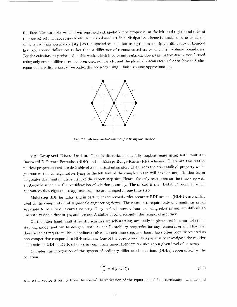
volume approach. Flow variables are stored at the vertices of the mesh, and control volumes are formed

by the median-dual graph of the original mesh, as shown in Figure 2.1. A control-volume flux balance is

computed by summing fuxes evaluated along the control volume faces, using the average values of the flow

variables on either side of the face in the flux computation. The construction of convective terms corresponds

to a second order accurate central difference scheme which requires additional dissipation terms for stability.

These may either be constructed explicitly as a blend of a Laplacian and biharmonic operators, or may be

obtained by writing the residual of a standard upwind scheme as the sum of a convective and dissit)ation

term:

1neighborsE 21 {F (wi) 4- F (Wk) } .nlk -- _ t Aik I (wL - Wa) (2.1)

k=l

where tile convective fluxes are denoted by F (w), nlk represents the normal vector of the control volume face

separating the neighboring vertices i and k, and Aik is the flux Jaeobian evaluated in the direction normal to

thisfilce.TilevariablesWLandWRret)resentextrapolatedflowpropertiesat theleft-andright-handsidesofthecontrolvohunefacerespectively.A matrix-basedartificialdissipationschemeisobtainedbyutilizingthesametransformationmatrix[Aik[ astheupwindscheme,but usingthisto multiplya differenceofblendedfirst andseconddifferencesratherthana differenceof reconstructedstatesat control-volume boundaries.

For the calculations performed in this work, which involve only subsonic flows, the matrix dissipation formed

using only second differences has been used exclusively, and the physical viscous terms for the Navier-Stokes

equations are discretized to second-order accuracy using a finite-volume approximation.

FIG. 2.1. Median control-volumes .for triangular meshes

2.2. Temporal Diseretization. Time is discretized in a fully implicit sense using both multistep

Backward Difference Formulas (BDF) and multistage Runge-Kutta (RK) schemes. There are two mathe-

matical properties that are desirable of a numerical integrator. The first is the "A-stability" property which

guarantees that all eigenvalues lying in the left, half of the complex plane will have an amplification fa(:tor

no greater than unity, independent of the chosen step size. Hence, the only restriction on the time step with

an A-stable scheme is the consideration of solution accuracy. The second is the "L-stable" property which

guarantees that eigenvalues approaching -oc are damped in one time step.

Multi-step BDF formulas, and in particular the second-order accurate BDF scheme (BDF2), are widely

used in the computation of large-scale engineering flows. These schemes require only one nonlinear set of

equations to be solved at each time step. They suffer, however, from not being self-starting, are difficult to

use with variable time steps, and are not A-stable beyond second-order temporal accuracy.

On the other hand, multistage RK schemes are self-starting, are easily implemented in a variable time-

stepping mode, and can be designed with A- and L- stability properties for any temporal order. However,

these schemes require multiple nonlinear solves at each time step, and hence have often been discounted as

non-competitive compared to BDF schemes. One of the objectives of this paper is to investigate the relative

efficiencies of BDF and RK schemes in computing time-dependent solutions to a given level of accuracy.

Consider the integration of the system of ordinary differential equations (ODEs) represented by the

equation,

dw

-- S (t,w(t)) (2.2)dt

where the vector S results from the spatial diseretization of the equations of fluid mechanics. The general

formula fi)r a k-step BDF scheme can be writt(m as:

k-1

Wn+ k = - E c_iw"+i + At3kSn+_" (2.3)

{--0

BDF schenms require the storage of k+l solution levels and the computation of one non-linear solution

at each time step. For k=2. the second-order accurate (BDF2) scheme is obtained using the coefficients:

at) = -4/3, O_ 1 : 1/3,/2 = 2/3. More details of these standard schemes can be found in [2, 5].

Runge-Kutta methods are inultistage schenies and at'(' implemented as:

± ()w {k} = w '_ + (At) ett.jS w tj} ,k=l,2 ..... s (2.4)

¢-1

w n+l = w n + (At) bjS w {j} (2.5)

j=t

where s is _he mmlber of stages arid aij and bj are the Butcher coefficients of the scheme. Following tile

previous work by Bijl et al. [2] we focus on the ESDIRK (:lass of RK schemes, which stands for Explicit

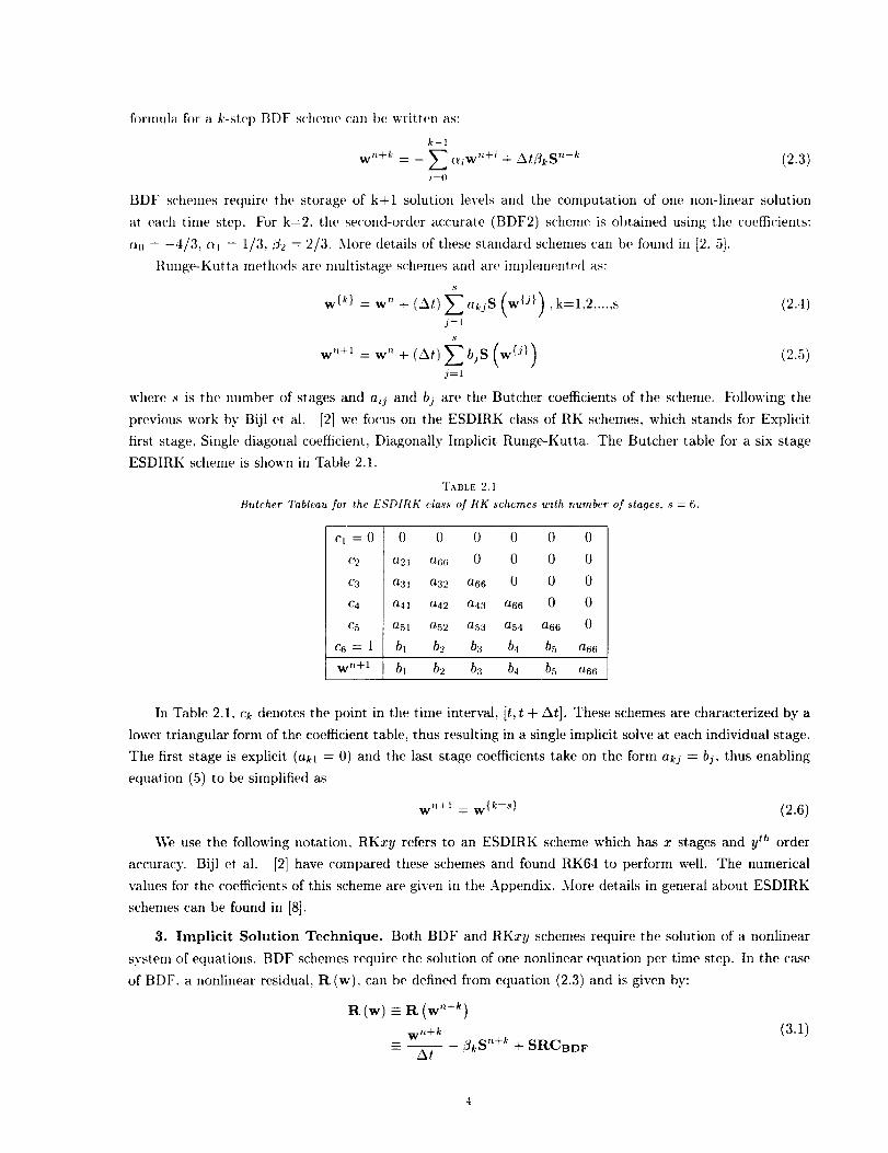
first stage, Single diagonal coefficient, Diagonally hnplicit Runge-Kutta. The Butcher table for a six stage

ESDIRK sehenle is shown in Table 2.1.

TABLE 2.1

Butcher Tableau for the ESDIRK class of RK schemes with number of stages, s = 6.

c, = (1 0 0 0 0 0 0

c2 a2_ a66 0 0 0 0

c3 a31 a32 a66 0 0 0

(:4 a41 a42 a43 a66 0 0

c5 a51 a52 a53 a54 a66 0

c6 = 1 bl b2 b3 b4 b5 a66

w n+l bl b2 b3 b4 b5 a66

In Table 2.1, ck denotes the point in the time interval, It, t + At]. These schemes are characterized by a

lower triangular form of the coefficient table, thus resulting in a single implicit solve at each individual stage.

The first stage is explicit (akl = 0) and the

equation (5) to be simplified as

last stage coefficients take on the form akj = bj, thus enabling

w '_+t = w {k=_} (2.6)

_,_,> use the following notation, RKxy re.fers to an ESDIRK scheme which has x stages and yth order

accuracy. Bijl et al. [2] have compared these schemes and found RK64 to perform well. Tile numerical

values fur the coefficients of this scheme are given in the Appendix. More details in general about ESDIRK

schemes can be found in [8].

3. Implicit Solution Technique. Both BDF and RKxy schemes require the solution of a nonlinear

system of equations. BDF schemes require the solution of one nonlinear equation per time step. In the case

of BDF, a nonlinear residual, R (w), can be defined from equation (2.3) and is given by:

R (w) _= U (w "+_)

wn+k (3.1)-- _kS n+k + SRCBDF- At

where the SUl)erscript on w has been dropt)ed for the sake of simt)licity. SRCBDF is the sonrce term

independent of w = w ''+t' and is given by,

SRCBDF _ _ I.i=00'wn+i (3.2)

In the case of RKxy schemes, a nonlinear systenl arises at each stage of t.}l(, time-stepping scheme and

hence more than one nonlinear solve per time step is required. Again, a nonlinear residual, R (w) for each

stage of the RK:ry scheme can t)e defined using equation (2.4) as follows:

R(w)- R(w {_'})

w{k} [ "_ (3.3)

- At akkSl, w{k}) + SRCRK

where tile superscript on w has again been dropped for the sake of simplicity. Also, SRCRK, is the source

term independent of w = w {k} and is given by,

k--I

W" (W{d})SRCRK _t E akj S (3.4)j=l

Hence, in both BDF and RKxy we are required to obtain the solution of the nonlinear system of

equations,

R(w) = 0 (3.5)

Three different nmthods are proposed for solving equation (3.5) and their relative t)erformances are

studied. The three nlethods, in this paper, are henceforth referred to as :

1. Nonlinear Multigrid (NMG)

2. Linear Multigrid (LMG)

3. Preconditioned Generalized Minimal Residual (PGMRES)

In NMG, a pseudo-time-stepping scheme is employed to obtain the solution of the nonlinear system of

equations, which is accelerated using a non-linear full approximation storage (FAS) agglomeration multigrid

method [11, 12]

In tim other two approaches, an inexact Newton solution strategy is used to solve the nonlinear system

of equations [14, 11, 15]. The resulting linear system of equations is solved using iterative/Krylov techniques.

To accelerate convergence, the linear system is left preconditioned using an approximate inverse to the first-

order accurate Jacobian which in itself is employed as an approximation to tile Jacobian of the second-order

accurate discretization. The last two approaches differ only in the methods used to solve tile preconditioned

linear system of equations. LMG uses the Riehardson's iterative method while PGMRES uses the Generalized

Minimal Residual method developed by Yaad and Schultz [16].

3.1. NonLinear Multigrid (NMG). In a pseudo-time stepping scheme, the e(tuations are integrated

in pseudo-time until Eq. (3.5) is satisfied.

dw-- + a(w) = 0 (3.6)dr*

where t* is tile t)seudo-time. Since we do not require a pseudo-time accurate solution, the equations are

preconditioned to accelerate the convergence. Hence, we have,

p_, dw37 + a(w) = 0 (3.r)

Tile equations are integrated in pseudo-time using an explicit preconditioned multi-stage schenm [10],

which can he written as :

w (°) = w [k]

w(l: = w(°) _ At*PR (w(°))

w(q) = w(q-1) - 2__,*PR (w(q-1) )

w[_'+ 1] = w(q)

(3.s)

fl)r a q-stage scheme.

An agglomeration multigrid strategy previously developed as a solver for steady-state problems [10] is

used to flzrther accelerate convergence. The agglomeration multigrid may be viewed as a simplified algebraic

multigrid strategy. Coarse level grids are constructed by fusing together or agglomerating neighbouring con-

trol volumes t.o form a coarser set of larger lint more complex control volumes. In the algebraic interpretation

of agglomeration nmltigrid, the coarse levels are no longer geometric grids, but represent groupings of fine

grid equations which are summed together to form the coarse grid equations sets [9, 6] The basic smoother on

each grid level is a three-stage explicit preconditioned multi-stage scheme with stage coefficients optimized

for high frequency damping properties [11.

The preconditioner, P is chosen to be the block diagonal of the Jacobian of the residual, R (w),

__p_l = Dii k-O-_wiJ,,,o, (3.9)

This isreferredto as Jacobi preconditioningand providessubstantialincreasesinefficiencywhen upwind or

matrix dissipationdiscretizationsare used [18].Itshould be noted that the use of Jacobi preconditioning

involvesinvertinga 4 x 4 matrix foreach vertexat each stage.

3.2. Inexact Newton's Methods. To solvethe non-linearsystem ofequations R (w) = 0,Newton's

method requiresthe solutionofa seriesoflinearsystems ofthe form,

where,

w[k+ 1] = w [k}+ 5w [k]

(3.10)

(3.11)

Let,

x -- 5w[_'];

Hence. equation (3.10) now becomes,

( )r = R w [k] ," A - (3.12)

Ax = -r (3.13)

Traditionally, there have been two main obstacles to the use of Newton's method fl)r large-scale multi-

physics applications :

1. An initial guess inside o/the radius of convergence is required for Newton's method to converge.

However, for unsteady problems, a good initial guess is provided by the solution at the previous

time step.' If the Newton's method does not converge, then by lowering the time step one can get

the initial guess as (:lose as necessary to the solution at the next time level. In the calculations

presented in this paper, no difficulties were encountered in the convergence of the Newton iterations

for an5' of the time steps used.

2. ConstructioTt and storage of the Jacobian matrix, A becomes prohibitive. This prohlen_ is particularly

exacerbated in 3D for higher-order spatial discretizations which are not confined to the nearest

neighbor stencils. This problem is overcome by the use of Jacobian-free methods to solve the linear

system of equations. However, additional memory is still required to store the first-order Jacobian

for the preconditioning operation, and the various Krylov vectors for the GMRES scheme. On the

other hand, the use of additional memory can be rationalized if this produces substantial gains in

CPU time, particularly for unsteady flow simulations where epu tiIne is the dominant ('oncern.

Additionally, in order to improve the computational efficiency of these methods, we use an inexact Newton's

method[14, 3] where the arising system of equations are not solved exactly. In this paper, we emt)loy a very

simplistic inethod where the number of iterations carried out by the underlying iterative linear solver is held

fixed. In it's exact form, Newton's method provides quadratic convergence. However due to the various

approximations employed by the sohltion method in this paper, this rate of convergence is not achieved.

3.3. Preconditioned Inexact Newton's Method. In order to achieve rapid convergence of the

linear problem at each Newton iteration, preconditioning methods are used to cluster the eigenvalues of the

system. We adopt the approach of left preconditioning in order to achieve this desirable distrilmtion of

eigenvalues. The preconditioned system can be written as:

"P_:'Ax = -P_,r (3.14)

We make the following comments on the preconditioning:

• The preconditioner, T'._', is looked upon here as an operator as opposed to a matrix. Hence, P_,,

may or may not be able to be written as a matrix.

• The preconditioner must be chosen as close as possible to A -1 so that T'_A _ Z, where 2" is the

identity operator.

• Since each step of the Newton's method, equation (3.10), moves w [k}, towards the solution, w*, of

R (w) = 0, any operator which produces a correction 6w [kl = x to advance w [_'l towards w" would

serve as a reasonable preeonditioner.

• Based on the above fact, single or muhiple cycles of the nonlinear multigrid method discussed in the

earlier subsection could be used as a preconditioner. However, this is eomputationally inefficient as

it does not recognize the fact that we are now solving a system of linear equations.

Keeping in mind the above observations we now propose a better preconditioner, P,_,. We first choose

,p._, = _-l, where P, is a matrix approximation to the Jacobian, A. Considerations governing the choice of

would be,

1. Storage requirements for A must not be prohibitive. Storage for A nmst use less space than that

needed for A or else there would be no space gain in using Jaeobian-free methods.

2. The inverse era m.ust be simple to calculate or approximate. If one is able to compute an approximate

inverse to A fairly easily using iterative methods, this new operator, 7_N = .A would serve as

all apt)rot)riatepreconditioner.Tile twotildesareusedto symbolizethefactthat tiler(,aretwoapproximationsinvolvedill thedefinitionof tile T'A';

(a) A which is all approxinlation to the Jacobian, A

(b) An approxintation in computing the inverse of

In this paper, we choose A to be the Jacohian of the first-order accurate, nearest neighbor discretization of

the nonlinear set of equations. Hence, the storage of _, requires substantially less memory than that of the

fifll Jacobian A of the second-order accurate scheme.

_-1 is computed approximately using a fixed number of W-cycles of a linear multigrid method. This

particular nmltigrid method Call be viewed as the linear analogue of the non-linear FAS agglomeration

multigrid scheme described in the NMG method. This approach has been previously described in detail

in reference [12]. In this particular approach the coarse level approximations to the Jm:obian are obtained

taking the Jacobian of the Galerkin projection of the (frozen) fine grid operator as:

0

AH = Ow,----7(IHRhI_)

as opposed to the more traditional linear multigrid Galerkin projection:

H 0Ra h = iHAhlhHAN = Ih 0---"_H IH

(3.15)

(3.16)

where I_ is the restriction operator and I_ is the prolongation operator. This approach was chosen purely

for convenience, as the terms in equation (3.15) are readily available. The smoother on each grid was taken

as a block diagonal 3acobi solver.

3.4. Linear Multigrid (LMG). In the method referred to as LMG, the linear muhigrid precondi-

tioned system arising at each Newton iteration is solved using a single Richardson iteration, hi order to

solve the system,

we define the splitting [4]

PA'Ax = -T'A'r (3.17)

P_,A = Z + A _ (3.18)

The resulting iterative scheme is defined as.

Zx (,,, + 1) = _ P, vr - ,_'x (rn )

Z_x (m) = -PA'r - P_'hx (m) (3.19)

As indicated earlier, since we are required to solve equation (3.17) only approximately, we carry out only a

single Richardson's iteration. Assuming x (ll = 0, equation (3.19) reduces to,

6x (1) = -P,_,,r (3.20)x (2) = x (t) + 6x (_) = 5x (_) = -PAw

Hence, we have

3w[*q = x (2) = -T%'r (3.21)

Equation (3.21) illustrates the correspondence of this scheme to a Newton's method in which the first-order

accurate Jacot)ian is used along with a second-order accurate residual.

3.5. PreconditionedGeneralized Minimal Residual (PGMRES). Having presented th(' LMG

scheme as a precondition('d Richardson iteration, the PGMRES scheme can similarly be described as th('

equivalent schente obtained when the single Richardson iteration is replaced by a GMRES Krvlov subsi)ace

iterative at)proach [17]. In this method, we use GMRES to solve equation (3.14) in a matrix-free Newton-

Krylov fashion [20], making use of the same preconditioner, P,,,,, which is used in the linear multigrid method

(LMG). The matrix-free implementation of PGMRES requires th(, computation of the t)roduct. _Ax, which

is approximated using a first-order Taylor series expansion as,

(will+ - (wlkl)7'_,Ax =

e (3.22)/)._,R (w !k] + _x) - _,_r

where x is some unit vector and _ is a number chosen close to machine round-off. We use the restarted

form of GMRES with a fixed number of search directions. While increasing ttw number of Kryh)v vectors

accelerates convergence, storage and cpu time increase with the number of search directions. The Ol)timal

number of search directions is therefore determined experimentally.

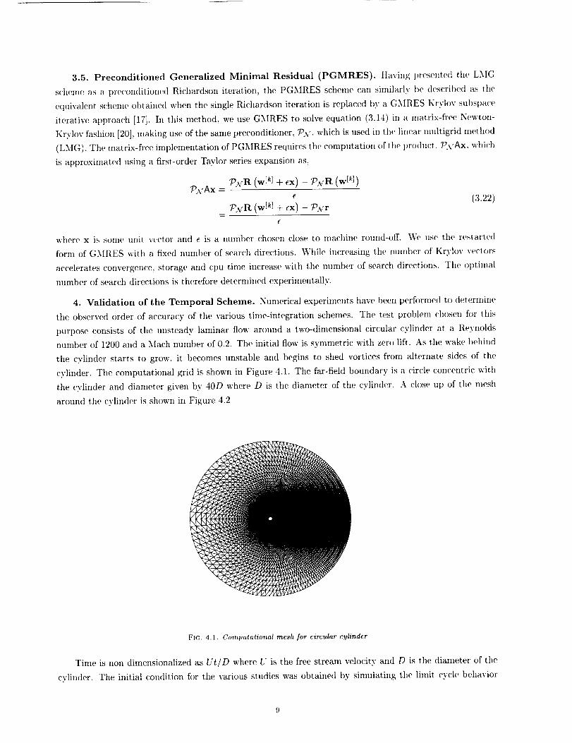
4. Validation of the Temporal Scheme. Numerical experiments have been performed to (tetermine

the observed order of accuracy of the various time-integration schemes. The test problem chosen for this

purpose consists of the unsteady laminar flow around a two-dimensional circular cylinder at a Reynolds

nmnber of 1200 and a Mach number of 0.2. The initial flow is symmetric with zero lift. As the wake behind

the cylinder starts to grow, it becomes unstable and begins to shed vortices from alternate sides of the

cylinder. The computational grid is shown in Figure 4.1. The far-field boundary is a circle concentric with

the cylinder and diameter given by 40D where D is the diameter of the cylinder. A close ut) of the mesh

around the cylinder is shown in Figure 4.2

FIG. 4.1. Computational mesh for circular cylinder

Time is non dimensionalized as Ut/D where U is the free stream velocity and D is the diameter of the

cylinder. The initial condition for the various studies was obtained by simulating the limit cycle behavior

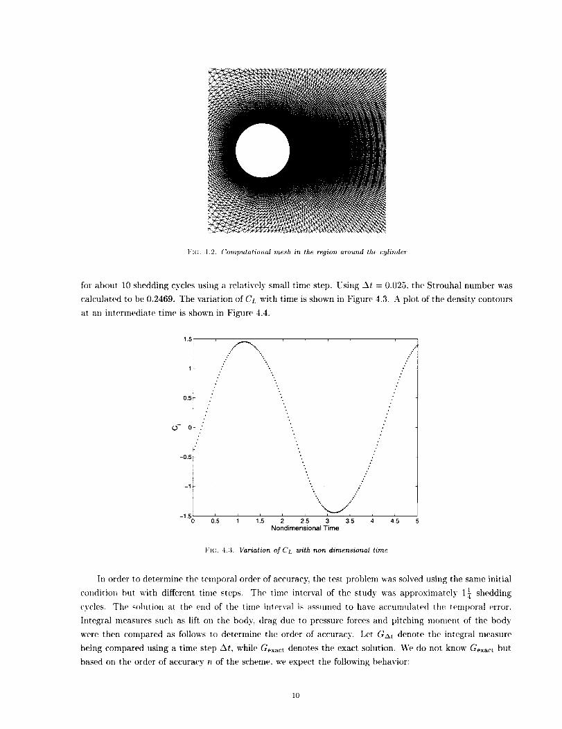
t:I(:. 4,2. (:omputational mesh in the region around thr cylinder

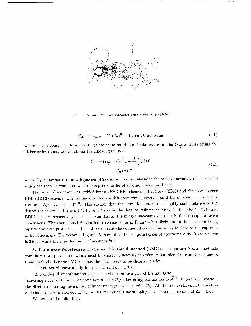
for about 10 shedding cycles using a relatively small time step. Using At = 0.025, the Strouhal number was

calculated to be 0.2469. The variation of CL with time is shown in Figure 4.3. A plot of the density contours

at an intermediate time is shown in Figure 4.4.

-1

Nondimensional Time

t",c:. 4.3. Variation of CL with non dimensional time

In order to determine the temporal order of accuracy, the test problem was solved using the same initial

condition but with different time steps. The time interval of the study was approximately 1_ shedding

cycles. The solution at the end of the time interval is assumed to have accunmlated the temt)oral error.

Integral measures such as lift on the body, drag due to pressure forces and pitching moment of the body

were then (:ompared as follows to determine the order of accuracy. Let GAt denote the integral measure

being compared using a time step At, while Go .... t denotes the exact solution. We do not know G_t but

based on the order of accuracy n of the scheme, we expect the following behavior:

10

/

(

4L/

FIG. 4.4. I)ensity Contours calculaled using a lime step of 0.025

G,,t = Gexact + C1 (At) '* + Higher Order Terms (4.1)

where Cl is a constant. By subtracting from equation (4.1) a similar expression for G .,__ and neglecting the

higher-order terms, we can obtain the following relation,

G_t-G_ =C' (l + _--_') (At)'_ (4.2)

= C2 (_t)"

where C2 is another constant. Equation (4.2) can be used to determine the order of accuracy of the scheme

which can then be compared with the expected order of accuracy based on theory.

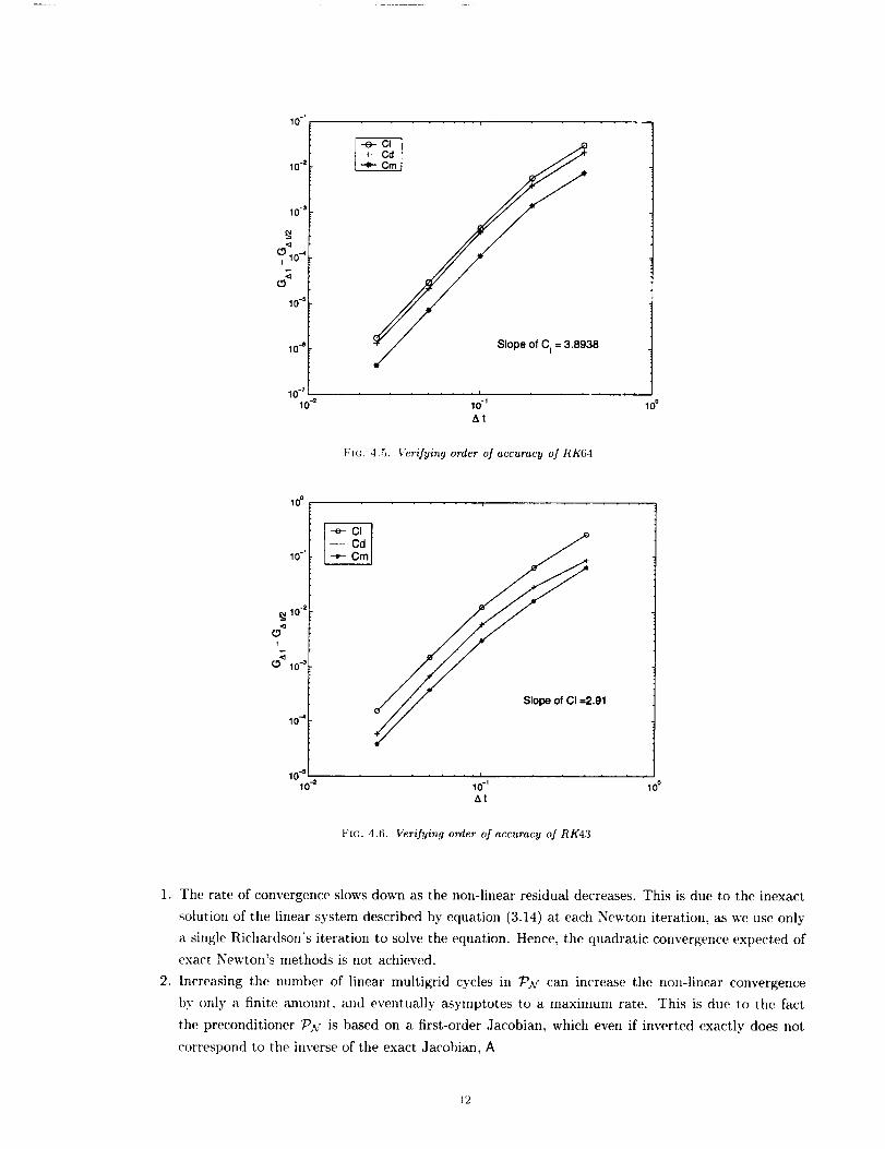
The order of accuracy was verified for two ESDIRK schemes ( RK64 and RK43) and the second-order

BDF (BDF2) scheme. The mmlinear systems which arose were converged until the maximum density cor-

rection, [Ap [..... < 10 -m. This ensures that the "iteration error" is negligibly small relative to the

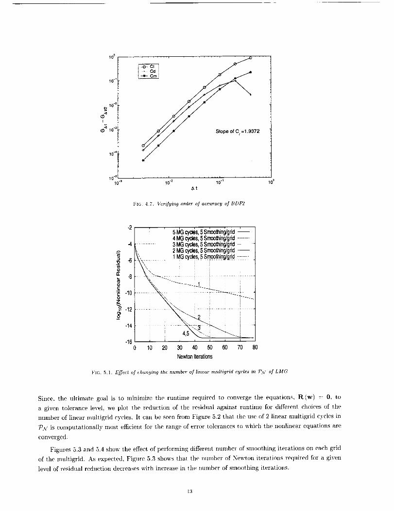
discretization error. Figures 4.5, 4.6 and 4.7 show the detailed refinement study for the RK64, RK43 and

BDF2 schemes respectively. It can be seen that all the integral measures yield nearly the same quantitative

conclusions. The anomalous behavior for large time steps in Figure 4.7 is likely due to the timesteps being

outside the asymptotic range. It is also seen that the computed order of accuracy is close to the expected

order of accuracy. For example, Figure 4.5 shows that the computed order of accuracy for the RK64 scheme

is 3.8938 while tile expected order of accuracy is 4.

5. Parameter Selection in the Linear Multigrid method (LMG) . The inexact Newton methods

contain various parameters which must be chosen judiciously in order to optimize the overall run-time of

these methods. For the LMG scheme, the parameters to be chosen include:

1. Number of linear rnultigrid cycles carried out in _"

2. Number of smoothing iterations carried out on each grid of the multigrid.

Increasing either of these parameters would make _" a better approximation to _-1. Figure 5.1 illustrates

the effect of increasing the number of lineal" multigrid cycles used in _'. All the results shown in this section

and the next are carried out using the BDF2 physical time stepping scheme and a timestep of At = 0.05.

We observe the following :

11

10 -1

10-=

10 -3

<]

10 "4

10 -s

10 4

10 -7

10 -=

= , 8

, , , , , i i i , , ,

10-1

At

FIG. 4.5. Verifying order of accuracy of RK64

100

10 o

10 -_

10-=

r3t

C_< lO-3

10--4

1o -= 10 °

.91

, i t , , . , , ,

10 -I

At

FIG. 4.6. Verifying order of accuracy of RK43

1. The rate of convergence slows down as the non-linear residual decreases. This is due to the inexact

solution of the linear system described by equation (3.14) at each Newton iteration, as we use only

a single Richardson's iteration to solve the equation. Hence, the quadratic convergence expected of

exact Newton's methods is not achieved.

2. Increasing the number of linear multigrid cycles in T'A," can increase tile non-linear convergence

by only a finite amount, and eventually asymptotes to a maximum rate. This is due to the fact

the preconditioner P_, is based on a first-order Jacobian, which even if inverted exactly does not

correspond to the inverse of the exact Jacobian, A

12

100

10 -1

10 .2

I

(_104

10 .4

, i ...... !

72

10 -5 , , , ,,,I , , _,,I

10 -a 10°2 10 -1

At

FIG. 4.7. Verifying order of accuracy of BDf_2

100

-2 ' 5 MGcycles,5 Smoothing/grid'4 MGcycles,5 Smoothing/grid..........

-4 ;.................I...... 3 MGcycles,5 Smoothing/grid............_,.. 2 MGcycles,5 Smoothing/grid--

i1 .................._ .......i..........i-J.......2._ i

-I0 _,_ i : "-"_............

Z ; '_ i J

__ -12.14...........i.... i _..... !; .........i ..............-_ .............:..... ! ........

4,5_ .......i.,, "_-16 i i i i i i i

0 10 20 30 40 50 60 70 80

NewtonIterations

FIG. 5.l. Effect of changing the number of linear multigrid cycles in 7_," of LMG

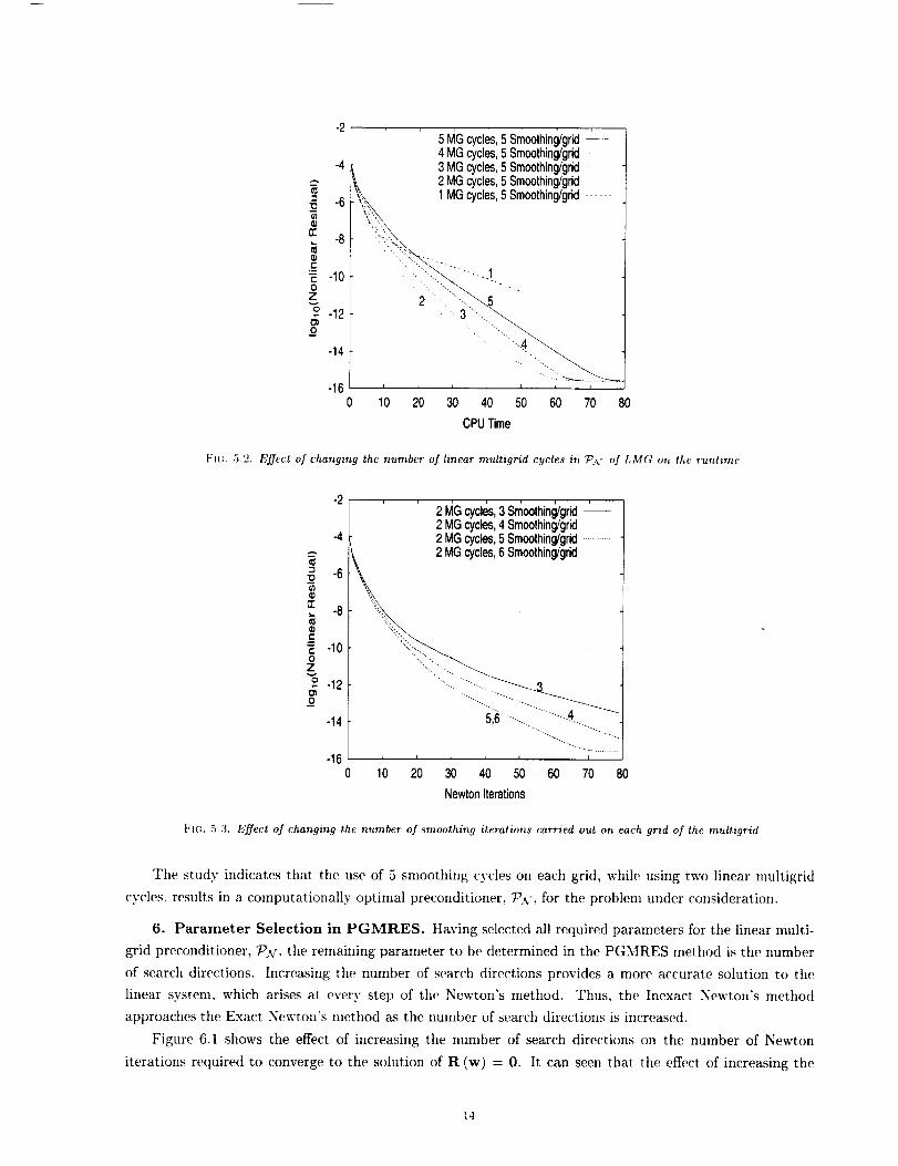
Since, the ultimate goal is to minimize the runtime required to converge the equations, R(w) = O, to

a given tolerance level, we plot the reduction of tim residual against runtime for different choices of the

number of linear inultigrid cycles. It can be seen from Figure 5.2 that the use of 2 linear multigrid cycles in

;aA_ is computationally most efficient for the range of error tolerances to which the nonlinear equations are

converged.

Figures 5.3 and 5.4 show the effect of performing different number of smoothing iterations on each grid

of the multigrid. As expected, Figure 5.3 shows that the number of Newton iterations required for a given

level of residual reduction decreases with increase in the number of smoothing iterations.

13

q)0a

rr

¢-Dt-O

zv

_o

-2

-4

-6

-8

-10

-12

-14

-160

' ' 5 I_Gcycles,5 Snloothing/grid '4 MGcycles,5 Smoothing/grid3 MGcycles,5 Smoothing/grid-2 MGcycles,5 Smoothing/grid

i!_ 1 MGcycles,5 Smoothing/grid------_

•iLl,...!............12"' ..... 5 ....

i! 3"'"',.

I t I I I I

10 20 30 40 50 60 70 80

CPUTime

FIG 52. Effect of changing the number of linear mutt=grid cycles in g',,( of LM(; on the runtime

.2

-4

"_ -6q)

tv-8

e-

_- -10O

z9 -12

_o

-14

-16

' 2 I_Gcycles,3 Smoothing/grid--2 MGcycles,4 Smoothing/grid2 MGcycles,5 Smoothing/grid2 MGcycles,6 Smoothing/grid

5 6......... "........

I 1 I I I I I

10 20 30 40 50 60 70 80

NewtonIterations

FI(:, 5.3. Effect of changing the number of smoothing iterations carried out on each grid of the multigrid

The study indicates that the use of 5 smoothing cycles on each grid, while using two linear multigrid

cycles, results in a computationally optimal preconditioner, 5PN, for the problem under consideration.

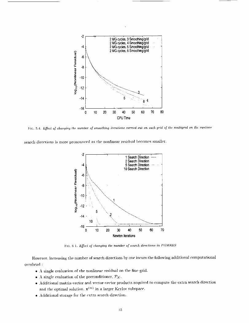
6. Parameter Selection in PGMRES. Having selected all required parameters for the linear multi-

grid preconditioner, 5ov, the remaining parameter to he determined in the PGMRES method is the mlmber

of search directions. Increasing the number of search directions provides a more accurate solution to the

linear system, which arises at every step of the Newton's method. Thus, the Inexact Newton's method

approaches the Exact Newton's method as the number of search directions is increased.

Figure 6.1 shows the effect of increasing the number of search directions on the number of Newton

iterations required to converge to the solution of R (w) = 0. It can seen that the effect of increasing the

14

t_

rr

c-

Oz

o

-2 , 2 MGcycles,3 Sn_oothing/grid--2 MGcycles,4 Smoothing/grid

-4 2 MGcycles,5 Smoothing/grid......2 MGcycles,6 Smoothing/grid

-8

-10

42 t " i!'i'_-t4 ...........i_---4

-16 ! ' ' ' ' ' ' '0 10 20 30 40 50 60 70

CPUTime

80

FIG. 5+4. Effect o/changing the number o/ smoothing iterations carried out on each grid o/the multigrid on the runtime

search directions is more pronounced as the nonlinear residual becomes smaller.

-2 ' ' ' 1,£earchDirection'2 SearchDirection

-4 5 SearchDirection......

i"8"__^I__c -6 10SearchDirection

-10

_o 5 "",",2

-12

-14

-160

i i i i i i

10 20 30 40 50 60 70

NewtonIterations

F1G. 6 I. Effect o.f changing the number o/ search directions in PGMRES

However, increasing the number of search directions by one incurs the following additional computational

overhead :

• A single evaluation of the nonlinear residual on the fine grid.

• A single evaluation of the preconditioner, 7)_ ".

• Additional matrix-vector and vector-vector products required to compute the extra search direction

and the optimal solution, x ('_/ in a larger Krylov subspace.

• Additional storage for the extra search direction.

15

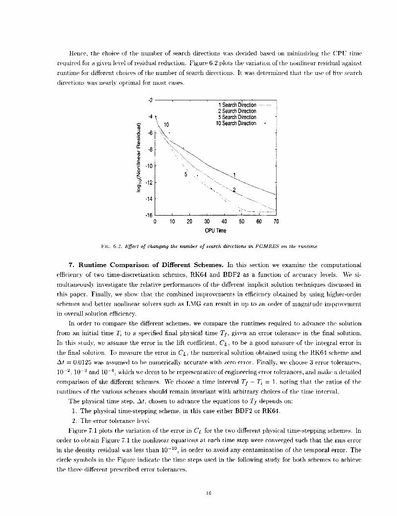
Hence,thechoiceof thenumberof searchdirectionswasdecidedbasedonmininlizingtheCPUtimerequiredforagivenlevelofresidualreduction.Figure6.2plotsthevariationofthenonlinearresidualagainstruntimefl)rdifferentchoices of the number of search directions. It was determitmd that the use of five search

directions was nearly optimal for most cases.

¢}

e-

t-0

zO

_o

-2

-4

-6

-8

-10

-12

-14

-16 I0

' ' ' 1 _arch Direction'2 SearchDirection

lI1

L L i I I _--1

10 20 30 40 50 60 70

CPUTime

FIG. 6.2. Effect of changing the number of search directions in PGMRES on the. runtime

7. Runtlme Comparison of Different Schemes. In this section we examine the computational

efficiency of two time-discretization schemes, RK64 and BDF2 as a function of accuracy levels. We si-

multaneously investigate the relative performances of the different implicit solution techniques discussed in

this paper. Finally, we show that the combined improvements in efficiency obtained by using higher-order

schemes and better nonlinear solvers such as LMG can result in up to an order of magnitude improvement

in overall solution efficiency.

In order to compare the different schemes, we compare the runtimes required to advance the solution

from an initial time 7", to a specified final physical time TI, given an error tolerance in the final solution.

In this study, we assume the error in the lift coefficient, CL, to be a good measure of the integral error in

the final solution. To measure the error in CL, tile numerical solution obtained using the RK64 scheme and

At = 0.0125 was assumed to be numerically accurate with zero error. Finally, we choose 3 error tolerances,

10 -2, 10 .3 and 10 -4, which we deem to be representative of engineering error tolerances, and make a detailed

comparison of the different schemes. We choose a time interval 7"/ - 7", = 1, noting that the ratios of tile

runtimes of the various schemes should remain invariant with arbitrary choices of the time interval.

The physical time step, At, chosen to advance the equations to T/ depends on:

1. The physical time-stepping scheme, in this case either BDF2 or RK64.

2. The error tolerance level

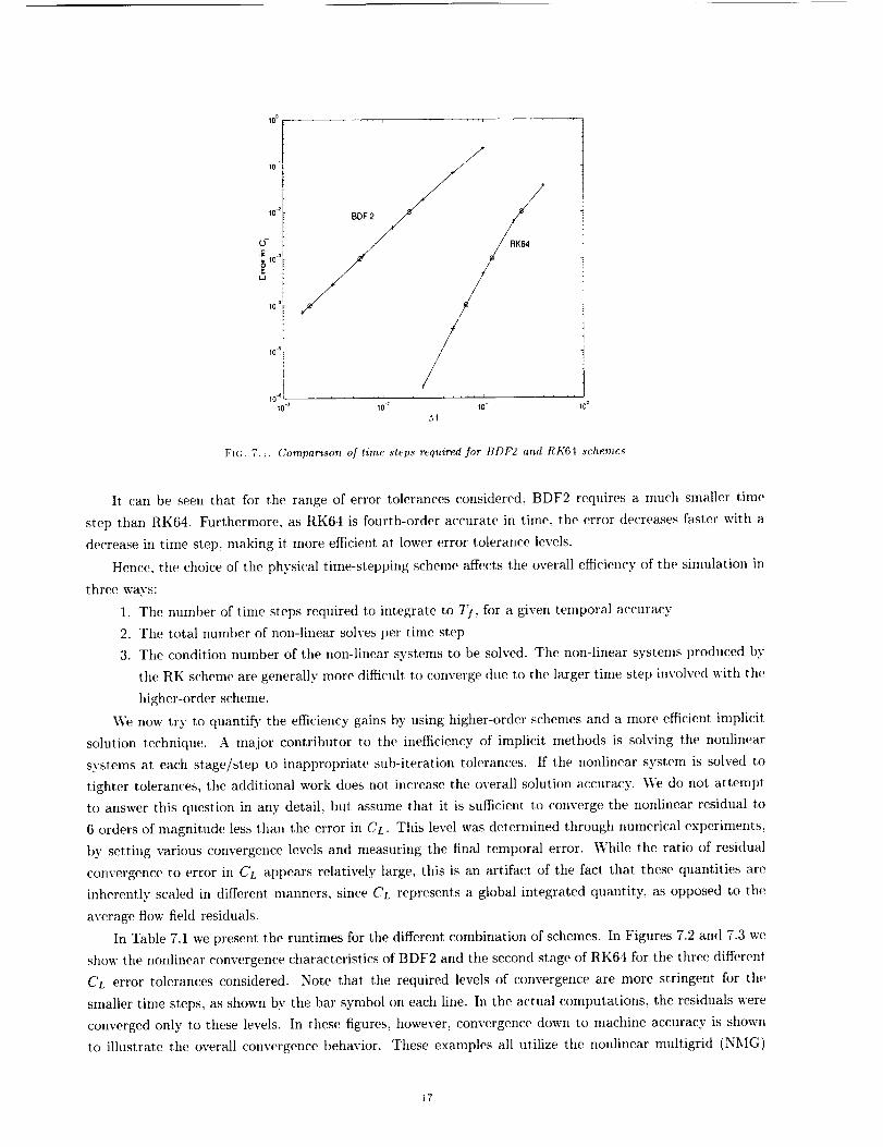
Figure 7.1 plots the variation of the error in CL for the two different physical time-stepping schemes. In

order to obtain Figure 7.1 the nonlinear equations at each time step were converged such that the rms error

in the density residual was less than 10 -1°, in order to avoid any contamination of the temporal error. The

circle symbols in the Figure indicate the time steps used in the following study for both schemes to achieve

the three different prescribed error tolerances.

16

10 D

10 _

o-"E 10_

w

10 5

10

_0-_ 10_

BOF' /

, , , , , ,,,j , , ,,,i

10-; 1(]-_

5t

FIG. 7.1. Comparison of time steps required for BDP2 arm RK64 schemes

It. (:an be seen that for the range of error tolerances considered, BDF2 requires a much smaller time

step than RK64. Furthermore, as RK64 is fourth-order accurate in time, the error decreases faster with a

decrease in time step, making it more efficient at lower error tolerance levels.

Hence, the choice of tile physical time-stepping scheme affects the overall efficiency of the simulation in

three ways:

1. The number of time steps required t.o integrate to Tf, for a given temporal accuracy

2. The total number of non-linear solves per time step

3. The condition number of the non-linear systems to be solved. The non-linear systems produced by

the RK scheme are generally more difficult t.o converge due to the larger time step inw)lved with the

higher-order scheme.

\_ now try to quantify the efficiency gains by using higher-order schemes and a more efficient implicit

solution technique. A major contributor to the inefficiency of implicit methods is solving the nonlinear

systems at each stage/step to inappropriate sub-iteration tolerances. If the nonlinear system is solved t.o

tighter tolerances, the additional work does not increase the overall solution accuracy. We do not att.empt

to answer this question in any detail, but assume that it is sufficient to converge the nonlinear residual to

6 orders of magnitude less than the error in Ca. This level was determined through numerical experiments,

by setting various convergence levels and measuring the final temporal error. While the ratio of residual

convergence to error in CL appears relatively large, this is an artifact, of the fact that these quantities are

inherently scaled in different manners, since CL represents a global integrated quantity, as opposed t.o the

average flow field residuals.

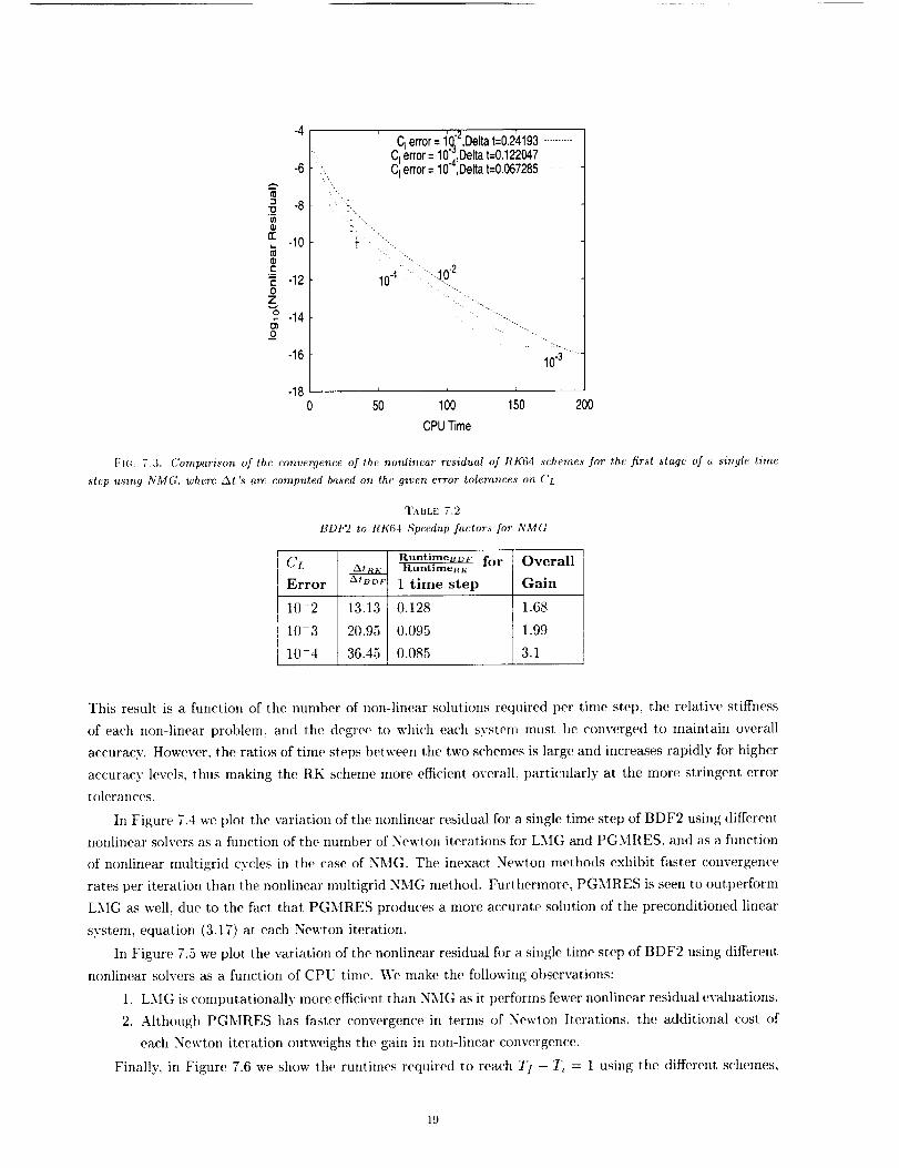
In Table 7.1 we present the runtimes for the different combination of schemes. In Figures 7.2 and 7.3 we

show the nonlinear convergence characteristics of BDF2 and the second stage of RK64 for the three different

CL error tolerances considered. Note that the required levels of convergence are more stringent for the

smaller time steps, as shown by the bar symbol on each line. In the actual computations, the residuals were

converged only to these levels. In these figures, however, convergence down to machine accuracy is shown

to illustrate the overall conw_rgence behavior. These examples all utilize the nonlinear nmltigrid (NMG)

17

TABLE 7. l

Runtimes (in seconds on l'cntium I V, 1700MIIZ) required for earr'ying out l physical lime ,step using the different nonlinear

solvers, where time sleps are chosen based on the given errvr tolerances on CL

Scheme At NMG

CL Error =

BDF 0.01842 15.55

RK 0.24193 121.56

CL Error=

BDF 0.005825 12.45

RK 0.122047 131.4

CL Error =

BDF 0.001846 12.49

RK 0.067285 147.14

LMG PGMRES

10-2

5.24 9.00

39.52

10-:t

4.59 9.01

43.84

10-,I

5.54 8.76

44.91

schoule.

-2

.64Ii!

._CCcm'_ -8 !-10

Z

o -12t__o

-14

-160

' GI error= 1Q;2,Deltai=0.01842 'C=error= lO",Deltat=0.005825

CIerror= lO4,Deltat = 0.001846

10-4 t0.3-_., ..... 10.2

..... "?!:211

I I I t I t I

20 40 60 80 100 120 140

CPUTime

Fla. 7.2. Comparison of the convergence of the nonlinear residual of BDF2 schemes for a single time step using NMG,

where At's are computed based on the given error tolerances on CL

We observe the following :

1. Faster convergence for smaller error tolerances, as At is reduced.

2. Slower overall convergence for RK64 relative to BDF2 h)r sinfilar error tolerances, as larger time

steps are used in RK64.

3. Although not shown, similar behavior is observed for the other two methods (LMG, PGMRES) as

well.

In Tables 7.2 and 7.3 we quantify the efficiency gains obtained by shifting from BDF2 to RK64 for the

two different nonlinear solvers, NMG and LMG respectively. The numbers in the different columns are ratios

of the corresponding quantities used in RK and BDF respectively. The CPU time for a given time step is

an order of magnitude larger for the RK schemes, and this ratio varies slowly with the increase in accuracy.

18

-4

-6

"_ -8

to

n" -10

@r"

c -12Oz

-14

_o

-16

' 2

CIerror= 1_ ,Deltat=0.24193..........CI error= 10"_,Deltat=0.122047CI error= 104,Deltat=0.067285

.L "'-,

10.4 iii"..]02

10.3 .....

-18 ' ' '0 5O 100 150 2O0

CPUTime

F,(;. 7.3. Comparison of lhc convergence of the nonlinear residual of RK6.1 schemes for the first stage of a single time

step _lsing NMG. where At's are computed based on the given error" tolerances on CL

TABLE 7.2

BDb'2 to RK64 ,qpeedup factors for NMG

CLError AIBDFi

10-2 13.13

1(}-3 20.95

10-4 36.45

RuntimeBDF forRuntimenK

1 time step

0.128

0.095

0.085

Overall

Gain

1.68

1.99

3.1

This result is a flmction of the number of non-linear solutions required per time step, the relative stiffness

of each non-linear problem, and the degree to which each system must be converged to maintain overall

accuracy. However, the ratios of time steps between the two schemes is large and increases rapidly for higher

accuracy levels, thus making the IlK scheme more efficient overall, particularly at the more stringent, error

tolerances.

In Figure 7.4 we plot the variation of the nonlinear residual for a single time step of BDF2 using different

nonlinear solvers as a flmction of the number of Newton iterations for LMG and PGMRES, and as a function

of nonlinear nmltigrid cycles in the case of NMG. The inexact Newton methods exhibit faster convergence

rates per iteration than the nonlinear inultigrid NMG method. Furthermore, PGMRES is seen to outperform

LMG as well, due to the fact that PGMRES produces a more accurate solution of the preconditioned linear

system, equation (3.17) at each Newton iteration.

In Figure 7.5 we plot the variation of the nonlinear residual for a single time step of BDF2 using different

nonlinear solvers as a function of CPU time. We make the following observations:

1. LMG is computationally more efficient than NMG as it performs fewer nonlinear residual evaluations.

2. Although PGMRES has faster convergence in terms of Newton Iterations, the additional cost of

each Newton iteration outweighs the gain in non-linear convergence.

Finally, in Figure 7.6 we show the runtimes required to reach Tf - Ti = 1 using the different schemes,

19

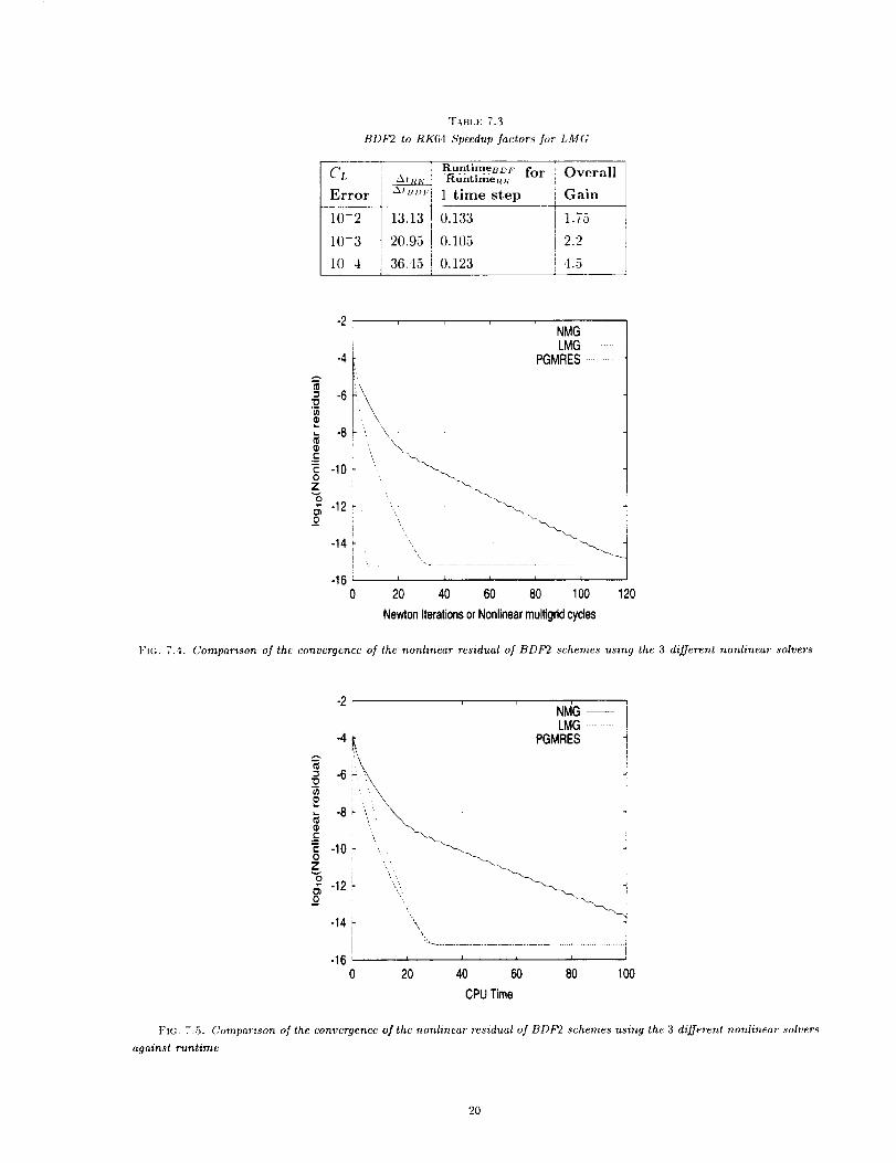
"I'ABLE7.3BDF2 to RK64 Speedup factors for LMG

Error

10-2

111-3

10 4

13.13

20.95

36.45

RuntimeBpF forRuntimeRh'

1 time step

0.133

0.105

0.123

Overall

Gain

1.75

2.2

4.5

t_

.¢

¢-B¢-Oz

o

5_o

-2

-4

-6

-8

-10

-12

-14

-16 [0

qNMG --LMG

PGMRES

\

i i i i i

20 40 60 80 100 120

NewtonIterationsor Nonlinearmultigridcycles

FIG. 7..t. Comparison of the convergencc of the nonlinear residual of BDF'2 schemes using the 3 different nonlinear solvers

-i.v

z_¢-0z

o

o_

-2

-4

-6

-8

-10

-12

-14

-16

NM'G--LMG

PGMRES .......

\

I I I I

20 40 60 80 100

CPUTime

I:'I¢3. 7.5. Comparison of the convergence of the nonlinear residual of BDF2 schemes using the 3 different nonlinear solvers

against runtime

20

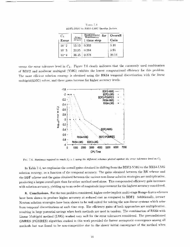
+['.,'d+LF, 7+1

BDf+_2-NMG to f+K61-LMG Speedup factors

CLError _t++tJF

10-2 13.13

10-3 20.95

10-4 36.45

Runtime_D+- forRuntlmet+K

1 time step

0.393

0.284

0.278

Overall

Gain

5.16

5.95

10.14

versus the error tolerance level in CL. Figure 7.6 clearly indicates that the c()mmonly used combination

of BDF2 and nonlinear multigrid (NMG) exhibits the lowest computational efficiency for this problem.

The most efficient solution strategy is obtained using the RK64 temporal discretization with the linear

multigrid(LMG) solver, and these gains increase for higher accuracy levels.

-1.8

-2

-2.2

-2.4

(J -2.6{::

-2.8W -3

O

-3.2_o

-3.4

-3.6

-3.8

-40

' ' BDF2NMG '

• ,_ BDF2-LMG

,_ \ BDF2-PGMRES ,RK64-NMGRK64-LMG......

, , \\

, ', \

1000 2000 3000 4000 5000 6000 7000

CPUTime

Ftc, 7.6. Runtimes required to reach Tf = 1 using the different schemes plotted against the error tolerance level in CL

In Table 7.4, we emphasize the overall gains obtained in shifting from the BDF2-NMG to the RK64-LMG

solution strategy, as a fimction of the temporal accuracy. The gains obtained between the RK scheme and

the BDF scheme and the gains obtained between the various non-linear solution strategies are multiplicative,

producing a larger overall gain than for either method used alone. This compounded efficiency gain increases

with solution accuracy, yielding up to an order of magnitude improvement for the highest accuracy considered.

8. Conelusions. For the test problem considered, higher-order implicit multi-stage Runge-Kutta schemes

have been shown to produce higher accuracy at reduced cost as compared to BDF2. Additionally, inexact

Newton solution strategies have been shown to be well suited for solving the non-linear systems which arise

from temporal diseretizations at each time step. The efficiency gains of both approaches are multiplicative,

resulting in large potential savings when both methods are used in tandem. The combination of RK64 with

Linear Multigrid method (LMG) worked very well for the error tolerances considered. The preconditioned

GMRES (PGMRES) algorithm studied in this work provided the fastest asymptotic convergence among all

methods but was found to be non-competitive due to the slower initial convergence of the method when

21

only partial convergence of the linear systems is required. In cases where more accurate linear system solu-

tions are required, PGMRES may be more competitive. Overall efficiency of the time-integration scheill(_S is

greatly affected by the degree to which the non-linear systems at each time step arc converged. The levels

of convergence adopted in this work were determined a posteriori, and are therefore not predictive. A more

exact quantification of the required convergence levels will be required in order to construct eIlicieltt tinle-

dependent solution strategies.Future work will also include the use of temporal error estinmtion techniques

coupled with dynanfically adaptive time-step selection.

Acknowledgments. The authors would like to thank the information given by Bijl and Cart)enter

regarding the various time integration schemes.

[1] B.

[2] H.

[3] R.

[416.

[5] E.

[6] U.

71 A.

[8] C.

[9] D.

[10] --

[11] --

[12] --

[13] N.

[14] V.

[15] E.

REFERENCES

VAN LEER, C. H. TAI, AN[) K. G. POWELL, Design of optimally-smoothing multistage schemes for

the Euler equations, AIAA Paper 89-1933 (1989).

BI,IL, hi. H. CARPENTER, AND V. N. VATSA, Time Integration Schemes for the Unsteady Navier-

Stokes equations, AIAA Paper 2001-2612, (2001).

DEMBO, S. E]SENSTAT, AND T. STEIHAUG, lnezact Newton methods, SIAM Journal on Numerical

Analysis. 19 (1982).

H. G()I.tTB AND C. F. V. LOAN, Matrix Computations, John Hopkins University Press, 3 ed., 1996,

ch. 10, pp. 508 513.

HAIRER, S. NORSETT, AND G. \\'ANNER, Solving ordinary differential equations I: nonstiff problems,

Springer-Verlag, 1991.

R. HUTCHINSON AND G. D. RAITttBY, A multigrid method based on the additive correction strate9y ,

Numerical Heat Transfer, 9 (1986), pp. 511 537.

JAMESON, Time-dependent calculations usin9 multi9rid, with applications to unsteady flows past

airfoils and win9 s. AIAA Paper 91-1596, July 1991.

A. KENNEDY AND _I. H. CARPENTER, Additive Runge-Kutta schemes for Convection-Diffusion-

Reaction equations, Tech. Report NASA/TM-2001-211038, NASA Langley Research Center, 2001.

.]. MAVRIPLIS, Multigrid techniques for unstructured meshes, in VKI Lecture Series, no. 1995-02 in

VKI-LS, March 1995.

• Multigrid Strate9ies .for Viscous Flow Solvers on Anisotrpic Unstructured Meshes, Journal of

Computational Physics, 145 (1998), pp. 141 165.

, Directional agglomeration multigrid techniques for" high-Reynolds number viscous flows, AIAA

Journal, 37 (1999), pp. 1222 1230.

, An assessment of linear versus non-linear multigrid methods for unstructured mesh solvers, Jour-

nal of Computational Physics, 175 (2002), pp. 302 325.

D..'_ELSON, _'_. O. SANETRIK, AND H. L. ATKINS, Time-accurate Navier-Stokes calculations with

multigrid acceleration, in 6th Copper Mountain Conf. on Multigrid Methods, 1993, pp. 423-439.

NASA Conference Publication 3224.

A. MOt;SSEAI:, D. A. KNOLL, AND _V. J. RIDER, Physics-Based Precondtioning and the Newton-

Krylov Method for the Non-equilibrium Radiation Diffusion, Journal of Computational Physics, 160

(2000), pp. 743-765.

J. NIELSEN. \V. K. ANDERSON, R. \VALTERS, ANI) D. E. KEYES, Application of Newton-Krylov

22

methodology to a three-dimensional Euler code, in Proceedings of the 12th AIAA CFD Conference,

AIAA Paper 97-1953, June 1997.

[16] _t'. SAAD AND 3I. H. S(:I-[ULTZ, A generalized minimal residual algorithm for .solving non-symetric

linear systems, SIAM Journal on Scientific and Statistical Computing, 7 (1986), p. 856.

[17] L. N. TREt_E'rHE._ ANt) D. Bit;, Numerical Linear Algebra, SIAM, 1997, ch. 35.

[18] E. Tt:ttKEl., Preconditioning-squared methods for ruultidimensional aerodynamics, in Proceedings of th('

13th AIAA CFD Conference, Snowmass, CO, June,1997, pp. 856 866.

[19] \. Vt'NKATAK[/IStlNAN, Implicit schemes and parallel computing in unstructured grid CFD, in VKI

Lecture Series VKI-LS 1995-02, Mar. 1995.

[20] L. B. \VIGTON, N. J. Yu, AND D. P. YOt:NC;, GMRES Acceleration of Computational Fluid Dynamics

Codes, in Proceedings of the 7th AIAA CFD Conference, .luly 1985, pp. 67 74.

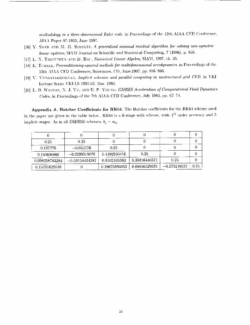
Appendix A. Butcher Coefficients for RK64. The Butcher coefficients for the RK64 scheme used

in the paper are given in the table below. RK64 is a 6 stage with scheme, with 4 th order a(:(:ura(:y and 5

implicit stages. As in all ESDIRK schemes, bj = a6j

0 0 0 0 0

0.25 0.25 0 0 0

0.137776 -0.055776 0.25 0 0

0.144636866 -0.2239319076 0.4492950416 0.25 0

0.098258783284 -0.59154424282 0.8102105383 0.28316440571 0.25

0.15791629516 0 0.18675894052 0.68056529531 -0.275240531

0

0

0

0

0

0.25

23

Form ApprovedREPORT DOCUMENTATION PAGE OMB No 0704-0188

Publicreportingburdenfor thiscollectionof informationisestimatedto average1 hourperresponse,includingthetimefor reviewinginstructions,searchingexistingdatasources.gatheringandmamtainlngthedataneeded,andcompletingandreviewingthecollectionof information.Sendcommentsregardingthisburdenestimateor anyotheraspectof thiscollectionofreformation,includingsuggestionsforreducingthis burden,to WashingtonHeadquartersServices,Directoratefor InformationOperationsandReports,1215JeffersonDavisHighway,Suite1204,Arlington.VA22202-4302,andto theOfficeof ManagementandBudget,PaperworkReductionProject(07040188),Washington,DC20503

1. AGENCY USE ONLY(Leaveblank) 2. REPORT DATE 3. REPORT TYPE AND DATES COVERED

November 2002 Contractor Report

4. TITLE AND SUBTITLE 5. FUNDING NUMBERS

HIGHER ORDER TIME INTEGRATION SCHEMES FOR THE

UNSTEADY NAVIER-STOKES EQUATIONS ON UNSTRUCTURED C NAS1-97046

MESHES WU 505-90-52-01

6. AUTHOR(S)

Giridhar Jothit]rasad, Dimitri J. Mavriplis, and David A. Caughey

7. PERFORMING ORGANIZATION NAME(S) AND ADDRESS(ES)

ICASE

Mail Stol) 132C

NASA Langley Research Center

Hampton, VA 23681-2199

g. SPONSORING/MONITORING AGENCY NAME(S) AND ADDRESS(ES)

National Aeronautics and Space Administration

Langley Research Center

Hampton, VA 23681-2199

8. PERFORMING ORGANIZATIONREPORT NUMBER

ICASE Report No. 2002-44

10. SPONSORING/MONITORINGAGENCY REPORT NUMBER

NASA/CR-2002-211967

1CASE Report No. 2002-44

11. SUPPLEMENTARY NOTES

Langley Techifical Monitor: Deimis M. Bushnell

Final ReportSubndtted to the Journal of Computational Physics.

12a. DISTRIBUTION/AVAILABILITY STATEMENT

Unclassified Unlimited

Subject Category 64Distribution: Nonstandard

Availability: NASA-CASI (301) 621-0390

12b. DISTRIBUTION CODE

13. ABSTRACT (Maximum 200 words)The efficiency gains obtained using higher-order lint)licit Runge-Kutta schemes as compared with the second-order

accurate backward difference schemes for the unsteady Navier-Stokes equations are investigated. Three different

algorithms for solving the nonlinear system of equations arising at each timestep are presented. The frst algorithm

(NMG) is a pseudo-time-stepping scheme which employs a non-linear full approximation storage (FAS) agglomeration

multigrid method to accelerate convergence. The other two algorithms are based on Inexact Newton's methods. The

linear system arising at each Newton step is solved using iterative/Krylov techniques and left preconditioning is usedto accelerate convergence of the linear solvers. One of the methods (LMG) uses Riehardson's iterative scheme for

solving the linear system at each Newton step while other (PGMRES) uses the Generalized Minimal Residual

method. Results demonstrating the relative superiority of these Newton's methods based schemes are presented.

Efficiency gains as high as 10 are obtained by combining the higher-order time integration schemes with the nloreefficient nonlinear soh'ers.

14. SUBJECT TERMSJacobian-free Newto11, Runge-Kutta methods, Navier-Stokes, multigrid, unstructured

grid

17. SECURITY CLASSIFICATIONOF REPORTUnclassified

_SN 7540-01-280-5500

18. SECURITY CLASSIFICATION 19. SECURITY CLASSIFICATIONOF THIS PAGE OF ABSTRACTUnclassified

15. NUMBER OF PAGES

28

16. PRICE CODE

A03

20. LIMITATIONOF ABSTRACT

!

Standard Form 298(Rev. 2-8g)Prescribed by ANSI Std. Z39 18

298-102