ENO and WENO schemes. Further topics and time Integration · PDF fileENO and WENO schemes....
28
ENO and WENO schemes. Further topics and time Integration Tefa Kaisara CASA Seminar 29 November, 2006
Transcript of ENO and WENO schemes. Further topics and time Integration · PDF fileENO and WENO schemes....

ENO and WENO schemes. Further topicsand time Integration
Tefa Kaisara
CASA Seminar
29 November, 2006
Short review Further topics Time Integration
Outline
1 Short reviewENO/WENO
2 Further topicsSubcell resolutionOther building blocks
3 Time IntegrationTVD Runge-Kutta methodsTVD multistep methodsLax-Wendroff procedure
Short review Further topics Time Integration
Outline
1 Short reviewENO/WENO
2 Further topicsSubcell resolutionOther building blocks
3 Time IntegrationTVD Runge-Kutta methodsTVD multistep methodsLax-Wendroff procedure
Short review Further topics Time Integration
ENO/WENO
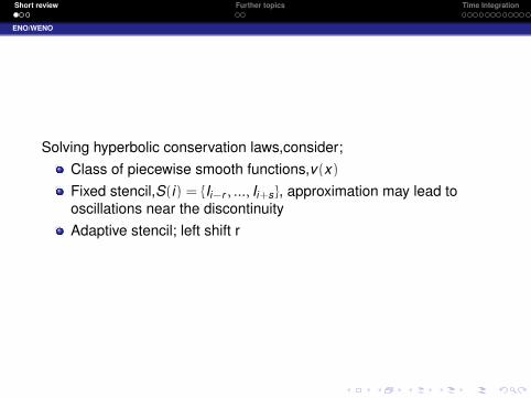
Solving hyperbolic conservation laws,consider;Class of piecewise smooth functions,v(x)
Fixed stencil,S(i) = {Ii−r , ..., Ii+s}, approximation may lead tooscillations near the discontinuityAdaptive stencil; left shift r
Short review Further topics Time Integration
ENO/WENO
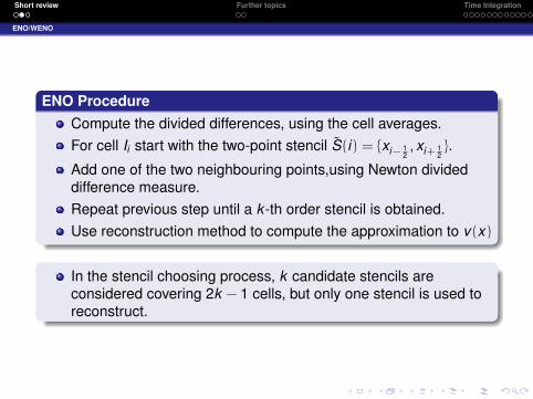
ENO ProcedureCompute the divided differences, using the cell averages.For cell Ii start with the two-point stencil S(i) = {xi− 1
2, xi+ 1
2}.
Add one of the two neighbouring points,using Newton divideddifference measure.Repeat previous step until a k -th order stencil is obtained.Use reconstruction method to compute the approximation to v(x)
In the stencil choosing process, k candidate stencils areconsidered covering 2k − 1 cells, but only one stencil is used toreconstruct.

Short review Further topics Time Integration
ENO/WENO
To improve the accuracy:
Assume a uniform grid, i.e. ∆xi = ∆x , i = 1, . . . , N. Consider the kcandidate stencils
Sr (i) = {xi−r , . . . , xi−r+k−1} r = 0, . . . , k − 1.
The reconstruction produces k different approximations to the valuev(xi+ 1
2) :
v (r)i+ 1
2=
k−1∑j=0
crj vi−r+j r = 0, . . . , k − 1 (1.1)
I WENO takes a convex combination of the v (r)i+ 1
2’s.

Short review Further topics Time Integration
Outline
1 Short reviewENO/WENO
2 Further topicsSubcell resolutionOther building blocks
3 Time IntegrationTVD Runge-Kutta methodsTVD multistep methodsLax-Wendroff procedure
Short review Further topics Time Integration
Subcell resolution
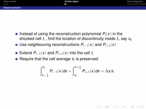
Instead of using the reconstruction polynomial Pi(x) in theshocked cell Ii , find the location of discontinuity inside Ii , say xs
Use neighbouring reconstructions Pi−1(x) and Pi+1(x)
Extend Pi−1(x) and Pi+1(x) into the cell IiRequire that the cell average vi is preserved:∫ xs
xi −12
Pi−1(x)dx +
∫ xi +12
xs
Pi+1(x)dx = ∆xi vi
Short review Further topics Time Integration
Other building blocks
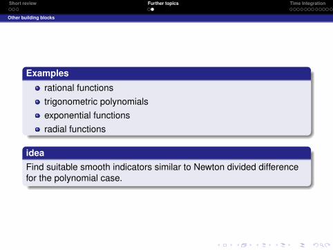
Examples
rational functionstrigonometric polynomialsexponential functionsradial functions
ideaFind suitable smooth indicators similar to Newton divided differencefor the polynomial case.

Short review Further topics Time Integration
Outline
1 Short reviewENO/WENO
2 Further topicsSubcell resolutionOther building blocks
3 Time IntegrationTVD Runge-Kutta methodsTVD multistep methodsLax-Wendroff procedure
Short review Further topics Time Integration
TVD Runge-Kutta methods
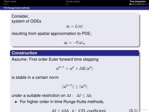
Consider,system of ODEs
ut = L(u)
resulting from spatial approximation to PDE;
ut = −f (u)x
ConstructionAssume: First order Euler forward time stepping
un+1 = un + ∆tL(un)
is stable in a certain norm
||un+1|| ≤ ||un||
under a suitable restriction on ∆t : ∆t ≤ ∆t1I For higher order in time Runge-Kutta methods,
∆t ≤ c∆t1 c : CFL coefficient (3.1)

Short review Further topics Time Integration
TVD Runge-Kutta methods
General Runge-Kutta method
u(i) =
i−1∑k=0
(αik uk + ∆tβik L(u(k))
), i = 1, . . . , m (3.2)
u(0) = un, u(m) = un+1
For αik ≥ 0, βik ≥ 0 ⇒ convex combination of Euler forward operators
∆t replaced byαik
βik∆t
Consistency;i−1∑k=0
αik = 1.

Short review Further topics Time Integration
TVD Runge-Kutta methods
LemmaThe Runge-Kutta method (3.2) is TVD under the CFL coefficient (3.1)
c = mini,k
αik
βik
provided; αik ≥ 0 and βik ≥ 0.
Short review Further topics Time Integration
TVD Runge-Kutta methods
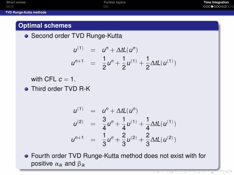
Optimal schemes
Second order TVD Runge-Kutta
u(1) = un + ∆tL(un)
un+1 =12
un +12
u(1) +12
∆tL(u(1))
with CFL c = 1.
Third order TVD R-K
u(1) = un + ∆tL(un)
u(2) =34
un +14
u(1) +14
∆tL(u(1))
un+1 =13
un +23
u(2) +23
∆tL(u(2))
Fourth order TVD Runge-Kutta method does not exist with forpositive αik and βik

Short review Further topics Time Integration
TVD Runge-Kutta methods
Considerαik ≥ 0 and βik negative
introduce an adjoint operator Lit approximates the same spatial derivatives as LTVD for first order Euler, backward in time:
un+1 = un − ∆t Lun
Short review Further topics Time Integration
TVD Runge-Kutta methods
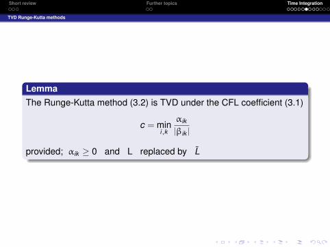
LemmaThe Runge-Kutta method (3.2) is TVD under the CFL coefficient (3.1)
c = mini,k
αik
|βik |
provided; αik ≥ 0 and L replaced by L

Short review Further topics Time Integration
TVD Runge-Kutta methods
Fourth order TVD R-K
u(1) = un +12
∆tL(un)
u(2) =649
1600u(0) −
1089042325193600
∆t L(un) +951
1600u(1) +
50007873
∆tLu(1)
u(3) =53989
2500000un −
1022615000000
∆t L(un) +4806213
20000000u(1) −
512120000
∆t L(u(1))
+2361932000
u(2) +7873
10000∆tL(u(2))
un+1 =15
un +110
∆tL(un) +6127
30000u(1) +
16
∆tL(u(1)) +7873
30000u(2)
+13
u(3) +16
∆tL(u(3))
Short review Further topics Time Integration
TVD Runge-Kutta methods
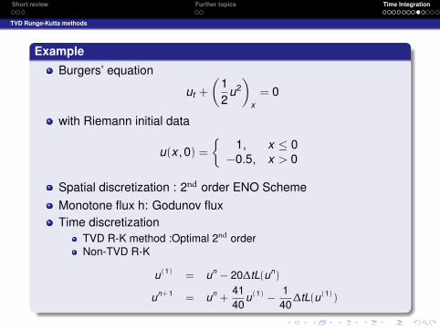
Example
Burgers’ equation
ut +
(12
u2)
x= 0
with Riemann initial data
u(x , 0) =
{1, x ≤ 0
−0.5, x > 0
Spatial discretization : 2nd order ENO SchemeMonotone flux h: Godunov fluxTime discretization
TVD R-K method :Optimal 2nd orderNon-TVD R-K
u(1) = un − 20∆tL(un)
un+1 = un +4140
u(1) −1
40∆tL(u(1))

Short review Further topics Time Integration
TVD Runge-Kutta methods
conclusionIt is much safer to use TVD Runge-Kutta Method for solvinghyperbolic problem.

Short review Further topics Time Integration
TVD multistep methods
ConstructionSimilar to Runge-kutta Methods
General From
un+1 =
m−1∑k=0
(αk un−k + ∆tβk L(un−k )) (3.3)
For αk ≥ 0, βk ≥ 0 ⇒ convex combination of Euler Forward operators
∆t replaced byβk
αk∆t
Consistency;m∑
k=0
αk = 1.

Short review Further topics Time Integration
TVD multistep methods
LemmaThe multi-step method (3.3) is TVD under the CFL coefficient (3.1)
c = mink
αk
βk
provided; αk ≥ 0 and βk ≥ 0
Short review Further topics Time Integration
TVD multistep methods
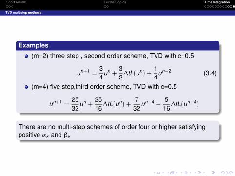
Examples
(m=2) three step , second order scheme, TVD with c=0.5
un+1 =34
un +32
∆tL(un) +14
un−2 (3.4)
(m=4) five step,third order scheme, TVD with c=0.5
un+1 =2532
un +2516
∆tL(un) +732
un−4 +516
∆tL(un−4)
There are no multi-step schemes of order four or higher satisfyingpositive αk and βk

Short review Further topics Time Integration
TVD multistep methods
LemmaThe multi-step method (3.3) is TVD under the CFL coefficient (3.1)
c = mink
αk
|βk |
provided; αk ≥ 0 and , L is replaced by L for βk negative.
one residue evaluation is needed per time stepstorage requirement is much bigger that Runge-Kutta methods
Short review Further topics Time Integration
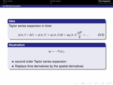
Lax-Wendroff procedure
IdeaTaylor series expansion in time:
u(x , t + ∆t) = u(x , t) + ut(x , t)∆t + utt(x , t)∆t2
2+ ... (3.5)
Illustration
ut = −f (u)x
second order Taylor series expansionReplace time derivatives by the spatial derivatives

Short review Further topics Time Integration
Lax-Wendroff procedure
ut(x , t) = −f (u(x , t))x = −f ′(u(x , t))ux(x , t)utt(x , t) = 2f ′(u(x , t))f ′′(u(x , t))(ux(x , t))2 + (f ′(u(x , t)))2uxx(x , t)
(3.6)
Substituting (3.6) into (3.5)Discretize the spatial derivatives of u(x , t) by ENO/WENOIntegrate the pde
ut(x , t) + fx(u(x , t)) = 0
over the region [xi− 12, xi+ 1
2]× [tn, tn+1] to obtain
un+1i = un
i −1
∆xi
(∫ tn+1
tnf (u(xi+ 1
2, t)) dt −
∫ tn+1
tnf (u(xi− 1
2, t)) dt
)(3.7)
Discretize time using suitable Gaussian quadrature
1∆t
∫ tn+1
tnf (u(xi+ 1
2, t)) dt ≈
∑α
ωαf (u(xi+ 12, tn + βα∆t))

Short review Further topics Time Integration
Lax-Wendroff procedure
replacing f (u(xi+ 12, tn + βα∆t)) by a monotone flux
f (u(xi+ 12, tn + βα∆t)) ≈ h(u(x±
i+ 12, tn + βα∆t)
use the Lax-Wendroff procedure to convert
u(x±i+ 1
2, tn + βα∆t) (3.8)
to u(x±i+ 1
2, tn) and its spacial derivatives at tn.

Short review Further topics Time Integration
Lax-Wendroff procedure
limitationsAlgebra is very complicated for multi dimensional systemsdifficult to prove stability properties for higher order methods
Short review Further topics Time Integration


![WLS-ENO: Weighted-Least-Squares Based Essentially Non ...jiao/papers/wls-eno-fvm.pdf · ENO scheme [24] and its closely related WENO schemes [2]. In a nutshell, the ENO is a WENO](https://static.fdocuments.in/doc/165x107/6117dbe78dfbd9699074d533/wls-eno-weighted-least-squares-based-essentially-non-jiaopaperswls-eno-fvmpdf.jpg)


![HERMITE WENO SCHEMES WITH STRONG STABILITY PRESERVING ...ccam.xmu.edu.cn/.../HWENO_multi_step_JCM_2014.pdf · results in [6] include the optimal explicit SSP linear Runge-Kutta methods,](https://static.fdocuments.in/doc/165x107/5f0d2ee57e708231d43914a8/hermite-weno-schemes-with-strong-stability-preserving-ccamxmueducnhwenomultistepjcm2014pdf.jpg)
![High Order Positivity- and Bound-Preserving Hybrid Compact-WENO Finite Difference ... order... · 2020. 4. 14. · and hybrid compact-ENO schemes [1] as well, at a lower computational](https://static.fdocuments.in/doc/165x107/60fe3dae4ee51b2a2263592f/high-order-positivity-and-bound-preserving-hybrid-compact-weno-finite-difference.jpg)