Seediscussions,stats,andauthorprofilesforthispublicationat:https://www.researchgate.net/publication/316789928

HigherOrderDynamicModeDecomposition

ArticleinSIAMJournalonAppliedDynamicalSystems·January2017

DOI:10.1137/15M1054924

CITATIONS

2

READS

141

2authors:

Someoftheauthorsofthispublicationarealsoworkingontheserelatedprojects:

HigherorderdynamicmodedecompositionViewproject

SoledadLeClaincheMartínez

UniversidadPolitécnicadeMadrid

18PUBLICATIONS82CITATIONS

SEEPROFILE

JoséM.Vega

UniversidadPolitécnicadeMadrid

159PUBLICATIONS1,519CITATIONS

SEEPROFILE

AllcontentfollowingthispagewasuploadedbySoledadLeClaincheMartínezon09May2017.

Theuserhasrequestedenhancementofthedownloadedfile.

SIAM J. APPLIED DYNAMICAL SYSTEMS c© 2017 SIAM. Published by SIAM under the termsVol. 0, No. 0, pp. 000–000 of the Creative Commons 4.0 license

Higher Order Dynamic Mode Decomposition∗

Soledad Le Clainche† and Jose M. Vega†

Abstract. This paper deals with an extension of dynamic mode decomposition (DMD), which is appropriate totreat general periodic and quasi-periodic dynamics, and transients decaying to periodic and quasi-periodic attractors, including cases (not accessible to standard DMD) that show limited spatialcomplexity but a very large number of involved frequencies. The extension, labeled as higher orderdynamic mode decomposition, uses time-lagged snapshots and can be seen as superimposed DMDin a sliding window. The new method is illustrated and clarified using some toy model dynamics,the Stuart–Landau equation, and the Lorenz system. In addition, the new method is applied to(and its robustness is tested in) some permanent and transient dynamics resulting from the complexGinzburg–Landau equation (a paradigm of pattern forming systems), for which standard DMD isseen to only uncover trivial dynamics, and the thermal convection in a rotating spherical shell subjectto a radial gravity field.

Key words. dynamic mode decomposition, Koopman operator, delayed snapshots, nonlinear dynamical sys-tems, transient dynamics, quasi-periodic attractors, complex Ginzburg–Landau equation, thermalconvection in spherical shells

AMS subject classifications. 35B10, 35B40, 35B41, 35C99, 37L15, 37L30, 37M99

DOI. 10.1137/15M1054924

1. Introduction. Dynamic mode decomposition (DMD) is closely related to (and inspiredby) Koopman-operator analysis [36, 43], initiated by Koopman [31] in 1931. DMD itself wasdeveloped by Schmid [48], and has become a useful tool for postprocessing massive spatio-temporal data in numerical and experimental fluid mechanics [49, 50, 51, 52, 32] and otherfields [28, 40]. The ability of DMD to extract relevant patterns makes this method potenti-ally useful in identifying nonlinear dynamics in many physical systems, but this applicationrequires some care since the standard DMD may give completely spurious results. The maingoal of this paper is to analyze the application of DMD to general (both low-dimensionaland infinite-dimensional) dynamical systems, which will require a nontrivial extension of themethod.

In order to fix ideas, DMD applies to spatio-temporal data organized in K equispacedJ-dimensional snapshots as

(1.1) vk ≡ v(tk) ∈ RJ for tk = t1 + (k − 1)∆t with k = 1, . . . ,K.

Thus, the spatial and temporal dimensions of the given data are J and K, respectively. Stan-

∗Received by the editors January 4, 2016; accepted for publication (in revised form) by T. Sauer December 20,2016; published electronically DATE.

http://www.siam.org/journals/siads/x-x/M105492.htmlFunding: This research was partially supported by the Spanish Ministry of Economy and Competitiveness, under

grant TRA2013-45808-R.†E.T.S.I. Aeronautica y del Espacio, Universidad Politecnica de Madrid, 28040 Madrid, Spain (soledad.leclainche@

upm.es, josemanuel.vega@upm.es).

1

2 SOLEDAD LE CLAINCHE AND JOSE M. VEGA

dard DMD relies on the following Koopman assumption:

(1.2) vk+1 = Rvk for k = 1, . . . ,K − 1

for a certain J × J-matrix R, which can be called the Koopman matrix (or operator). Forsimplicity in the exposition, this equation is assumed at the moment to be satisfied exactly,though it will only hold approximately in most applications (see below). The assumption(1.2) implies that the snapshots lie in the invariant subspace under the action of the Koopmangroup [58, 11], generated by R. This assumption leads to the following DMD representationof the snapshots:

(1.3) v(tk) =

M∑m=1

amum e(δm+iωm)(k−1)∆t for k = 1, . . . ,K,

where the exponents appear in complex conjugate pairs when the snapshots are real. This isa Fourier-like expansion that involves, not only the frequencies ωm, but also the growth ratesδm.

The linear time invariant (LTI) [60] system (1.2) is not assumed to be the actual physicalmodel that has produced the snapshots. In other words, the role of the linear system (1.2)is only instrumental in this context, as a means to compute the modes um, amplitudes am,growth rates δm, and frequencies ωm appearing in the Fourier-like expansion (1.3). Instead,the underlying physical model may well be nonlinear, and the snapshots (1.1) satisfying (1.2)may be particular outcomes of the system for a periodic (if δm = 0 and the frequencies ωm arecommensurable) or quasi-periodic (if δm = 0 and the frequencies ωm are incommensurable)attractor of the system, or for a transient approaching a periodic or quasi-periodic attractor(if δm ≤ 0).

Since any terms in (1.3) with the same exponents may be collected into a single term bysumming their coefficients, we assume (without loss of generality) that the various exponentsin (1.3) are distinct. In this case, the number of involved modes, M , can be called the spectralcomplexity, while the dimension of the subspace generated by the M DMD-modes, namely

(1.4) N = dim (span{u1, . . . ,uM}) ≤ min{M,J},

is the spatial complexity. The spatial complexity can be elucidated via either truncated properorthogonal decomposition (POD) [16] or truncated singular value decomposition (SVD) [25],which allows reducing the dimension of the snapshots set and, combined with the pseudo-inverse, also permits computing the Koopman matrix R. Once R has been calculated, thegrowth rates and frequencies appearing in (1.2) are related to the nonzero eigenvalues of R,µm, as

δm + iωm =1

∆tlogµm,

while the modes um are the associated eigenvectors; the amplitudes am can be computed byvarious means (see below). At the moment, it is convenient to note that, if (1.2) and (1.3) areconsistent with each other, then

HIGHER ORDER DYNAMIC MODE DECOMPOSITION 3

• The DMD modes appearing in (1.3) are linearly independent, as eigenvectors of amatrix associated with different eigenvalues.• The number of terms appearing in (1.3), namely the spectral complexity M , cannot

be larger than the spatial complexity N , which, invoking (1.4), means that M = N .In fact, ifM = N and conditions (1.2) and (1.3) are exact, then these conditions are equivalent.This is a fundamental limitation of standard DMD [48]. More general expansions (1.3), withM > N , cannot be obtained via standard DMD, which gives spurious results, even in thesimplest case in which the snapshots are identically of the form (1.3) (see the examples insection 3.1). Instead, according to Theorem D in Appendix A, the expansion (1.3) is consistent(always, for general M and N) with the following higher order Koopman assumption:

(1.5) vk+d = R1 vk + R2 vk+1 + . . .+ Rd vk+d−1 for k = 1, . . . ,K − d,

where d ≥ 1 is tunable. Summarizing, although the assumption (1.2) leads to the DMDexpansion (1.3), the converse is not true, namely not all expansions of the form (1.3) canbe calculated from the assumption (1.2). The more general assumption (1.5), instead, isequivalent to (1.3).

It must be noted that the spectral complexity M is larger than the spatial complexityN in dynamical systems of scientific and industrial interest. For instance, N = 3 in theLorenz system (considered in section 3.2), which exhibits chaotic dynamics (infinite spectralcomplexity) and also periodic attractors with very large spectral complexity M . On the otherhand, M may be larger than N in dissipative, infinite-dimensional systems modeled by partialdifferential equations. For example,

• The weakly nonlinear theory near a Hopf bifurcation in these systems is describedby a Stuart–Landau equation [26]. As further explained in section 3.3, the weaklynonlinear theory predicts transient dynamics involving a large number M of decayingmodes that are approximately contained in the two-dimensional center manifold builtaround the steady state, meaning that N = 3 < M .• Similarly, weakly nonlinear descriptions of quasi-periodic phenomena in these systems

(see [2] and references therein) may involve few spatial modes.• Fully nonlinear dynamics can behave similarly in these systems since, for large t,

the solution of many infinite-dimensional systems converges to a nonlinear, finite-dimensional inertial manifold [22], contained in a generally larger (but finite-dimensional,according to the Whitney embedding theorem [27]) N -dimensional linear manifold.The dynamics in this manifold may well be chaotic (e.g., transitional flows) and alsoexhibit attractors with large M (> N). A very clear example with finite-dimensionalinertial manifold where fairly complex dynamics occur is the complex Ginzburg–Landau equation, which will be considered in section 4. This is a very convenientpattern forming system to illustrate the methods in this paper because (i) it exhibitsfairly complex dynamics, (ii) it is a “normal form” that applies to a variety of oscilla-tory bifurcations in infinite-dimensional systems [19, 26], and (iii) it is simple enoughas to allow for fast numerical simulation. Also, this application suggests that higherorder dynamic mode decomposition (HODMD) may be very useful to analyze perio-dic and quasi-periodic phenomena in pattern forming systems. Let us note here that

4 SOLEDAD LE CLAINCHE AND JOSE M. VEGA

identifying and computing quasi-periodic attractors in infinite-dimensional systems isa subtle matter [45, 46].

The counterpart of standard DMD using the assumption (1.5) will be labeled as HODMD,and will be seen in this paper to be a fairly precise and robust means to compute the expansion(1.3) for sets of snapshots resulting from general periodic and quasi-periodic dynamics, namelyconsistent with (1.3), with arbitrary finite values of the spectral and spatial complexities. Inany event, irrespective of whether the correct DMD expansion is calculated using standardDMD (which can be seen as a particular case of HODMD) or HODMD, the continuous ex-tension of (1.3),

(1.6) v(t) =

M∑m=1

um e(δm+iωm)(t−t1) for t1 ≤ t ≤ tK ,

may be used to reconstruct (very general, transient, or permanent) nonlinear dynamics. Forpermanent dynamics (when all δm = 0), (1.6) can be seen as interpolation in the time variable,while for transient dynamics (with δm ≤ 0), skipping in (1.6) those terms with δm < 0 permitsanticipating the final attractor for t� 1 from transient behavior, which involves extrapolationand, as noticed elsewhere [3], may be used to reduce the CPU time required to approachthe final attractors using numerical simulation; this CPU time may be huge near bifurcationpoints.

The good performance of HODMD can be attributed to the fact that, according to Theo-rem D in Appendix A, the assumption (1.5) is general enough as to allow for general spatio-temporal behaviors of the form (1.3). Another explanation of the improved performance ofHODMD follows by interpreting (1.5) as a modified form of (1.2) containing also time-laggedsnapshots. Namely, (1.5) can also be written as

(1.7) vk+1 = R vk,

where the modified snapshots vk and the modified Koopman matrix R are defined as

vk ≡

vkvk+1

. . .vk+d−2

vk+d−1

, R ≡

0 I 0 . . . 0 00 0 I . . . 0 0. . . . . . . . . . . . . . . . . .0 0 0 . . . I 0R1 R2 R3 . . . Rd−1 Rd

,(1.8)

with I = the J × J unit matrix. In fact, the algorithm presented in this paper to performHODMD, which will be called the DMD-d algorithm, roughly consists of applying standardDMD to the enlarged snapshots defined in (1.8). The good performance of the computationsbased on (1.7) could be seen as consistent with the use of sliding windows in the improvementof the fast Fourier transform (FFT) known as power spectral density (PSD) [38]. A morerelevant explanation follows noting that if the spatial complexity of the original snapshots issmaller than the spectral complexity, including the time-lagged snapshots in (1.8) recoversthe missing degrees of freedom and increases the spatial complexity in the enlarged snapshotsas to make it equal to the spectral complexity. This is consistent with the method of delay-coordinate embedding for state space reconstruction of an attractor using time-series of a

HIGHER ORDER DYNAMIC MODE DECOMPOSITION 5

limited number of observables (even scalar observables). In this method, the number ofobservables is increased by using time-lagged observables (see also [58, 59] for alternativeways of extending the space of observables); delayed information has also been recently usedin model identification [12]. The method of delay-coordinate embedding relies on seminalideas by Packard et al. [37], which were formalized by Takens [54] in his delay-embeddingtheorem (see also [44] for extensions of this theorem), and further pursued by Broomheadand King [10]. In this sense, HODMD can be seen as a synergic combination of standardDMD and Takens’ delay embedding and could be useful for the delay-embedding community,which is very interested in forecasting. However, most of the current forecasting methodsare restricted to stationary time-series, which are analyzed using classical techniques such asthe method of analogs [34] and local linear forecasting [21, 13]. These methods have beenrecently revisited, combined with diffusion maps [62, 9] and the Koopman operator [24], andgeneralized to a probabilistic framework for stochastic systems [42, 7, 8]. In contrast to theselocal linear methods, HODMD is a global linear method that provides all involved frequenciesand growth rates simultaneously. Moreover, by its own nature, the outcomes of HODMD mayinvolve nonzero decaying rates in (1.6), which permits extrapolation (and thus dealing withnonstationary time series) while the delay-embedding methods mentioned above are all basedon interpolation on stationary time series.

Although, for simplicity in the presentation, (1.2), (1.3), and (1.5) were assumed above tobe exact, these equations are usually only approximate in typical applications, due to eitherthe presence of noise or the fact that only a limited accuracy is sought. In the latter case, thespatial complexity M and the spectral complexity N depend on the required accuracy. In fact,the accuracy may be an issue [61, 29] when calculating the DMD expansion (1.3). Concerningnoise, this is filtered out by the preliminary application of SVD (whose ability to filter outnoise is well known [53]), which is performed as the previous step to dimension-reducingthe snapshots set and reinforced through the use of delayed snapshots (whose insensitivityto noise is well documented [6]). In this context, it is necessary to robustly capture thespatio-temporal redundancies, which requires having enough data in both space and time.Concerning the selected snapshots, the sampling frequency must be somewhat large comparedto the largest frequency appearing in (1.3) and the sampled timespan be somewhat largecompared to 2π/ωmin, where ωmin is the smallest frequency in (1.3). These conditions imply,in particular, that K should be such that

(1.9) K �M.

The good performance of the standard DMD and HODMD methods requires testing theaccuracy of the reconstructed snapshots via the approximation (1.3) obtained by these met-hods. However, the aim is not using DMD-like methods as a data-processing tool, just toobtain good data-reconstructions, but to uncover the underlying dynamics. The differencebetween both goals will be made clear in this paper (see section 3.1) noting that high-order(namely, exhibiting very small amplitudes am) DMD modes in (1.3) may be useful to obtaingood data reconstructions, but still be associated with “errors” resulting from the finite sam-pled timespan, the finite sampling frequencies, and/or noise. In other words, these smallamplitude modes could be dynamically spurious. Thus, accuracy is not enough, but robust-

6 SOLEDAD LE CLAINCHE AND JOSE M. VEGA

ness (against changes in the sampling frequency, the sampled time interval, and the index d)is also necessary to identify the dynamically relevant DMD modes.

On the other hand, HODMD may be used to recover the relevant frequencies in periodicand quasi-periodic dynamics using a very limited amount of noisy data. This is because, asalready mentioned, HODMD takes advantage, not only of the spatial redundancies (via thetruncated SVD step that is performed at the outset), but also of the temporal redundancies(through the time-lagged snapshots). This is of interest to, e.g., minimizing the number ofsensors in experimental tests (e.g., of accelerometers in aeroelastic wind tunnel and flighttests [30]). In fact, standard DMD is somewhat similar to the so-called autoregressive movingaverage (ARMA) method [35], which is already used in aeroelasticity. It would be interestingto know how the time-lagged snapshots considered in the HODMD method improves ARMA,though this application is well beyond the scope of this paper.

The examples and applications below are performed using MATLAB. Sufficient details aregiven in all cases, allowing the reader to reconstruct and check results.

The remainder of this paper is organized as follows. The HODMD method is introduced insection 2, and the new method is developed in the context of the standard DMD method. Thenew ideas and the performance of the method are illustrated in section 3, where several exam-ples are considered that include both simple toy models (in section 3.1 and low-dimensionalsystems (in sections 3.2 and 3.3). In particular, for the Lorenz system considered in section3.2, HODMD will be used to recover the final attractors from transient dynamics. The morecomplex periodic and quasi-periodic attractors appearing in the complex Ginzburg–Landauequation (CGLE) will be considered in section 4, where the ability of HODMD to recover therelevant frequencies in complex dynamics using a limited amount of noisy data will also betested and compared with FFT and PSD. The HODMD method will be applied in section 5to the three-dimensional thermal convection in a rotating spherical shell subject to a radialgravity field, a problem that is of fundamental interest in geophysical and astrophysical fluiddynamics [17]. This paper ends with some concluding remarks in section 6.

2. Higher order dynamic mode decomposition. For convenience, the standard DMDmethod is first revisited and reformulated in the spirit of this paper. Then the standard DMDis extended using delayed snapshots, which gives the HODMD method. Below, we consider se-veral snapshot matrices (whose columns are snapshots), denoted as V k2

k1= [vk1 ,vk1+1, . . . ,vk2 ].

For instance, the full snapshot matrix is

V K1 = [v1, . . . ,vk].

The aim is to calculate the DMD expansion

vk ' vDMDk ≡

M∑m=1

amume(δm+iωm)(k−1)∆t for k = 1, . . . ,K,(2.1)

in a robust and precise way.

2.1. Standard DMD revisited and reformulated: The DMD-1 algorithm. StandardDMD relies on the assumption (1.2), namely

(2.2) vk+1 ' Rvk for k = 1, . . . ,K − 1,

HIGHER ORDER DYNAMIC MODE DECOMPOSITION 7

which can be written in matrix form (in terms of snapshot matrices) as

(2.3) V K2 ' RV K−1

1 .

These approximate equations, and many other appearing below, could be written as exactequations with a residual. For instance, (2.4) could be written as V K

1 = U ΣT> + R, wherethe residual depends on the neglected singular values, σ2

N+1 + · · · , and associated modes, and

is readily seen to exhibit a Frobenius norm ‖R‖Fro =√σ2N+1 + · · ·. Likewise, the norm of

the residual in the remaining approximate equations could be estimated noting that theseequations are obtained upon direct application of truncated SVD (for which well known errorestimates are available [25]) or the pseudoinverse (which also relies on SVD). Moreover, theseestimates could be used to obtain an a priori error estimate for the snapshots reconstructionvia the DMD expansion (2.1). However, none of these will be done below to avoid both a tooinvolved analysis and fairly messy equations, which would divert from the main focus of thepaper. In any event, standard DMD and HODMD are both postprocessing methods, and theactual reconstruction error can well be calculated a posteriori.

The (somewhat straightforward and fairly similar to the method proposed by Schmid [48])method to calculate the standard DMD expansion is now described. The method proceeds inthree steps, considered in the following subsections.

2.1.1. Step 1: Dimension reduction. This step is performed by applying truncated SVD(implemented in the MATLAB command “svd”, option “econ”) to the full snapshot matrix,as

(2.4) V K1 ' U ΣT>, with U>U = T>T = the N ×N unit matrix,

where Σ is the diagonal matrix containing the retained SVD singular values sorted in decre-asing order, σ1, σ2, . . . , σN , and the (orthonormal) columns of the J × N matrix U and theK ×N matrix T are the spatial and temporal SVD-modes, respectively. Invoking well knownSVD formulae [25], the number N of retained modes is selected in terms of the rank of thesnapshots matrix, R ≤ min{J,K}, to be such that

(2.5) EE (N) ≡σ2N+1 + . . .+ σ2

R

σ21 + . . .+ σ2

R

≤ ε1,

where EE (N) is the relative root mean square (RMS) error of the approximation (2.4). Thethreshold ε1 is tunable and can be selected in view of the singular values distribution, usingthe error estimate (2.5). The default value could be ε1 = 10−8.

Now, (2.4) can also be written as

(2.6) V K1 ' U V

K1 ,

where the reduced snapshot matrix is defined as

(2.7) VK1 = ΣT>(≡ U>V K

1 ).

8 SOLEDAD LE CLAINCHE AND JOSE M. VEGA

The rows of the N × K-matrix VK1 are proportional to the SVD temporal modes and can

thus be seen as rescaled temporal modes. Rescaling is important to get consistent results

in the dimension-reduced formulation; see below. The columns of VK1 will be called the

reduced snapshots and exhibit a much smaller dimension than the original snapshot matrix ifN � J (the usual case when simulating infinite-dimensional systems). Thus, it is this reducedsnapshot matrix that will be used below in all computations. In particular, (2.6) implies thatthe snapshots and reduced snapshots are such that

(2.8) vk ' U vk.

Similarly, the counterpart of the DMD expansion (2.1) for the reduced snapshots is

vk ' vDMDk ≡

M∑m=1

amume(δm+iωm)(k−1)∆t for k = 1, . . . ,K,(2.9)

with

um = U um.

2.1.2. Step 2: Computation of the reduced Koopman matrix and the DMD modes.Premultiplying (2.2) and (2.3) by UT and invoking (2.8) yields

(2.10) vk+1 ' R vk or VK2 ' R V

K−11 with R = U>RU .

The N ×N -matrix R will be called the reduced Koopman matrix and is calculated using the

pseudoinverse, as follows. Standard (no truncation) SVD applied to the matrix VK−11 leads

to

(2.11) VK−11 = UΣ T

>,

where, assuming that N ≤ K−1 (see (1.9)), the N×N matrix U and the (K−1)×N matrix

T are such that U>U = UU

>= unit matrix, T

>T = unit matrix, and the N ×N diagonal

matrix Σ is nonsingular and (because of the rescaling (2.7)) is very close to its counterpartin (2.4), Σ. Substituting (2.11) into (2.10) and postmultiplying the resulting equation by

T Σ−1

U>

leads to

R = VK2 T Σ

−1U>.

Now, once the reduced snapshot matrix R has been calculated, its eigenvectors qm, rescaledas

(2.12) ‖qm‖/√J = 1,

and eigenvalues µm readily yield the modes, growth rates, and frequencies appearing in theDMD expansions (2.1) and (2.9) as

(2.13) um = qm, um = Uqm, δm + iωm =1

∆tlogµm.

HIGHER ORDER DYNAMIC MODE DECOMPOSITION 9

The rescaling (2.12) means that the RMS of the modes is 1, which makes the mode amplitudesam as independent as possible from J . The amplitudes am are left aside at the moment.

Now, this calculation is readily seen to differ from that in [48, p. 9] only in one point.The projection matrix U is calculated here in (2.4) by applying SVD to the whole snapshotmatrix V K

1 , while Schmid [48] calculates U by applying SVD to the smaller snapshot matrixV K−1

1 (ignoring the last snapshot). If the number of snapshots K � 1 (the usual case), thenboth calculations give very similar results. In fact, the method in [48, p. 9] gives almostidentical results as DMD-1 in all calculations performed in this paper and will not be furtherconsidered.

2.1.3. Step 3: Computation of the DMD mode amplitudes. The DMD amplitudes arenow calculated using the reduced DMD expansion (2.9), which, invoking (2.13), can also bewritten as

vk 'M∑m=1

amqmµk−1m for k = 1, . . . ,K.(2.14)

Since the dimension of the (known) reduced snapshots vk is N (= M in the present case) andthe eigenvectors qm are linearly independent, each of these equations uniquely determines theamplitudes am. The whole system of equations, instead, is highly overdetermined if K � 1(the usual case), but can be solved using the pseudoinverse, which represents a minimizationof the least-squares-error in the approximation (2.14) and is essentially equivalent to the so-called optimized DMD method [18]. This step is performed by rewriting (2.14) in matrix formas

(2.15) La = b,

where the (NK ×M)-matrix L, the unknown amplitudes vector a, and the forcing term bare defined as

(2.16) L =

Q

QM. . .

QMK−1

, a =

a1

a2

. . .aM

, b =

v1

v2

. . .vK

.Here, L is exactly the observability matrix for a linear system with observation given bythe M ×M -matrix Q = [q1, . . . , qM ] (formed by the eigenvectors) and dynamics given bythe M × M diagonal matrix M (formed by the associated eigenvalues, µ1, . . . , µM ). Thepseudoinverse is calculated by applying standard SVD (no truncation) to the matrix L as

(2.17) L = U1ΣU>2 ,

with the (NK ×M)-matrix U1 and the M ×M -matrix U2 such that

(2.18) U>1 U1 = U

>2 U2 = U2 U

>2 = the M ×M unit matrix.

10 SOLEDAD LE CLAINCHE AND JOSE M. VEGA

Substituting (2.17) into (2.15), premultiplying the resulting equation by U2Σ−1

U>1 , and

invoking (2.18) yields

(2.19) a = U2Σ−1

U>1 b.

As a final step, the mode amplitudes are all set ≥ 0 by changing sign in both am and qm whenneeded in the expansion (2.14). This completes the calculation of the amplitudes, which isusually the most computationally expensive step if K � 1 (the usual case).

Finally, the DMD modes can be reordered sorting the mode amplitudes in decreasingorder, and a smaller number of modes, M , may be selected imposing that

(2.20) aM+1/a1 < ε,

for some tunable (small) threshold ε.

2.1.4. Summary of the DMD-1 method. Summarizing, the following algorithm has beendeveloped to apply standard DMD to the snapshots (1.1). As a first step, truncated SVD isapplied to the snapshot matrix (see (2.4)), with the number of retained terms as defined in

(2.5), for some tunable threshold ε1. Then, the reduced snapshot matrix VK1 is calculated

using (2.6)–(2.7). The M eigenvectors qm and eigenvalues µm of R and the pseudoinversesolution of (2.16) (with the additional truncation of the DMD modes performed using (2.20))yield the ingredients of the DMD-expansion (2.1) using (2.13) and (2.19).

For convenience, this algorithm will be labeled as the DMD-1 algorithm. Since this algo-rithm relies on the assumption (2.10) (which is typically not known a priori), consistency ofthe results requires that

(2.21)∥∥∥V K

2 − RVK−11

∥∥∥2

/∥∥∥V K2

∥∥∥2� 1.

If this condition does not hold, then standard DMD gives a spurious approximation and themore general HODMD method, considered in the next subsection, should be used.

2.2. The higher order dynamic mode decomposition: DMD-d algorithm with d > 1.As anticipated in the introduction, HODMD relies on the higher order Koopman condition(1.5), namely

(2.22) vk+d ' R1 vk + R2 vk+1 + · · ·+ Rd vk+d−1 for k = 1, . . . ,K − d.

This more general condition is now treated in a similar way as we did with the assumption(2.2) in section 2.1, in three steps described in the following subsections.

2.2.1. Step 1: Dimension reduction. To begin with, we perform exactly the same dimen-sion reduction developed in step 1 of the DMD-1 method (see section 2.1.1), using (2.4)–(2.7)with a convenient threshold ε1, which yields exactly the same projection equation, namely(2.8). This is rewritten here for convenience as

(2.23) vk ' U vk.

HIGHER ORDER DYNAMIC MODE DECOMPOSITION 11

Using this, the counterpart of (2.22) in the reduced linear manifold is

(2.24) vk+d ' R1 vk + R2 vk+1 + · · ·+ Rd vk+d−1 for k = 1, . . . ,K − d.

As anticipated in the introduction, this equation can be seen as a modified Koopman equationand written as

vk+1 ' R vk,

where the modified snapshots vk and the modified Koopman matrix R are

vk ≡

vkvk+1

. . .vk+d−2

vk+d−1

, R ≡

0 I 0 . . . 0 00 0 I . . . 0 0. . . . . . . . . . . . . . . . . .0 0 0 . . . I 0

R1 R2 R3 . . . Rd−1 Rd

.(2.25)

Here, I and 0 are the N×N unit and zero matrices, respectively. Note that the modified snaps-hots vk are of dimension dN and the modified Koopman matrix R is a (dN × dN)-matrix,which may be fairly large but still reasonable. In fact, this matrix will not be calculatedbelow because the set of snapshots vk will be further dimension-reduced in the next step.Because d and K are usually fairly large, this step is usually fairly computationally expensive.Nonetheless, the spatial dimension reduction performed above (see (2.23)) has been essentialbecause if this were not performed, the dimension of the counterpart of the modified snapshotmatrix (see (2.26)) would be a (Jd × Jd) × (K − d + 1)-matrix. For typical applications inspatially three-dimensional fluid flows, J ∼ 107. Since K ∼ 1000 and d ∼ 100 for typicalquasi-periodic dynamics in infinite-dimensional systems (see below), the method would beabsolutely impractical without the spatial dimension reduction. In addition, the spatial di-mension reduction will not permanently remove information since Takens’ delay-embeddingtheorem guarantees that the full state can be reconstructed from any generic observable. So,introducing the lagged snapshots in the next section will reconstruct the variables necessaryto reconstruct the state.

2.2.2. Step 2: Computation of the DMD modes. The DMD-d method proceeds byapplying steps 1 and 2 in the DMD-1 method (see sections 2.1.1 and 2.1.2, respectively) tothe modified snapshot matrix (with vk as defined in (2.25))

(2.26) VK−d+11 = [v1, . . . , vK−d+1],

which is of order (dN)× (K− d+ 1). Note that when step 1 in the DMD-1 method is appliedto this snapshot matrix, then a dimension reduction results, which is an additional dimensionreduction to that performed in step 1 above and is made using the counterpart of (2.5), namely

(2.27) EE (N) ≡σ2N+1 + · · ·+ σ2

R

σ21 + · · ·+ σ2

R

≤ ε1 with R = min{dN, k − d+ 1}.

The threshold ε1 may coincide with its counterpart in the first dimension reduction performedin step 1 above (see section 2.2.1) or not. The outcome of DMD-1, step 2 (using (2.13)) is a set

12 SOLEDAD LE CLAINCHE AND JOSE M. VEGA

of DMD modes, qm, growth rates, δm, and frequencies ωm. Consistently with the definition(2.25) of the modified snapshots to whom DMD-1 has been applied, the N first componentsof qm (rescaled as indicated in (2.12)) give the reduced DMD-modes qm for the reduced DMDexpansion

vk ' vDMDk ≡

M∑m=1

amqme(δm+iωm)(k−1)∆t for k = 1, . . . ,K,(2.28)

which is the counterpart of (2.1). The growth rates and frequencies are precisely those com-puted in the application of the DMD method to the modified snapshot matrix (2.26).

2.2.3. Step 3: Computation of the DMD mode amplitudes. Once the reduced DMDmodes, qm, growth rates δm and frequencies ωm have been calculated, the DMD amplitudesam are calculated precisely as we did for the DMD-1 algorithm in section 2.1.1. Namely, theamplitudes in (2.28) are calculated by rewriting (2.28) in the form (2.14) and calculating theamplitudes vector via the pseudoinverse of the matrix L. A further truncation using (2.20) isalso performed. This completes the derivation of the reduced DMD expansion (2.28). As inthe DMD-1 method, this is usually the most computationally expensive step.

2.2.4. Summary of the DMD-d method, with d > 1. Summarizing the above, given aset of snapshots vk and an index d > 1, the snapshots are dimension reduced as explained instep 1 (see section 2.2.1), which gives the reduced snapshots vk defined in (2.23). The reducedmodes qm, growth rates δm, and frequencies ωm appearing in the reduced DMD expansion(2.28) are calculated as explained in section 2.2.2 and the mode amplitudes am, as explainedin section 2.2.3. Premultiplying the reduced expansion (2.28) by the projection matrix Uappearing in (2.23) yields the DMD expansion (2.1), with um = Uqm.

2.3. Practical implementation and calibration of the DMD-d algorithm. The DMD-1and DMD-d algorithms developed above are straightforwardly implemented in MATLAB. Infact, as developed, the methods (and all formulae) are applicable to both real and complexdata, as automatically performed in MATLAB by using the command ′ for the transpose >.As anticipated, these algorithms can be used, in principle, either (i) to reconstruct the set ofgiven snapshots (using the method as a data processing tool) or (ii) to uncover the underlyingdynamics, which is more subtle. The goal (ii) requires identifying the right damping rates andfrequencies and permits extrapolating the identified dynamics for large t.

Whatever the goal, these methods exhibit various tunable parameters, namely, the sampledtime interval, the number of snapshots K, the threshold ε1 used in SVD truncation (see(2.5)), the threshold ε defining the retained modes (see (2.20)), and the index d for theDMD-d method, which should be chosen in each particular application. Note that condition(2.21) is a very useful means to elucidate whether the standard method is appropriate or not.When DMD-1 is not appropriate, the calibration of the index d > 1 deserves some attention.Obviously, d must not be too close to 1. On the other hand, when applying the DMD-dmethod, the modified snapshots matrix (2.26) contains K − d modified snapshots (of sizedN), meaning that d > 1 must not be too close to K, to avoid that only a small number ofmodified snapshots are really used by the method. As a consequence, d must be chosen inan appropriate interval that, fortunately, is usually fairly wide, as it will be repeatedly seen

HIGHER ORDER DYNAMIC MODE DECOMPOSITION 13

below. The appropriate values of d obviously depend on the involved dynamics, the sampledtime interval, and the sampling frequency. For a given dynamics and sampled interval, d scaleswith the sampling frequency, namely with the number of snapshots K for a given sampledtimespan. In other words, if K is doubled, d should be doubled, too. This conclusion is furtherjustified in Appendix A.

If the method is to be used as a purely data processing tool, the reconstruction errorshould be made as small as possible. The accuracy of the reconstruction will be measuredbelow in terms of the relative RMS error, defined as

(2.29) RRMSE ≡

[∑Kk=1

∥∥vk − vDMDk

∥∥2

2∑Kk=1 ‖vk‖

22

]1/2

.

If, instead, the method is used to capture the relevant dynamics, then it must be ensuredthat the approximation captures well the dynamically relevant modes, which could, of course,be identified beforehand by other means (i.e., physical relevance). However, in the absence ofa priori information, the relevant modes can be identified elucidating the consistency of theresults when the parameters of the method are varied. In particular, consistency requires thatthe retained frequencies and growth rates be stable when the sampled time interval is shiftedor enlarged and the index d is varied. In other words, the DMD-d parameters can be tunedusing standard statistical cross-validation methods. This will be the means to distinguishbetween the relevant and spurious modes below. It must be kept in mind that spurious modesare to be expected due to the unavoidable errors, which in practice come from two sources:

• Numerical and experimental errors that are already present in the snapshots. If theRMS level of these errors is known beforehand, then they can be filtered out by anappropriate selection of the threshold ε1 appearing in (2.5), taking advantage of thewell known [57] error-filtering ability of POD/SVD. If, instead, the error level is notknown, but the errors are uncorrelated with the physically meaningful data, then theywill promote a change of tendency in the usual semilogarithmic plot of the singularvalues of the primary SVD performed in (2.5) versus the retained number of modes.This change of tendency can help to identify the error level; see Figure 1.• Errors that are promoted by the method itself, such as round-off or truncation errors,

finite-sampled-timespan errors, finite-sampling-frequency errors, and errors resultingfrom the various pseudoinverse calculations above. Because of these errors, the ap-propriate number of retained DMD modes in the DMD expansions will not generallycoincide with its maximum possible number. It is precisely because of this that thelast truncation (2.20) was performed. The threshold ε in this truncation should beselected attending to the robustness of the results when the various parameters of themethod are varied, as explained above.

Once the dynamically relevant modes have been identified, they naturally provide thestructure of the attractor in permanent dynamics. Also, in transient dynamics, the relevantDMD-expansion (1.3) can be used to extrapolate to t � 1, which gives an approximation ofthe final attractor. The extrapolation is performed by just ignoring in (1.3) those DMD modeswith negative δm, which generally gives a smaller number of asymptotic modes, M∞. It mustbe noted that, because of errors, some relevant asymptotic modes may exhibit a small-but-

14 SOLEDAD LE CLAINCHE AND JOSE M. VEGA

nonzero |δm|. Thus, a threshold ε2 � 1 is defined and the growth rate of those modes with|δm| < ε2 is set to zero before performing extrapolation. When comparing two extrapolations,a relative time-shift t0 may be present, which must be dealt with as explained in the nextparagraph.

Consistency between DMD-d reconstructions of attractors using different snapshots setsis problematic because of the possible time-shifts that naturally appear. In other words, twoDMD reconstructions can only be required to be close to each other up to a time shift. Forperiodic dynamics, the shift must be smaller than the period and it can be calculated upon(nonlinear) least squares fit. For quasi-periodic attractors, instead, the time shift can beextremely large and the least square fit be impractical. Thus, in these more involved cases,the comparison will be made below only in terms of the DMD amplitudes and frequencies.

3. Illustration of the HODMD method. Let us now illustrate the HODMD method inboth several toy model dynamics and two low-dimensional systems: the Lorenz system andthe Stuart–Landau equation.

3.1. Some toy model dynamics. A simple but quite illustrative application of the met-hods proceeds as follows: Select randomly N orthonormal complex vectors of dimensionJ > N , w1, . . . ,wN , and construct M > N linear combinations,

(3.1) um =N∑j=1

αjwj ,

with randomly selected coefficients αj , such that the Euclidean norm of the vectors um is√J

(see (2.12)). Here, we are assimilating the various components of u as “spatial coordinates.”With these, construct the following toy-model dynamics:

u(t) =

M∑m=1

amumeiωmt,

with the amplitudes am and the frequencies ωm selected below. Because of the randomcharacter of this example (which has been included to avoid any bias in the example), theperformance of the methods will slightly vary from one run to another, but the results willbe essentially consistent. Now, K > M equispaced snapshots are selected in the interval0 ≤ t ≤ 1. Note that these J ×K data are a “simple” instance of the DMD expansion (2.1)that, by construction, exhibits spatial and spectral complexities exactly equal to N and M ,respectively. Once the various random selections above have been fixed, several interestingcases to illustrate the methods will be considered by appropriately varying the integers J , K,M , and N .

To begin with, we set J = 100, K = 1000, M = N = 10 (i.e., equal spectral and spatialcomplexities), and select the amplitudes and frequencies as

(3.2) am = 10−m/2, ωm = 10m for m = 1, . . . ,M.

Note that the sampling frequency is K = 1000, namely ten times larger than the largestfrequency, ω1 = 100. Since M = N , the spectral and spatial complexities coincide and the

HIGHER ORDER DYNAMIC MODE DECOMPOSITION 15

standard DMD-1 algorithm should do a good job. In fact, setting

(3.3) ε1 = 10−6, ε = 10−6,

the DMD-1 algorithm calculates the frequencies with a relative error 10−13 and reconstructsthe snapshots with relative RMS error, as defined in (2.29), RRMSE ∼ 10−12. The algorithmDMD-d provides slightly better results for d in the range 1 < d < 400.

Now, we maintain the parameters of the method, (3.3), the spectral complexity M = 10,and the amplitudes and frequencies defined in (3.2), but decrease the spatial complexity toN = 5. Since N = 5 < M = 10, the algorithm DMD-1 is only able to recognize five modes,with frequencies

ω1 = 55.85, ω2 = 48.28, ω3 = 27.40, ω4 = 93.03, ω5 = 66.69,

which compared with (3.2) are seen to be spurious; the reconstruction relative error RRMSEis ∼ 10−2. Applying the HODMD algorithm DMD-d, with d = 50 (which is somewhat optimalfor this case), instead, recovers both the M = 10 frequencies defined in (3.2) with a relativeerror ∼ 10−13 and the snapshots within a relative error RRMSE∼ 10−13. Slightly increasingand decreasing d (to, e.g., 80 and 20, respectively) the very small reconstruction errors areessentially maintained.

Let us now add some noise to the data. Specifically, we add uniformly distributed positivenoise (using the MATLAB command rand) with size εnoise = 5 · 10−7. Note that the noise ispositive and thus exhibits a nonzero mean. Repeating the two cases considered above to thisnoisy data, with ε1 = ε = 10−6 (both two times larger than the noise), the following resultsare obtained:

a. For the case M = N = 10, the relative RMS reconstruction (comparing with the cleansolution) is RRMSE ∼ 10−4 and ∼ 10−7 using the algorithms DMD-1 and DMD-300(note that now the convenient value of d is larger than in the clean case), respectively.Thus, both the standard DMD and HODMD are able to filter errors out (despite thefact that the errors are positive), though HODMD gives much better results.

b. For the case M = 10, N = 5, DMD-1 fails, as above, since it only recognizes five modesand reconstructs the solution with RRMSE ∼ 10−2. DMD-300 (note that d is largernow than for clean data), instead, recovers the ten frequencies with a relative error∼ 10−9 and reconstructs the solution with RRMSE ∼ 10−7 (which is fairly smallerthan the added noise!). Again, HODMD is quite robust in connection with varyingthe index d, and the results improve if the sampled interval and/or the number ofsnapshots is increased.

As expected, the noise reduces the performance of both methods, but the new HODMDmethod gives far more robust estimates and reconstructions. This is because, as anticipated,HODMD takes full advantage of both the spatial and temporal redundancies in the given data.Note that the threshold ε = 10−6 has been chosen as somewhat larger than the error level,5 · 10−7. If the latter were not known in advance, then it could be guessed from the singularvalue distribution in the SVD that is performed in the method. For instance, in the two cases(a and b) considered above, using DMD-1 and DMD-300, the singular value distributions areplotted in Figure 1. As can be seen, a change of tendency occurs in a region below 10−6,

16 SOLEDAD LE CLAINCHE AND JOSE M. VEGA

5 10 15 2010

−8

10−6

10−4

10−2

100

N

EE

5 10 15 2010

−8

10−6

10−4

10−2

100

N

EE

Figure 1. The error estimate EE (N) defined in (2.5) and (2.27) versus the retained number of modes Nwhen applying DMD-1 (dashed lines) and DMD-300 (solid lines), respectively, to the noisy databases consideredin items a, with M = N (left) and b, with M < N (right) above.

meaning that the selected threshold was a reasonable choice.The dynamics considered in (3.2) are periodic, but the conclusions above stand for quasi-

periodic dynamics, involving incommensurable frequencies and defining a linear flow in a torus.For instance, replacing the frequencies and amplitudes defined in (3.2) by

am = 10−ωm/30, ωm = 30 (m1 − 1) + 7√

3 (2m2 − 1),

with m1,m2 = 1, 2, . . . chosen such that ω1 < ω2 < ω3 < . . . . Except for using these newfrequencies, the application is identical to the above application for the periodic flow and theresults are completely similar, even quantitatively. In particular, setting J = 100, K = 1000,and M = N = 10, and selecting the thresholds (3.3), both the standard algorithm DMD-1and DMD-d, with 1 < d ≤ 400 recognize the ten involved frequencies with a relative error10−13 and reconstruct the snapshots with a relative RMS error RRMSE ∼ 10−12. If, instead,we set M = 10 and N = 5, DMD-1 gives five frequencies that are spurious, but DMD-50 stillrecovers the ten involved frequencies and reconstructs the snapshots with RRMSE ∼ 10−12.Also, adding noise of the same size as above, for the case M = N = 10, the algorithms DMD-1and DMD-300 reconstruct the snapshots with RRMSE ∼ 10−6 and ∼ 10−7, respectively, whilefor the noisy snapshots with M = 10 and N = 5, the reconstruction errors using DMD-1 andDMD-300 is RRMSE ∼ 10−1 and ∼ 10−6, respectively. In summary, quasi-periodic dynamicsis not more demanding than periodic dynamics for the DMD-d algorithm with appropriate d.

Decaying/growing dynamics are treated similarly. As it happens with standard DMD(when the method works because the spatial complexity equals the spectral complexity),HODMD works equally well in the decaying case for arbitrary spatial and spectral complexi-ties.

The dynamics outcome (3.1) somewhat mimics linear dynamics. Let us now turn to thefully nonlinear case, considering one-dimensional data, namely with J = 1, which is notaccessible to standard DMD. Fully nonlinear driving very easily leads to a large number offrequencies, which is now illustrated in the following cases, in which HODMD can be seen asa very advantageously alternative to FFT. The advantages are that the method determinesgrowth rates (in addition to frequencies) and that the sampled timespan can be comparable to

HIGHER ORDER DYNAMIC MODE DECOMPOSITION 17

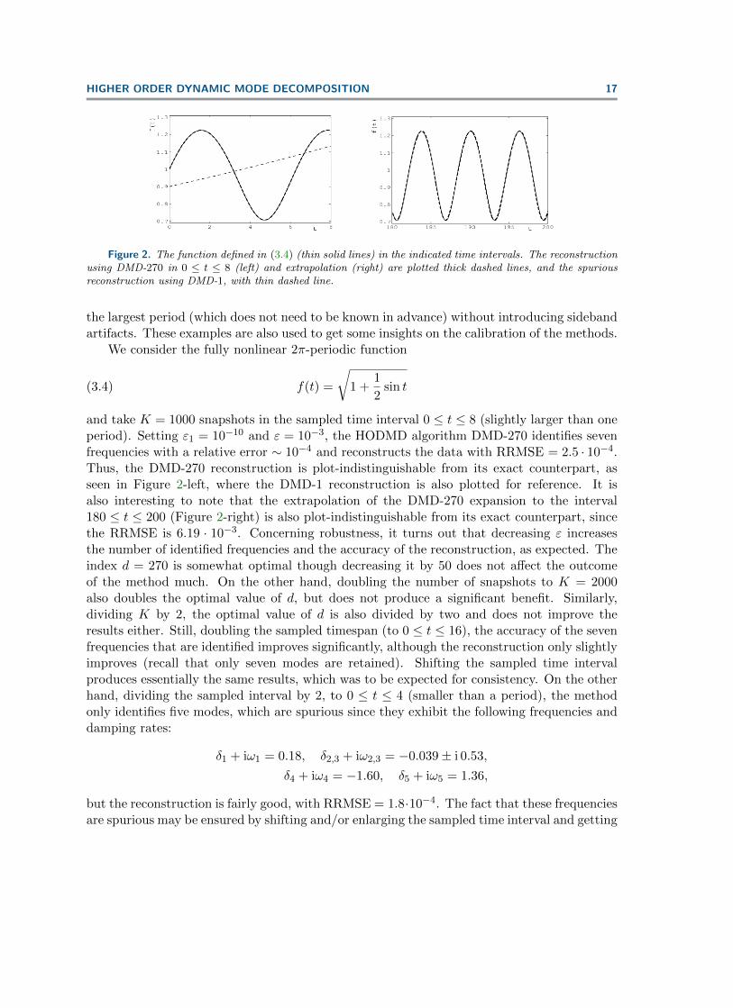
Figure 2. The function defined in (3.4) (thin solid lines) in the indicated time intervals. The reconstructionusing DMD-270 in 0 ≤ t ≤ 8 (left) and extrapolation (right) are plotted thick dashed lines, and the spuriousreconstruction using DMD-1, with thin dashed line.

the largest period (which does not need to be known in advance) without introducing sidebandartifacts. These examples are also used to get some insights on the calibration of the methods.

We consider the fully nonlinear 2π-periodic function

(3.4) f(t) =

√1 +

1

2sin t

and take K = 1000 snapshots in the sampled time interval 0 ≤ t ≤ 8 (slightly larger than oneperiod). Setting ε1 = 10−10 and ε = 10−3, the HODMD algorithm DMD-270 identifies sevenfrequencies with a relative error ∼ 10−4 and reconstructs the data with RRMSE = 2.5 · 10−4.Thus, the DMD-270 reconstruction is plot-indistinguishable from its exact counterpart, asseen in Figure 2-left, where the DMD-1 reconstruction is also plotted for reference. It isalso interesting to note that the extrapolation of the DMD-270 expansion to the interval180 ≤ t ≤ 200 (Figure 2-right) is also plot-indistinguishable from its exact counterpart, sincethe RRMSE is 6.19 · 10−3. Concerning robustness, it turns out that decreasing ε increasesthe number of identified frequencies and the accuracy of the reconstruction, as expected. Theindex d = 270 is somewhat optimal though decreasing it by 50 does not affect the outcomeof the method much. On the other hand, doubling the number of snapshots to K = 2000also doubles the optimal value of d, but does not produce a significant benefit. Similarly,dividing K by 2, the optimal value of d is also divided by two and does not improve theresults either. Still, doubling the sampled timespan (to 0 ≤ t ≤ 16), the accuracy of the sevenfrequencies that are identified improves significantly, although the reconstruction only slightlyimproves (recall that only seven modes are retained). Shifting the sampled time intervalproduces essentially the same results, which was to be expected for consistency. On the otherhand, dividing the sampled interval by 2, to 0 ≤ t ≤ 4 (smaller than a period), the methodonly identifies five modes, which are spurious since they exhibit the following frequencies anddamping rates:

δ1 + iω1 = 0.18, δ2,3 + iω2,3 = −0.039± i 0.53,

δ4 + iω4 = −1.60, δ5 + iω5 = 1.36,

but the reconstruction is fairly good, with RRMSE = 1.8·10−4. The fact that these frequenciesare spurious may be ensured by shifting and/or enlarging the sampled time interval and getting

18 SOLEDAD LE CLAINCHE AND JOSE M. VEGA

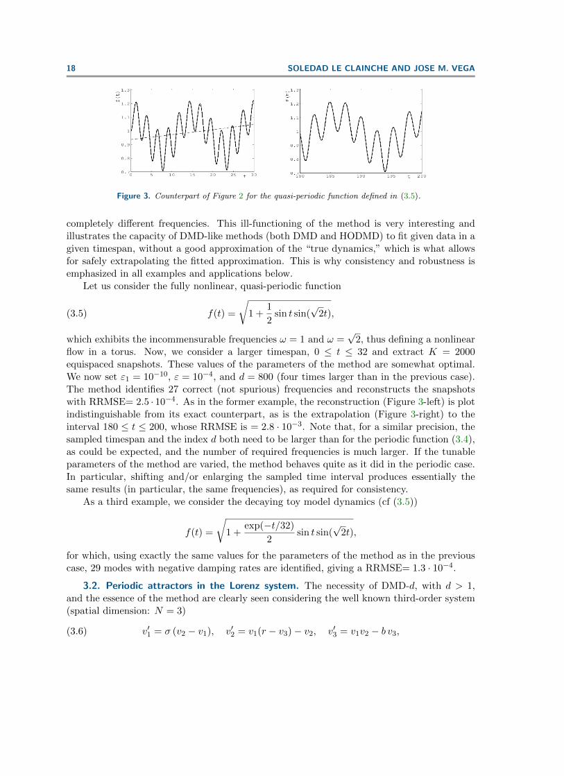
Figure 3. Counterpart of Figure 2 for the quasi-periodic function defined in (3.5).

completely different frequencies. This ill-functioning of the method is very interesting andillustrates the capacity of DMD-like methods (both DMD and HODMD) to fit given data in agiven timespan, without a good approximation of the “true dynamics,” which is what allowsfor safely extrapolating the fitted approximation. This is why consistency and robustness isemphasized in all examples and applications below.

Let us consider the fully nonlinear, quasi-periodic function

(3.5) f(t) =

√1 +

1

2sin t sin(

√2t),

which exhibits the incommensurable frequencies ω = 1 and ω =√

2, thus defining a nonlinearflow in a torus. Now, we consider a larger timespan, 0 ≤ t ≤ 32 and extract K = 2000equispaced snapshots. These values of the parameters of the method are somewhat optimal.We now set ε1 = 10−10, ε = 10−4, and d = 800 (four times larger than in the previous case).The method identifies 27 correct (not spurious) frequencies and reconstructs the snapshotswith RRMSE= 2.5 · 10−4. As in the former example, the reconstruction (Figure 3-left) is plotindistinguishable from its exact counterpart, as is the extrapolation (Figure 3-right) to theinterval 180 ≤ t ≤ 200, whose RRMSE is = 2.8 · 10−3. Note that, for a similar precision, thesampled timespan and the index d both need to be larger than for the periodic function (3.4),as could be expected, and the number of required frequencies is much larger. If the tunableparameters of the method are varied, the method behaves quite as it did in the periodic case.In particular, shifting and/or enlarging the sampled time interval produces essentially thesame results (in particular, the same frequencies), as required for consistency.

As a third example, we consider the decaying toy model dynamics (cf (3.5))

f(t) =

√1 +

exp(−t/32)

2sin t sin(

√2t),

for which, using exactly the same values for the parameters of the method as in the previouscase, 29 modes with negative damping rates are identified, giving a RRMSE= 1.3 · 10−4.

3.2. Periodic attractors in the Lorenz system. The necessity of DMD-d, with d > 1,and the essence of the method are clearly seen considering the well known third-order system(spatial dimension: N = 3)

(3.6) v′1 = σ (v2 − v1), v′2 = v1(r − v3)− v2, v′3 = v1v2 − b v3,

HIGHER ORDER DYNAMIC MODE DECOMPOSITION 19

t20 20.2 20.4 20.6 20.8 21

v1

-60

-40

-20

0

20

40

60

d0 5 10 15 20 25 30

RM

SE

10 -5

10 0

0

5

10

15

20

25

30

35

m

10

0

30

20

Figure 4. The Lorenz system. Left: v1 versus t for the considered periodic orbit (solid), its monochromaticcounterpart (dashed), and the reconstructions using DMD-1 (dotted) and DMD-20 (circles); the vertical line att = 20.6 indicates the upper limit of the sampled interval. Right: RRMSE (as defined in (2.29)) of the DMD-dreconstruction (solid) and the DMD-d extrapolation (dot-dashed), error in the frequency ω (dashed), and thenumber of identified harmonics (dotted line) m versus d. In the right plot, the various errors correspond to theleft scale and the number of identified modes, to the right scale.

first derived by Lorenz [33] as a rough approximation of atmospheric terrestrial convection.As a paradigm of chaos, this system exhibits fairly complex periodic orbits [20], such as thatfor σ = 10, r = 350, and b = 8/3, whose precise representation requires a large numberof harmonics (M � N = 3); see Figure 4-left, where to appreciate the nonmonochromaticcharacter of the orbit, its monochromatic counterpart, a sin(ωt + δ), with appropriate a andδ, is also plotted.

To apply DMD, we integrate (3.6) with initial condition (v1, v2, v3) = (0, 0.1, 0), usingMATLAB “ode45” (with relative and absolute tolerances both equal to = 10−8) and considerK = 60 equispaced snapshots in the interval 20 ≤ t ≤ 20.6, which is comparable to 1.5 timesthe period of the orbit. It is to be noted that the solution in this interval corresponds toa transient behavior, with the dominant mode exhibiting a damping rate δ ∼ 10−2. Thus,identifying the attractor from these snapshots involves extrapolation.

Standard DMD, using the algorithm DMD-1 produces just three modes, which give a poorapproximation (plotted with dotted line in Figure 4-left), while the DMD-d produces a quitegood reconstruction (plotted with circles). After some calibration, the tunable parameters ofthe DMD-d method as set as ε1 = ε = 10−8 for all d, which means that the same threshold,ε1, is used in the SVDs that are needed at steps 1 and 2 of the DMD-d method. Theresulting RMS errors of the reconstructions/extrapolations and the error in the frequencyare as plotted versus d in Figure 4-right; the extrapolation errors are calculated comparingwith the numerical solution in the interval 19990 ≤ t ≤ 20000. Note that DMD-d is fairlyrobust when increasing d. At d = 20, the method identifies m = 35 DMD harmonics and therelative RMS error reaches its minimum at RRMSE ∼ 10−7, which is comparable to both thetolerance of the numerics and the SVD-threshold chosen above (∼ 10−8), meaning that thedecomposition is somewhat optimal. Beyond that value of d, the outcomes worsen, namelythe RRMSE increases and the number of identified frequencies decreases. This is consistentwith the expected behavior as d increases, anticipated in section 2.3.

Additional calculations, not shown here, demonstrate that (as could be expected) main-

20 SOLEDAD LE CLAINCHE AND JOSE M. VEGA

taining the timespan 20 ≤ t ≤ 20.6 but increasing K by a factor (of, say, 10), d must beconsistently increased by the same factor to obtain similar results. And, obviously, increasingthe sampled interval (maintaining both the sampling frequency and d), the method improves.

3.3. On the application to the Stuart–Landau equation. Let us now consider the Stuart–Landau equation [26], which conveniently rescaled is written in terms of a complex amplitudeA as

(3.7) A′ = µ(1 + iν)A− (1 + iβ)|A|2A,

where the bifurcation parameter µ measures departure from the bifurcation point and ν is therescaled detuning. This equation applies in the vicinity of Hopf bifurcation [26] in autonomousdynamical systems. The state vector is approximated as

(3.8) v(t) ' v0 + [V A(t)eiω0t + c.c.],

where higher order harmonics are ignored, V is an eigenvector of the linearized problem atthreshold, and iω0 is the associated eigenvalue. Thus, this equation is relevant at the onset ofvortex shedding in the two-dimensional cylinder wake, considered in this context by Bagheri[5].

Equation (3.7) is solved in closed-form setting

(3.9) A = Reiθ,

which yields

(3.10) R(t) '√µR(0)√

R(0)2 + [µ−R(0)2]e−2µt, θ′(t) = µν − βR(t)2.

It is interesting to note that, even though the Stuart–Landau equation itself is associatedwith weakly nonlinear dynamics in the underlying physical problem, (3.10) represents fullynonlinear dynamics of the Stuart–Landau equation, namely A is not slowly varying. Fort > 1/(2µ), R(t) can be expanded in powers of e−2µt � 1, which requires a large number ofterms if e−2µt is only moderately small. Substituting this expansion into the second expressionin (3.10), integrating in t, and substituting the resulting expansions for R and θ into (3.9) andthe resulting expression for A(t) into (3.8) yields a DMD expansion of the form (1.3), wherethe number of required terms M (namely, the spectral complexity) may be quite large. Thespatial complexity, instead, is N = 3 to the approximation (3.8) (namely, sufficiently closeto the bifurcation point). In other words, standard DMD may not give good descriptions oftransient dynamics near the Hopf bifurcation, and HODMD should be safely used instead.On the other hand, even though the Stuart–Landau equation may also apply beyond the Hopfbifurcation (not close to threshold) in, e.g., the von Karman instability [41], departure fromthe bifurcation point may increase the spatial dimension, which could make the differencebetween standard DMD and HODMD less dramatic.

HIGHER ORDER DYNAMIC MODE DECOMPOSITION 21

4. Application to the CGLE. Let us consider the CGLE for the complex independentvariable u,

∂tu = (1 + iα)∂xxu+ µu− (1 + iβ)|u|2u, with ∂xu = 0 at x = 0, 1,

which depends on the real parameters α and β, which account for dispersion and nonlineardetuning, respectively, and µ, which measures departure from marginal instability and isusually taken as a bifurcation parameter. This equation is invariant under the D1 × SO(2)group generated by the actions x → 1 − x and u → ueic, where c is a constant. Becauseof the stabilizing cubic term, the solutions to this equation are globally bounded, namelyboth u and the spatial derivatives of u are bounded for all t. The CGLE is a well knownparadigm of pattern forming systems that can be considered as a normal form for extendeddissipative systems modeled by partial differential equations near the onset of oscillatoryinstabilities. The equation itself is a simple nonlinear equation that exhibits intrinsicallycomplex dynamics [4], due to the modulational instability if αβ < −1 (Newell’s condition)and µ exceeds a threshold value. It must be noted that as µ increases, the complexity of theattractors does not necessarily increase, as seen in the bifurcations diagram given in Figure 5.Also note that if µ� 1, then the solution must show fast spatio-temporal oscillations becauseof the spatial and temporal steepness scale with

1/√µ and 1/µ,

respectively. For varying µ, the attractors can be periodic, quasi-periodic, and chaotic. Inparticular, the equation exhibits attractors with very large spectral complexity, which are notaccessible to standard DMD. The state variable can be written as

u(x, t) = u0(x, t) eiγt,

where γ can be seen as a (real) frequency shift, which allows for classifying the attractors [55]as follows:

• Type I: Monochromatic, spatially uniform, periodic solutions if u0 is constant.• Type II: Monochromatic, spatially nonuniform, periodic solutions if u0 = u0(x).• Type III: Quasi-periodic solutions if u0 = u0(x, t) is time periodic, with a frequencyω0 incommensurable with γ (which is generically expected).• Type IV: Quasi-periodic solutions, with three involved frequencies if u0 = u0(x, t) is

quasi-periodic, with basic frequencies ω10 and ω2

0, both incommensurable with γ.Thus, type I and II attractors are monochromatic and exhibit just one spatial mode. Intype III attractors, the relevant frequencies are of the form ω = mω0 + γ, for appropriateintegers m, which correspond to the retained frequencies of the periodic function u0 shiftedby the second frequency γ. In type IV attractors, the relevant frequencies are of the formω = m1ω

10 + m2ω

20 + γ, for appropriate integers m1 and m2. Note that in these four cases

|u| = |u0| is (I) steady and spatially uniform, (II) steady and spatially nonuniform, (III) timeperiodic, and (IV) quasi-periodic, respectively.

The attractors of type IV were not considered in [55], where no inexpensive methodto identify these attractors was available. Here, instead, HODMD gives us a very efficient

22 SOLEDAD LE CLAINCHE AND JOSE M. VEGA

means to ascertain the nature of these attractors. On the other hand, the nature of theseattractors will be guessed (not ascertained) below by plotting |u(3/4, t)| versus |u(1/4, t)|. Fora given accuracy, these attractors exhibit finite spectral and spatial complexities and, thus,they can be identified using DMD and HODMD. The CGLE also exhibits chaotic attractors,with finite spatial complexity (for a given accuracy) but arbitrarily large spectral complexity.These attractors cannot be approximated using DMD-like approximations, but they can beidentified as chaotic using these methods, see below.

The snapshots for the various applications of DMD and HODMD below will be numericallycalculated by using a standard Crank–Nicolson plus Adams–Bashforth scheme [14], using atime step ∆t = 10−5 and discretizing spatial derivatives by centered finite differences in auniform grid of 1000 points. The initial condition will be

u =õ (1 + i).

After discarding the transient behavior in 0 ≤ t < t0, the snapshots are calculated in theinterval t0 ≤ t ≤ t1, meaning that we have (t1 − t0)/∆t snapshots at our disposal, but weshall consider a smaller number of snapshots below. Concerning the J spatial points, thesewill all be used in the first set of applications of the DMD-like methods considered in thenext subsection. However, the performance of the HODMD method using a limited numberof spatial points will also be addressed in section 4.2.

4.1. Analysis of the attractors using all spatial data. The snapshots sets will consist ofK-equispaced snapshots in an interval t0 < t < t1, and denoted as

SK[t0,t1].

On the other hand, in order to get comparable results, the thresholds

(4.1) ε1 = 10−8 and ε = 10−6

will be taken in all applications below for the various truncations mentioned in sections 2.1.1–2.1.3 for DMD-1 and in sections 2.2.1–2.2.3 for DMD-d, with d > 1.

Taking the above into account, we now proceed with several representative attractors ofthe CGLE. To begin with, we consider the case

α = −10, β = 10

for various values of µ. The bifurcation diagram for varying µ is given in Figure 5. Asfurther explained in [56], this bifurcation diagram is obtained by plotting |u(3/4, t)| for theintersections of an orbit in the attractor with the Poincare hypersurface

∫ 10 [(1 + iα)∂xxu +

µu − (1 + iβ)|u|2u]u dx = 0. The considered values of α and β mean, since |α| = 10 and|β| = 10 are both large, that the equation is almost conservative (dispersion and nonlineardetuning somewhat large compared to diffusion and nonlinear damping, respectively), namelythe equation is somewhat close to the conservative cubic Schrodinger equation [1], which isfairly demanding from the computational point of view. This case was considered in [56] to

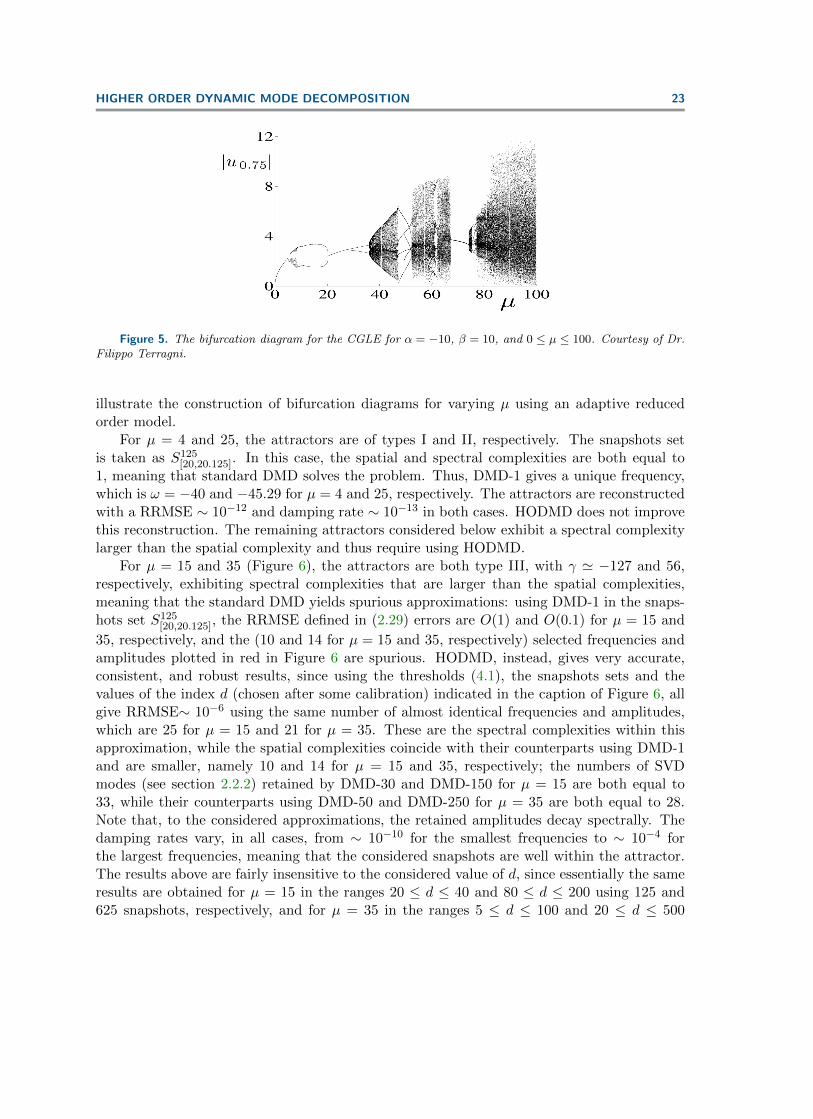
HIGHER ORDER DYNAMIC MODE DECOMPOSITION 23

Figure 5. The bifurcation diagram for the CGLE for α = −10, β = 10, and 0 ≤ µ ≤ 100. Courtesy of Dr.Filippo Terragni.

illustrate the construction of bifurcation diagrams for varying µ using an adaptive reducedorder model.

For µ = 4 and 25, the attractors are of types I and II, respectively. The snapshots setis taken as S125

[20,20.125]. In this case, the spatial and spectral complexities are both equal to1, meaning that standard DMD solves the problem. Thus, DMD-1 gives a unique frequency,which is ω = −40 and −45.29 for µ = 4 and 25, respectively. The attractors are reconstructedwith a RRMSE ∼ 10−12 and damping rate ∼ 10−13 in both cases. HODMD does not improvethis reconstruction. The remaining attractors considered below exhibit a spectral complexitylarger than the spatial complexity and thus require using HODMD.

For µ = 15 and 35 (Figure 6), the attractors are both type III, with γ ' −127 and 56,respectively, exhibiting spectral complexities that are larger than the spatial complexities,meaning that the standard DMD yields spurious approximations: using DMD-1 in the snaps-hots set S125

[20,20.125], the RRMSE defined in (2.29) errors are O(1) and O(0.1) for µ = 15 and

35, respectively, and the (10 and 14 for µ = 15 and 35, respectively) selected frequencies andamplitudes plotted in red in Figure 6 are spurious. HODMD, instead, gives very accurate,consistent, and robust results, since using the thresholds (4.1), the snapshots sets and thevalues of the index d (chosen after some calibration) indicated in the caption of Figure 6, allgive RRMSE∼ 10−6 using the same number of almost identical frequencies and amplitudes,which are 25 for µ = 15 and 21 for µ = 35. These are the spectral complexities within thisapproximation, while the spatial complexities coincide with their counterparts using DMD-1and are smaller, namely 10 and 14 for µ = 15 and 35, respectively; the numbers of SVDmodes (see section 2.2.2) retained by DMD-30 and DMD-150 for µ = 15 are both equal to33, while their counterparts using DMD-50 and DMD-250 for µ = 35 are both equal to 28.Note that, to the considered approximations, the retained amplitudes decay spectrally. Thedamping rates vary, in all cases, from ∼ 10−10 for the smallest frequencies to ∼ 10−4 forthe largest frequencies, meaning that the considered snapshots are well within the attractor.The results above are fairly insensitive to the considered value of d, since essentially the sameresults are obtained for µ = 15 in the ranges 20 ≤ d ≤ 40 and 80 ≤ d ≤ 200 using 125 and625 snapshots, respectively, and for µ = 35 in the ranges 5 ≤ d ≤ 100 and 20 ≤ d ≤ 500

24 SOLEDAD LE CLAINCHE AND JOSE M. VEGA

|u0.25

|0 1 2 3 4

|u0.7

5|

0

0.5

1

1.5

2

2.5

3

3.5

ωm

-1000 -500 0 500 1000

a m

10 -6

10 -4

10 -2

10 0

10 2

|u0.25

|1.5 2 2.5 3 3.5 4

|u0

.75

|

1.5

2

2.5

3

3.5

4

ωm

-3000 -2000 -1000 0 1000 2000 3000

a m

10 -6

10 -4

10 -2

10 0

10 2

Figure 6. The CGLE for α = −10, β = 10, and µ = 15 (top) and 35 (bottom). Left: |u(3/4, t)|versus |u(1/4, t)|. Right: The DMD modes amplitudes am (as calculated in section 2.2.3) versus the associatedfrequencies ωm, as obtained using standard DMD for the whole snapshots set S125

[20,20.125] (red circles) and using

DMD-30 and DMD-50 for µ = 15 and 35, respectively, considering the snapshots sets S125[20,20.125] (black circles),

S125[20.875,21] (black crosses), and DMD-150 and DMD-250 for µ = 15 and 35, respectively, using S625

[20,20.125] (blue

circles) and S625[20.875,21] (blue crosses). Black and blue symbols are plot indistinguishable.

using 125 and 625 snapshots, respectively. Decreasing or increasing d outside these ranges theaccuracy decreases and, in fact, increasing d too much (i.e., d ≥ 500 when 625 snapshots areconsidered), the method diverges.

For µ = 50, the attractor is also type III, with γ ' −150, but more complex than in theformer cases. The counterpart of Figure 6 is given in Figure 7, where it can be seen that,again, standard DMD (red circles), which selects 21 DMD modes, gives completely spuriousresults; as above the RRMSE is O(1). The snapshots sets are indicated in the caption; thesampled timespans are comparable to the period of u0(x, t). Also, to the intended accuracy:

• The lowest sampling frequency (black symbols) is not enough since it only gives con-sistently a part of the relevant frequencies, namely those 65 frequencies with modeamplitudes larger than 10−4. The spatial complexity is 21, the total number of SVDmodes selected by DMD-70 is 141, and the number of retained frequencies is 104.Retaining these 104 modes, the reconstruction shows a RRMSE ∼ 10−6 and plot-indistinguishable amplitudes and frequencies, both using the snapshots sets S250

[20,20.25]

S250[20.75,21] (black circles and crosses, respectively) and the associated values of d indi-

cated in the caption. However, only the first 65 DMD modes correspond to a type IIIsolution since the remaining 104−65 = 39 frequencies would suggest that the solution

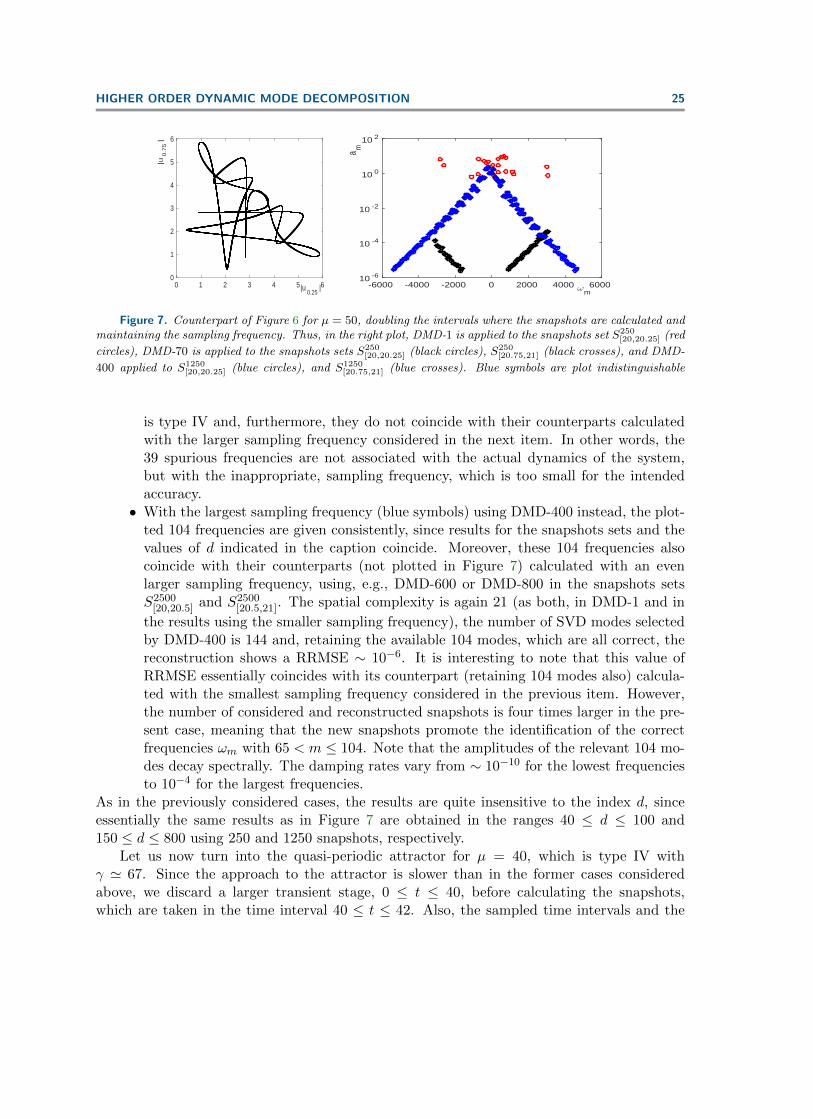
HIGHER ORDER DYNAMIC MODE DECOMPOSITION 25

|u0.25

|0 1 2 3 4 5 6

|u0.7

5|

0

1

2

3

4

5

6

ωm

-6000 -4000 -2000 0 2000 4000 6000

a m

10 -6

10 -4

10 -2

10 0

10 2

Figure 7. Counterpart of Figure 6 for µ = 50, doubling the intervals where the snapshots are calculated andmaintaining the sampling frequency. Thus, in the right plot, DMD-1 is applied to the snapshots set S250

[20,20.25] (red

circles), DMD-70 is applied to the snapshots sets S250[20,20.25] (black circles), S250

[20.75,21] (black crosses), and DMD-

400 applied to S1250[20,20.25] (blue circles), and S1250

[20.75,21] (blue crosses). Blue symbols are plot indistinguishable

is type IV and, furthermore, they do not coincide with their counterparts calculatedwith the larger sampling frequency considered in the next item. In other words, the39 spurious frequencies are not associated with the actual dynamics of the system,but with the inappropriate, sampling frequency, which is too small for the intendedaccuracy.• With the largest sampling frequency (blue symbols) using DMD-400 instead, the plot-

ted 104 frequencies are given consistently, since results for the snapshots sets and thevalues of d indicated in the caption coincide. Moreover, these 104 frequencies alsocoincide with their counterparts (not plotted in Figure 7) calculated with an evenlarger sampling frequency, using, e.g., DMD-600 or DMD-800 in the snapshots setsS2500

[20,20.5] and S2500[20.5,21]. The spatial complexity is again 21 (as both, in DMD-1 and in

the results using the smaller sampling frequency), the number of SVD modes selectedby DMD-400 is 144 and, retaining the available 104 modes, which are all correct, thereconstruction shows a RRMSE ∼ 10−6. It is interesting to note that this value ofRRMSE essentially coincides with its counterpart (retaining 104 modes also) calcula-ted with the smallest sampling frequency considered in the previous item. However,the number of considered and reconstructed snapshots is four times larger in the pre-sent case, meaning that the new snapshots promote the identification of the correctfrequencies ωm with 65 < m ≤ 104. Note that the amplitudes of the relevant 104 mo-des decay spectrally. The damping rates vary from ∼ 10−10 for the lowest frequenciesto 10−4 for the largest frequencies.

As in the previously considered cases, the results are quite insensitive to the index d, sinceessentially the same results as in Figure 7 are obtained in the ranges 40 ≤ d ≤ 100 and150 ≤ d ≤ 800 using 250 and 1250 snapshots, respectively.

Let us now turn into the quasi-periodic attractor for µ = 40, which is type IV withγ ' 67. Since the approach to the attractor is slower than in the former cases consideredabove, we discard a larger transient stage, 0 ≤ t ≤ 40, before calculating the snapshots,which are taken in the time interval 40 ≤ t ≤ 42. Also, the sampled time intervals and the

26 SOLEDAD LE CLAINCHE AND JOSE M. VEGA

|u0.25

|0 1 2 3 4 5

|u0.7

5|

0

1

2

3

4

5

ωm

-4000 -2000 0 2000 4000

a m

10 -6

10 -4

10 -2

10 0

10 2

Figure 8. Counterpart of Figure 7 for µ = 40, with new snapshots sets: in the right plot, DMD-1 is appliedto the snapshots set S1000

[40,41] (red circles), DMD-200 is applied to the snapshots sets S1000[40,41] (black circles),

S1000[41,42] (black crosses), and DMD-1000 applied to S5000

[40,41] (blue circles), and S5000[41,42] (blue crosses).

sampling frequencies are both larger. As a consequence, for the lowest sampling frequency, theconsidered snapshots sets S1000

[40,41] and S1000[41,42] are treated using DMD-200, while S5000

[40,41] and

S5000[41,42] require using DMD-1000. For the intended accuracy (see (4.1)), the spatial complexity

is 18. The counterpart of Figure 7 is given in Figure 8. The results are similar to those obtainedfor the previous cases. As expected, DMD-1 gives a completely spurious solution. Using thesmallest sampling frequency (black symblols) does not solve the problem to the given accuracy.Specifically, the number of SVD modes retained by DMD-200 is 626 and the total number ofretained frequencies, 481; the reconstruction error retaining all modes is RRMSE ∼ 5 · 10−6.However, only the first 157 frequencies (namely, those showing modes amplitudes > 10−4) aredynamically meaningful, as seen comparing with the results obtained from the snapshots setusing the largest sampling frequency (blue symbols). In this case, the number of SVD modesretained by DMD-1000 (larger than with the smaller sampling frequency) is 705 and the totalnumber of retained frequencies is 440 (smaller than with the smaller sampling frequency). Thereconstruction error retaining all modes is RRMSE ∼ 5 · 10−6, comparable to its counterpartusing the smaller sampling frequency, but now the 440 modes are dynamically relevant, whichhas been tested comparing with the results (omitted here) obtained by multiplying both thesampling frequency and the index d by 2. The damping rates vary from ∼ 10−7 for thelowest frequencies to 10−2 for the largest frequencies. Note that, as anticipated, for the samerequired accuracy, the number of relevant frequencies is much larger here than in the periodiccases considered above, as seen comparing the number of blue symbols in Figure 8 with itscounterparts in Figures 6 and 7. As in the formerly considered cases, the results are quiteinsensitive to the index d, since essentially the same results as in Figure 8 are obtained in theranges 180 ≤ d ≤ 300 and 900 ≤ d ≤ 1300 using 1000 and 5000 snapshots, respectively.

Finally, for µ = 7, the attractor is chaotic, which means that the Fourier expansion ofthe orbits are broadband and, moreover, each orbit is unstable. This means that no methodcan be able to produce consistent and robust (i.e., coinciding in shifted sampled intervals)DMD expansions with a finite number of modes, as those obtained above for periodic andquasi-periodic orbits. Namely, the obtained amplitudes and frequencies strongly depend onthe sampled interval because the orbit is chaotic and visits different regions of the attractor

HIGHER ORDER DYNAMIC MODE DECOMPOSITION 27

1 1.5 2 2.5 3 3.50.5

1

1.5

2

2.5

3

3.5

|u0.25

|

|u0.

75|

−600 −400 −200 0 200 400 60010

−6

10−4

10−2

100

102

ωm

a m

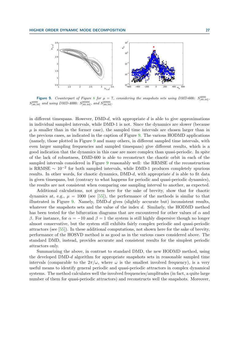
Figure 9. Counterpart of Figure 8 for µ = 7, considering the snapshots sets using DMD-600: S4000[40,44],

S4000[46,50] and using DMD-4000: S20000

[40,44], and S20000[46,50].

in different timespans. However, DMD-d, with appropriate d is able to give approximationsin individual sampled intervals, while DMD-1 is not. Since the dynamics are slower (becauseµ is smaller than in the former case), the sampled time intervals are chosen larger than inthe previous cases, as indicated in the caption of Figure 9. The various HODMD applications(namely, those plotted in Figure 9 and many others, in different sampled time intervals, witheven larger sampling frequencies and sampled timespans) give different results, which is agood indication that the dynamics in this case are more complex than quasi-periodic. In spiteof the lack of robustness, DMD-600 is able to reconstruct the chaotic orbit in each of thesampled intervals considered in Figure 9 reasonably well: the RRMSE of the reconstructionis RRMSE ∼ 10−2 for both sampled intervals, while DMD-1 produces completely spuriousresults. In other words, for chaotic dynamics, DMD-d, with appropriate d is able to fit datain given timespans, but (contrary to what happens for periodic and quasi-periodic dynamics),the results are not consistent when comparing one sampling interval to another, as expected.

Additional calculations, not given here for the sake of brevity, show that for chaoticdynamics at, e.g., µ = 1000 (see [55]), the performance of the methods is similar to thatillustrated in Figure 9. Namely, DMD-d gives (slightly accurate but) inconsistent results,whatever the snapshots sets and the value of the index d. Similarly, the HODMD methodhas been tested for the bifurcation diagrams that are encountered for other values of α andβ. For instance, for α = −10 and β = 1 the system is still highly dispersive though no longeralmost conservative, but the system still exhibits fairly complex periodic and quasi-periodicattractors (see [55]). In these additional computations, not shown here for the sake of brevity,performance of the HOSVD method is as good as in the various cases considered above. Thestandard DMD, instead, provides accurate and consistent results for the simplest periodicattractors only.

Summarizing the above, in contrast to standard DMD, the new HODMD method, usingthe developed DMD-d algorithm for appropriate snapshots sets in reasonable sampled timeintervals (comparable to the 2π/ω, where ω is the smallest involved frequency), is a veryuseful means to identify general periodic and quasi-periodic attractors in complex dynamicalsystems. The method calculates well the involved frequencies/amplitudes (in fact, a quite largenumber of them for quasi-periodic attractors) and reconstructs well the snapshots. Moreover,

28 SOLEDAD LE CLAINCHE AND JOSE M. VEGA

the dynamically relevant modes are identified by comparing the obtained results using varioussnapshot sets. It must be noted that, since we had a very large number of snapshots atour disposal (from the numerical computations) no attempt has been made to minimize thesnapshots number, K. Instead, we have taken K sufficiently large to reconstruct the solutionwith RRMSE ∼ 10−6, which has required identifying fairly large frequencies. If, instead, onlya RRMS ∼ 10−3 were sought, then the required numbers of snapshots in Figure 6 would havebeen 85 with d = 5 (instead of 125 with d = 30) and 25 with d = 5 (instead of 125 withd = 50) for µ = 15 and 35, respectively. Similarly, the numbers of snapshots in Figures 7and 8 would have been 140 with d = 10 (instead of 250 with d = 70) and 700 with d = 100(instead of 1000 with d = 200), respectively. On the other hand, chaotic attractors can beidentified from the ill-functioning of the method. As done for the Lorenz system in section3.2, decaying dynamics may be used to identify the large time attractors via extrapolation,but this application has not been illustrated in this section for the sake of brevity.

4.2. Recovering the relevant modes amplitudes and frequencies using a limited amountof noisy data. As anticipated in the introduction and illustrated in some toy-model examplesin section 3.1, the HODMD algorithm DMD-d, with appropriate d, takes full advantage ofboth the spatial and temporal redundancies in periodic and quasi-periodic dynamics of thetype

(4.2) v 'M∑m=1

amumeiωmt,

which has a potential interest to do the following:• Recover the relevant mode amplitudes and frequencies using a limited amount of spa-

tial data.• Filter out small errors.

On the other hand, as DMD-1 applied to time periodic and quasi-periodic flows is relatedto FFT [18], DMD-d can be compared to PSD [39], where the number of segments used inPSD is the counterpart of the index d in the DMD-d algorithm. All these are the object ofthe present section. For the sake of brevity, to avoid defining a new dynamical system, thisillustration relies in the CGLE considered in this section.

Before proceeding further, some remarks are in order:• When comparing results obtained using different numbers of spatial points, comparison

of the relevant frequencies is straightforward, but comparison of the mode amplitudesis more tricky. Scaling the modes um appearing in (4.2) as we have done in thispaper (see (2.12)), namely such that ‖um‖ =

√J , where J is the spatial dimension

of the given data, makes the mode amplitudes am as independent as possible from J .However, when comparing data from two quite different values of J (e.g., J = 1000and 1), the two sets of amplitudes will only coincide if the data is spatially uniform.Otherwise, only the frequencies can be safely compared.• For J = 1, the scaling (2.29) yields ‖um‖ = 1, namely the mode amplitudes exactly

coincide with their counterparts in PSD and FFT calculations.• After some calibration for the CGLE, it has been found that HODMD also recovers

the mode amplitudes if the considered number of spatial data is comparable to the

HIGHER ORDER DYNAMIC MODE DECOMPOSITION 29

spatial complexity.• The following advantages of HODMD can be anticipated in periodic dynamics:

– As illustrated in the last section, HODMD gives good results in arbirary sam-pled time intervals whose length is comparable to the period. FFT and PSD,instead, produce artifacts unless the sampled timespan either is sufficientlylarge or coincides with the period.

– For slightly decaying dynamics, HODMD identifies both the frequencies andthe (small) damping rates, which in principle gives good reconstructions wit-hout any additional treatment. Moreover, setting to zero the damping ratesproduces a good approximation of the final attractors. Instead, the nonzerodamping rates produce undesirable sideband artifacts when using FFT andPSD.

These two observations are even more evident when treating quasi-periodic dynamics.In what follows, several cases will be considered in which the following calculations will

be compared:• DMD-d-full: DMD-d calculations using all spatial data (as already done in the last

section). These will be taken as reference.• DMD-d-N : DMD-d calculations using a number of spatial points equal to the spatial

complexity.• DMD-d-1: DMD-d calculations using just one spatial point, namely x = 1/4.• PSD-d: PSD calculations using d segments (and just one spatial point).• FFT: FFT calculations (for just one spatial point).

It must be noted that the mode amplitudes appearing in the DMD-expansions involvingdifferent spatial points need not coincide because the spatial modes are generally different.In the application of DMD-d to the various cases below, the index d will be taken as thatcalibrated in the last section. The HODMD thresholds will also be taken identical to thoseused in the last section, namely as defined in (4.1). The same threshold ε = 10−6 will also beused for PSD and FFT truncation.

To begin with, we address the case α = −10, β = 10, and µ = 15, already consideredin Figure 6. The results applying the five methods indicated above are depicted in Figure10. As can be seen in this figure, DMD-150-full, DMD-150-10 (note that 10 is the spatialcomplexity), and DMD-500-1 all give very similar results, since the identified frequenciescoincide though, as anticipated there are some differences in the associated mode amplitudes.In fact, both, DMD-150-10 and DMD-500-1 (with the sampled timespan doubled) correctlyidentify the 25 and 24 relevant (to the given accuracy) frequencies, respectively. On the otherhand, the results are very insensitive to the index d since, e.g., DMD-d-1, with 450 ≤ d ≤ 800yields essentially the same result as that plotted in Figure 10. Instead, both PSD and FFTonly approximately identify the first 20 frequencies, which, moreover, do not show the largestamplitudes. This is in spite of the fact that the sampled time interval used by DMD-500-1has been multiplied by 240 and 720 for PSD and FFT, respectively (because using the samesampled interval as when using DMD-500-1, the results are completely spurious).

The ill-functioning of both FFT and PSD is due to the artifacts introduced by thesemethods when the sampled interval is not commensurable with the period of the solution. Byits own nature, these artifacts are not present in HODMD (and neither in standard DMD when

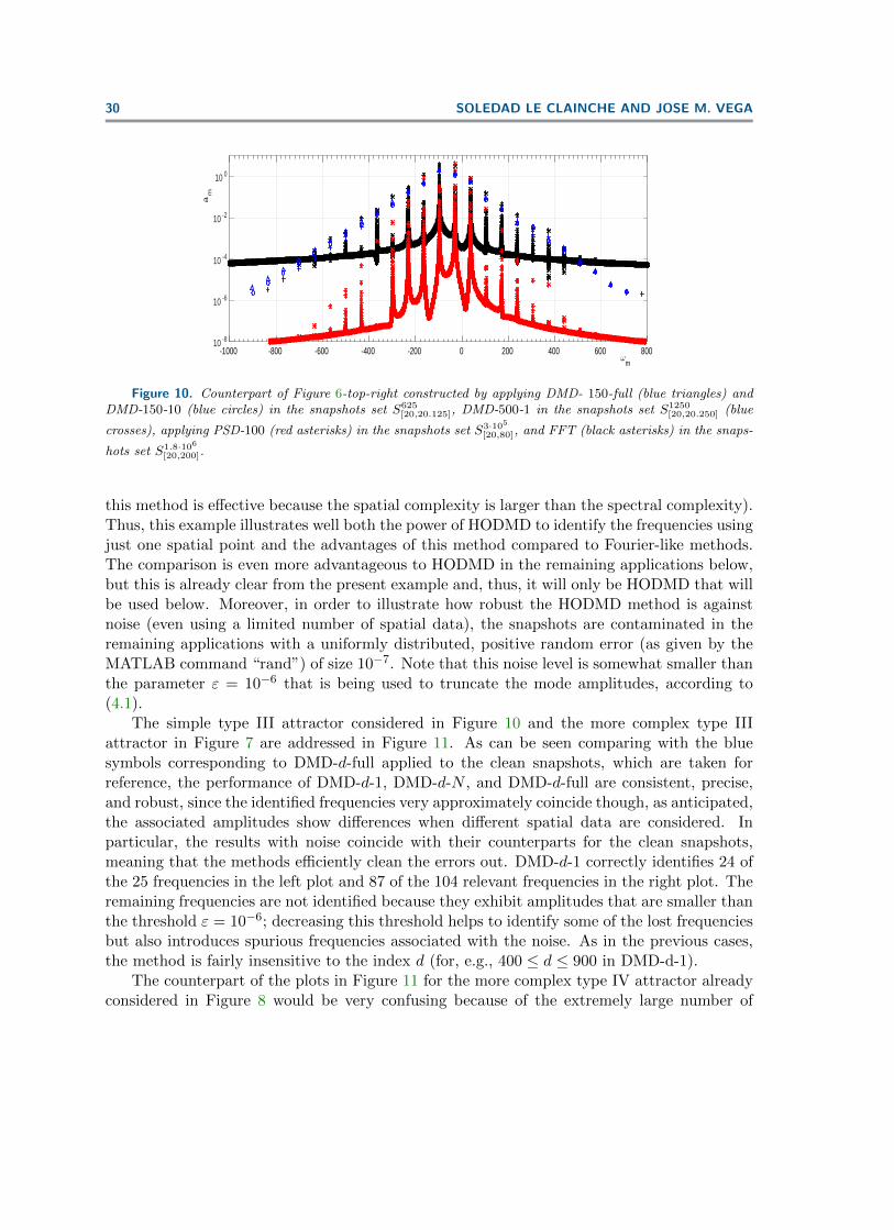
30 SOLEDAD LE CLAINCHE AND JOSE M. VEGA

ωm

-1000 -800 -600 -400 -200 0 200 400 600 800

am

10 -8

10 -6

10 -4

10 -2

10 0

Figure 10. Counterpart of Figure 6-top-right constructed by applying DMD- 150-full (blue triangles) andDMD-150-10 (blue circles) in the snapshots set S625

[20,20.125], DMD-500-1 in the snapshots set S1250[20,20.250] (blue

crosses), applying PSD-100 (red asterisks) in the snapshots set S3·105[20,80], and FFT (black asterisks) in the snaps-

hots set S1.8·106[20,200].

this method is effective because the spatial complexity is larger than the spectral complexity).Thus, this example illustrates well both the power of HODMD to identify the frequencies usingjust one spatial point and the advantages of this method compared to Fourier-like methods.The comparison is even more advantageous to HODMD in the remaining applications below,but this is already clear from the present example and, thus, it will only be HODMD that willbe used below. Moreover, in order to illustrate how robust the HODMD method is againstnoise (even using a limited number of spatial data), the snapshots are contaminated in theremaining applications with a uniformly distributed, positive random error (as given by theMATLAB command “rand”) of size 10−7. Note that this noise level is somewhat smaller thanthe parameter ε = 10−6 that is being used to truncate the mode amplitudes, according to(4.1).

The simple type III attractor considered in Figure 10 and the more complex type IIIattractor in Figure 7 are addressed in Figure 11. As can be seen comparing with the bluesymbols corresponding to DMD-d-full applied to the clean snapshots, which are taken forreference, the performance of DMD-d-1, DMD-d-N , and DMD-d-full are consistent, precise,and robust, since the identified frequencies very approximately coincide though, as anticipated,the associated amplitudes show differences when different spatial data are considered. Inparticular, the results with noise coincide with their counterparts for the clean snapshots,meaning that the methods efficiently clean the errors out. DMD-d-1 correctly identifies 24 ofthe 25 frequencies in the left plot and 87 of the 104 relevant frequencies in the right plot. Theremaining frequencies are not identified because they exhibit amplitudes that are smaller thanthe threshold ε = 10−6; decreasing this threshold helps to identify some of the lost frequenciesbut also introduces spurious frequencies associated with the noise. As in the previous cases,the method is fairly insensitive to the index d (for, e.g., 400 ≤ d ≤ 900 in DMD-d-1).

The counterpart of the plots in Figure 11 for the more complex type IV attractor alreadyconsidered in Figure 8 would be very confusing because of the extremely large number of

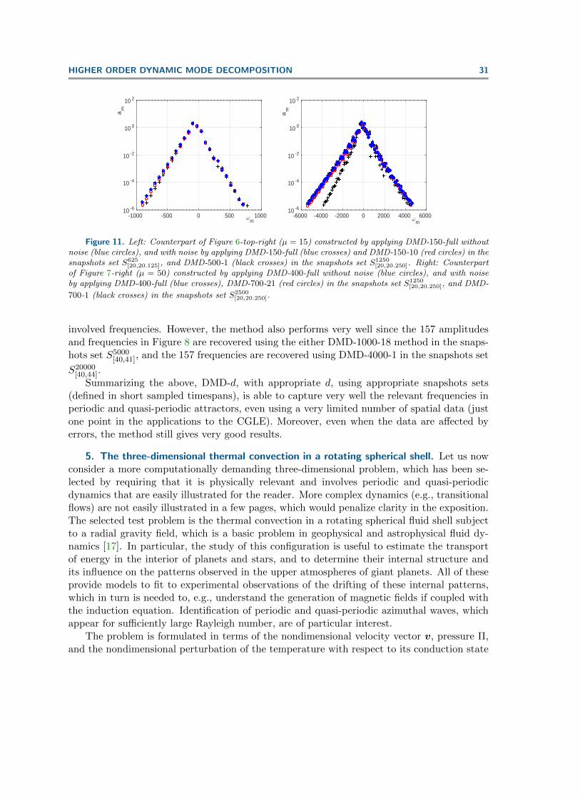
HIGHER ORDER DYNAMIC MODE DECOMPOSITION 31

ωm

-1000 -500 0 500 1000

am

10 -6

10 -4

10 -2

10 0

10 2

ωm

-6000 -4000 -2000 0 2000 4000 6000

am

10 -6

10 -4

10 -2

10 0

10 2

Figure 11. Left: Counterpart of Figure 6-top-right (µ = 15) constructed by applying DMD-150-full withoutnoise (blue circles), and with noise by applying DMD-150-full (blue crosses) and DMD-150-10 (red circles) in thesnapshots set S625

[20,20.125], and DMD-500-1 (black crosses) in the snapshots set S1250[20,20.250]. Right: Counterpart

of Figure 7-right (µ = 50) constructed by applying DMD-400-full without noise (blue circles), and with noiseby applying DMD-400-full (blue crosses), DMD-700-21 (red circles) in the snapshots set S1250

[20,20.250], and DMD-

700-1 (black crosses) in the snapshots set S2500[20,20.250].

involved frequencies. However, the method also performs very well since the 157 amplitudesand frequencies in Figure 8 are recovered using the either DMD-1000-18 method in the snaps-hots set S5000

[40,41], and the 157 frequencies are recovered using DMD-4000-1 in the snapshots set

S20000[40,44].

Summarizing the above, DMD-d, with appropriate d, using appropriate snapshots sets(defined in short sampled timespans), is able to capture very well the relevant frequencies inperiodic and quasi-periodic attractors, even using a very limited number of spatial data (justone point in the applications to the CGLE). Moreover, even when the data are affected byerrors, the method still gives very good results.

5. The three-dimensional thermal convection in a rotating spherical shell. Let us nowconsider a more computationally demanding three-dimensional problem, which has been se-lected by requiring that it is physically relevant and involves periodic and quasi-periodicdynamics that are easily illustrated for the reader. More complex dynamics (e.g., transitionalflows) are not easily illustrated in a few pages, which would penalize clarity in the exposition.The selected test problem is the thermal convection in a rotating spherical fluid shell subjectto a radial gravity field, which is a basic problem in geophysical and astrophysical fluid dy-namics [17]. In particular, the study of this configuration is useful to estimate the transportof energy in the interior of planets and stars, and to determine their internal structure andits influence on the patterns observed in the upper atmospheres of giant planets. All of theseprovide models to fit to experimental observations of the drifting of these internal patterns,which in turn is needed to, e.g., understand the generation of magnetic fields if coupled withthe induction equation. Identification of periodic and quasi-periodic azimuthal waves, whichappear for sufficiently large Rayleigh number, are of particular interest.

The problem is formulated in terms of the nondimensional velocity vector v, pressure Π,and the nondimensional perturbation of the temperature with respect to its conduction state

32 SOLEDAD LE CLAINCHE AND JOSE M. VEGA

profile, Θ. The units of length, time, temperature, and pressure for nondimensionalizationare d, d2/ν, ν2/(αγd4), and ρ0ν

2/d, respectively, were d = r∗o − r∗i is the difference betweenthe (dimensional) outer and inner radii, ν is the kinematic viscosity, γr∗i is the imposed radialgravity at the inner radius, α is the thermal expansion coefficient, and ρ0 is the density atthe reference temperature. Using a rotating Cartesian coordinate frame, with origin at thecommon center of the inner and outer spheres, with the z axis along the rotation axis, thenondimensional continuity, momentum, and energy equations governing the dynamics of thefluid in the Boussinesq approximation are

∇ · v = 0,

∂tv + (v · ∇)v + 2E−1k× v = −∇Π +∇2v + Θr,

σ(∂tΘ + v · ∇Θ) = ∇2Θ + Rη(1− η)−2r−3r · v,

where k is the vertical unit vector, r = (x,y, z), η = r∗i /r∗o is the inner to outer radii ratio,

σ = ν/κ is the Prandtl number (with κ = thermal conductivity), E = ν/(ωd2) is the Eckmannumber, and R = γα∆Td4/(νκ) is the Rayleigh number. The boundary conditions arehomogeneous Dirichlet at both the inner and outer spheres. For nonzero rotation, the resultingproblem is invariant under the symmetry group SO(2)×Z2, generated by the rotations aboutthe vertical z axis and the up-down reflection with respect to the equatorial plane. Invarianceunder rotation is essential to obtain rotating waves, most of which are also (instantaneously)invariant under the up/down symmetry.

For convenience, the pressure and the continuity equation are both eliminated from theformulation by taking the curl of the momentum equation and writing the (solenoidal) velocityfield as

v = ∇× (Ψr) +∇×∇× (Φr),

where Ψ and Φ are the toroidal and poloidal scalar potentials, respectively, first introduced byChandrasekhar [15]. The resulting problem is written in spherical coordinates (r, θ, φ), whereθ and φ are the colatitude and longitude, respectively, in the rotating frame of referencelinked to the spherical shell. The non-dimensional temperature and the scalar potentials areexpanded in spherical harmonics, and spatially discretized using Gauss–Lobatto collocation(with 25 × 64 × 128 collocation points in (r, θ, φ)). Several fairly subtle ingredients are usedfor dealiasing and, especially, for continuation along the periodic and quasi-periodic branches;see [23, 47] and references therein for further details.

The results considered below are concerned with the case σ = 0.1 and E = 10−4, whichsomehow corresponds to the outer atmosphere of some planets such as Jupiter. It turns outthat, for the outer/inner radii ratio η in the range 0.32 ≤ η ≤ 0.35, the system exhibits a fairlycomplex bifurcation diagram, which is quite efficiently calculated in [46] using continuation,not only of periodic orbits but also of invariant tori (a fairly demanding problem). Generically,the purely conductive state (nonuniform temperature distribution, with no convection) losesstability in a Hopf bifurcation, where a new branch of periodic solutions is born, which is apure rotating wave (namely, a steady pattern in reference frame which is rotating in the alreadyconsidered rotating frame linked to the spherical shell). An example is given in Figure 12 that

HIGHER ORDER DYNAMIC MODE DECOMPOSITION 33

Figure 12. Sketch of a snapshot showing the contour levels of Θ in an intermediate spherical surface (left),the equatorial plane (middle), and a meridian plane (right); courtesy of Professor Marta Net. The plottedsnapshot is rigidly rotating in the azimuthal direction. The horizontal segment plotted with thick solid line inthe right plot corresponds to the 15% outer part of the radial equatorial segment, which will be used in Figure13.

shows an azimuthal wavenumber m = 8 and is rigidly rotating in the azimuthal direction witha velocity c, meaning that the frequency of the associated periodic pattern is ω = c/8. In otherwords, concentrating for simplicity in the temperature field, the spatio-temporal structure ofthe pattern is given by

(5.1) Θ(r, θ, φ, t) =N∑n=1

Θn(r, θ)ein(ωt−8φ) + c.c.,

which can be seen as the relevant DMD-expansion.There are several branches of rotating waves, exhibiting different azimuthal wave-numbers

m in the range 3 ≤ m ≤ 8, which bifurcate from the conduction states at different criticalRayleigh numbers, R ∼ 105. Some of these solution branches are stable but lose stability viaNeimark–Sacker bifurcations (complex Floquet multipliers; see [26]) that produce invarianttori (quasi-periodic solutions). On the other hand, for some critical values of η, two of theperiodic branches coalesce, namely the bifurcation points associated with two different valuesof m occur at the same critical Rayleigh number, giving a (codimension-two) double Hopfbifurcation that also produces invariant tori. For instance, at ηc = 0.33079 and Rc = 2.0069 ·105, a double Hopf bifurcation [26] takes place that involves the m = 5 and 6 modes; see [46]for further details.

The cases analyzed in this article are two representative stable flows, one periodic andanother quasi-periodic. The spatio-temporal data that will be used for both have been provi-ded to us by Professors Joan Sanchez and Marta Net, who obtained them using the algorithmoutlined above. Both flows are symmetric with respect to the meridional plane. Consequently,DMD-d has been applied only to half of the three-dimensional domain (positive colatitudeθ ≥ 0). For simplicity in the presentation, only the thermal field, Θ(r, θ, φ, t) will be consideredbelow, both in the performed DMD computations and in all illustrations.

The considered periodic flow is the purely rotating wave illustrated in Figure 12, whichcorresponds to R = 8 · 105 and shows that such flow is steady in a rotating (with the phasevelocity) reference frame. Such steady flow, in turn, is periodic in the azimuthal direction,with a fundamental wavenumber equal to 8. Therefore, this is of the form (5.1), where N

34 SOLEDAD LE CLAINCHE AND JOSE M. VEGA

Figure 13. Mode amplitude (right) versus the frequency for the modes obtained by applying DMD-1 (redcrosses) and DMD-40 (blue circles) to a set of 100 equispaced snapshots, with a nondimensional time shiftbetween snapshots equal to 2.766 · 10−3, considering the meridian plane φ = 0 (left) and the 85% outer part ofthe radial line φ = ϕ = 0 (right).

is the number of modes to be retained and ω = 45.3354 is the fundamental frequency. Thetemporal structure of this three-dimensional flow is fairly simple and, moreover, the spatialand temporal complexities of the associatd DMD expansion are both equal to the numberof retained frequencies, N . This is because, due to the factor e−8inφ, the spatial modesΘn(r, θ)e−8inφ are obviously linearly independent (in fact, they are pairwise orthogonal withthe usual L2 inner product). Consequently, as emphasized in the paper, the advantagesof HODMD with respect to the standard DMD method are very weak in the whole three-dimensional flow. In fact, retaining the mean flow and the four most energetic oscillatorymodes, both DMD-40 and DMD-1 give relative RMS errors RRMSE ∼ 10−5, comparable tothe truncation errors in the numerical scheme. Restricting to the meridian plane θ = 0, therestricted DMD expansion is (cf. (5.1))

(5.2) Θ(r, θ, 0, t) =

N∑n=1

Θn(r, θ)einωt + c.c., with rin ≤ r ≤ rout, 0 ≤ θ ≤ π/2.

Using the restricted snapshots, the plots of the amplitudes versus the frequencies computedby DMD-1 and DMD-40 are both very good and still plot indistinguishable, as seen in Figure13-left, though DMD-40 slightly outperforms DMD-1, since the relative errors of the frequencyof the fourth harmonic (comparing with the three-dimensional computations) are ∼ 10−6 and∼ 10−3, respectively. The advantages of using delayed snapshots are appreciated by drasticallyreducing the number and quality of the observables. This is seen by considering only the lastsix Gauss–Lobatto collocation points in the radial line θ = φ = 0, which corresponds to theouter 15% segment of this radial (plotted with a thick solid line in the right plot in Figure12) and yields the restricted DMD expansion (cf. (5.1)–(5.2))

(5.3) Θ(r, 0, 0, t) =N∑n=1

Θn(r)einωt + c.c., with 0.85 ≤ r − rin ≤ rout − rin(= 1).

Note in Figure 12-right that the thermal activity in this small segment of the radial line is verysmall. In spite of this, DMD-40 (see Figure 13-right) is still able to identify the mean flow and

HIGHER ORDER DYNAMIC MODE DECOMPOSITION 35

Table 1Wavenumbers n1 and n2 and frequencies, as defined in (5.5), for the 12 most energetic modes in the quasi-

periodic attractor considering the whole amount of three-dimensional data (3D), the meridian plane θ = 0 (2D),and the line φ = θ = 0 (1D), as calculated by applying DMD-200 and DMD-1, as indicated.

3D 2D 1D

DMD-200 DMD-200 DMD-1 DMD-200 DMD-1

n1 n2 ω

0 0 0.0000 0.0000 0.0000 0.0000 0.0000

1 0 47.5890 47.5890 47.9306 47.5891 55.6587

0 1 239.8411 239.8412 240.8474 239.8408 −−1 1 192.2520 192.2535 192.9154 192.2524 187.5543

2 0 95.1783 95.1744 96.0682 95.1749 −1 1 287.4301 287.4285 287.7189 287.4288 280.4798

2 1 335.0192 335.0139 344.1997 335.0210 −0 2 479.6822 479.6717 − 479.6807 −−2 1 144.6444 144.1315 − 143.8763 −−1 2 432.0838 432.0914 − 432.0938 −1 2 527.2712 527.1714 − 527.2698 −3 0 142.7519 142.4148 124.5031 144.9524 −3 1 382.7911 382.4096 − 382.9238 351.8692

three oscillating modes and reconstruct the restricted snapshots with a relative RMS errorRRMSE∼ 10−5; also, DMD-40 the relative errors in the three identified frequencies is ∼ 10−4.The fourth oscillating mode exhibits a too small amplitude in this restricted segment, smallerthan truncation errors in the numerical approximation, and cannot be identified. The verygood identification of the frequencies and the very small reconstruction error clearly illustratethe advantages of using the delayed snapshots. DMD-1, instead, only recognizes the meanflow and the first harmonic.

Let us now consider the quasi-periodic attractor that is obtained for R = 1.1 · 106. Thisattractor can be seen as resulting from the nonlinear interaction of two purely rotating waves,with wavenumbers m = 6 and m = 8. Thus, the counterpart of (5.1) is

(5.4) Θ(r, θ, φ, t) =∑n1,n2

Θn1n2(r, θ)ei[n1(ω1t−8φ)+n2(ω2t−6φ)] + c.c.,

for some (incommensurable) fundamental frequencies ω1 and ω2; the sum is extended toa number of retained pairs of values of the integers n1 and n2. As in the periodic case, thefactor e−i(−(8n1+6n2)φ makes the spatial modes fairly uncorrelated, which means that using thewhole amount of three-dimensional data, retaining a reasonable number of modes, HODMDis not expected to dramatically outperform standard DMD. However, it is interesting tonote that both DMD-1 and DMD-200 (applied to a set of 500 equispaced snapshots, with anondimensional time-shift between snapshots equal to 5 · 10−4) are able to identify quite wellthe fundamental frequencies and the harmonics, defined as

(5.5) ω = n1ω1 + n2ω2,

which are displayed in Table 1 (third column) and will be used for reference below. As can

36 SOLEDAD LE CLAINCHE AND JOSE M. VEGA

Figure 14. Counterpart of Figure 13 for the quasi-periodic attractor.

be checked by the reader, these frequencies satisfy quite well the commensurability relation(5.5).

As in the periodic case, restricting to the meridian plane θ = 0 and the radial line θ =φ = 0, namely restricting (5.4) to

Θ(r, θ, 0, t) =∑n1,n2

Θn1n2(r, θ)ei(n1ω1t+n2ω2)t + c.c.,

in rin ≤ r ≤ rout, 0 ≤ θ ≤ π/2 and

Θ(r, 0, 0, t) =∑n1,n2

Θn1n2(r)ei(n1ω1+n2ω2)t + c.c. with rin ≤ r ≤ rout,

respectively, decreases the spatial complexity. In particular, restricting to the meridian planeθ = 0, Table 1 and Figure 14 show that while DMD-200 identifies all frequencies and re-constructs the snapshots with great precision (RRMSE ∼ 10−3); DMD-1 gives much worseresults, since the reconstruction involves a larger error (RRMSE ∼ 10−2) and the frequenciesare identified with an error that increases as the amplitude of the mode decreases. More-over, restricting to the radial line φ = θ = 0, DMD-1 gives completely spurious results inconnection with both the identified frequencies (see Table 1) and the reconstruction (RRMSE∼ 0.4), but DMD-200 approximates the considered modes with a reasonable accuracy, sinceRRMSE ∼ 10−3 and the frequencies are well identified (see Table 1). Thus, the advantagesof using delayed snapshots are clearly seen, for a given spectral complexity, as the number ofobservables (and thus the spatial complexity) is decreased.

Finally, the mean flow and the spatial modes associated with the two fundamental fre-quencies are considered in Figure 15. As can be seen:

• The thermal activity mainly concentrates (for both the mean flow and the fundamentalmodes) near the equator and also somewhat near the inner boundary of the sphericalshell for the 10-mode and 20-mode, but in more interior regions for both the meanflow and the remaining two oscillatory modes.• The real and imaginary parts of the oscillatory modes are not proportional to each ot-

her, meaning that these modes are not standing but progressive, namely the associatedactivity oscillates back and forth in the meridian plane.

HIGHER ORDER DYNAMIC MODE DECOMPOSITION 37

Mean flow <(Θ10) =(Θ10) <(Θ01) =(Θ01)

<(Θ−11) =(Θ−11) <(Θ20) =(Θ20)

Figure 15. The five most energetic modes obtained for the quasi-periodic attractor in the meridian planeθ = 0, via DMD-200, considering the mean flow, and the real and imaginary parts of the oscillatory modesassociated with the two fundamental frequencies.

Summarizing, as anticipated, the considered dynamics is (on purpose) somewhat simple,even in the quasi-periodic case, where the various DMD-modes are associated with purelyrotating waves, whose three-dimensional spatial structures are fairly uncorrelated (see (5.1)and (5.4)). Thus, the advantages of using delayed snapshots are not appreciated when thewhole amount of three-dimensional data is used. However, as the data used is restrictedto the meridian plane and a radial line in the equatorial plane, the advantages of usingHODMD become clear. This is relevant keeping in mind the identification of the spatio-temporal structures using a limited number of observables in the applications outlined at thebeginning of this section. Obviously, as it happened with the CGLE considered in section 4,delayed snapshots are unavoidable in the analysis of fluid flows involving a larger temporalcomplexity (and noise, when dealing with experimental data), but the analysis and descriptionof these flows is more involved and well beyond the scope of this paper.

6. Concluding remarks. A new HODMD method has been developed that generalizesstandard DMD by using the standard method with time-lagged snapshots. An algorithmlabeled as DMD-d, where d ≥ 1 indicates the number of involved time-delayed snapshots, hasbeen derived that permits calculating the new decomposition in a robust and precise way.

The simplest algorithm, DMD-1, is very similar to the original DMD method developed bySchmid [48]. There is a conceptual difference between both, however, since DMD-1 separatescalculations in two steps: the first SVD application to the whole snapshot matrix involves thespatial truncation, which defines from the outset the spatial modes, the spatial complexity N ,and the reduced snapshots. The latter are used in the second step to calculate a DMD de-

38 SOLEDAD LE CLAINCHE AND JOSE M. VEGA

composition for the reduced snapshots, which is readily translated into a DMD decompositionof the original snapshots by using the spatial modes.

For d > 1, the DMD-d algorithm is conceptually new and able to cope with cases (notaccessible to standard DMD) in which the DMD-modes associated with different frequen-cies/growth rates are linearly dependent. The DMD-d algorithm turns out to be quite robustin connection with varying d. Since, after identification of the temporal modes, the applicationof DMD-d with large d is computationally inexpensive, a good strategy is to apply DMD-1and DMD-d for several sample values of d and compare results to guess the appropriate valueof d.

The new method has been illustrated and tested in several toy models, the Stuart–Landauequation, the Lorenz system, and the CGLE. In particular, in the applications to noisy toymodels, it has been proven that the new HODMD method is much more precise and robustthan standard DMD in the presence of noise.

For a periodic attractor in the Lorenz system involving a large number of harmonics, thenew HODMD method quite efficiently identifies the correct basic frequency of the periodicsolution and the amplitude of the harmonics. In addition, using the method in transientdynamics approaching the periodic attractor, the method is able to efficiently extrapolate tothe final attractor.

Concerning the CGLE considered in section 4, a battery of representative periodic andquasi-periodic attractors has been considered. Except for trivial cases (namely, the attractorslabeled as type I and II in section 4), the standard DMD gives spurious results but the newmethod correctly identifies the relevant frequencies and amplitudes to the precision that isbeing sought. In addition, the method has been used to recover the relevant frequenciesconsidering a limited number of grid points, both for the clean databases and after addingrandom noise. Again, the method performs quite well since, in particular, applying the methodwith just one grid point, the results are much better than using FFT and PSD.

Concerning the more computationally demanding problem describing thermal convectionin a rotating spherical shell considered in section 5, the advantages of using the delayedsnapshots in the HODMD method have been illustrated in two representative attractors of thesystem, namely one periodic consisting in a purely rotating wave, and another quasi-periodicinvolving the nonlinear interaction between two rotating waves. Even though no intentionwas made to deal with actual observational data (which bears its own difficulties due to theunavoidable errors, whose treatment is well beyond the scope of this paper), the various testshave kept in mind one important application of numerical simulations on this problem, namelyfitting observations and numerics. In this case, observations cannot cover a large amount ofthree-dimensional data, but a limited amount concentrated in some regions. When the amountof data is decreased too much, the analysis in section 5 illustrates that standard DMD maygive completely spurious results, while the HODMD algorithm DMD-d, with appropriate d,always gives consistent results for general periodic and quasi-periodic dynamics, according toTheorem B in Appendix A, with obvious limitations in connection with accuracy, the samplingfrequency (which must be somewhat large compared to the largest involved frequency), and thesampled timespan (which must be larger than the largest involved period). Obviously, whenincreasingly complex quasi-periodic phenomena is considered, the spatial complexity rapidlyincreases (in, e.g., transitional flows) and the standard DMD method may give spurious results

HIGHER ORDER DYNAMIC MODE DECOMPOSITION 39

even using all available spatial data, as it happened with the CGLE. However, transitionalflows exhibit their own difficulties (already in connection with numerical simulation), whichonce more are beyond the scope of this paper.

On the other hand, the DMD-d algorithm derived in the paper is also useful for other tasks,which are relevant from both the purely scientific and industrial points of view. Namely:

• As already mentioned, obtaining the growth rates and frequencies (and thus elucida-ting the dynamics type) using a limited amount of spatial data. In other words, themethod provides a means to substitute spatial data by temporal data in this context.This is very useful to, e.g., calculating the natural frequencies from (wind tunnel orflight tests) aeroelastic or aeroacoustic data using a limited amount of accelerators(which decreases both cost and the experimental complexity). However, once more,this application is well beyond the scope of this paper.• Elucidating the nature (periodic or quasi-periodic) of a given attractor by calculating

the dimension of the attractor. It must be noted that, in practice, periodicity/quasi-periodicity cannot be ascertained by identifying the fundamental frequencies and elu-cidating whether they are incommensurable or not. As anticipated in the introduction,the computation of quasi-periodic attractors in large scale systems is a highly nontri-vial issue [45, 46].

These are open problems which invite further analysis.In any event, we hope that the results in this paper are a step further to increase robustness

and flexibility of DMD in the many applications that can be envisaged.

Appendix A. Exact DMD-1 and DMD-d decompositions. Let us rewrite (1.3) as

(A.1) vk =

M∑m=1

amumµk−1m for k = 1, . . . ,K,

with

(A.2) µm = e(δm+iωm)∆t for m = 1, . . . ,M.

Moreover, we assume that (i) the complex scalars µ1, . . . , µM are nonzero and distinct fromeach other (otherwise, those summands with the same µm are collected together), (ii) thecomplex amplitudes am are nonzero, and (iii) K ≥M (in fact, the case of interest is K �M).Note that no assumption is made in connection with the dimension of the snapshots, J , whichmay well be smaller than M .

Now, the calculation of the DMD expansion (A.1) depends on whether the DMD modesare linearly independent or not. The former case is considered in the following well-knowntheorem, which is included here for completeness.

Theorem B. Under the assumptions above, the linearly independent complex snapshotsv1, . . . ,vK satisfy (A.1) if and only if there is a diagonalizable matrix R, whose nonzeroeigenvalues and associated eigenvectors are µm and um (for m = 1, . . . ,M), respectively, suchthat

(B.1) vk+1 = Rvk for k = 1, . . . ,K.

40 SOLEDAD LE CLAINCHE AND JOSE M. VEGA

Proof. If (A.1) holds, then all snapshots belong to the vector space V = span{u1, . . . ,uM}.If the vectors a1u1, . . . , aMuM are taken as a basis in V , then the coordinates of the snapshotsin this basis satisfy (B.1), with R = diagonal matrix whose elements are µ1, . . . , µM . This pro-ves the direct statement. And conversely, if (B.1) holds, then we consider the M nonzero eigen-values, µ1, . . . , µM and the M linearly independent associated eigenvectors, u1, . . . ,uM , whichspan a M -dimensional vector space, V . Equation (B.1) readily implies that the snapshots allbelong to V and, taking u1, . . . ,uM as a basis for V , the matrix R is the diagonal matrixwhose diagonal elements are µ1, . . . , µM , which readily yields (A.1), with a1 = · · · = aM = 1.

If the DMD modes are linearly dependent, then for each d > 1, we consider the Jd-dimensional modified snapshots and modified modes defined as

(B.2) vdk =

vkvk+1

. . .vk+d−1

, udm =

um

µmum. . .

µd−1m um

for k = 1, . . . ,K − d+ 1 and m = 1, . . . ,M . These allow for rewriting (A.1) as

(B.3) vdk =M∑m=1

µk−1m udm for k = 1, . . . ,K − d+ 1.

The counterpart of (B.1) would be

(B.4) vk+1 = R vk for k = 1, . . . ,K − d+ 1.

Now, the idea is that the modified modes defined in (B.2) are linearly independent if d issufficiently large, as proven in the following lemma.

Lemma C. Under the assumptions above, there is a minimum value of d, d0 ≤ M , suchthat for each d ≥ d0, the modified modes defined in (B.2) are linearly independent.

Proof. The aim is to prove that there is a minimum value of d ≤M such that the Jd×Mmatrix

(C.1) Ud

=

u1 u2 . . . uMµ1u1 µ2u2 . . . µMuM. . . . . . . . . . . .

µd−11 u1 µd−1

2 u2 . . . µd−1M uM

exhibits maximum rank, namely its rank is M . This is proven in two steps. First, if Ud

exhibits a maximum rank for some d, then for larger d, Ud obviously exhibits a maximumrank, too. Second, we prove that UM exhibits maximum rank as follows. We note thatunder the stated assumptions, the J-dimensional modes u1, . . . ,uM span a vector space whosedimensionM0 ≤M ≤ J . Then, there is a unit vector, w1, such that the orthogonal projectionsof u1, . . . ,uM on w1 are all nonzero. Completing this vector with another J − 1 unit vectorsto construct an orthonormal basis of CJ , and referring the modes um to this new basis,

HIGHER ORDER DYNAMIC MODE DECOMPOSITION 41

we consider the M ×M -submatrix of UM

formed by the M rows associated with the firstcomponents of um. Namely, this submatrix is formed by the first, (J + 1)th, (2J + 1)th, . . . ,((d− 1)J + 1)th rows, and reads

(C.2)

u1

1 u12 . . . u1

M

µ1u11 µ2u

12 . . . µMu

1M

. . . . . . . . . . . .

µM−11 u1

1 µM−12 u1

2 . . . µM−1M u1

M

,where, by construction, u1

m is the nonzero orthogonal projection of um on the first elementof the basis, w1. Now, dividing the mth column of this matrix by u1

m, for m = 1, . . . ,M , theresulting matrix is a Vandermonde matrix, which is nonsingular because the scalars µ1, . . . , µMare all nonzero and different from each other, as assumed. Thus, the rank of the submatrix(C.2) is M and so is the rank of the larger matrix UM (defined as in (C.1) with d = M),which completes the proof.

Using this, the case of linearly dependent modes is considered in the following theorem.

Theorem D. If (A.1) holds with the vectors {um}Mm=1 not necessarily linearly independentand the complex scalars µ1, . . . , µM different among each other, then there exists a smallestvalue of d, with 1 < d0 ≤M , such that if d ≥ d0, then

vk+d = R1vk+d−1 + · · ·+ Rd vk for k = 1, . . . ,K − d+ 1

for appropriate matrices, R1, . . . ,Rd.

Proof. Let d0 be as in Lemma C. Applying Theorem B, (B.3) holds if and only if there isa matrix R such that (B.4) holds. Thus, we need only consider the J first rows in (B.3) and(B.4) to complete the proof.

Note that the matrices appearing in (C.1) are not unique, especially when d > d0. Atrivial counterexample of this occurs when the modes are linearly independent, in which thesnapshots satisfy, e.g., vk+1 = R1vk, vk+1 = R2

1vk−1, and vk+1 = (R1vk + R21vk−1)/2.

The results above could be seen as theoretical foundations of the standard DMD and theHODMD methods. However, this theorem applies to the case in which (A.1) is exact andcalculations are performed with infinite precision, which is not possible in practice. Thus,some consequences from the above can be misleading in practical situations.

The proof of Lemma C suggests that, for a given index d, the complex scalars µm mustbe sufficiently different among each other for a good performance of the HODMD methods.Invoking (A.2), this condition implies that ∆t should not be too small, namely the samplingfrequency should not be too large for a given sampled timespan. On the other hand, the sam-pling frequency should be sufficiently large. As further explained in this paper, the samplingfrequency must be somewhat larger than the largest frequency that is present in the DMD-expansion. Solving these contradictory conclusions will require taking a sufficiently large valueof the index d, which will somehow scale with the sampling frequency.

Acknowledgments. The authors are indebted to Dr. Esteban Ferrer, Professors MartaNet, Joan Sanchez, and Fernando Varas, and also to two anonymous referees for useful com-ments on an earlier version of the paper.

42 SOLEDAD LE CLAINCHE AND JOSE M. VEGA

REFERENCES

[1] M.J. Ablowitz, Nonlinear Dispersive Waves. Asymptotic Analysis and Solitons, Cambridge UniversityPress, New York, 2011.

[2] T. Albrecht, H.M. Blackburn, J.M. Lopez, R. Manasseh, and P. Meunier, Triadic resonancesin precessing rapidly rotating cylinder flows, J. Fluid Mech., 778 (2015), R1, https://doi.org/10.1017/jfm.2015.377.

[3] N. Andersson and L.-E. Eriksson, A novel solver acceleration technique based on dynamic modedecomposition, in Proceedings of the 6th European Conference on Computational Fluid Dynamics(ECFD VI), Barcelona, Spain, 2014, pp. 4832–4851.

[4] I.S. Aranson and L. Kramer, The world of the complex Ginzburg-Landau equation, Rev. Modern Phys.,74 (2002), pp. 99–143.

[5] S. Bagheri Koopman-mode decomposition of the cylinder wake, J. Fluid Mech., 726 (2013), pp. 596–623.[6] T. Berry, R. Cressman, Z. Greguric-Ferencek, and T. Sauer, Time-scale separation from

diffusion-mapped delay coordinates, SIAM J. Appl. Dyn. Syst., 12 (2013), pp. 618–649, https://doi.org/10.1137/12088183X.

[7] T. Berry, D. Giannakis, and J. Harlim, Nonparametric forecasting of low-dimensional dynamicalsystems, Phys. Rev. E, 91 (2015), 032915, https://doi.org/10.1103/PhysRevE.91.032915.

[8] T. Berry and J. Harlim, Forecasting turbulent modes with nonparametric diffusion models: Learningfrom noisy data, Phys. D, 329 (2016), pp. 57–76.

[9] E. Bradley and H. Kantz, Nonlinear time-series analysis revisited, Chaos, 25 (2015), 097610.[10] D.S. Broomhead and G.P. King, Extracting qualitative dynamics from experimental data, Phys. D, 20

(1986), pp. 217–236.[11] S.L. Brunton, B.W. Brunton, J.L. Proctor, and J.N. Kutz, Koopman invariant subspaces and

finite linear representations of nonlinear dynamical systems for control, PLoS ONE, 11 (2016),e0150171, https://doi.org/10.1371/journal.pone.0150171.

[12] S.L. Brunton, J.L. Proctor, and J.N. Kutz, Discovering governing equations from data: Sparseidentification of nonlinear dynamical systems, Proc. Natl. Acad. Sci. USA, 113 (2016), pp. 3932–3937.

[13] M. Casdagli, Nonlinear prediction of chaotic time series, Phys. D, 35 (1989), pp. 335–356.[14] T. Cebeci, Convective Heat Transfer, Springer-Verlag, Berlin, 2002.[15] S. Chandrasekhar, Hydrodynamic and Hydromagnetic Stability, Oxford University Press, Oxford, UK,

1961.[16] A. Chatterjee, An introduction to the proper orthogonal decomposition, Current Science, 78 (2000),

pp. 808–817.[17] P. Charbonneau, Solar and Stellar Dynamos, Springer-Verlag, Berlin, Heidelberg, 2013.[18] K.K. Chen, J.H. Tu, and C.W. Rowley, Variants of dynamic mode decomposition: boundary condition,

Koopman and Fourier analyses, J. Nonlinear Sci., 22 (2012), pp. 8871–8875.[19] M. Cross and H. Greenside, Pattern Formation and Dynamics in Nonequilibrium Systems, Cambridge

University Press, Cambridge, UK, 2009.[20] B. Eckhardt and G. Ott, Periodic orbit analysis of the Lorenz attractor, Z. Phys. B, 93 (1994),

pp. 259–266.[21] J.D. Farmer and J.J. Sidorowich, Predicting chaotic time series, Phys. Rev. Lett., 59 (1987), pp.

845–848.[22] C. Foias, G.R. Sell, and R. Temam, Inertial manifolds for nonlinear evolution equations, J. Differential

Equations, 73 (1988), pp. 309–353, https://doi.org/10.1016/0022-0396(88)90110-6.[23] F. Garcia, M. Net, B. Garcia-Archilla, and J. Sanchez, A comparison of high-order time integra-

tors for thermal convection in rotating spherical shells, J. Comput. Phys., 229 (2010), pp. 7997–8010,https://doi.org/10.1016/j.jcp.2010.07.004.

[24] D. Giannakis, J. Slawinska, and Z. Zhao, Spatiotemporal feature extraction with data-driven Koopmanoperators, JMLR: Workshop and Conference Proceedings, 44 (2015), pp. 103–115.

[25] G.H. Golub and G.T. van Loan, Matrix Computations, John Hopkins University Press, Baltimore,MD, 1996.

HIGHER ORDER DYNAMIC MODE DECOMPOSITION 43

[26] M. Haragus and G. Iooss, Local Bifurcations, Center Manifolds, and Normal Forms in Infinite Di-mensional Dynamical Systems, Springer-Verlag, London, 2011.

[27] M.W. Hirsch, Differential Topology, Springer-Verlag, New York, Heidelberg, 1976.[28] G. Jourdain, L.-E. Eriksson, S. H. Kim, and C. H. Sohn, Application of dynamic mode decomposition

to acoustic-modes identification and damping in a 3-dimensional chamber with baffled injectors, J.Sound Vibration, 332 (2013), pp. 4308–4323, https://doi.org/10.1016/j.jsv.2013.02.041.

[29] M.R. Jovanovic, P.J. Schmid, and J.W. Nichols, Sparsity-promoting dynamic mode decomposition,Phys. Fluids, 26 (2014), 024103.

[30] F. von Knoblauch, R. Moreno, P.F. Taylor, and J. Newsom, Analytical correlation of a flexi-ble empennage wind tunnel flutter test at high transonic Mach number, in Proceedings of the 55thAIAA/ASME/ASCE/AHS/ASC Structures, Structural Dynamics and Materials Conference, Natio-nal Harbor, Maryland, AIAA2014-0676, 2014, pp. 1–20.

[31] B. Koopman, Hamiltonian systems and transformations in Hilbert space, Proc. Natl Acad. Sci. USA, 17(1931), pp. 315–318.

[32] S. Le Clainche, D. Rodrıguez, V. Theofilis, and J. Soria Flow around a hemisphere-cylinder athigh angle of attack and low Reynolds number. Part II: POD and DMD applied to reduced domains,Aerosp. Sci. Technol., 44 (2015), pp. 88–100.

[33] E.N. Lorenz, Deterministic nonperiodic flow, J. Atmos. Sci., 20 (1963), pp. 130–141.[34] E.N. Lorenz, Atmospheric predictability as revealed by naturally occurring analogues, J. Atmos. Sci., 26

(1969), pp. 636–646, https://doi.org/10.1175/1520-0469(1969)26〈636:APARBN〉2.0.CO;2.[35] J.J. McNamara and P.P. Friedman, Flutter boundary indentification for time-domain computational

aeroelasticity, AIAA J., 45 (2007), pp. 1546–1555, https://doi.org/10.2514/1.26706.[36] I. Mezic, Analysis of fluid flows via spectral properties of the Koopman operator, Ann. Rev. Fluid Mech.,

45 (2013), pp. 357–378.[37] N.H. Packard. J.P. CrutchJield, J.D. Farmer, and R.S. Shaw, Geometry from a time series, Phys.

Rev. Lett., 45 (1980), pp.712–716.[38] W.H. Press, S.A. Teukolsky, W.T. Vetterling, and B.P. Flannery, Numerical Recipes in C: The

Art of Scientific Computing, Cambridge University Press, New York, 1988.[39] W.H. Press, S.A. Teukolsky, W.T. Vetterling, and B.P. Flannery, Numerical Recipes in C: The

Art of Scientific Computing, 2nd ed., Cambridge University Press, New York, 1992.[40] J.L. Proctor and P.A. Eckhoff, Discovering dynamic patterns from infectious disease data using

dynamic mode decomposition, Int. Health, 7 (2015), pp. 139–145.[41] M. Provanasal, C. Mathis, and L. Boyer, Benard-von Karman instability: transient and forcing

regimes, J. Fluid Mech., 182 (1987), pp. 1–22.[42] M. Ragwitz and H. Kantz, Markov models from data by simple nonlinear time series predictors in

delay embedding spaces, Phys. Rev. E, 65 (2002), 056201.[43] C.W. Rowley, I. Mezic, S. Bagheri, P. Schlatter, and D.S. Henningson, Spectral analysis of

nonlinear flows, J. Fluid Mech., 641 (2009), pp. 115–127.[44] T. Sauer, J.A. Yorke, and M. Casdagli, Embedology, J. Statist. Phys., 65 (1991), pp. 579–616.[45] J. Sanchez, M. Net, and C. Simo, Computation of invariant tori by Newton-Krylov methods in large-

scale dissipative systems, Phys. D, 239 (2010), pp. 123–133.[46] J. Sanchez and M. Net, A parallel algorithm for the computation of invariant tori in large-scale dissi-

pative systems, Phys. D, 252 (2013), pp. 22–33.[47] J. Sanchez, F. Garcia, and M. Net, Computation of azimuthal waves and their stability in thermal

convection in rotating spherical shells with application to the study of a double-Hopf bifurcation, Phys.Rev. E, 87 (2013), 033014.

[48] P.J. Schmid, Dynamic mode decomposition of numerical and experimental data, J. Fluid Mech., 656(2010), pp. 5–28.

[49] P.J. Schmid, Application of the dynamic mode decomposition to experimental data, Exp. Fluids, 50(2011), pp. 1123–1130, https://doi.org/10.1007/s00348-010-0911-3.

[50] P.J. Schmid, L. Li, M.P. Juniper, and O. Pust, Applications of the dynamic mode decomposition,Theor. Comp. Fluid Dyn., 25 (2011), pp. 249–259, https://doi.org/10.1007/s00162-010-0203-9.

[51] P.J. Schmid, D. Violato, and F. Scarano, Decomposition of time-resolved tomographic PIV, Exp.Fluids, 52 (2012), pp. 1567–1779, htttps://doi.org/10.1007/s00348-012-1266-8.

44 SOLEDAD LE CLAINCHE AND JOSE M. VEGA

[52] P. Stegeman, A. Ooi, and J. Soria, Proper orthogonal decomposition and dynamic mode decompositionof under-expanded free-jets with varying nozzle pressure ratios, Fluid Mech. Appl. 107, Springer,Cham, 2015, pp. 85–90, https://doi.org/10.1007/978-3-319-06260-0 12.

[53] G.W. Stewart, Error and perturbation bounds for subspaces associated with certain eigenvalue problems,SIAM Rev., 15 (1973) 727–764, https://doi.org/10.1137/1015095.

[54] F. Takens, Detecting strange attractors in turbulence, Lecture Notes in Math. 898, D.A. Rand and L.-S.Young, eds., Springer, Berlin, New York, 1981, pp. 366–381.

[55] F. Terragni and J.M. Vega, On the use of POD-based ROMs to analyze bifurcations in some dissipativesystems, Phys. D, 241 (2012), pp. 1393–1405, https://doi.org/10.1016/j.physd.2012.04.009.

[56] F. Terragni and J.M. Vega, Construction of bifurcation diagrams using POD on the fly, SIAM J.Appl. Dyn. Syst., 13 (2014), pp. 339–365, https://doi.org/10.1137/130927267.

[57] M.E. Wall, A. Rechtsteiner, and L.M. Rocha, Singular value decomposition and principal compo-nent analysis, in A Practical Approach to Microarray Data Analysis, D.P. Berrar, W. Dubitzky, andM. Granzowr, eds., Kluwer, Norwell, MA, 2003, pp. 91–109.

[58] M.O Williams, I.G. Kevrekidis, and C.W. Rowley, A data-driven approximation of the Koopmanoperator: extending dynamic mode decomposition, J. Nonlinear Sci., 25 (2015), pp. 1307–1346.

[59] M.O Williams, C.W. Rowley, and I.G. Kevrekidis, A kernel-based method for data-driven Koopmanspectral analysis, J. Comput. Dyn., 2 (2015), pp. 247–265.

[60] J.C. Willems, From time series to linear system. Part I. Finite dimensional linear time invariant sys-tems, Automatica, 22 (1986), pp. 561–580, https://doi.org/10.1016/0005-1098(86)90066-X.

[61] A. Wynn, D.S. Pearson, B. Ganapathisubramania, and P.J. Goularta, Optimal mode decompo-sition for unsteady flows, J. Fluid Mech., 733 (2013), pp. 473–503.

[62] Z. Zhao and D. Giannakis, Analog forecasting with dynamics-adapted kernels, Nonlinearity, 29 (2016),pp. 2888–2939.

View publication statsView publication stats