Ergodic Theory, Dynamic Mode Decomposition, and ...harbabi/research/M112523.pdf · Ergodic Theory,...

SIAM J. APPLIED DYNAMICAL SYSTEMS c© 2017 Society for Industrial and Applied MathematicsVol. 16, No. 4, pp. 2096–2126

Ergodic Theory, Dynamic Mode Decomposition, and Computation of SpectralProperties of the Koopman Operator∗

Hassan Arbabi† and Igor Mezic†

Abstract. We establish the convergence of a class of numerical algorithms, known as dynamic mode decom-position (DMD), for computation of the eigenvalues and eigenfunctions of the infinite-dimensionalKoopman operator. The algorithms act on data coming from observables on a state space, arrangedin Hankel-type matrices. The proofs utilize the assumption that the underlying dynamical system isergodic. This includes the classical measure-preserving systems, as well as systems whose attractorssupport a physical measure. Our approach relies on the observation that vector projections in DMDcan be used to approximate the function projections by the virtue of Birkhoff’s ergodic theorem.Using this fact, we show that applying DMD to Hankel data matrices in the limit of infinite-timeobservations yields the true Koopman eigenfunctions and eigenvalues. We also show that the sin-gular value decomposition, which is the central part of most DMD algorithms, converges to theproper orthogonal decomposition of observables. We use this result to obtain a representation ofthe dynamics of systems with continuous spectrum based on the lifting of the coordinates to thespace of observables. The numerical application of these methods is demonstrated using well-knowndynamical systems and examples from computational fluid dynamics.

Key words. Koopman operator, ergodic theory, dynamic mode decomposition (DMD), Hankel matrix, singularvalue decomposition (SVD), proper orthogonal decomposition (POD)

AMS subject classifications. 37M10, 37A30, 65P99, 37N10

DOI. 10.1137/17M1125236

1. Introduction. Koopman operator theory is an alternative formulation of dynamicalsystems theory which provides a versatile framework for data-driven study of high-dimensionalnonlinear systems. The theory originated in 1930s through the work of Koopman and VonNeumann [18, 19]. In particular, Koopman realized that the evolution of observables on thestate space of a Hamiltonian system can be described via a linear transformation, whichwas later named the Koopman operator. Years later, the work in [30] and [27] revived theinterest in this formalism by proving the Koopman spectral decomposition, and introducingthe idea of Koopman modes. This theoretical progress was later complemented by data-drivenalgorithms for approximation of the Koopman operator spectrum and modes, which has led toa new pathway for data-driven study of high-dimensional systems (see, e.g., [34, 38, 41, 10, 2]).We introduce some basics of the Koopman operator theory for continuous- and discrete-timedynamical systems in this section. The reader is referred to [6] for a more detailed review oftheory and application.

∗Received by the editors April 11, 2017; accepted for publication (in revised form) by B. Sandstede August 25,2017; published electronically November 7, 2017.

http://www.siam.org/journals/siads/16-4/M112523.htmlFunding: This research has been partially supported by the ARO grants W911NF-11-1-0511 and W911NF-14-

1-0359, and the ONR grant N00014-14-1-0633.†Department of Mechanical Engineering, University of California, Santa Barbara, CA 93106 (harbabi@engr.

ucsb.edu, [email protected]).2096

http://www.siam.org/journals/siads/16-4/M112523.html

mailto:[email protected]



HANKEL-DMD FOR SYSTEMS WITH ERGODIC ATTRACTORS 2097

Consider a continuous-time dynamical system given by

(1) x = F(x),

on the state space M , where x is a coordinate vector of the state, and F is a nonlinearvector-valued smooth function of the same dimension as its argument x. Let St(x0) denotethe position at time t of the trajectory of (1) that starts at t = 0 at the state x0. We callSt(x0) the flow generated by (1).

Denote by f an arbitrary, vector-valued function from M to Ck. We call f an observableof the system in (1). The value of f that is observed on a trajectory starting from x0 at time0 changes with time according to the flow, i.e.,

(2) f(t,x0) = f(St(x0)).

The space of all observables such as f is a linear vector space, and we can define a family oflinear operators U t with t ∈ [0,∞), acting on this vector space, by

(3) U tf(x0) = f(St(x0)).

Thus, for a fixed t, U t maps the vector-valued observable f(x0) to f(t,x0). We will call thefamily of operators U t, indexed by time t, the Koopman operator of the continuous-timesystem (1). In operator theory, such operators defined for general dynamical systems, areoften called composition operators, since U t acts on observables by composing them with theflow St [39].

In discrete time the definition is even simpler: if

(4) z′ = T(z)

is a discrete-time dynamical system with z ∈ M and T : M → M , then the associatedKoopman operator U is defined by

U f(z) = f T(z).(5)

The operator U is linear, i.e.,

(6) U(c1f1(z) + c2f2(z)) = c1f1(T(z)) + c2f2(T(z)) = c1U f1(z) + c2U f2(z).

A similar calculation shows the linearity of the Koopman operator for continuous-time systemsas well. We call φ : M → C an eigenfunction of the Koopman operator U , associated witheigenvalue λ ∈ C, when

Uφ = λφ.

For the continuous-time system, the definition is slightly different:

U tφ = eλtφ.

The eigenfunctions and eigenvalues of the Koopman operator encode lots of information aboutthe underlying dynamical system. For example, the level sets of certain eigenfunctions deter-mine the invariant manifolds [28], and the global stability of equilibria can be characterizedby considering the eigenvalues and eigenfunctions of the Koopman operator [26]. Anotheroutcome of this theory, which is especially useful for high-dimensional systems, is the Koop-man mode decomposition (KMD). If the Koopman spectrum consists of only eigenvalues (i.e.,

2098 HASSAN ARBABI AND IGOR MEZIC

discrete spectrum), the evolution of observables can be expanded in terms of the Koopmaneigenfunctions, denoted by φj , j = 0, 1, . . ., and Koopman eigenvalues λj . Consider again theobservable f : M → Ck. The evolution of f under the discrete system in (4) is given by

Unf(z0) := f Tn(z0) =∞∑j=1

vjφj(z0)λnj .(7)

In the above decomposition, vj ∈ Ck is the Koopman mode associated with the pair (λj , φj)and is given by the projection of the observable f onto the eigenfunction φj . These modescorrespond to components of the physical field characterized by exponential growth and/or os-cillation in time and play an important role in the analysis of large systems (see the referencesin the first paragraph).

In recent years, a variety of methods have been developed for computation of the Koopmanspectral properties (eigenvalues, eigenfunctions, and modes) from data sets that describe theevolution of observables such as f . A large fraction of these methods belong to the class ofalgorithms known as dynamic mode decomposition (DMD) (see, e.g., [34, 38, 46, 48]). In thispaper, we prove that the eigenvalues and eigenfunctions obtained by a class of DMD algorithmsconverge to the eigenvalues and eigenfunctions of the Koopman operator for ergodic systems.Such proofs—that finite-dimensional approximations of spectra converge to spectra of infinite-dimensional linear operators—are still rare and mostly done for self-adjoint operators [14] (theKoopman operator is typically not self-adjoint). Our approach here provides a new—ergodictheory inspired—proof, the strategy of which could be used in other contexts of nonself adjointoperators.

Our methodology for computation of the Koopman spectrum is to apply DMD to a Han-kel matrix of data. The Hankel matrix is created by the delay embedding of time seriesmeasurements on the observables. Delay embedding is an established method for geometricreconstruction of attractors for nonlinear systems based on measurements of generic observ-ables [43, 36]. By combining delay embedding with DMD, we are able to extract analyticinformation about the state space (such as the frequency of motion along the quasi-periodicattractor or the structure of isochrons) which cannot be computed from geometric reconstruc-tion. On the other hand, Hankel matrices are extensively used in the context of linear systemidentification (e.g., [16, 47]). The relationship between KMD and linear system identificationmethods was first pointed out in [46]. It was shown that applying DMD to the Hankel datamatrix recovers the same linear system, up to a similarity transformation, as the one obtainedby the eigensystem realization algorithm [16]. In a more recent study, Brunton et al. [3] pro-posed a new framework for Koopman analysis using Hankel-matrix representation of data.Using this framework, they were able to extract a linear system with intermittent forcingthat could be used for local predictions of chaotic systems (also see [4] and [2]). Our workstrengthens the above results by providing a rigorous connection between linear analysis ofdelay-embedded data and identification of nonlinear systems using Koopman operator theory.

We establish the convergence of our algorithm—called Hankel-DMD—based on the obser-vation that for ergodic systems the projections of data vectors converge to function projectionsin the space of observables. This observation has already been utilized in a different approachfor computation of the Koopman spectral properties [12]. We also note that the Hankel-DMD


algorithm is closely related to the Prony approximation of KMD [42], and it can interpretedas a variation of extended DMD [48] on ergodic trajectories (also see [17]).

The outline of this paper is as follows: In section 2, we describe the three earliest variantsof DMD, namely, the companion-matrix DMD, SVD-enhanced DMD, and exact DMD. Insection 3, we review some elementary ergodic theory, the Hankel representation of data, andprove the convergence of the companion-matrix Hankel-DMD method. In subsection 3.1, weextend the application of this method to observations on trajectories that converge to anergodic attractor. In section 4, we point out a new connection between the SVD on datamatrices and proper orthogonal decomposition (POD) on the ensemble of observables onergodic dynamical systems. By using this interpretation of SVD, we are able to show theconvergence of the exact DMD for ergodic systems in section 5. These results enable us toextract the Koopman spectral properties from measurements on multiple observables. Werecapitualte the Hankel-DMD algorithm and present some numerical examples in section 6.We summarize our results in section 7.

2. Review of DMD. DMD was originally introduced as a data analysis technique forcomplex fluid flows by Schmid and Sesterhenn [37]. The primary goal of this algorithm wasto extract the spatial flow structures that evolve linearly with time, i.e., the structures thatgrow or decay exponentially—possibly with complex exponents. The connection betweenthis numerical algorithm and the linear expansion of observables in KMD was first notedin [34], where a variant of this algorithm was used to compute the Koopman modes of ajet in cross flow. The initial success of this algorithm in the context of fluid mechanicsmotivated an ongoing line of research on data-driven analysis of high-dimensional and complexsystems using Koopman operator theory and, consequently, a large number of DMD-typealgorithms have been proposed in recent years for computation of the Koopman spectralproperties [5, 46, 48, 33, 21].

The three variants of DMD that we consider in this work are the companion-matrix DMD[34], the SVD-enhanced DMD [38], and the exact DMD [46]. The SVD-enhanced and exactvariants of DMD are more suitable for numerical implementation, while the companion-matrixmethod enables a more straightforward proof for the first result of this paper. In the following,we first describe the mathematical settings for application of DMD, and then describe theabove three algorithms and the connections between them. Let

f :=

f1f2...fn

: M → Rn(8)

be a vector-valued observable defined on the dynamical system in (4), and let

D :=

f1(z0) f1 T (z0) . . . f1 Tm(z0)f2(z0) f2 T (z0) . . . f2 Tm(z0)

......

. . ....

fn(z0) fn T (z0) . . . fn Tm(z0)

(9)


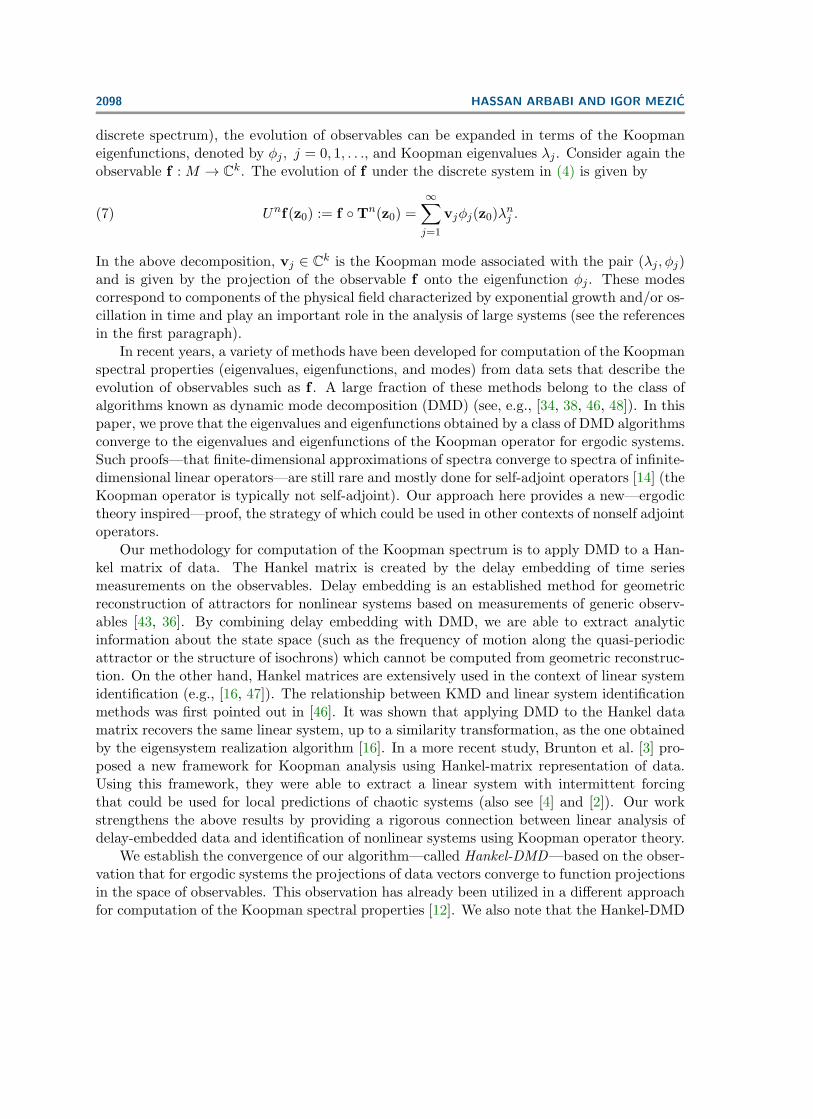
be the matrix of measurements recorded on f along a trajectory starting at the initial conditionz0 ∈ M . Each column of D is called a data snapshot since it contains the measurements onthe system at a single time instant. Assuming only discrete eigenvalues for the Koopmanoperator, we can rewrite the Koopman mode expansion in (7) for each snapshot in the form

Di :=

f1 T i(z0)f2 T i(z0)

...fn T i(z0)

=∞∑j=1

λijvj(10)

by absorbing the scalar values of φj(z0) into the mode vj . In numerical approximation of theKoopman modes, however, we often assume this expansion is finite dimensional and use

f i =n∑j=1

λijvj ,(11)

where vj and λj are approximations to the Koopman modes and eigenvalues in (10). Thisexpansion resembles the spectral expansion for a linear operator acting on Rn. This operator,which maps each column of D to the next is called the DMD operator. The general strategy ofDMD algorithms is to construct the DMD operator, in the form of a matrix, and then extractthe dynamic modes and eigenvalues from the spectrum of that matrix. In the companion-matrix algorithm (Algorithm 1), as the name suggests, the DMD operator is realized in theform of a companion matrix.

Algorithm 1 Companion-matrix DMD.Consider the data matrix D defined in (9).

1: Define X = [D0 D1 . . . Dm−1].2: Form the companion matrix

C =

0 0 . . . 0 c01 0 . . . 0 c10 1 . . . 0 c2...

.... . .

......

0 0 . . . 1 cm−1

(12)

with (c0, c1, c2, . . . , cm−2

)T = X†Dm.

X† denotes the Moore–Penrose pseudoinverse of X [45].3: Let (λj , wj), j = 1, 2, . . . ,m, be the eigenvalue-eigenvector pairs for C. Then the λj ’s are

the dynamic eigenvalues. Dynamic modes vj are given by

vj = Xwj , j = 1, 2, . . . ,m.(13)


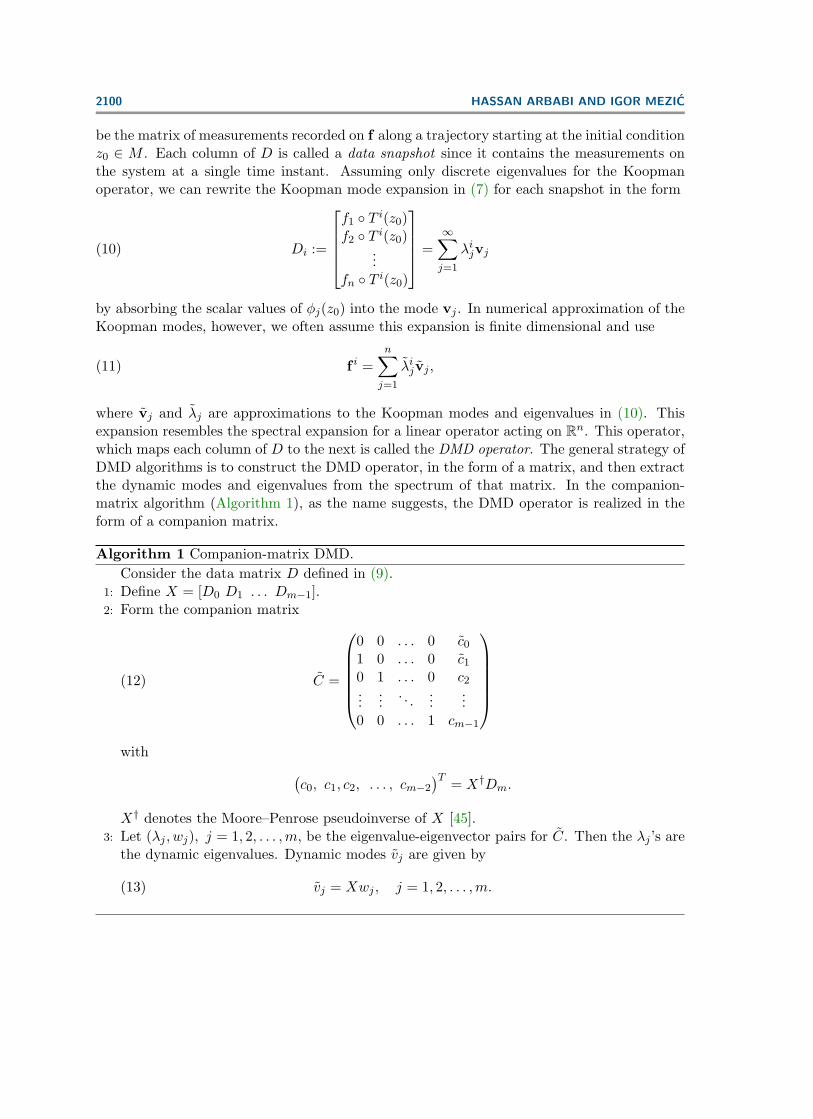
In the above algorithm, the companion matrix C is the realization of the DMD operatorin the basis which consists of the columns in X. The pseudoinverse in step 2 is used to projectthe last snapshot of D onto this basis. In that case that Dm lies in the range of X, we have

r := Dm −X(X†Dm) = 0(14)

which means that the companion matrix C exactly maps each column of D to the next. Ifcolumns of X are linearly dependent, however, the above projection is not unique, and theproblem of determining the DMD operator is generally overconstrained. Furthermore, whenX is ill-conditioned, the projection in step 2 becomes numerically unstable.

The SVD-enhanced DMD algorithm (Algorithm 2), offers a more robust algorithm forcomputation of dynamic modes and eigenvalues.

Algorithm 2 SVD-enhanced DMD.Consider the data matrix D defined in (9).

1: Define X = [D0 D1 . . . Dm−1] and Y = [D1 D2 . . . Dm].2: Compute the SVD of X:

X = WSV ∗.

3: Form the matrix

A = W ∗Y V S−1.

4: Let (λj , wj), j = 1, 2, . . . ,m, be the eigenvalue-eigenvector pairs for A. Then the λj ’s arethe dynamic eigenvalues. Dynamic modes vj are given by

vj = Wwj , j = 1, 2, . . . ,m.

In this method, the left singular vectors W are used as the basis to compute a realizationof the DMD operator, which is A. In fact, column vectors in W form an orthogonal basiswhich enhances the numerical stability of the projection process (the term W ∗Y in step 3).When X is full rank and the λj ’s are distinct, the dynamic modes and eigenvalues computedby this algorithm are the same as the companion-matrix algorithm [7].

The exact DMD algorithm (Algorithm 3) generalizes the SVD-enhanced algorithm to thecase where the sampling of the data might be nonsequential. For example, consider the datamatrices

X =

f1(z0) f1(z1) . . . f1(zm)f2(z0) f2(z1) . . . f2(zm)

......

. . ....

fn(z0) fn(z1) . . . fn(zm)

(15)


and

Y =

f1 T (z0) f1 T (z1) . . . f1 T (zm)f2 T (z0) f2 T (z1) . . . f2 T (zm)

......

. . ....

fn T (z0) fn T (z1) . . . fn T (zm)

,(16)

where z0, z1, . . . , zm denotes a set of arbitrary states of the dynamical system in (4). Theexact DMD algorithm computes the operator that maps each column ofX to the correspondingcolumn in Y .

Algorithm 3 Exact DMD.Consider the data matrices X and Y defined in (15) and (16).

1: Define X = [D0 D1 . . . Dm−1] and Y = [D1 D2 . . . Dm].2: Compute the SVD of X:

X = WSV ∗.

3: Form the matrix

A = W ∗Y V S−1.

4: Let (λj , wj), j = 1, 2, . . . ,m, be the eigenvalue-eigenvector pairs for A. Then the λj ’s arethe dynamic eigenvalues.

5: The exact dynamic modes vj are given by

vj =1λjY V S−1wj , j = 1, 2, . . . ,m.

6: The projected dynamic modes χj are given by

χj = Wwj , j = 1, 2, . . . ,m.

The finite-dimensional operator that maps the columns of X to Y is known as the exactDMD operator with the explicit realization

A = Y X†.(17)

The matrix A is not actually formed in Algorithm 3; however, the dynamic eigenvalues andexact dynamic modes form the eigendecomposition of A. We note that the projected dynamicmodes and exact dynamic modes coincide if the column space of Y lies in the range of X.Moreover, applying exact DMD to X and Y matrices defined in Algorithm 2 yields the sameeigenvalues and modes as SVD-enhanced DMD.

In the following, we will show how DMD operators converge to a finite-dimensional repre-sentation of the Koopman operator for ergodic systems. The critical observation that enablesus to do so is the fact that vector projections in the DMD algorithm can be used to approxi-mate the projections in the function space of observables.


3. Ergodic theory and Hankel-matrix representation of data. In this section, we recallthe elementary ergodic theory and give a new interpretation of Hankel-matrix representationof data in the context of the Koopman operator theory. The main result of this section isProposition 3.1 which asserts the convergence of companion-matrix Hankel-DMD for compu-tation of the Koopman spectrum. Despite the intuitive proof of its convergence, this methodis not well-suited for numerical practice, and a more suitable alternative for numerical com-putation will be presented in sections 5 and 6. In subsection 3.1, we present analogous resultsfor the basin of attraction of ergodic attractors.

Consider the dynamics on a compact invariant set A, possibly the attractor of a dissipativedynamical system, given by the measure-preserving map T : A→ A. Let µ be the preservedmeasure with µ(A) = 1, and assume that for every invariant set B ⊂ A, µ(B) = 0 orµ(A− B) = 0, i.e., the map T is ergodic on A. A few examples of ergodic sets in dynamicalsystems are limit cycles, tori with uniform flow, and chaotic sets like the Lorenz attractor. Wedefine the Hilbert space H to be the set of all observables on A which are square integrablewith respect to the measure µ, i.e.,

(18) H :=f : A→ R s.t.

∫A|f |2dµ <∞

.

The Birkhoff’s ergodic theorem [32] asserts the existence of infinite-time averages of suchobservables and relates it to the spatial average over the set A. More precisely, if f ∈ H, then

limN→∞

1N

N−1∑k=0

f T k(z) =∫Afdµ, for almost every z ∈ A.(19)

An important consequence of this theorem is that the inner products of observables in Hcan be approximated using the time series of observations. To see this, denote by fm(z0)and gm(z0) the vector of m sequential observations made on observables f, g ∈ H along atrajectory starting at z0,

fm(z0) = [f(z0), f T (z0), . . . , f Tm−1(z0)],(20a)

gm(z0) = [g(z0), g T (z0), . . . , g Tm−1(z0)].(20b)

Then for almost every z0 ∈ A,

limm→∞

1m< fm(z0), gm(z0) >= lim

m→∞

1m

m−1∑k=0

(fg∗) T k(z0) =∫Afg∗dµ =< f, g >H,(21)

where we have used < ., . > for the vector inner product and < ., . >H for the inner productof functions in H. The key observation in this work is that using the data vectors such asfm(z0) we can approximate the projection of observables onto each other according to (21).

Now consider the longer sequence of observations

fm+n = [f(z0), f T (z0), . . . , f Tm−1(z0), . . . , f Tm+n−1(z0)]


which could be rearranged into a Hankel matrix by delay embedding of dimension m,

H =

f(z0) f T (z0) . . . f Tn(z0)

f T (z0) f T 2(z0) . . . f Tn+1(z0)...

.... . .

...f Tm−1(z0) f Tm(z0) . . . f Tm+n−1(z0)

.(22)

Given the definition of the Koopman operator in (5), we also observe that the jth column ofthis matrix is the sampling of the observable U j−1f along the same trajectory, and we canrewrite it in a more compact form,

H =(fm, U fm, . . . , U

nfm

).

This matrix can be viewed as a sampling of the Krylov sequence of observable f , defined as

Fn := [f, Uf, . . . , Unf ].

The basic idea of the Hankel-DMD method is to extract the Koopman spectra from thissequence, which is analogous to the idea of Krylov subspace methods for computing theeigenvalues of large matrices [35]. A simplifying assumption that we utilize in most of thispaper is that there exists a finite-dimensional subspace of H which is invariant under theaction of the Koopman operator and contains our observable of interest f . In general, theexistence of finite-dimensional Koopman-invariant subspaces is equivalent to the existence ofthe eigenvalues (i.e., discrete spectrum) for the Koopman operator. To be more precise, ifsuch an invariant subspace exists, then the Koopman operator restricted to this subspace canbe realized in the form of a finite-dimensional matrix and therefore it must have at least one(complex) eigenvalue. Conversely, if the Koopman operator has eigenvalues, the span of afinite number of associated eigenfunctions forms an invariant subspace. However, it is notguaranteed that the arbitrary observables such as f are contained within such subspaces.

Let k be the dimension of the minimal Koopman-invariant subspace, denoted by K, whichcontains f . Then the first k iterates of f under the action of the Koopman operator span K,i.e.,

(23) K = span(Fn) for every n ≥ k − 1.

This condition follows from the fact that the Koopman eigenvalues are simple for ergodicsystems [13] and, as a result, f is cyclic in K [24]. The following proposition shows thatthe eigenvalues and eigenfunctions obtained by applying DMD to H converge to true eigen-functions and eigenvalues of the Koopman operator. Our proof strategy is to show that thecompanion matrix formed in Algorithm 1 approximates the k-by-k matrix which representsthe Koopman operator restricted to K.

Proposition 3.1 (convergence of the companion-matrix Hankel-DMD algorithm). Let thedynamical system in (4) be ergodic, and Fn = [f, Uf, . . . , Unf ] span a k-dimensional subspaceof H (with k < n) which is invariant under the action of the Koopman operator. Consider the


dynamic eigenvalues and dynamic modes obtained by applying the companion-matrix DMD(Algorithm 1) to the first k + 1 columns of the Hankel matrix Hm×n defined in (22).

Then, for almost every z0, as m→∞,(a) the dynamic eigenvalues converge to the Koopman eigenvalues associated with the k-

dimensional subspace;(b) the dynamic modes converge to the sampling of associated Koopman eigenfunctions on

the trajectory starting at z0.

Proof. Consider the first k elements of Fn,(f, Uf, . . . , Uk−1f

)(24)

which are linearly independent. These observables provide a basis for K, and the restrictionof the Koopman operator to K can be (exactly) realized as the companion matrix

C =

0 0 . . . 0 c01 0 . . . 0 c10 1 . . . 0 c2...

.... . .

......

0 0 . . . 1 ck−1

,

where the last column is the coordinate vector of the function Ukf in the basis, and it is givenby

c0c1...

ck−1

= G−1

< f,Ukf >H< Uf,Ukf >H

...< Uk−1f, Ukf >H

.(25)

Here, G is the Gramian matrix of the basis given by

Gij =< U i−1f, U j−1f >H .

Now consider the numerical companion-matrix DMD algorithm and let X be the matrix thatcontains the first k columns of H. When applied to the first k+1 columns of H, the algorithmseeks the eigenvalues of the companion matrix C, whose last column is given by

c0c1...

ck−1

= X†Ukfm = G−1

1m < fm, U

kfm >1m < Ufm, U

kfm >...

1m < Uk−1fm, U

kfm >

.(26)

In the second equality, we have used the following relationship for the Moore–Penrose pseudo-inverse of a full-rank data matrix X,

X† = (X∗X)−1X∗ =(

1mX∗X

)−1( 1mX∗)

:= G−1(

1mX∗)


and defined the numerical Gramian matrix by

Gij =1m< U i−1fm, U

j−1fm > .

The averaged inner products in the rightmost vector of (26) converge to the vector ofHilbert-space inner products in (25), due to (21). The same argument suggests elementwiseconvergence of the numerical Gramian matrix to the G in (25), i.e.,

limm→∞

Gij = Gij .

Furthermore

limm→∞

G−1 =(

limm→∞

G)−1

= G−1.

We have interchanged the limit and inverting operations in the above since G is invertible(because the basis is linearly independent). Thus the DMD operator C converges to theKoopman operator realization C. The eigenvalues of matrix depend continuously on its entrieswhich guarantees the convergence of the eigenvalues of C to the eigenvalues of C as well. Thisproves the statement in (a). Now let vk be the set of normalized eigenvectors of C, that is,

Cvj = λjvj , ‖vj‖ = 1, j = 1, . . . , k.

These eigenvectors give the coordinates of Koopman eigenfunctions in the basis of (24).Namely, φj , j = 1, . . . , k, defined by

φi =(f, Uf, . . . , Uk−1f

)vi, i = 1, . . . , k,(27)

are a set of Koopman eigenfunctions in the invariant subspace. Given the convergence ofC to C and convergence of their eigenvalues, the normalized eigenvectors of C, denoted byvj , j = 0, 1, . . . , k, also converge to the vj ’s. We define the set of candidate functions by

φi =(f, Uf, . . . , Uk−1f

)vi, i = 1, . . . , k,(28)

and show that they converge to φi as m→∞. Consider an adjoint basis of (24) denoted bygj, j = 0, 1, . . . , k − 1, defined such that < gi, U

jf >H= δij with δ being the Kroneckerdelta. We have

limm→∞

< φi, gj >H= limm→∞

vij = vij =< φi, gj >H,

where vij is the ith entry of vj . The above statement shows the weak convergence of the φjto φj for j = 1, . . . , k. However, both set of functions belong to the same finite-dimensionalsubspace and therefore weak convergence is strong convergence. The jth dynamic mode givenby

wi =(fm, U fm, . . . , U

k−1fm

)vi(29)

is the sampling of φj along the trajectory, and convergence of φj means that wj converges tothe value of Koopman eigenfunction φj on the trajectory starting at z0. The proposition isvalid for almost every initial condition for which the ergodic average in (19) exists.


Remark 1. In the above results, the data vectors can be replaced with any sampling vectorof the observables that satisfy the convergence of inner products as in (21). For example,instead of using f as defined in (20a), we can use the sampling vectors of the form

fm(z0) = [f(z0), f T l(z0), f T 2l(z0), . . . , f T (m−1)l(z0)],

where l is a positive finite integer.

3.1. Extension of Hankel-DMD to the basin of attraction. Consider the ergodic set Ato be an attractor of the dynamical system (4) with a basin of attraction B. The existenceof ergodic averages in (19) can be extended to trajectories starting in B by assuming that theinvariant measure on A is a physical measure [9, 49]. To formalize this notion, let ν denotethe standard Lebesgue measure on B. We assume that there is a subset B ⊂ B such thatν(B−B) = 0 and for every initial condition in B the ergodic averages of continuous functionsexist. That is, if f : B → R is continuous, then

limN→∞

1N

N∑k=0

f T k(z) =∫Afdµ for ν-almost every z ∈ B.(30)

Roughly speaking, this assumption implies that the invariant measure µ rules the asymptoticsof almost every trajectory in B, and therefore it is relevant for physical observations andexperiments. Using (30), we can extend Proposition 3.1 to the trajectories starting almosteverywhere in B. The only extra requirement is that the observable must be continuous in thebasin of attraction.

Proposition 3.2 (convergence of Hankel-DMD inside the basin of attraction). Let A be theergodic attractor of the dynamical system (4) with the basin of attraction B which supportsa physical measure. Assume f : B → R is a continuous function with f |A belonging toa k-dimensional Koopman-invariant subspace of H. Let H be the Hankel matrix (22) ofobservations on f along the trajectory starting at z0 ∈ B with n > k. Consider the dynamicmodes and eigenvalues obtained by applying the companion-matrix DMD (Algorithm 1) to thefirst k + 1 columns of H.

Then, for ν-almost every z0, as m→∞,(a) the dynamic eigenvalues converge to the Koopman eigenvalues;(b) the dynamic modes converge to the value of associated eigenfunctions φj along the

trajectory starting at z0.

Proof. The proof of (a) is similar to Proposition 3.1 and follows from the extension ofergodic averages to the basin of attraction by (30). To show that the dynamic mode wjconverges to Koopman eigenfunctions along the trajectory, we need to consider the evolution


of wj under the action of the Koopman operator:

limm→∞

Uwj = limm→∞

U [fm, Ufm, . . . , Uk−1fm]vj

= limm→∞

[Ufm, U2fm, . . . , Ukfm]vj

= limm→∞

[fm, Ufm, . . . , Uk−1fm]Cvj

= limm→∞

[Ufm, U2fm, . . . , Ukfm]λj vj

= limm→∞

λjwj

= λjwj .

Therefore, wj converges to the sampling of values of the eigenfunction associated with eigen-value λj .

4. SVD and POD for ergodic systems. SVD is a central algorithm of linear algebrathat lies at the heart of many data analysis techniques for dynamical systems including linearsubspace identification methods [47] and DMD [38, 46]. POD, on the other hand, is a dataanalysis technique frequently used for complex and high-dimensional dynamical systems. Alsoknown as principal component analysis, or Karhonen–Loeve decomposition, POD yields anorthogonal basis for representing an ensemble of observations which is optimal with respectto a predefined inner product. It is known that for finite-dimensional observables on discrete-time dynamical systems, POD reduces to SVD [15]. Here, we establish a slightly differentconnection between these two concepts in the case of ergodic systems. Our motivation forderivation of these results is the role of SVD in DMD algorithms; however, the orthogonalbasis that is generated by this process can be used for further analysis of dynamics in thespace of observables, for example, to construct a basis for computing the eigenfunctions ofthe Koopman generator as in [12]. We first review POD and then record our main result inProposition 4.1.

Let F = [f1, f2, . . . , fn] be an ensemble of observables in the Hilbert space H whichspans a k-dimensional subspace. Applying POD to F yields the expansion

F = ΨΣV ∗(31)

= [ψ1, ψ2, . . . , ψk]

σ1 0 . . . 00 σ2 . . . 0...

.... . .

...0 0 . . . σk

v∗1v∗2...v∗k

,

where the ψj ’s, j = 1, 2, . . . , k, form an orthonormal basis for spanF, and are often calledthe empirical orthogonal functions or POD basis of F . The diagonal elements of Σ, denotedby σj , j = 1, 2, . . . , k, are all positive and signify the H-norm contribution of the basis elementψj to the F . The columns of V , denoted by vi and called the principal coordinates, are thenormalized coordinates of vectors in F with respect to the POD basis. This decomposition


can be alternatively written as a summation,

fi =k∑j=1

σjψjvji.(32)

If we index the principal coordinates such that σ1 > σ2 > · · · > σk > 0, then this decomposi-tion minimizes the expression

ep =1n

n∑i=1

∥∥∥∥∥∥p∑j=1

σjψjvji − fi

∥∥∥∥∥∥H

for any p ≤ k over the choice of all orthonormal bases for spanF. The term ep denotesthe average error in approximating the fi’s by truncating the sum in (32) at length p. Thisproperty, by design, guarantees that low-dimensional representations of F using truncationsof POD involves the least ‖ · ‖H-error compared to other choices of orthogonal decomposition.

An established method for computation of POD is the method of snapshots [40]: we firstform the Gramian matrix G, given by Gij =< fi, fj >H. The columns of V are given asthe normalized eigenvectors of G associated with its nonzero eigenvalues, and those nonzeroeigenvalues happen to be σ2

i ’s, that is,

GV = V Σ2.(33)

Since G is a symmetric real matrix, V will be an orthonormal matrix and the decompositionin (31) can be easily inverted to yield the orthonormal basis functions,

ψj =1σjFvj .

The SVD of a tall rectangular matrix has a similar structure to POD. Consider Xm×n, withm > n, to be a matrix of rank r. The reduced SVD of X is

X = WSV ∗(34)

=

w1 w2 . . . wr

s1 0 . . . 00 s2 . . . 0...

.... . .

...0 0 . . . sr

v∗1v∗2...v∗r

,where W and V are orthonormal matrices, and S is a diagonal matrix holding the singularvalues s1 > s2 > · · · > sr > 0. The columns of W and V are called, respectively, left andright singular vectors of X.

The usual practice of POD in data analysis is to let H be the space of snapshots, e.g., Rm

equipped with the usual Euclidean inner product, which makes POD and SVD identical [15].In that case, F would be a snapshot matrix such as (9) and its left singular vectors are thePOD basis. We are interested in H, however, as the infinite-dimensional space of observables


defined in (18). Given the sampling of a set of observables on a single ergodic trajectory, ourcomputational goal is to get the sampling of the orthonormal basis functions for the subspaceof H spanned by those observables. The next proposition shows that this can be achieved byapplying SVD to a data matrix whose columns are ergodic samplings of those observables.Incidentally, such a matrix is the transpose of a snapshot matrix!

Proposition 4.1 (convergence of SVD to POD for ergodic systems). Let F = [f1, f2, . . . , fn]be an ensemble of observables on the ergodic dynamical system in (4). Assume F spans a k-dimensional subspace of H and let

F = ΨΣV ∗

be the POD of F . Now consider the data matrix

F =

f1(z0) f2(z0) . . . fn(z0)

f1 T (z0) f2 T (z0) . . . fn T (z0)...

.... . .

...f1 Tm−1(z0) f2 Tm−1(z0) . . . fn T (z0)

(35)

and let

1√mF ≈WSV ∗

be the reduced SVD of (1/√m)F .

Then, for almost every z0, as m→∞,(a) sj → σj for j = 1, 2, . . . , k and sj → 0 for j = k + 1, . . . , n;(b) vj → vj for j = 1, 2, . . . , k;(c)√mwj converges to the sampling of ψj along the trajectory starting at z0 j = 1, 2, . . . , k.

Proof. Consider the numerical Gramian matrix

G :=(

1√mF

)∗( 1√mF

)=

1mF ∗F .

As shown in the proof of Proposition 3.1, the assumption of ergodicity implies the convergenceof G to the Gramian matrix G in (33) as m → ∞. Now denote by λj , j = 1, 2, . . . , k, the keigenvalues of G that converge to positive eigenvalues of G, and denote by λ′j , j = 1, . . . , n−k,the eigenvalues of G that converge to zero. There exists m0 such that for any m > m0, all thesingular values sj =

√λj are larger than s′j =

√λ′j and therefore occupy the first k diagonal

entries of S, which completes the proof of statement in (a).The statement in (b) follows from the convergence of the normalized eigenvectors of G

associated with λj ’s to those of G. To show that (c) is true, we first construct the candidatefunctions by letting

ψj =1sjF vj , j = 1, 2, . . . , k.(36)


We compute the entries of the orthogonal projection matrix P defined by Pi,j =< ψi, ψj >and consider its limit as m→∞:

limm→∞

Pi,j = limm→∞

(1σiFvi

)∗( 1sjF vj

)=

1σiv∗iF∗F lim

m→∞

1sjvj =

1σ2i

v∗iGvj = δij .(37)

In the last equality, we have used (33). This calculation shows that the ψj ’s are weaklyconvergent to the ψj ’s, and since they belong to the same finite-dimensional space, thatimplies strong convergence as well. Noting the definition of left singular vector

wj =1√msj

F vj ,(38)

it is easy to see that√mwj is the sampling of the candidate function ψj along the trajectory

starting at z0.

4.1. Representation of chaotic dynamics in the space of observables using the Hankelmatrix and SVD. Using the above results, we are able to construct an orthonormal basison the state space from the time series of an ergodic system and give a new data-drivenrepresentation of chaotic dynamical systems. Recall that the columns of the Hankel matrixH defined in (22) provide an ergodic sampling of the Krylov sequence of observables Fn =[f, Uf, , Unf ] along a trajectory in the state space. Therefore by applying SVD to H, we canapproximate an orthonormal basis for Fn and, furthermore, represent the Koopman evolutionof observable f in the form of principal coordinates.

We show an example of this approach using the well-known chaotic attractor of the Lorenzsystem [22]. This attractor is proven to have the mixing property which implies ergodicity[23]. The Lorenz system is given by

z1 = σ(z2 − z1),z2 = z1(ρ− z3)− z2,

z3 = z1z2 − βz3,

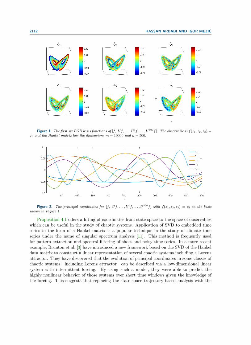
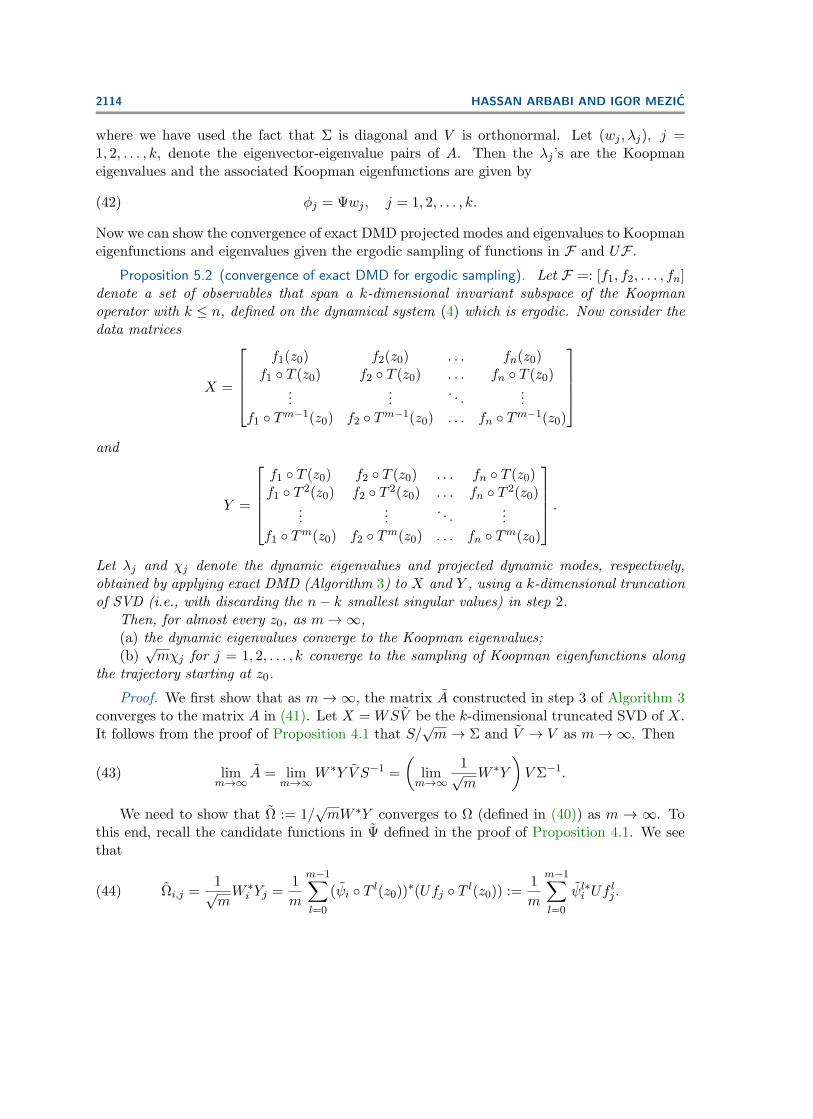
with [z1, z2, z3] ∈ R3 and parameter values σ = 10, ρ = 28, and β = 8/3. First, we samplethe value of observable f(z) = z1 every 0.01 seconds on a random trajectory, and then forma tall Hankel matrix as in (22) with m = 10000 and n = 500. Figure 1 shows the values ofthe first six left singular vectors of the Hankel matrix, which approximate the basis functionsψj . The corresponding right singular vectors, shown in Figure 2, approximate the principalcoordinates of Fn. We make note that the computed basis functions and their associatedsingular values show little change with m for m ≥ 10000.

In mixing attractors such as Lorenz, the only discrete eigenvalue for the Koopman operatoris λ = 0, which is associated with an eigenfunction that is constant almost everywhere on theattractor. In this case, the Koopman operator cannot have any invariant finite-dimensionalsubspace other than the span of almost-everywhere constant functions. As a result, for atypical observable f , the Krylov sequence Fn is always (n+ 1)-dimensional and growing withiterations of U . This observation shows that despite the fact that evolution of principal co-ordinates in Figure 2 is linear, there is no finite-dimensional linear system that can describetheir evolution.


Figure 1. The first six POD basis functions of [f, Uf, . . . , U if, . . . , U500f ]. The observable is f(z1, z2, z3) =z1 and the Hankel matrix has the dimensions m = 10000 and n = 500.

Figure 2. The principal coordinates for [f, Uf, . . . , U if, . . . , U500f ] with f(z1, z2, z3) = z1 in the basisshown in Figure 1.

Proposition 4.1 offers a lifting of coordinates from state space to the space of observableswhich can be useful in the study of chaotic systems. Application of SVD to embedded timeseries in the form of a Hankel matrix is a popular technique in the study of climate timeseries under the name of singular spectrum analysis [11]. This method is frequently usedfor pattern extraction and spectral filtering of short and noisy time series. In a more recentexample, Brunton et al. [3] have introduced a new framework based on the SVD of the Hankeldata matrix to construct a linear representation of several chaotic systems including a Lorenzattractor. They have discovered that the evolution of principal coordinates in some classes ofchaotic systems—including Lorenz attractor—can be described via a low-dimensional linearsystem with intermittent forcing. By using such a model, they were able to predict thehighly nonlinear behavior of those systems over short time windows given the knowledge ofthe forcing. This suggests that replacing the state-space trajectory-based analysis with the


evolution of coordinates in the space of observables gives a more robust representation of thedynamics for analysis and control purposes.

5. Convergence of exact DMD and extension to multiple observables. In this section,we review the functional setting for exact DMD and prove its convergence for ergodic systemsusing the assumption of invariant subspace. We then discuss using this method combined withHankel matrices to compute the Koopman spectra from observations on single or multipleobservables. The summary of the numerical algorithm with several examples will be given inthe next section.

Let F =: [f1, f2, . . . , fn] denote a set of observables defined on the discrete dynamicalsystem in (4). We make the assumption that F spans a k-dimensional subspace of H with k ≤n, which is invariant under the Koopman operator. Also denote by UF =: [Uf1, Uf2, . . . , Ufn]the image set of those observables under the action of the Koopman operator. We seek torealize the Koopman operator, restricted to this subspace, as a k-by-k matrix, given theknowledge of F and UF .

Let

F = ΨΣV ∗(39)

be the POD of ensemble F with Ψ = [ψ1, ψ2, . . . , ψk] denoting its POD basis. Since Fspans an invariant subspace, the functions in UF also belong to the same subspace and theirprincipal coordinates can be obtained by orthonormal projection, i.e.,

Ω = Ψ∗UF .(40)

The restriction of the Koopman operator to the invariant subspace is then given by matrix Awhich maps the columns of ΣV ∗ to the columns of Ω. The following lemma, which summarizessome of the results in [46], gives the explicit form of matrix A and asserts its uniqueness underthe prescribed condition on F and UF .

Lemma 5.1. Let Xk×n with n ≥ k be a matrix whose range is equal to Rk. Let Yk×n beanother matrix which is linearly consistent with X, i.e., whenever Xc = 0 for c ∈ Rn, thenY c = 0 as well. Then the exact DMD operator A := Y X† is the unique matrix that satisfiesAX = Y .

Proof. First, we note that the condition of Y being linearly consistent with X impliesthat A satisfies AX = Y (Theorem 2 in [46]). To see the uniqueness, let A be another matrixwhich satisfies AX = Y . Now let b ∈ Rk be an arbitrary vector. Given that X spans Rk, wecan write b = Xd for some d ∈ Rn. Consequently,

Ab = AXd = Y d = AXd = Ab,

which means that action of A and A on all elements of Rk is the same, therefore, A = A.

Since F and UF are related through a linear operator, their principal coordinates with respectto the same orthogonal basis satisfy the condition of linear consistency, and the Koopmanoperator restricted to the invariant subspace is represented by the matrix

A = Ω(ΣV ∗)† = ΩV Σ−1,(41)


where we have used the fact that Σ is diagonal and V is orthonormal. Let (wj , λj), j =1, 2, . . . , k, denote the eigenvector-eigenvalue pairs of A. Then the λj ’s are the Koopmaneigenvalues and the associated Koopman eigenfunctions are given by

φj = Ψwj , j = 1, 2, . . . , k.(42)

Now we can show the convergence of exact DMD projected modes and eigenvalues to Koopmaneigenfunctions and eigenvalues given the ergodic sampling of functions in F and UF .

Proposition 5.2 (convergence of exact DMD for ergodic sampling). Let F =: [f1, f2, . . . , fn]denote a set of observables that span a k-dimensional invariant subspace of the Koopmanoperator with k ≤ n, defined on the dynamical system (4) which is ergodic. Now consider thedata matrices

X =

f1(z0) f2(z0) . . . fn(z0)

f1 T (z0) f2 T (z0) . . . fn T (z0)...

.... . .

...f1 Tm−1(z0) f2 Tm−1(z0) . . . fn Tm−1(z0)

and

Y =

f1 T (z0) f2 T (z0) . . . fn T (z0)f1 T 2(z0) f2 T 2(z0) . . . fn T 2(z0)

......

. . ....

f1 Tm(z0) f2 Tm(z0) . . . fn Tm(z0)

.Let λj and χj denote the dynamic eigenvalues and projected dynamic modes, respectively,obtained by applying exact DMD (Algorithm 3) to X and Y , using a k-dimensional truncationof SVD (i.e., with discarding the n− k smallest singular values) in step 2.

Then, for almost every z0, as m→∞,(a) the dynamic eigenvalues converge to the Koopman eigenvalues;(b)√mχj for j = 1, 2, . . . , k converge to the sampling of Koopman eigenfunctions along

the trajectory starting at z0.

Proof. We first show that as m→∞, the matrix A constructed in step 3 of Algorithm 3converges to the matrix A in (41). Let X = WSV be the k-dimensional truncated SVD of X.It follows from the proof of Proposition 4.1 that S/

√m→ Σ and V → V as m→∞. Then

limm→∞

A = limm→∞

W ∗Y V S−1 =(

limm→∞

1√mW ∗Y

)V Σ−1.(43)

We need to show that Ω := 1/√mW ∗Y converges to Ω (defined in (40)) as m → ∞. To

this end, recall the candidate functions in Ψ defined in the proof of Proposition 4.1. We seethat

Ωi,j =1√mW ∗i Yj =

1m

m−1∑l=0

(ψi T l(z0))∗(Ufj T l(z0)) :=1m

m−1∑l=0

ψl∗i Uflj .(44)


Since the ψi’s are defined by a linear combination of functions in F , they lie in the span of Ψ.In fact, we have

ψi =k∑q=1

Pi,qψq,(45)

where Pi,q denotes an entry of the orthogonal projection matrix P defined in the proof ofProposition 4.1. The computation in (37) shows that as m → ∞, we have Pi,q → 0 if q 6= iand Pi,i → 1. Now we replace ψi in (44) with its expansion in (45), while considering the term

d1 : = Ωi,j −1m

m−1∑l=0

(ψi T l(z0))∗(Ufj T l(z0)),(46)

:= Ωi,j −1m

m−1∑l=0

ψl∗i Uflj ,

=k∑q=1

Pi,q1m

m−1∑l=0

ψl∗q Uflj −

1m

m−1∑l=0

ψl∗i Uflj ,

=k∑

q=1, q 6=iPi,q

1m

m−1∑l=0

ψl∗q Uflj + (Pi,i − 1)

1m

m−1∑l=0

ψl∗i Uflj .

The convergence of sums over l for m→∞ in the last line is given by (21). Combining thatwith the convergence of the Pi,q’s, we can conclude that for every ε > 0, there exists m1 suchthat for any m > m1, we have |d1| < ε/2. Now consider the term

d2 =1m

m−1∑l=0

ψl∗i Uflj − Ωi,j(47)

=1m

m−1∑l=0

ψl∗i Uflj− < ψi, Ufj > .

The convergence in (21) again implies that for every ε > 0 there exists an m2 such that forany m > m2, we have |d2| < ε/2. Now it becomes clear that

|Ωi,j − Ωi,j | = |d1 + d2| ≤ |d1|+ |d2| = ε(48)

for any m > max(m1,m2). This proves the convergence of Ω to Ω, which, by revisiting (43),means

limm→∞

A = A.(49)

The eigenvalues of A converge to the eigenvalues of A which are the Koopman eigenvalues.Let wj , j = 1, 2, . . . , k denote the normalized eigenvectors of A, and define the candidate


functions φj = Ψwj = ΨPwj . Given that P converges to I, and wj converges to wj asm→∞, it follows that φj strongly converges to the Koopman eigenfunctions φj = Ψwj .

Now note that√mχj =

√mUwj is the sampling of candidate eigenfunction φj along the

trajectory, and therefore it converges to the sampling of the Koopman eigenfunction φj asm→∞.

Recall that in subsection 3.1, we extended the application of companion-matrix Hankel-DMD to the basin of attraction of an ergodic set A by assuming the invariant measure on Ais physical. An analogous extension of the above proposition can be stated using the sameassumption.

Corollary 5.3. Proposition 5.2 is also valid for ν-almost every z0 ∈ B (ν is the Lebesguemeasure), where B is the basin of attraction for the ergodic attractor A of the dynamical system(4), given that

(i) the invariant measure on A is a physical measure;(ii) F|A spans a k-dimensional invariant subspace of H; and(iii) F is continuous over B.

Proof. The proof is similar to Proposition 3.2.

Let us first consider the application of the above proposition using measurements on asingle observable f . We can supplement those measurements using delay embedding whichis equivalent to setting F = [f, Uf, . . . , Un−1f ]. An ergodic sampling of F and UF is thengiven by data matrices

X = H, Y = UH,

where H is the Hankel matrix defined in (22) and UH is the same matrix but shifted onestep forward in time. In such a case, the exact DMD reduces to the SVD-enhanced DMD asdiscussed in section 2.

In the case of multiple observables, we can combine the delay-embedded measurements ofthe observables with each other. For example, let f and g be the only observables that couldbe measured on a dynamical system. Then, we let F1 = [f, Uf, . . . , U l−1f, g, Ug, . . . , U q−1g]and data matrices would contain blocks of Hankel matrices, i.e.,

X =[Hf Hg

], Y =

[UHf UHg

].(50)

The above proposition guarantees the convergence of the exact DMD method if l and q arechosen large enough, e.g., l, q > k + 1, where k is the dimension of the invariant subspacecontaining f and g.

In numerical practice, however, the block Hankel matrices need some scaling. For instanceassume ‖g‖H ‖f‖H. The POD basis that corresponds to the measurements on g is asso-ciated with smaller singular values and might be discarded through a low-dimensional SVD


truncation. To remedy this issue, we can use the fact that the ratio of the norm betweenobservables in ergodic systems can be approximated from the measurements:

α :=‖f‖H‖g‖H

= limm→∞

‖fm‖‖gm‖

,(51)

where fm and gm are the observation vectors defined in (20a). The scaled data matrices inthat case become

X =[Hf αHg

], Y =

[UHf αUHg

].(52)

6. Numerical application of Hankel-DMD method. Algorithm 4 summarizes the Hankel-DMD method for extracting the Koopman spectrum from single or multiple observables. Thisalgorithm acts on Hankel matrices of the data in the form of

H i =

fi(zi) fi T (zi) . . . fi Tn(zi)

fi T (zi) fi T 2(zi) . . . fi Tn+1(zi)...

.... . .

...fi Tm−1(zi) fi Tm(zi) . . . fi Tm+n−1(zi)

, i = 1, 2, . . . l,(53)

and UH i which is the same matrix shifted forward in time. The data on observable fi iscollected from a trajectory starting at zi which is in the basin of attraction of an ergodicattractor. Unlike the classical DMD algorithms in section 2, the number of modes obtainedby this method depends on the length of the signal and the dimension of subspace in whichthe observable lies.

The rate of convergence for the Hankel-DMD can be established by considering the rateof convergence for ergodic averages. For periodic and quasi-periodic attractors, the error ofapproximating the inner products by (21) is generally bounded by |c/m| for some c ∈ R [31].For strongly mixing systems, the rate of convergence slows down to c/

√m. However, for the

general class of ergodic systems convergence rates cannot be established [20]. As we will see inthis section, a few hundred samples would be enough to determine the Koopman frequenciesof periodic systems with great accuracy, while a few thousand would be enough for systemswith a 2-torus attractor.

Remark 2. In proving the convergence of the Hankel-DMD algorithm, we have assumedthe explicit knowledge of the dimension of the invariant subspace (k) that contains the observ-able. In numerical practice, k can be found in the SVD step of the algorithm: Proposition 4.1showed that as m→∞, the number of singular values converging to positive values is equal tok. Therefore, we can approximate the invariant subspace by counting the number of singularvalues that don’t seem to decay to zero. We can implement this assumption in Algorithm 4by hard thresholding of the SVD in step 3, i.e., discarding the singular values that are smallerthan a specified threshold. Such a threshold can be selected based on the desired numericalaccuracy and considering the rate of convergence for ergodic averages which is discussed above.In the case that the observable lies in an infinite-dimensional Koopman invariant subspace, weare going to assume that it lives in a finite-dimensional subspace down to a specific numericalaccuracy. We can enforce this accuracy, again, by hard thresholding the SVD. In the followingexamples, we have chosen the hard threshold of SVD to be 1e-10.


Algorithm 4 Hankel DMD.Consider the Hankel matrices H i’s defined in (53).

1: Compute the scaling factors

αi =‖H i

n+1‖‖H1

n+1‖, i = 2, 3, . . . , l,

where H in+1 is the last column of H i.

2: Form the composite matrices

X =[H1 α2H2 . . . αlHl

], Y =

[UHf α2UH2 . . . αlUHl

].

3: Compute the truncated SVD of X (see Remark 2):

X = WSV ∗.

4: Form the matrix

A = W ∗Y V S−1.

5: Let (λj , wj), j = 1, 2, . . . ,m, be the eigenvalue-eigenvector pairs for A. Then the λj ’sapproximate the Koopman eigenvalues.

6: The dynamic modes χj given by

χj = Wwj , j = 1, 2, . . . ,m,

approximate the Koopman eigenfunctions.

6.1. Application to single observable: Periodic and quasi-periodic cavity flow. In aprevious study by the authors [1], the lid-driven cavity flow was shown to exhibit periodic andquasi-periodic behavior at Reynolds numbers (Re) in the range of 10000–18000. The Koop-man eigenvalues were computed by applying an adaptive combination of FFT and harmonicaveraging to the discretized field of the stream function, which is an observable with ∼ 4000values. We use the Hankel-DMD method (Algorithm 4) to extract the Koopman eigenval-ues and eigenfunctions using a scalar-valued observable (the kinetic energy) and compare ourresults with the following cases studied in [1]:

• At Re = 13000, the trajectory in the state space of the flow converges to a limitcycle with the basic frequency of ω0 = 1.0042 rad/sec. The Koopman frequencies inthe decomposition of analytic observables are multiples of the basic frequency, i.e.,kω0, k = 0, 1, 2, . . ..• At Re = 16000, the posttransient flow is quasi-periodic with two basic frequenciesω1 = 0.9762 rad/sec and ω2 = 0.6089 rad/sec. In this case, the flow trajectory wrapsaround a 2-torus in the state space of the flow and the Koopman frequencies areintegral multiples of ω1 and ω2, that is ω = k · (ω1, ω2), k ∈ Z2.


Table 1The dominant Koopman frequencies and eigenfunctions for periodic cavity flow computed using observations

on kinetic energy.

k ωk ωk ([1]) Relative error var(φk − φk)0 0 0 0 < 1e−101 1.00421 1.00423 1.59e−5 1.46e−62 2.00843 2.00840 1.56e−5 2.25e−53 3.01264 3.01262 4.94e−6 < 1.00e−104 4.01685 4.01680 1.55e−5 < 1.00e−106 6.02528 6.02525 5.03e−6 < 1.00e−10

Let Ei := E(t0 + i∆t) denote the measurements on the kinetic energy of the flow atthe time instants t0 + i∆t, i = 0, 1, 2, . . . , s. We first build the Hankel matrices of the kineticenergy observable,

HE =

E0 E1 . . . EnE1 E2 . . . En+1E2 E3 . . . En+2...

.... . .

...Em−1 Em . . . Em+n−1

, UHE =

E1 E2 . . . En+1E2 E3 . . . En+2E3 E4 . . . En+3...

.... . .

...Em Em+1 . . . Em+n

,(54)

and then apply Algorithm 4. Due to the discrete-time nature of the measurements, theeigenvalues computed by this method correspond to the discrete map obtained by strobingthe original continuous-time dynamical system at intervals of length ∆t. The eigenvaluesλj , j = 1, 2, . . . , computed via Hankel DMD are related to the Koopman frequencies ωj , j =1, 2, . . . through the following:

λj = eiωj∆t.

The computed dynamic modes φj approximate the value of the associated Koopman eigen-functions along the first m points on the trajectory of the system.

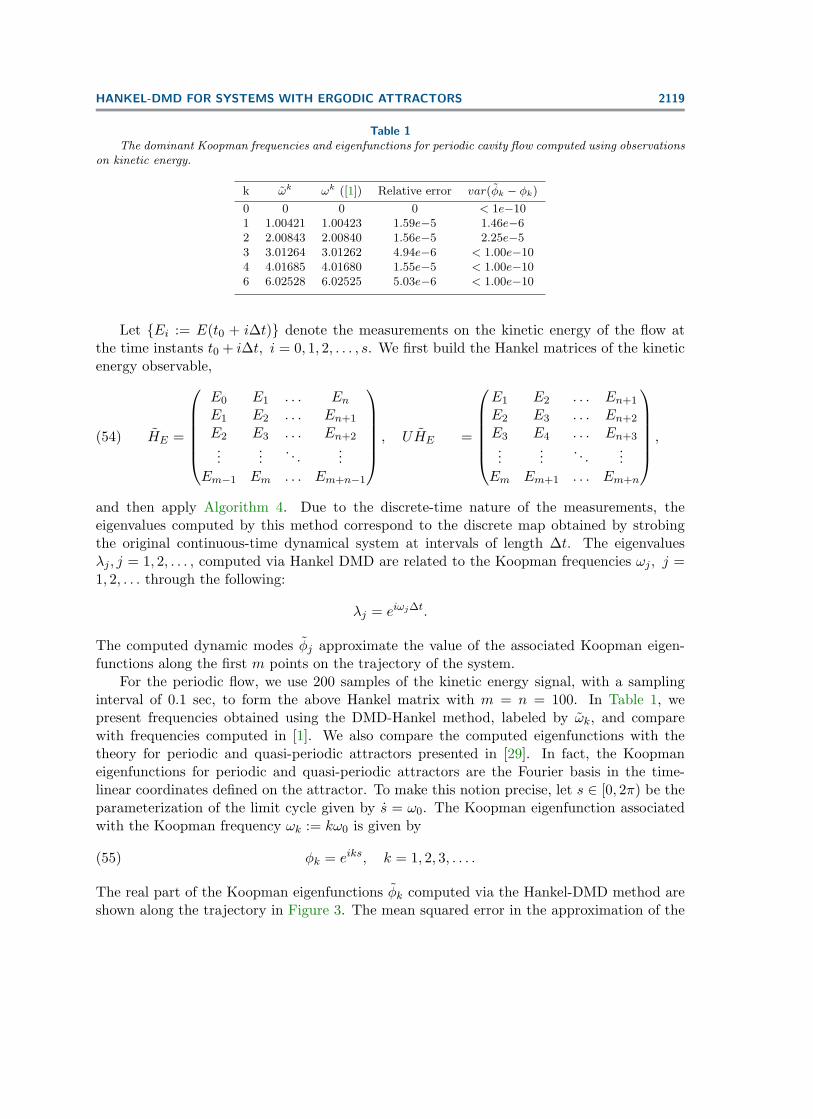
For the periodic flow, we use 200 samples of the kinetic energy signal, with a samplinginterval of 0.1 sec, to form the above Hankel matrix with m = n = 100. In Table 1, wepresent frequencies obtained using the DMD-Hankel method, labeled by ωk, and comparewith frequencies computed in [1]. We also compare the computed eigenfunctions with thetheory for periodic and quasi-periodic attractors presented in [29]. In fact, the Koopmaneigenfunctions for periodic and quasi-periodic attractors are the Fourier basis in the time-linear coordinates defined on the attractor. To make this notion precise, let s ∈ [0, 2π) be theparameterization of the limit cycle given by s = ω0. The Koopman eigenfunction associatedwith the Koopman frequency ωk := kω0 is given by

φk = eiks, k = 1, 2, 3, . . . .(55)

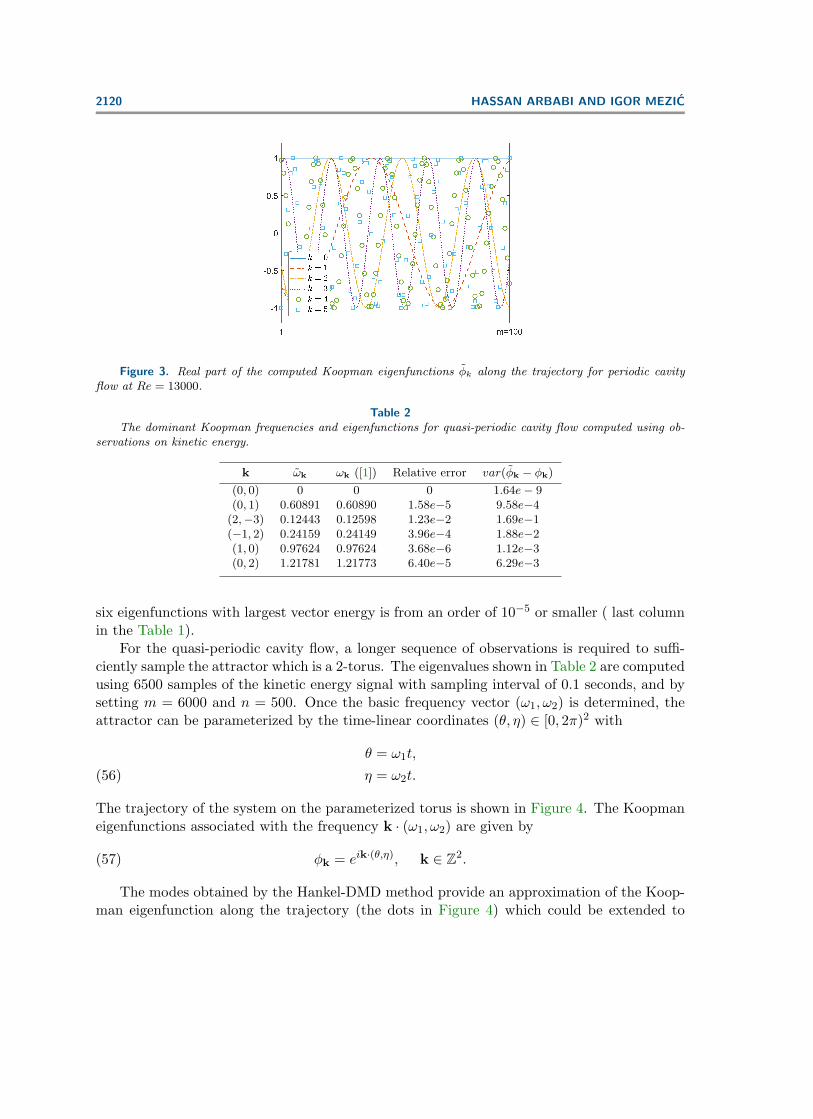
The real part of the Koopman eigenfunctions φk computed via the Hankel-DMD method areshown along the trajectory in Figure 3. The mean squared error in the approximation of the


Figure 3. Real part of the computed Koopman eigenfunctions φk along the trajectory for periodic cavityflow at Re = 13000.

Table 2The dominant Koopman frequencies and eigenfunctions for quasi-periodic cavity flow computed using ob-

servations on kinetic energy.

k ωk ωk ([1]) Relative error var(φk − φk)(0, 0) 0 0 0 1.64e− 9(0, 1) 0.60891 0.60890 1.58e−5 9.58e−4

(2,−3) 0.12443 0.12598 1.23e−2 1.69e−1(−1, 2) 0.24159 0.24149 3.96e−4 1.88e−2(1, 0) 0.97624 0.97624 3.68e−6 1.12e−3(0, 2) 1.21781 1.21773 6.40e−5 6.29e−3

six eigenfunctions with largest vector energy is from an order of 10−5 or smaller ( last columnin the Table 1).

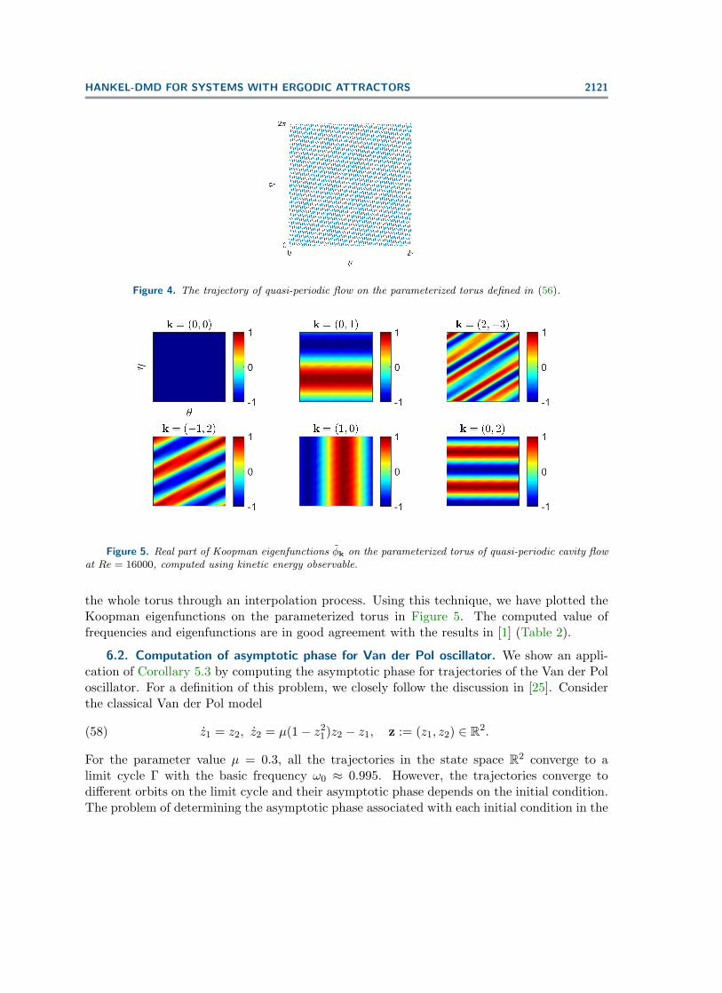
For the quasi-periodic cavity flow, a longer sequence of observations is required to suffi-ciently sample the attractor which is a 2-torus. The eigenvalues shown in Table 2 are computedusing 6500 samples of the kinetic energy signal with sampling interval of 0.1 seconds, and bysetting m = 6000 and n = 500. Once the basic frequency vector (ω1, ω2) is determined, theattractor can be parameterized by the time-linear coordinates (θ, η) ∈ [0, 2π)2 with

θ = ω1t,

η = ω2t.(56)

The trajectory of the system on the parameterized torus is shown in Figure 4. The Koopmaneigenfunctions associated with the frequency k · (ω1, ω2) are given by

φk = eik·(θ,η), k ∈ Z2.(57)

The modes obtained by the Hankel-DMD method provide an approximation of the Koop-man eigenfunction along the trajectory (the dots in Figure 4) which could be extended to


Figure 4. The trajectory of quasi-periodic flow on the parameterized torus defined in (56).

Figure 5. Real part of Koopman eigenfunctions φk on the parameterized torus of quasi-periodic cavity flowat Re = 16000, computed using kinetic energy observable.

the whole torus through an interpolation process. Using this technique, we have plotted theKoopman eigenfunctions on the parameterized torus in Figure 5. The computed value offrequencies and eigenfunctions are in good agreement with the results in [1] (Table 2).

6.2. Computation of asymptotic phase for Van der Pol oscillator. We show an appli-cation of Corollary 5.3 by computing the asymptotic phase for trajectories of the Van der Poloscillator. For a definition of this problem, we closely follow the discussion in [25]. Considerthe classical Van der Pol model

z1 = z2, z2 = µ(1− z21)z2 − z1, z := (z1, z2) ∈ R2.(58)

For the parameter value µ = 0.3, all the trajectories in the state space R2 converge to alimit cycle Γ with the basic frequency ω0 ≈ 0.995. However, the trajectories converge todifferent orbits on the limit cycle and their asymptotic phase depends on the initial condition.The problem of determining the asymptotic phase associated with each initial condition in the


state space is of great importance, e.g., in analysis and control of oscillator networks that arisein biology (see, e.g., [44, 8]). The Koopman eigenfunctions provide a natural answer for thisproblem: if φ0 is the Koopman eigenfunction associated with ω0, the initial conditions lyingon the same level set of φ0 converge to the same orbit and will have the same asymptotic phase[25]. The methodology developed in [25] is to compute the Koopman eigenfunction by takingthe Fourier (or harmonic) average of a typical observable which requires prior knowledge ofω0.

We use a slight variation of the Hankel-DMD algorithm to compute the basic (Koopman)frequency of the limit cycle and the corresponding eigenfunction φ0 in the same computation.Consider two trajectories of (58) starting at initial conditions z1 = (4, 4) and z2 = (0, 4). Theobservable that we use is f(z) = z1 + z2, sampled at every 0.1 second over a time intervalof 35 seconds (m = 250 and n = 100). Recall from Remark 1 that we can use variousvectors of ergodic sampling with the Hankel-DMD algorithm to compute the spectrum andeigenfunctions of the Koopman operator. We populate the Hankel matrices with observationson both trajectories, such that the lth column of the Hankel matrix, denoted by H l, is givenby

H l = [f(z1), f(z2), f T (z1), f T (z2), . . . , f Tm−1(z1), f Tm−1(z2)]T .

Similarly,

UH l = [f T (z1), f T (z2), f T 2(z1), f T 2(z2), . . . , f Tm(z1), f Tm(z2)]T .

The dynamic modes obtained by applying the exact DMD to these Hankel matrices approxi-mate the Koopman eigenfunctions along the two trajectories in the form of

φ0(z1, z2) := [φ0(z1), φ0(z2), φ0 T (z1), φ0 T (z2), . . . , φ0 Tm−1(z1), φ0 Tm−1(z2)]T .

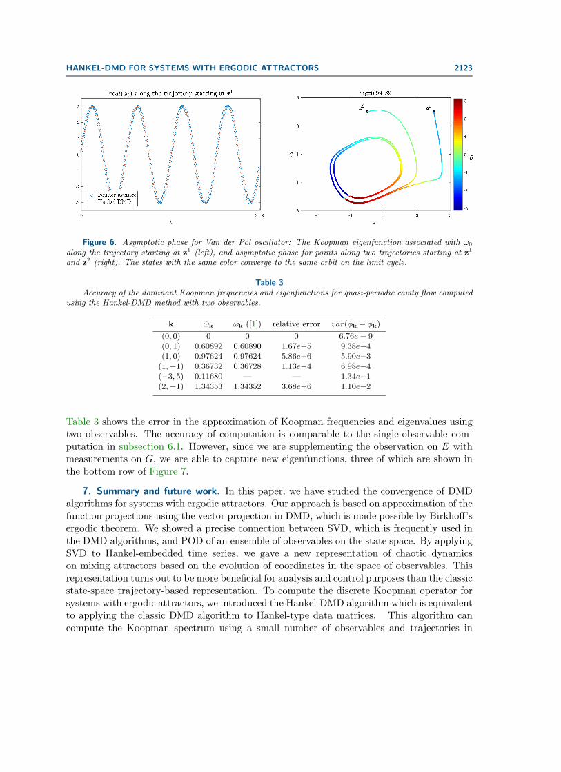
Figure 6 shows the agreement between the Hankel-DMD and the Koopman eigenfunctionsobtained from Fourier averaging with known frequency [25]. The right panel shows θ = ∠φ0plotted as the color field along the trajectories which characterizes the asymptotic phase ofeach point on the trajectories.

6.3. Application to multiple observables: The quasi-periodic cavity flow. We showthe application of Algorithm 4 with multiple observables by revisiting the example of quasi-periodic flow in subsection 6.1. Let Gi := G(t0 + i∆t) be the set of measurements of thestream function at a point on the flow domain (x = y = 0.3827 in the domain defined in [1]).Also let E be the kinetic energy of the flow. We use the Hankel matrices of observations onG and E, by setting m = 6000 and n = 500, and form the data matrices

X =[HE αHG

], Y =

[UHE αUHG

],(59)

where we have approximated the scaling factor α by

α =‖Gm‖‖Em‖

.(60)


Figure 6. Asymptotic phase for Van der Pol oscillator: The Koopman eigenfunction associated with ω0

along the trajectory starting at z1 (left), and asymptotic phase for points along two trajectories starting at z1

and z2 (right). The states with the same color converge to the same orbit on the limit cycle.

Table 3Accuracy of the dominant Koopman frequencies and eigenfunctions for quasi-periodic cavity flow computed

using the Hankel-DMD method with two observables.

k ωk ωk ([1]) relative error var(φk − φk)(0, 0) 0 0 0 6.76e− 9(0, 1) 0.60892 0.60890 1.67e−5 9.38e−4(1, 0) 0.97624 0.97624 5.86e−6 5.90e−3

(1,−1) 0.36732 0.36728 1.13e−4 6.98e−4(−3, 5) 0.11680 — — 1.34e−1(2,−1) 1.34353 1.34352 3.68e−6 1.10e−2

Table 3 shows the error in the approximation of Koopman frequencies and eigenvalues usingtwo observables. The accuracy of computation is comparable to the single-observable com-putation in subsection 6.1. However, since we are supplementing the observation on E withmeasurements on G, we are able to capture new eigenfunctions, three of which are shown inthe bottom row of Figure 7.

7. Summary and future work. In this paper, we have studied the convergence of DMDalgorithms for systems with ergodic attractors. Our approach is based on approximation of thefunction projections using the vector projection in DMD, which is made possible by Birkhoff’sergodic theorem. We showed a precise connection between SVD, which is frequently used inthe DMD algorithms, and POD of an ensemble of observables on the state space. By applyingSVD to Hankel-embedded time series, we gave a new representation of chaotic dynamicson mixing attractors based on the evolution of coordinates in the space of observables. Thisrepresentation turns out to be more beneficial for analysis and control purposes than the classicstate-space trajectory-based representation. To compute the discrete Koopman operator forsystems with ergodic attractors, we introduced the Hankel-DMD algorithm which is equivalentto applying the classic DMD algorithm to Hankel-type data matrices. This algorithm cancompute the Koopman spectrum using a small number of observables and trajectories in


Figure 7. Real part of Koopman eigenfunctions φk on the parameterized torus of quasi-periodic cavity flowat Re = 16000, computed using two observables: kinetic energy and stream function.

high-dimensional systems like fluid flows. The Hankel-DMD method also shows promise forcomputing the dissipative eigenvalues of the Koopman operator, i.e., eigenvalues inside theunit circle. We will discuss this in future articles.

Time series data and MATLAB codes. The time-series data and MATLAB codes of thenumerical examples can be found at https://mgroup.me.ucsb.edu/resources.

Acknowledgments. H.A. thanks Nithin Govindararjan for his comments on the initialmanuscript. The authors are also grateful to the anonymous reviewers for their helpful com-ments and questions.

REFERENCES

[1] H. Arbabi and I. Mezic, Study of Dynamics in Unsteady Flows using Koopman Mode Decomposition,preprint, http://arxiv.org/abs/1704.00813, 2017.

[2] B. W. Brunton, L. A. Johnson, J. G. Ojemann, and J. N. Kutz, Extracting spatial–temporal coherentpatterns in large-scale neural recordings using dynamic mode decomposition, J. Neurosci. Methods,258 (2016), pp. 1–15.

[3] S. L. Brunton, B. W. Brunton, J. L. Proctor, E. Kaiser, and J. N. Kutz, Chaos as an inter-mittently forced linear system, Nature Comm., 8 (2017), 19.

[4] S. L. Brunton, B. W. Brunton, J. L. Proctor, and J. N. Kutz, Koopman invariant subspacesand finite linear representations of nonlinear dynamical systems for control, PloS One, 11 (2016),e0150171.

[5] S. L. Brunton, J. L. Proctor, and J. N. Kutz, Compressive sampling and dynamic mode decompo-sition, J. Comput. Dyn., 2 (2015), pp. 165–191.

[6] M. Budivsic, R. Mohr, and I. Mezic, Applied Koopmanism, Chaos, 22 (2012), 047510.[7] K. K. Chen, J. H. Tu, and C. W. Rowley, Variants of dynamic mode decomposition: Boundary

condition, Koopman, and Fourier analyses, J. Nonlinear Sci., 22 (2012), pp. 887–915.[8] P. Danzl, J. Hespanha, and J. Moehlis, Event-based minimum-time control of oscillatory neuron

models, Biol. Cybern., 101 (2009), pp. 387–399.

https://mgroup.me.ucsb.edu/resources

http://arxiv.org/abs/1704.00813


[9] J.-P. Eckmann and D. Ruelle, Ergodic theory of chaos and strange attractors, Rev. Modern Phys., 57(1985), p. 617.

[10] M. Georgescu and I. Mezic, Building energy modeling: A systematic approach to zoning and modelreduction using Koopman mode analysis, Energy Buildings, 86 (2015), pp. 794–802.

[11] M. Ghil, M. Allen, M. Dettinger, K. Ide, D. Kondrashov, M. Mann, A. W. Robertson,A. Saunders, Y. Tian, F. Varadi, and P. Yiou, Advanced spectral methods for climatic timeseries, Rev. Geophys., 40 (2002), 3.

[12] D. Giannakis, Data-driven spectral decomposition and forecasting of ergodic dynamical systems, Appl.Comput. Harmon. Anal., to appear.

[13] P. R. Halmos, Lectures on Ergodic Theory, Mathematical Society of Japan, Tokyo, 1956.[14] A. C. Hansen, Infinite-dimensional numerical linear algebra: Theory and applications, in R. Soc. Lond.

Proc. A: Math. Phys. Eng. Sci., 466 (2010), pp. 3539–3561.[15] P. Holmes, J. L. Lumley, G. Berkooz, and C. Rowley, Turbulence, Coherent Structures, Dynamical

Systems and Symmetry, 2nd ed., Cambridge University Press, Cambridge, 2012.[16] J.-N. Juang and R. S. Pappa, An eigensystem realization algorithm for modal parameter identification

and model reduction, J. Guidance Control Dyn., 8 (1985), pp. 620–627.[17] S. Klus, P. Koltai, and C. Schutte, On the numerical approximation of the Perron-Frobenius and

Koopman operator, J. Comput. Dyn., 3 (2016), pp. 51–79.[18] B. O. Koopman, Hamiltonian systems and transformation in Hilbert space, Proc. Natl. Acad. Sci. USA,

17 (1931), pp. 315–318.[19] B. O. Koopman and J. von Neumann, Dynamical systems of continuous spectra, Proc. Natl. Acad.

Sci. USA, 18 (1932), pp. 255–263.[20] U. Krengel and A. Brunel, Ergodic Theorems, De Gruyter Stud. Math. 6, De Gruyter, Berlin, 1985.[21] J. N. Kutz, X. Fu, and S. L. Brunton, Multiresolution dynamic mode decomposition, SIAM J. Appl.

Dyn. Syst., 15 (2016), pp. 713–735.[22] E. N. Lorenz, Deterministic nonperiodic flow, J. Atmos. Sci., 20 (1963), pp. 130–141.[23] S. Luzzatto, I. Melbourne, and F. Paccaut, The Lorenz attractor is mixing, Commun. Math. Phys.,

260 (2005), pp. 393–401.[24] B. MacCluer, Elementary Functional Analysis, Grad. Texts in Math. 253, Springer, New York, 2008.[25] A. Mauroy and I. Mezic, On the use of Fourier averages to compute the global isochrons of (quasi)

periodic dynamics, Chaos, 22 (2012), 033112.[26] A. Mauroy and I. Mezic, Global stability analysis using the eigenfunctions of the Koopman operator,

IEEE Trans. Automat. Control, 61 (2016), pp. 3356–3369.[27] I. Mezic, Spectral properties of dynamical systems, model reduction and decompositions, Nonlinear Dy-

nam., 41 (2005), pp. 309–325.[28] I. Mezic, On applications of the spectral theory of the Koopman operator in dynamical systems and control

theory, in Proceedings of the 2015 IEEE 54th Annual Conference on Decision and Control (CDC),IEEE, Piscataway, NJ, 2015, pp. 7034–7041.

[29] I. Mezic, Koopman Operator Spectrum and Data Analysis, preprint, http://arxiv.org/abs/1702.07597,2017.

[30] I. Mezic and A. Banaszuk, Comparison of systems with complex behavior, Phys. D, 197 (2004), pp. 101–133.

[31] I. Mezic and F. Sotiropoulos, Ergodic theory and experimental visualization of invariant sets inchaotically advected flows, Phys. Fluids, 14 (2002), pp. 2235–2243.

[32] K. Petersen, Ergodic Theory, Cambridge University Press, Cambridge, 1995.[33] J. L. Proctor, S. L. Brunton, and J. N. Kutz, Dynamic mode decomposition with control, SIAM J.

Appl. Dyn. Syst., 15 (2016), pp. 142–161.[34] C. Rowley, I. Mezic, S. Bagheri, P. Schlatter, and D. Henningson, Spectral analysis of nonlinear

flows, J. Fluid Mech., 641 (2009), pp. 115–127.[35] Y. Saad, Numerical Methods for Large Eigenvalue Problems, Rev. ed., SIAM, Philadelphia, 2011.[36] T. Sauer, J. A. Yorke, and M. Casdagli, Embedology, J. Stat. Phys., 65 (1991), pp. 579–616.[37] P. Schmid and J. Sesterhenn, Dynamic mode decomposition of numerical and experimental data, in

Sixty-First Annual Meeting of the APS Division of Fluid Dynamics, 2008.

http://arxiv.org/abs/1702.07597


[38] P. J. Schmid, Dynamic mode decomposition of numerical and experimental data, J. Fluid Mech., 656(2010), pp. 5–28.

[39] R. Singh and J. Manhas, Composition Operators on Function Spaces, North Hollad Math. Stud. 179,North Holland, Amsterdam, 1993.

[40] L. Sirovich, Turbulence and the dynamics of coherent structures part I: Coherent structures, Quart.Appl. Math., 45 (1987), pp. 561–571.

[41] Y. Susuki and I. Mezic, Nonlinear Koopman modes and coherency identification of coupled swing dy-namics, IEEE Trans. Power Systems, 26 (2011), pp. 1894–1904.

[42] Y. Susuki and I. Mezic, A prony approximation of Koopman mode decomposition, in Proceedings of the2015 54th IEEE Conference on Decision and Control (CDC), IEEE, Piscataway, NJ, 2015, pp. 7022–7027.

[43] F. Takens, Detecting strange attractors in turbulence, in Dynamical Systems ad Turbulence, LectureNotes in Math. 898, Springer, Berln, 1981, pp. 368–381.

[44] S. R. Taylor, R. Gunawan, L. R. Petzold, and F. J. Doyle III, Sensitivity measures for oscillatingsystems: Application to mammalian circadian gene network, IEEE Trans. Automat. Control, 53(2008), pp. 177–188.

[45] L. N. Trefethen and D. Bau, III, Numerical Linear Algebra, Vol. 50, SIAM, Philadelphia, 1997.[46] J. H. Tu, C. W. Rowley, D. M. Luchtenburg, S. L. Brunton, and J. N. Kutz, On dynamic mode

decomposition: Theory and applications, J. Comput. Dyn., 1 (2014), pp. 391–421.[47] P. Van Overschee and B. De Moor, Subspace Identification for Linear Systems: Theory-

Implementation-Applications, Kluwer, Boston, 1996.[48] M. O. Williams, I. G. Kevrekidis, and C. W. Rowley, A data-driven approximation of the Koopman

operator: Extending dynamic mode decomposition, J. Nonlinear Sci., 25 (2015), pp. 1307–1346.[49] L. Young, What are SRB measures, and which dynamical systems have them?, J. Stat. Phys., 108 (2002),

pp. 733–754.

Ergodic Theory, Dynamic Mode Decomposition, and ...harbabi/research/M112523.pdf · Ergodic Theory,...

Documents

Transcript of Ergodic Theory, Dynamic Mode Decomposition, and ...harbabi/research/M112523.pdf · Ergodic Theory,...