High Resolution Mesh Convergence Propertiesand Parallel Efficiency of a Spectral Element

Atmospheric Dynamical Core

To appear, IJHPCA special issue on ClimateModeling Algorithms and Software Practice,

2005

John Dennis∗ Aime Fournier† William F. Spotz‡

Amik St.-Cyr∗ Mark A. Taylor‡§ Steve Thomas∗

Henry Tufo∗

Abstract

We first demonstrate the parallel performance of the dynamicalcore of a spectral element atmospheric model. The model uses contin-uous Galerkin spectral elements to discretize the surface of the Earth,coupled with finite differences in the radial direction. Results are pre-sented from two distributed memory, mesh interconnect supercom-puters (ASCI Red and BlueGene/L), using a two-dimensional spacefilling curve domain decomposition. Better than 80% parallel effi-ciency is obtained for fixed grids on up to 8938 processors. These

∗Scientific Computing Division, National Center for Atmospheric Research, BoulderColorado

†Department of Meteorology, College of Computer, Mathematical, Physical Sciences,University of Maryland at College Park

‡Computation, Computers, Information and Mathematics, Sandia National Laborato-ries, Albuquerque NM

§Corresponding author. email: mataylo@sandia.gov

1

2

runs represent the largest processor counts ever achieved for a geo-physical application. They show that the upcoming Red Storm andBlueGene/L supercomputers are well suited for performing global at-mospheric simulations with a 10km average grid spacing. We thendemonstrate the accuracy of the method by performing a full 3D meshrefinement convergence study, using the primitive equations to modelbreaking Rossby waves on the polar vortex. Due to the excellent par-allel performance, the model is run at several resolutions up to 36kmwith 200 levels using only modest computing resources. Isosurfacesof scaled potential vorticity (PV) exhibit complex dynamical features,e.g., a primary PV tongue, and a secondary instability causing roll-upinto a ring of five smaller sub-vortices. As the resolution is increased,these features are shown to converge while PV gradients steepen.

1 Introduction

The spectral element method is a finite element method in which a highdegree spectral method is used within each element. The method providesspectral accuracy while retaining both parallel efficiency and the geometricflexibility of unstructured finite elements grids. The method has proven accu-rate and efficient for a wide variety of geophysical problems, including globalatmospheric circulation modeling (Taylor et al., 1997, 1998; Giraldo, 2001;Thomas and Loft, 2002; Giraldo and Rosmond, 2004; Fournier et al., 2004;Thomas and Loft, 2004) ocean modeling (Haidvogel et al., 1997; Iskandaraniet al., 2002; Molcard et al., 2002; Iskandarani et al., 2003) and planetaryscale seismology (Komatitsch and Tromp, 1999, 2002). The method has un-surpassed parallel performance; it was used for earthquake modeling by the2003 Gordon Bell Best Performance winner, running on 1944 CPUs of theEarth Simulator (Komatitsch et al., 2003) and for climate modeling by a2002 Gordon Bell Award honorable mention, running on 2048 processors ofan IBM SP (Loft et al., 2001).

In this work we focus on a spectral element atmospheric climate model.The model is a prototype dynamical core for the Community AtmosphericModel (CAM) component of the Community Climate System Model (CCSM).The CCSM simulates the total earth system, coupling together atmosphere,ocean, sea ice and land surface models. The CAM consists of a dynamicalcore based on the hydrostatic primitive equations, coupled to sub-grid scalemodels of physical processes such as boundary layer turbulence, moist con-

3

vection and the effects of clouds on the radiative forcing (Kiehl and Gent,2004; Collins et al., 2004). We describe our model in Section 2 and thenin Section 3 we document its parallel performance on very large processorcounts. We use these results to demonstrate the ability of two upcomingparallel computers to run the spectral element model at a global resolutionof 10km. This is an important long term goal of DOE’s climate modelingprogram (Malone et al., 2004). In Section 4, we use the polar vortex problemto perform a high resolution mesh convergence study of the model. The abil-ity to run at the resolutions necessary to start to achieve convergence weremade possible by the parallel performance of the model.

2 Spectral Element Dynamical Cores

Our spectral element dynamical core solves the primitive equations using ahybrid η pressure vertical coordinate system (Simmons and Burridge, 1981),using the continuous Galerkin spectral element discretization for the horizon-tal directions (the surface of the sphere), and second order finite differencesin the vertical direction (Fournier et al., 2004; Thomas and Loft, 2004). Thespectral element method relies on quadrilateral elements. We use a subdi-vided inscribed cube to generate quasi-isotropic tilings of the sphere withsuch elements. An example mesh is shown in Fig. 1. To characterize thehorizontal resolution of these meshes, let M be the total number of elementsand N be the number of polynomials in each direction used within each el-ement. In the figure, M = 384. The spectral transforms performed withineach element rely on an N×N grid and thus the total horizontal resolution isspecified by N ×N ×M . The number of nodes along the equator is given by4(M/6)1/2N , and the average equatorial grid spacing in kilometers is givenby 2.45× 104M−1/2N−1.

Using a spectral element discretization on the sphere has several advan-tages for global climate modeling. First of all, handling the spherical ge-ometry presents no problem since the sphere can be tiled with quadrilateralelements of approximately the same size, thus avoiding clustering points atthe poles. Secondly, by using a local coordinate system within each element,the singularities associated with spherical coordinates can also be avoided.Additionally, for climate applications, the method can obtain the accuracyof traditional spherical harmonics based models with only a slight increasein the number of degrees of freedom (Taylor et al., 1997; Thomas and Loft,

4

2002).In what follows we present results from two models, SEAM and HOMME.

SEAM is a spectral element atmospheric model research code (Fournier et al.,2004). Most of the algorithms in SEAM have been reimplemented in NCAR’sHigh Order Multi-scale Modeling Environment (HOMME). HOMME addsmodern software engineering practices in addition to many new features andalgorithms, including advanced time stepping, discontinuous Galerkin, adap-tive mesh refinement and several domain decomposition strategies (Thomasand Loft, 2004; St-Cyr and Thomas, 2005; St-Cyr et al., 2004; Nair et al.,2004). Here we only use the simplest form of HOMME: explicit time step-ping, a continuous Galerkin treatment of the prognostic variables and quasi-isotropic conforming element meshes. In this form, the numerical results ofHOMME and SEAM are indistinguishable.

3 Parallel Scalability

Spectral element methods are well suited to modern cache-based parallelcomputers for several reasons. First, the basic data structure in the method,the spectral element, is naturally cache blocked. Secondly, due to the O(N3)cost of the spectral transforms, the method has a very low ratio of commu-nication to computation. Finally, the spectral element discretization allowsfor efficient two-dimensional domain decomposition strategies.

We demonstrate this performance by presenting results for HOMME run-ning on the IBM BlueGene/L (up to 7776 processors) and ASCI Red (up to8938 processors). We use vertical resolutions from 20 to 100 levels, and hor-izontal resolutions from 156km down to 10km. All cases use N = 8. For thebenchmark problem, we use timings from HOMME configured to run theHeld-Suarez test (Held and Suarez, 1994). The Held-Suarez tests were de-signed to allow for the intercomparison of the climate produced by differentatmospheric dynamical cores. Results from SEAM and HOMME have beenpreviously reported (Taylor et al., 1998; Thomas and Loft, 2004).

The Held-Suarez tests are also useful for benchmarking since they rep-resent the entire dynamical core of an atmospheric model such as CAM.Only the physics components (sub-grid scale models of physical processes)in CAM are not represented. CAM physics is column based, meaning thecalculations are performed using only data from the vertical column associ-ated with each element. Using an element based domain decomposition, all

5

the column physics will be performed on processor and require no additionalcommunication. Thus the addition of physics can only improve the parallelscalability of the dynamical core; however, the single processor performancewill be affected by the single processor performance of the column physicsmodels. One other difference between CAM and the Held-Suarez tests whichcan effect parallel performance is that CAM contains additional constituentswhich must be advected by the dynamical core. These prognostic variableswill have an identical parallel behavior as the prognostic variable for tem-perature, and thus they are represented in the Held-Suarez test but goingfrom one such variable to many such variables will result in a proportionalincrease in the required CPU time.

These factors show that the time-to-solution from a Held-Suarez testproblem can provide a reasonable estimate of the time-to-solution for a fullclimate simulation. For a given resolution, adding column physics and addi-tional constituents may actually increase the parallel scalability of the modeland the number of floating point operations per second. The time-to-solutionwill increase, but in the worst case only proportional to the complexity ofthe column physics and number of additional constituents. In typical climatesimulations, this increase is a factor in the range of 1.2 to 2.

3.1 Cache Blocking

The elements in the spectral element method provide a natural cache block-ing. By way of example, consider the 64 bit data storage requirement for atypical 8× 8 element with 20 vertical levels requires only 10 Kbytes of cacheper variable. One hundred such 3-D variables will fit into a typical 1 Mbytedata cache. If the data is stored in memory so as to avoid cache conflicts,then all the computations performed within an element can be done entirelyin cache. This blocking is independent of resolution since we can increasethe resolution by simply using more elements. This situation is unlike codesoptimized for vector architecture, where the natural block size and data ac-cess patterns grow with resolution. Thus a spectral element model maintainsgood performance even at high resolutions.

3.2 Domain decomposition

The most natural way to parallelize the spectral element method is to sim-ply assign several elements to each processor. Each element only needs in-

6

formation from adjacent elements, so the domain decomposition reduces toa standard graph partitioning problem. To solve this problem, we use analgorithm based on space filling curves (Dennis, 2003).

The resulting communication patterns are similar to finite difference/finiteelement methods which parallelize with the same type of domain decompo-sition. Thus the parallel efficiency of this method would be similar to theseother methods, except for the fact that the spectral element method involvescomputing high order derivatives using spectral transforms instead of loworder stencils. These computationally intensive transforms are performedwithin each element and are localized to each processor thus requiring nocommunication. The result is that for a wide range of problem sizes, num-ber of processors, and computer architectures, the parallel efficiency remainsabove 80%, for parallel decompositions as fine as two elements per proces-sor, and reasonable efficiency is obtained at the finest decomposition of oneelement per processor.

3.3 HOMME on ASCI Red

We first present results from the ASCI-Red computer at Sandia NationalLaboratories. ASCI-Red was the first of DOE’s Advanced Strategic Com-puting Initiative (ASCI) machines. It has 4510 nodes in a mesh interconnect,each with two 333 MHz Pentium II processors. In Fig. 2, we present the totalMFLOPS obtained per processor at several resolutions and processor counts.Each curve represents a fixed resolution, so that the the total amount of workwas kept constant while the processor count was increased. Data for two res-olutions includes parallel decompositions as fine as one element per processor.As can be seen in the figure, all resolutions achieve good scalability - betterthan 80% in all cases. In this range the performance fluctuates between 30and 40 MFLOPS per processor. The best performance obtained for eachresolution, along with the integration rate is given in Table 1.

ASCI Red is of interest because of Cray’s upcoming Red Storm archi-tecture. As of this writing, several Red Storm computers are being builtwith up to 10,000 Opteron processors running at 2 GHz. Red Storm wasdesigned to have the same balance between processor performance and inter-processor communications as ASCI Red, and thus we expect to obtain verysimilar scalability results on Red Storm. Initial results show the single pro-cessor performance of HOMME on a 2 GHz Opteron is better than 600MFLOPS. Thus with an 80% parallel efficiency, we expect to sustain at least

7

Resolution Processors GFLOPS Simulated days per day156km/26L 384 13 160040km/50L 6144 181 15420km/70L 8192 265 18

9.8km/100L 8936 294 1.5

Table 1: HOMME dynamical core (dry dynamics) benchmark runs on ASCI-Red

Resolution Processors GFLOPS Simulated days per day80km/20L 512 117 720071km/20L 1944 372 6500†

35km/40L 7776 1320 1100

Table 2: HOMME dynamical core benchmark runs on BlueGene/L. The rundenoted by a † included one prognostic moisture variable.

4.3 TFLOPS on 8936 processors of Red Storm. This is an integration rateof 22 simulated days per day for a 9.8km/100L resolution.

3.4 HOMME on IBM BlueGene/L

Our benchmark runs for the IBM BlueGene/L system were run on systemsat IBM Watson and Rochester, on up to 7776 processors using one processorper node and only using one of the floating-point pipelines. BlueGene/L usesa toroidal interconnect and PowerPC processors. Sustained MFLOPS perprocessor are shown in Fig. 3, for several resolutions and processor counts.Each curve represents a fixed resolution, so that the the total amount ofwork was kept constant while the processor count was increased. Data fortwo resolutions includes parallel decompositions as fine as one element perprocessor. The best performance obtained for each resolution, along with theintegration rate is given in Table 2.

BlueGene/L is of interest since IBM intends to build some very largesystems, with over 64,000 processors. Noting that the performance on the drydynamics problem is around 250 MFLOPS per processor even when runningwith as few as 2 elements per processor, we can estimate a performanceat 9.8km/100L on 49152 processors (2 elements per processor) to be 9.8TFLOPS, thus allowing an integration rate of 50 simulated days per day.

8

4 The Polar Vortex

The stratospheric polar vortex is bounded by strong potential-vorticity gra-dients which isolate polar air from lower latitudes. A phenomenon of majoratmospheric-research importance is the eventual mixing of these air masses,when the vortex is distorted by breaking planetary-scale Rossby waves. Thiswas the focus of Polvani and Saravanan (2000). In addition to that studyand those referenced therein, the importance of this phenomenon is under-scored by a number of recent studies of its various aspects, in various jour-nals. Thompson et al. (2000) studied the positive feedbacks involving ozonedestruction and other phenomena that may delay polar-vortex breakdownand enhance spring ozone loss. James et al. (2000) provided objective diag-nostics of characteristic winter polar-vortex displacements towards Europe orCanada, linked to transient dynamically induced ozone mini-holes. PlanetaryRossby-wave refraction was found by Limpasuvan and Hartmann (2000) tolink stratospheric polar-vortex strength to tropospheric annular-mode vari-ability. Finally, Koh and Plumb (2000) evaluated the crucial choice of bound-aries for computing material transport across the polar-vortex edge. All theseauthors also cite numerous other examples of this topic’s importance. Herewe document a minimally complex model for the numerical simulation ofpolar-vortex breakdown based on that presented in Polvani and Saravanan(2000), and then present results from SEAM for several different resolutionsup to 36km with 200 levels.

4.1 Initial Condition

Following Polvani and Saravanan (2000), our initial model state consists ofa gradient-flow balanced axisymmetric-vortex: at time t = 0, as a functionof longitude λ, co-latitude ϕ and pressure p, let the horizontal wind vector

u(λ, ϕ, p) = u0(ϕ, p) ≡ a0Ω0u0(ϕ, p)i,

the isobaric velocity ω(λ, ϕ, p) = 0, the surface pressure psfc(λ, ϕ) = 104Pa,the temperature

T (λ, ϕ, p) = T 0(ϕ, p) ≡ T0 −a2

0Ω20

R0

∂Φ0

∂ln p

and the geopotential

Φ(λ, ϕ, p) = g0zp + a20Ω

20Φ

0(ϕ, p),

9

where a0, Ω0 and g0 are the earth’s radius, angular frequency and gravity, iis the longitudinal unit vector, T0 = g0H0/R0 = 239.14K is the isotherm fora scale height H0 = 7km, R0 is the dry-air gas constant and zp ≡ H0 ln psfc/pis log-pressure height. The nonlinear gradient-flow balance is

∂Φ0

∂ϕ= −

(2µ + u0 tan ϕ

)u0,

where µ = sin ϕ, so the complete initial state only depends on the dimen-sionless velocity component u0, assuming

∫ 1

−1Φ0(ϕ, p)dµ = 0.

Let us now describe the initial profile as a function of (ϕ, p). Observingequatorward from ϕ = π/2, we assume the absolute vorticity

ζ ≡ 2µ− ∂u cos ϕ

∂µ(1)

is initially positive, almost constant until the vortex-edge latitude ϕv ≡ 60,where it decreases rapidly over a zone of width ∆ϕ ≡ 6, then again nearlyconstant until the surf-zone edge ϕs ≡ 35, followed by cubic-sine decreaseto zero at the equator, and solid-body rotation for ϕ ≤ 0. We impose u0

z = 0,where subscript z denotes evaluation at ϕ = ϕz ≡ 37 and any p. Theequatorward progression just described is controlled by four vertical-structurecoefficients cn(p) to be determined:

ζ0(ϕ, p) ≡

r′(µ)c1 + c2, µs ≤ µ,

2µc3 − 4µ3c4, 0 ≤ µ ≤ µs,

2M0e µ, µ ≤ 0,

(2)

where the step-like function

r′(µ) ≡ 1

2+

1

2tanh

µ− µv

∆µ, (3)

the specific absolute angular momentum from (1)

M(µ, p) ≡ 1− µ2 + u cos ϕ =

∫ 1

µ

ζ(µ′)dµ′, (4)

subscript e denotes evaluation at the equator ϕ = 0, subscripts s and vdenote evaluation at ϕs and ϕv, and ∆µ ≡ ∆ϕ cos ϕv. The coefficients cn(p)

10

are determined as follows. From (2,4) one has

M0(µ, p) =

−r(µ)c1 + (1− µ)c2, µs ≤ µ,

M0e − µ2c3 + µ4c4, 0 ≤ µ ≤ µs,

(1− µ2)M0e , µ ≤ 0,

(5)

where by (3) the hyperbolic ramp-like function

r(µ) ≡∫ µ

1

r′(µ′)dµ′ =µ− 1

2+

∆µ

2

(ln cosh

µ− µv

∆µ− ln cosh

1− µv

∆µ

).

Since ϕv > ϕz > ϕs we may immediately solve a linear system to obtain

c2 =M0

vrz −M0z rv

(1− µv)rz − (1− µz)rv

,

c1 = [(1− µv)c2 −M0v ]r−1

v .

Ensuring µ-continuity of (2,5) leads to another linear system with solution

c4 = µ−4s (M0

e −M0s )− 2−1µ−3

s ζ0s ,

c3 = (2µs)−1ζ0

s + 2µ2sc4.

Observing thatM0

z = 1− µ2z

andM0

s = −rsc1 + (1− µs)c2,

it only remains to define a0Ω0u0e ≡ −20m s−1 in order to get M0

e from (4),and then

u0v ≡ (1 + zp/ztop)u

0e

in order to get M0v from (4), where ztop is the model height. Finally, (4,5)

yields u0(ϕ, p), as shown in Fig. 4a.The initial scaled-potential-vorticity (Π) profile is shown in Fig. 4b. Π ≡

P (T, ζ)/P (T0, 2Ω0), where

P (T, ζ) ≡(

sec ϕ∂v

∂p

∂

∂λ− ∂u

∂p

∂

∂ϕ− ζ

∂

∂p

)θ(p, T )

approximates the Ertel potential vorticity in isobaric coordinates, θ(p, T ) ≡(p0/p)R0/cpT is the potential temperature and p0 = 105Pa. In fact Π thusdefined is identically the SPV of Polvani and Saravanan (2000, section 3).

11

4.2 Time-dependent forcing at the bottom

The model is forced by setting Φ at the surface for all time equal to

Φsfc(λ, ϕ, t) =

Φmax cos λ

(sin 9

2ϕ)2 (

1− e−t/τ), 40< ϕ< 80,

0, otherwise,

with decay time τ = 3d and amplitude Φmax = g0 × 800m. The forcing peaksat ϕ = 60 = ϕv, and increases monotonically in time. The effect is toinstigate upward-propagating Rossby waves.

4.3 Sponge layer at the top

Depending on ztop, spurious reflection may be prevented by adding the fol-lowing sponge-layer forcing near the model top, which amounts to Rayleighdamping of u and Newton damping of T :

∂(u, T )

∂t

∣∣∣∣sl

= ν · (u0 − u, T 0 − T ), (6)

where the damping coefficient

ν ≡

1

2+

1

2tanh

zp − zsl

∆z, zsl < ztop,

0, zsl ≥ ztop,(7)

zsl ≡ 2−1(zsl + ztop), ∆z ≡ 310

(ztop − zsl) and zsl = 45km.

4.4 Results

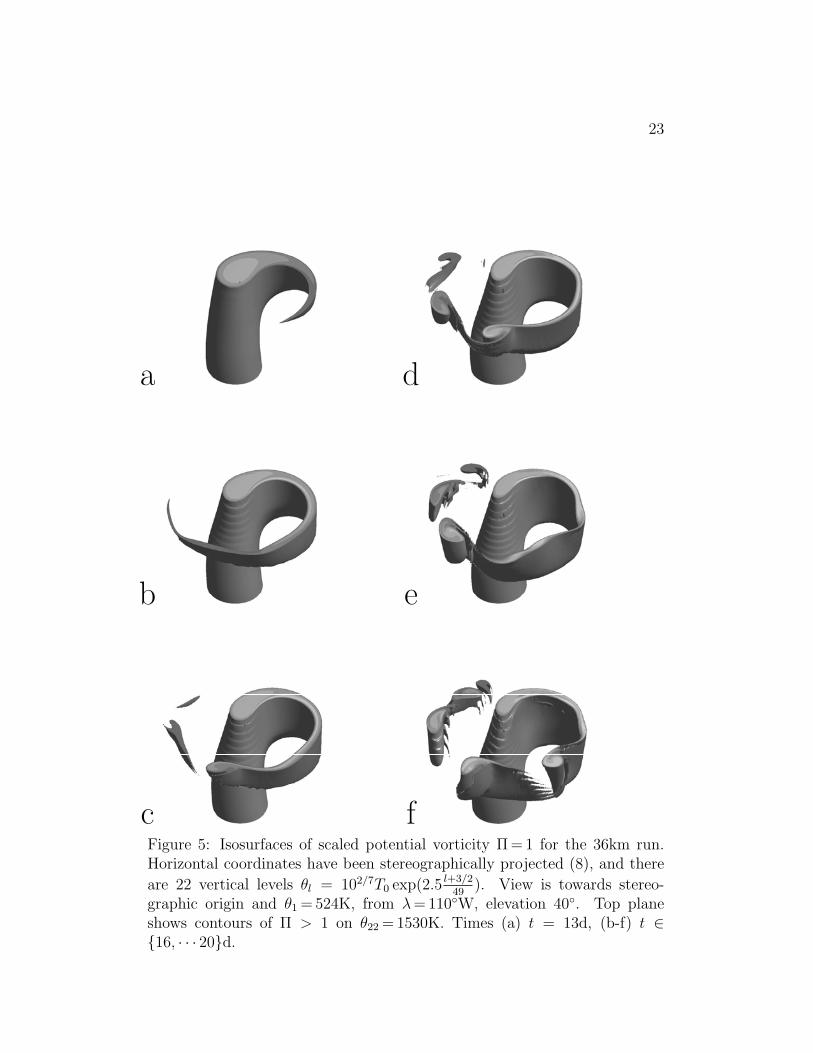
Using SEAM, we were able to carry out the polar-vortex simulation at severalresolutions, up to 36km with 200 levels. The highest resolution required≈ 105

time steps on ≈ 108 collocation points in ≈ 2 wall-clock days on 256 IBM SPRS/6000 processors. The Π isosurfaces from that run are shown in in Fig. 5.They indicate the complex dynamical features of the polar vortex: a primaryΠ “tongue,” succumbing to a secondary instability, leading to a roll-up intoa ring of five or six smaller sub-vortices.

We look at the convergence question systematically, as shown in Fig. 6. Itappears that at moderate horizontal resolution of 156km, some additional Π

12

structure is resolved in increasing from 50 to 100 levels (Fig. 6a-b), but not asmuch, from 100 to 200 levels (Fig. 6b-c). At the higher horizontal resolutionof 70km, the sub-vortices are much better resolved for 100 levels, with littlechange at 200 levels (Fig. 6d-f). Increasing the horizontal resolution to 36kmat 200 levels (Fig. 6g) produces mainly small and qualitative changes, andonly in the details, not in the overall simulation. The problem appears tohave converged w.r.t. horizontal and vertical resolution.

The precise dissipation and filtering were different for all runs, but for eachrun were empirically minimized while sufficient to stabilize the simulation.That is, we attempt to investigate the inviscid limit. This differs from otherconvergence studies in which dissipation and filtering are fixed, and onlyresolution is varied.

To investigate convergence under mesh refinement more systematically,we consider an the isentropic Π-tongue-tip position diagnostic. This may bequantified as the point xmax(θ, t) of maximum angular change β(x) of theΠ = 1 contour in stereographic projection coordinates

x ≡ tan(π/4− ϕ/2)

[cos λsin λ

]. (8)

The diagnostic involves computing the L tangent vectors tj along the Lpoints of each contour:

tj ≡ ∆

xj, j = 1,

(xj + xj−1)/2, j = 2, · · ·Lxj−1, j = L + 1,

where ∆sj ≡ sj+1 − sj. From the tj one computes the angular change

β(xj) ≡ arccos tj · tj+1 ≤ β(xmax(θ, t)), (9)

where a ≡ a/|a|. This is illustrated in Fig. 7.The area A(θ, t) enclosed by values Π ≥ 1 evolves with a qualitatively

similar pattern as resolution is increased, as shown in Fig. 8. This is agood measure of vortex erosion, as discussed in further detail by Polvaniand Saravanan (2000). We estimated A(θ, t) by summing over northern-hemisphere points with Π(λ, ϕ, θ, t) > 1:

A(θ, t) =2π

Nλ

Nϕ∑m=1

∆ sin ϕ+m

Nλ−1∑l=0

1, Π(λl, ϕm, θ, t) > 1,

0, Π(λl, ϕm, θ, t) ≤ 1,(10)

13

where λl ≡ (2N−1λ l − 1)π, ϕm ≡ (2Nϕ)−1mπ and ϕ+

m ≡ ϕm (m = 1, · · ·Nϕ),2ϕm − ϕm−1 (m = Nϕ + 1).

As an indication of convergence as resolution is increased, the ratio

s36km/s156km − 1

s150km/s300km − 1

for s = A(θ, t) stayed below 0.7 for all θ in Fig. 8, averaged over t ∈ [3, 11]d,and was usually much smaller.

5 Discussion

The spectral element method is known to perform well on parallel computers.This performance is maintained for a spectral element atmospheric model onvery large, previously unattained, processor counts. The parallel efficiencyremains between 70–80%, for parallel decompositions as fine as one elementper processor and for all problem sizes and processor counts. These resultsgive evidence that the massively parallel systems being built now (IBM’sBlueGene/L and Cray’s Red Storm ) will be able to sustain between 4-10TFLOPS of performance, allowing one to run 10km global atmospheric sim-ulations at a rate of 22–50 simulated days per day. This establishes a perfor-mance level for atmospheric modeling competitive with that obtained usingthe specialized vector supercomputer architectures of the Japanese EarthSimulator. On that machine, the AFES (Atmospheric model for the EarthSimulator) obtained 27 TFLOPS of performance and an integration rate of57 simulated days per day (Shingu et al., 2002). AFES uses a global spectralmodel for its dynamical core, and thus requires more flops to achieve similarintegration rates.

The parallel performance of the spectral element method allowed us toconduct a mesh convergence study using a polar vortex model problem. Thisproblem is the focus of much recent research. It has a complex unstableevolution dominated by strong potential-vorticity gradients. Only at highresolution (36km and 200 vertical levels) does evidence for mesh convergenceof large scale features start to become apparent.

14

6 Acknowledgments

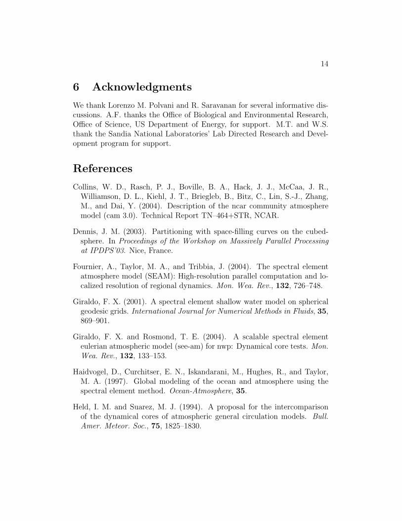
We thank Lorenzo M. Polvani and R. Saravanan for several informative dis-cussions. A.F. thanks the Office of Biological and Environmental Research,Office of Science, US Department of Energy, for support. M.T. and W.S.thank the Sandia National Laboratories’ Lab Directed Research and Devel-opment program for support.

References

Collins, W. D., Rasch, P. J., Boville, B. A., Hack, J. J., McCaa, J. R.,Williamson, D. L., Kiehl, J. T., Briegleb, B., Bitz, C., Lin, S.-J., Zhang,M., and Dai, Y. (2004). Description of the ncar community atmospheremodel (cam 3.0). Technical Report TN–464+STR, NCAR.

Dennis, J. M. (2003). Partitioning with space-filling curves on the cubed-sphere. In Proceedings of the Workshop on Massively Parallel Processingat IPDPS’03. Nice, France.

Fournier, A., Taylor, M. A., and Tribbia, J. (2004). The spectral elementatmosphere model (SEAM): High-resolution parallel computation and lo-calized resolution of regional dynamics. Mon. Wea. Rev., 132, 726–748.

Giraldo, F. X. (2001). A spectral element shallow water model on sphericalgeodesic grids. International Journal for Numerical Methods in Fluids, 35,869–901.

Giraldo, F. X. and Rosmond, T. E. (2004). A scalable spectral elementeulerian atmospheric model (see-am) for nwp: Dynamical core tests. Mon.Wea. Rev., 132, 133–153.

Haidvogel, D., Curchitser, E. N., Iskandarani, M., Hughes, R., and Taylor,M. A. (1997). Global modeling of the ocean and atmosphere using thespectral element method. Ocean-Atmosphere, 35.

Held, I. M. and Suarez, M. J. (1994). A proposal for the intercomparisonof the dynamical cores of atmospheric general circulation models. Bull.Amer. Meteor. Soc., 75, 1825–1830.

15

Iskandarani, M., Haidvogel, D., Levin, J., Curchitser, E. N., and Edwards,C. A. (2002). Multiscale geophysical modeling using the spectral elementmethod. Computing in Science and Engineering, 4.

Iskandarani, M., Haidvogel, D., and Levin, J. (2003). A three-dimensionalspectral element model for the solution of the hydrostatic primitive equa-tions. Journal of Computational Physics, 186.

James, P. M., Peters, D., and Waugh, D. W. (2000). Very low ozone episodesdue to polar vortex displacement. Tellus, 52B(4), 1123–1137.

Kiehl, J. T. and Gent, P. R. (2004). The community climate system model,version two. J. Clim., 17, 3666–3682.

Koh, T.-Y. and Plumb, R. A. (2000). Lobe dynamics applied to barotropicRossby-wave breaking. Phys. Fluids, 12(6), 1518–1528.

Komatitsch, D. and Tromp, J. (1999). Introduction to the spectral-elementmethod for 3-d seismic wave propagation. Geophys. J. Int., 139, 806–822.

Komatitsch, D. and Tromp, J. (2002). Spectral-element simulations of globalseismic wave propagation - i. validation. Geophys. J. Int., 149, 390–412.

Komatitsch, D., Tsuboi, S., Ji, C., and Tromp, J. (2003). A 14.6 billiondegrees of freedom, 5 teraflops, 2.5 terabyte earthquake simulation onthe earth simulator. In Proceedings of the ACM / IEEE SupercomputingSC’2003 conference.

Limpasuvan, V. and Hartmann, D. L. (2000). Wave-maintained annularmodes of climate variability. J. Climate, 13, 4414–4429.

Loft, R., Thomas, S., and Dennis, J. (2001). Terascale spectral elementdynamical core for atmospheric general circulation models. In Proceedingsof the ACM / IEEE Supercomputing SC’2001 conference.

Malone, R. C., Drake, J. B., Jones, P. W., and Rotman, D. A. (2004). Com-puting the climate. In A Science-based Case for Large-scale Simulation,Volume II. to appear in the SIAM series on Computational Science andEngineering. Draft available at http://www.pnl.gov/scales.

16

Molcard, A., Pinardi, N., Iskandarani, M., and Haidvogel, D. (2002). Winddriven circulation of the mediterranean sea simulated with a spectral ele-ment ocean model. Dynamics of Atmospheres and Oceans, 35.

Nair, R. D., Thomas, S., and Loft, R. (2004). A discontinuous galerkintransport scheme on the cubed-sphere. under review, Mon. Wea. Rev.

Polvani, L. M. and Saravanan, R. (2000). The three-dimensionalstructure of breaking Rossby waves in the polar wintertime strato-sphere. J. Atmos Sci., 57, 3663–3685. [Available on-line atwww.columbia.edu/ lmp/lmp pubs.html.].

Shingu, S., Takahara, H., Fuchigami, H., Yamada, M., Tsuda, Y., Ohfuchi,W., Sasaki, Y., Kobayashi, K., Hagiwara, T., Habata, S., Yokokawa, M.,Itoh, H., and Otsuka, K. (2002). A 26.58 tflops global atmospheric sim-ulation with the spectral transform method on the earth simulator. InProceedings of the ACM / IEEE Supercomputing SC’2002 conference.

Simmons, A. J. and Burridge, B. M. (1981). An energy and angular mo-mentum conserving vertical finite-difference scheme and hybrid verticalcoordinates. Mon. Wea. Rev., 109, 758–766.

St-Cyr, A. and Thomas, S. (2005). Nonlinear operator integration factorspliting for the shallow water equations. to appear, Applied NumericalMathematics.

St-Cyr, A., Dennis, J., Thomas, S., and Tufo, H. (2004). An adaptive non-conforming spectral element atmospheric model. under review, Journal ofScientific Computing.

Taylor, M., Tribbia, J., and Iskandarani, M. (1997). The spectral elementmethod for the shallow water equations on the sphere. J. Comput. Phys.,130, 92–108.

Taylor, M., Loft, R., and Tribbia, J. (1998). Performance of a spectral ele-ment atmospheric model (SEAM) on the HP Exemplar SPP2000. Techni-cal Report TN–439+EDD, NCAR.

Thomas, S. and Loft, R. (2002). Parallel semi-implicit spectral element at-mosphere model. Journal of Scientific Computing, 15.

17

Thomas, S. and Loft, R. (2004). The ncar spectral element climate dynamicalcore: Semi-implicit eulerian formulation. J. Sci. Comput.

Thompson, D. W. J., Wallace, J. M., and Hegerl, G. C. (2000). Annularmodes in the extratropical circulation. Part II: Trends. J. Climate, 13,1018–1036.

List of Figures

1 An example spectral element grid for the Earth. Continen-tal outlines are shown for reference. The grid is generated byprojecting an inscribed cube onto the surface, and then sub-dividing each of the 6 faces of the cube into an 8 × 8 grid ofelements. Typically each element uses a degree 7 polynomialexpansion. Finite differences are used in the vertical direction(not shown). . . . . . . . . . . . . . . . . . . . . . . . . . . . 19

2 Performance of the HOMME dynamical core (dry dynamics)benchmark runs on ASCI Red. Each curve shows the perfor-mance for a fixed resolution as the number of processors isincreased. . . . . . . . . . . . . . . . . . . . . . . . . . . . . . 20

3 Performance of the HOMME dynamical core (dry and moistdynamics) benchmark runs on BlueGene/L. Each curve showsthe performance for a fixed resolution as the number of pro-cessors is increased. . . . . . . . . . . . . . . . . . . . . . . . . 21

4 Initial state profiles vs latitude ϕ (, abscissa). (a) Zonal-wind isotachs (m s−1) vs log-pressure height zp (km, ordinate).Contour interval is 10 m s−1 and u(ϕ = 37, zp) = 0. (b)Isopleths of scaled potential vorticity vs potential temperatureθ (K, ordinate). Contour interval is 0.2 and Π(ϕ = 0, θ) = 0. . 22

5 Isosurfaces of scaled potential vorticity Π = 1 for the 36km run.Horizontal coordinates have been stereographically projected(8), and there are 22 vertical levels θl = 102/7T0 exp(2.5 l+3/2

49).

View is towards stereographic origin and θ1 = 524K, from λ = 110W,elevation 40. Top plane shows contours of Π > 1 on θ22 = 1530K.Times (a) t = 13d, (b-f) t ∈ 16, · · · 20d. . . . . . . . . . . . 23

18

6 Stereographic projection in the the θ = 1500K surface of Π(λ, ϕ)contours from −0.3 to 1.3 by 0.1, at t = 20d. Values below0.2 are dark gray and above 0.8 are white. Resolutions (a)156km/50L, (b) 156km/100L, (c) 156km/200L; (d-f) as in (a-c) but for 70km; (g) as in (f) but for 36km. . . . . . . . . . . . 24

7 Π = 1 contours, for t ∈ 5, 7, 9, 11d (light gray to black). Di-amonds indicate xmax(θ, t) (Eq. 9). (a-d) Descending levelsθ = 3000, 2500, 2000, 1500K for 300km resolution. (e-h) As(a-d) but for 156km. (i-l) As (a-d) but for 36km. . . . . . . . 25

8 Horizontal vortex-area A(θ, t) (10) vs t (d, abscissa) for (a)θ = 3000, (b) 2500, (c) 2000, (d) 1500K. Resolutions are300km/48L (light gray), 156km/48L (gray) and 36km/200L(dark gray). . . . . . . . . . . . . . . . . . . . . . . . . . . . . 26

19

Figure 1: An example spectral element grid for the Earth. Continentaloutlines are shown for reference. The grid is generated by projecting aninscribed cube onto the surface, and then subdividing each of the 6 faces ofthe cube into an 8×8 grid of elements. Typically each element uses a degree7 polynomial expansion. Finite differences are used in the vertical direction(not shown).

20

156km L26, 384 elements 40km L50, 6144 elements 20km L70, 24576 elements 10km L100, 98304 elements

1 8 64 512 4096 32768NCPU

0

10

20

30

40

50

MFL

OPS

per

CPU

Figure 2: Performance of the HOMME dynamical core (dry dynamics) bench-mark runs on ASCI Red. Each curve shows the performance for a fixedresolution as the number of processors is increased.

21

80km L20, 1536 elements 71km L20, 1944 elements 35km L40, 7776 elements

1 8 64 512 4096 32768NCPU

0

100

200

300

400

MFL

OPS

per

CPU

Figure 3: Performance of the HOMME dynamical core (dry and moist dy-namics) benchmark runs on BlueGene/L. Each curve shows the performancefor a fixed resolution as the number of processors is increased.

22

−20

0

20

40

60

80

100

120

10 20 30 40 50 60 70 80

5

10

15

20

25

30

35

40

45

50

55 a

φ (°)

z p (km

)

0.2

0.4

0.6

0.8

1

1.2

1.4

1.6

1.8

2

10 20 30 40 50 60 70 80

1000

1500

2000

2500

3000

3500

4000

4500 b

φ (°)

θ (K

)

Figure 4: Initial state profiles vs latitude ϕ (, abscissa). (a) Zonal-windisotachs (m s−1) vs log-pressure height zp (km, ordinate). Contour intervalis 10 m s−1 and u(ϕ = 37, zp) = 0. (b) Isopleths of scaled potential vorticityvs potential temperature θ (K, ordinate). Contour interval is 0.2 and Π(ϕ =0, θ) = 0.

23

a

b

c

d

e

fFigure 5: Isosurfaces of scaled potential vorticity Π = 1 for the 36km run.Horizontal coordinates have been stereographically projected (8), and there

are 22 vertical levels θl = 102/7T0 exp(2.5 l+3/249

). View is towards stereo-graphic origin and θ1 = 524K, from λ = 110W, elevation 40. Top planeshows contours of Π > 1 on θ22 = 1530K. Times (a) t = 13d, (b-f) t ∈16, · · · 20d.

24

a

b

c

d

e

f g

Figure 6: Stereographic projection in the the θ = 1500K surface of Π(λ, ϕ)contours from −0.3 to 1.3 by 0.1, at t = 20d. Values below 0.2 are dark grayand above 0.8 are white. Resolutions (a) 156km/50L, (b) 156km/100L, (c)156km/200L; (d-f) as in (a-c) but for 70km; (g) as in (f) but for 36km.

25

−0.6−0.4−0.2 0 0.2 0.4−0.6

−0.4

−0.2

0

0.2

0.4

0.6d

−0.6

−0.4

−0.2

0

0.2

0.4

0.6c

−0.6

−0.4

−0.2

0

0.2

0.4

0.6b

−0.6

−0.4

−0.2

0

0.2

0.4

0.6a

−0.6−0.4−0.2 0 0.2 0.4

h

g

f

e

−0.6−0.4−0.2 0 0.2 0.4

l

k

j

i

Figure 7: Π = 1 contours, for t ∈ 5, 7, 9, 11d (light gray to black).Diamonds indicate xmax(θ, t) (Eq. 9). (a-d) Descending levels θ =3000, 2500, 2000, 1500K for 300km resolution. (e-h) As (a-d) but for 156km.(i-l) As (a-d) but for 36km.

26

0 1 2 3 4 5 6 7 8 9 10 11

0.75

0.8

0.85

0.9

d

0.75

0.8

0.85

0.9

c

0.75

0.8

0.85

0.9

b

0.75

0.8

0.85

0.9

a

Figure 8: Horizontal vortex-area A(θ, t) (10) vs t (d, abscissa) for (a) θ =3000, (b) 2500, (c) 2000, (d) 1500K. Resolutions are 300km/48L (light gray),156km/48L (gray) and 36km/200L (dark gray).