H. Lim et al- Chaos, Transport, and Mesh Convergence for Fluid Mixing

8/3/2019 H. Lim et al- Chaos, Transport, and Mesh Convergence for Fluid Mixing

http://slidepdf.com/reader/full/h-lim-et-al-chaos-transport-and-mesh-convergence-for-fluid-mixing 1/23

Chaos, Transport, and Mesh Convergence for Fluid Mixing∗

H. Lim,1 Y. Yu,1 J. Glimm,1, 2 X.-L. Li,1 and D. H. Sharp3

1Department of Applied Mathematics and Statistics,

Stony Brook University, Stony Brook, NY 11794-3600, USA

2 Computational Science Center, Brookhaven National Laboratory, Upton, NY 11793-6000, USA

3 Los Alamos National Laboratory, Los Alamos, NM

(Dated: January 30, 2008)

Chaotic mixing of distinct fluids produces a convoluted structure to the inter-

face separating these fluids. For miscible fluids (as considered here), this interface is

defined as a 50% mass concentration isosurface. For shock wave induced (Richtmyer-

Meshkov) instabilities, we find the interface to be increasingly complex as the com-

putational mesh is refined. This interfacial chaos is cut off by viscosity, or by the

computational mesh if the Kolmogorov scale is small relative to the mesh. In a regime

of converged interface statistics, we then examine mixing, i.e. concentration statis-

tics, regularized by mass diffusion. For Schmidt numbers significantly larger than

unity, typical of a liquid or dense plasma, additional mesh refinement is normally

needed to overcome numerical mass diffusion and to achieve a converged solution of

the mixing problem. However, with the benefit of front tracking and with an algo-

rithm that allows limited interface diffusion, we can assure convergence uniformly in

the Schmidt number. We show that different solutions result from variation of the

Schmidt number. We propose subgrid viscosity and mass diffusion parameterizations

which might allow converged solutions at realistic grid levels.

PACS numbers: 47.27.wj, 47.27.tb, 47.27.-i

Keywords: Schmidt number, Mass Diffusion, Turbulence, Multiphase flow



2

I. INTRODUCTION

A. Overview

Acceleration driven turbulent mixing is a classical hydrodynamical instability, in which

acceleration is directed across a fluid interface separating distinct fluids of different

densities23. We are concerned here with impulsive acceleration produced by a shock

wave passing through the fluids. This problem is known as the Richtmyer-Meshkov

(RM) instability. We consider a circular geometry, with a converging circular shock at

the outer edge, and inside this, two fluids separated by a perturbed circular interface.

The problem was previously described in detail12,14,26. We consider the problem in two

dimensions, in order to pursue conveniently issues of mesh refinement. Initial and late

time simulation density plots are shown in Fig. 1.

The fluid interface, at late time, is volume filling. The transport coefficients (viscosity,

mass diffusion, and heat conductivity) are given dimensionlessly as the Reynolds number

Re = UL/ν , the Schmidt number Sc = ν/µ, and the Prandtl number P r = ν/κ.

Here ν is the kinematic viscosity, µ the mass diffusivity and κ the thermal diffusion rate.

Throughout this paper, thermal diffusion is set to zero. U and L are characteristic velocity

and length scales. Dilute gases have Schmidt numbers of the order of unity or smaller,

while liquids and dense plasmas typically have larger Schmidt numbers. We show that

the solution depends on the Schmidt number. With under resolved physical transport

mechanisms, their numerical analogues (numerical mass diffusion, heat conduction and

numerical or artificial viscosity) play the role of the missing or under resolved physical

variables, and select the solution. Computer codes then apparently converge to one of

the nonunique solutions.

The ability of the microphysics at the smallest turbulent scales (and those below

this scale, limited by a diffusive length scale) to affect the macroscopic flow occurs with

turbulent combustion18, where details of atomic level mixing affect stoichiometry and

temperature, thus the local flame speeds and the macroscopic flow. From the point of



3

FIG. 1: Initial (left) and late time (right) density plot for the Richtmyer-Meshkov fluid insta-

bility under study in this paper.

view of turbulent combustion, a converged solution should yield a converged probability

density function (pdf), as a function of space and time, for the joint distribution of thespecies concentrations and the temperature. The sensitive dependence of the temperature

and species concentration pdfs is interface related and is amplified by the chaotic nature

of the volume filling interface.



4

B. The Flow Instability Problem

In the problem considered here, see Fig. 1, the flow is dominated by a single strong

shock wave, starting at the outer edge of the computational domain (a half circle). The

shock passes through the interface separating the two fluids, proceeds to the origin, re-

flects there and expands outward, recrossing the interface region and finally exiting at the

outer boundary. The interface region, due to the shock induced instability, expands into

a mixing zone, which has a very complex structure. Especially after the second passage

of the shock (the reshock or reflected shock passage), the mixing zone becomes highlychaotic. The inner and outer edges of the mixing zone are defined in terms of 5% and

95% volume fraction contours, after a spatial average over the circular symmetry vari-

able. The mixing zone is then defined as the region between these inner and outer edges.

The software which captures the space time trajectory of these waves in the numerical

solution is known as a wave filter7,8,26. A space time plot of the shock trajectories and

mixing zone edges is shown in Fig. 2.

The numerical solutions are by the front tracking FronTier algorithm6

. This algo-rithm uses a Godunov finite difference solver based on the MUSCL algorithm 4,24, and a

sharp (tracked) interface to eliminate, or optionally13, to limit mass diffusion across the

interface. Thus the FronTier numerical Schmidt number is ∞, and it allows simulation

of any desired (physical) Schmidt or Prandtl number. From the point of view of tur-

bulence modeling, the simulations can be described as under resolved or resolved direct

numerical simulation (DNS). Specifically, no subgrid algorithms are used to represent the

unresolved scales.

In order to explore grid and convergence effects on simulated turbulence and mixing in

high Schmidt number flows, we artificially specify non-physical (high) values for viscosity.

In this way we explore the range of convergence to DNS for a single problem.

We have already observed11 that the interface for the problem under study is chaotic,

with length proportional to ∆x−1, with respect to its mesh (non) convergence (i.e. rate of

divergence) properties. This fact is demonstrated in Fig. 3, where the length / area ratio



5

Radius

T i m e

0 5 10 15 20

0

2 0

4 0

6 0

8 0

1 0 0

1 2 0

FIG. 2: Space time (r, t) contours of the primary waves, as detected by the wave filter algorithm.

These are the inward (direct) and outward (reflected) shock waves and the inner and outer

edges of the mixing zone, all detected within a single rotational averaging window, in this case

θ ∈ [−45o, 0o].

is shown in physical units (left frame) and mesh units (right frame); transport coefficients

have been set to zero.

From Fig. 3, we observe that somewhat after reshock, the interface length, in mesh

units, occupies a constant ratio to the mesh area of the mixing zone. We call this ratio

the mesh level surface fraction. Its value is approximately time independent (about

30%), after a transient period following the second shock passage. We note here and

in many later plots, some lost of mesh level complexity in the finest grid simulations.

Further mesh refinement studies will be needed to determine the evolution of mesh level



6

time

i n t e r f a c e l e n g t h / m i x i n g z o n e v o l u m e

0 20 40 60 80 100 1200

5

10

15

20

200 x 400

400 x 800

800 x 1600

1600 x 3200

time

g r i d

l e n g t h / g r i d

a r e a

0 20 40 60 80 100 1200

0.2

0.4

0.6

200 x 400

400 x 800

800 x 1600

1600 x 3200

FIG. 3: Plot of the interface length divided by the mixing zone area vs. time. Left: Length

and volume measured in physical units. Right: Length and volume measured in mesh units

([physical length / physical area] ×∆x). Results for four mesh levels are displayed.

complexity under continued mesh refinement. In any case, at the grid levels attained

here, the interface is mesh volume filling, cutoff by the mesh, and highly complex or

chaotic in nature.

C. Organization of Paper

The goal of this paper is to study mixing at the atomic scale, and its dependence

on transport parameters (viscosity and diffusivity). According to conventional ideas,

viscosity15 (after a time delay2 for the initiation of turbulence) limits the vorticity at high

wave numbers. At high Schmidt numbers, and at still higher wave numbers, the scaling

exponent for the concentration fluctuations is predicted to change from an Obukov-

Corrsin exponent to a lower Batchelor exponent1,22, before being suppressed by mass

diffusion. These ideas form the basis of the stretched vortex subgrid model10,21. Presum-

ably, there will be a time delay for the applicability1 of the Batchelor spectrum, which is

based on an assumed statistically steady state theory for the concentration fluctuations.

We follow a different approach to this problem, based on DNS to determine the con-



7

centration pdfs for converged solutions and to parameterize diffusive subgrid models for

large eddy simulations (LES). In this sense, our program can be related to conventional

ideas in the modeling of turbulence18. In Sec. II, we explore the role of viscosity to limit

the velocity fluctuations and small scale eddies. The Atwood number of the flow is de-

fined as A = (ρ2 − ρ1)/(ρ2 + ρ1). Initially A = 0.72 while at time of reshock, A ≈ 0.26.

This non negligible value for A indicates that density fluctuations couple into the fluid

equations, and thus that the concentration is not accurately regarded as a passive scalar.

We report evidence of mesh convergence of the statistics describing interfacial complex-

ity and the fine scale features of the mix, for simulations in a DNS regime. Evidence

indicating a sensitivity of temperature to details of physical and numerical modeling for

the flow problem considered here was reported earlier12,14. Sec. III studies mass diffusion

to determine the concentration pdfs. A final Sec. IV contains some speculations regard-

ing mathematical existence theories and comments regarding subgrid models to allow

converged calculations on realistic meshes.

II. TURBULENCE, CUTOFFS AND MESH CONVERGENCE

We set a (time dependent) length scale L to be the width of the mixing zone, and

the velocity scale U to be the turbulent velocity U = δv2. The angle brackets · · ·

denote an angular (or in principle ensemble) average. We also define Remesh = U ∆x/ν .

The Kolmogorov scale is λK = (ν 3/)1/4 . Here is the dissipation rate,

=ν

2

S ij 22 , (1)

where S ij is the strain rate tensor,

S ij =1

2

∂ui

∂x j+

∂u j∂xi

. (2)

We plot Re and the mesh Kolmogorov scale λK mesh = λK /∆x vs. Remesh for the sim-

ulations analyzed here, in Fig 4. The condition λK mesh ≥ 1 is generally taken as the

definition of a DNS.



8

Remesh

R e

10-1

100

101

102

103

104

100

101

102

103

104

105

106

200x400

400x800800x1600

1600x3200

Remesh

λ K m e s h

10-1

100

101

102

103

104

10-3

10-2

10-1

100

101

200x400

400x800800x1600

1600x3200

FIG. 4: Left: Re vs. Remesh at t = 90 for several mesh levels. Right: λK mesh vs. Remesh. Both

plots are virtually independent of Sc for the range of Sc considered. Some of the simulations

at each grid level are resolved below the Kolmogorov scale, and are resolved DNS. Others, on

the route to resolution, are under resolved DNS.

A. Convergence of Macroscopic Flow Observables

The objective here is to compute the large scale solution features accurately. This

includes the trajectories of the principal waves, as illustrated in Fig. 2, and other macro

solution features, such as the mean densities and velocities of each phase within each

homogeneous solution region between the principal waves. This objective is related to

the systematic convergence study carried out earlier26. In that study, we found statis-

tical convergence for many mean flow variables, to define what we call the macroscopic

description of the flow. In Fig. 5, we plot the relative wave error defined in terms of

the mixing zone edge positions, for a variety of mesh levels and transport coefficients.

The error (or discrepancy) is determined by comparison of the simulation to a fine grid

(3200× 1600) simulation having zero transport coefficients. The reported discrepancy is

thus a mixture of mesh errors (except for the finest grid) and discrepancies associated

with modification of the transport coefficients from a nominal value (zero).

We consider convergence in this macro sense as a function of Remesh for each value of

∆x. From Fig. 5, we see that for the three grid levels shown, the smallest converged value



9

Remesh

r e l a t i v e w a v e e r r o r

10-1

100

101

102

103

104

0

0.05

0.1

0.15

0.2

400x800 Sc=0.1

400x800 Sc=1

400x800 Sc=10

800x1600 Sc=0.1

800x1600 Sc=1

800x1600 Sc=10

1600x3200 Sc=0.1

1600x3200 Sc=1

1600x3200 Sc=10

FIG. 5: Time integrated relative errors in the mixing zone edge locations as compared to a fine

grid, zero transport simulation.

of Remesh progresses from about 30 to 2 as the mesh is refined. Some of the simulations

shown (coarse grids, to the far left of Fig. 5) are clearly not convergent and are eliminated

from subsequent analysis. With a macro converged simulation having Remesh = 2, we turn

to Fig. 4 and observe that on the finest grid, the corresponding λK mesh = 2, indicating

that the simulation is clearly DNS.

To examine in more detail the effects of modified transport on the accuracy of the

simulation, as compared to an ideal case with zero transport, we consider in Table I

a range of additional variables. We consider mean density and radial velocity data.

The mean angular velocity is essentially zero. Energy data is not presented, as it was

observed12,14 that temperature is sensitive to details of numerical and physical modeling;

we expect a similar dependence for energy. Energy and temperature will be considered

in a separate study in which the Prandtl number plays a role.

We consider Sc = 10 but not Sc = 1.0 or Sc = 0.1. The density and velocity

distributions depend on the Schmidt number, and the high Schmidt number cases are

the most comparable to the ideal case (computed with ideal parameters, i.e. with zero

numerical mass diffusion). Since any physical problem must have a finite Schmidt number



10

and other transport coefficients, the discrepancy between the ideal (zero transport) and

the finite Schmidt simulations probably reflects ideal simulation errors compared to an

(infeasible) DNS simulation with molecular values for the transport coefficients. We

cannot fully determine which of the two solutions is “better”. We only present data

showing that the difference is small for Sc = 10.

We consider separately the errors in the mixed regions and the single phase regions,

singly or doubly shocked. Each simulation thus defines five regions in space time, to be

analyzed separately, with boundaries as illustrated in Fig. 2. Comparing two simulations,

we consider the space time points which lie in a common region for both simulations.

Call these points R, and call the fluid variable v, with v1 and v2 the variables to be

compared between the two simulations. Then the discrepancy is defined as R|v1 − v2|dxdt R|v1|dxdt

, (3)

where v1 refers to the ideal simulation. The twice shocked heavy fluid is nearly stationary,

so that the velocities are small and the denominator in (3) is small. Thus the large

relative error in Table I for this variable reflects relatively large differences between small

quantities.

From Table I and Fig. 5, we conclude that our strategy of forcing a DNS simulation by

an artificial increase of the viscosity does not seriously degrade the simulation accuracy

with regard to the macro variables. Its effect could be compared to computing with a

somewhat coarser mesh, and since the mesh is already rather fine, the resulting solutions

appear to be acceptable as far as macro variable convergence is concerned. We regard the

modified transport parameters as turbulent viscosity coefficients in a Smagorinsky type

LES subgrid model. In this sense, we describe these simulations as converged LES or as

DNS relative to the modified transport parameters. The benefit is a possibly converged

study of the micro variables.



11

Re 5 × 102 3 × 103 3 × 104 4 × 105

Once shocked pure

phase heavy density 0.005 0.001 0.0003 0.0001

Twice shocked pure

phase heavy density 0.02 0.01 0.01 0.01

Once shocked pure

phase light density 0.02 0.008 0.002 0.0007

Twice shocked purephase light density 0.03 0.01 0.008 0.007

Mixed phase density 0.06 0.03 0.02 0.02

Once shocked pure

phase heavy velocity 0.02 0.005 0.001 0.0005

Twice shocked pure

phase heavy velocity 0.71 0.39 0.26 0.33

Once shocked pure

phase light velocity 0.09 0.03 0.004 0.0008

Twice shocked pure

phase light velocity 0.17 0.07 0.03 0.03

Mixed phase velocity 0.20 0.08 0.04 0.04

Shock position 0.06 0.02 0.003 0.002

TABLE I: Relative discrepancy: fine grid Sc = 10 solutions compared to an ideal simulation

with zero transport, for a series of error measures.

B. Convergence of the Interface Length

A second objective of our simulations, to be addressed in Sec. III, is to investigate fine

scale level mixing properties, including mass fraction concentration pdfs for the distinct



12

species of the mixtures. In preparation for Sec. III, we study here statistical measures

related to convergence of the interface. The basic result is that DNS, with λK ≥ ∆x

(λK mesh ≥ 1), show convergence of statistics measuring fine scale interface properties.

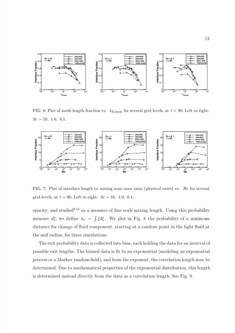
Our first result concerns the mesh length fraction. The ratio, as defined by Fig. 3, right

frame, for a fixed time t = 90, is plotted in Fig. 6 for a range of simulations with a

large range of viscosities and mass diffusivities. The ratio is largely independent of the

Schmidt number and is also mainly independent of Reynolds number and the Kolmogorov

scale for λK mesh ≤ 0.5, namely for the under resolved DNS range. For these simulations,

approximately 30% of the mesh blocks have a unit of interface length. This statement

is independent of mesh for the range of simulations explored here. With more mesh

resolution, i.e. larger values of λK mesh, the simulations are in transition to a DNS. In

this case the chaotic development of the interface appears to be limited, in that mesh

refinement with no other change of parameters (which will increase λK mesh, decrease

Remesh but not influence Re) also decreases the mesh length fraction.

The mesh related scaling of Fig. 6 is useful for understanding the under resolved

DNS range of simulations, where the simulations are chaotic and growing new fine scale

features at each level of mesh refinement. The data collapse onto a single curve. For the

DNS regime, however, it is more convenient to use physical units, with mesh dependence

and convergence clearly displayed. For this purpose, we replot the same data in Fig. 7.

With this scaling, we can observe the convergence of the interface length for the DNS

range of simulations. Convergence occurs more rapidly for smaller Schmidt numbers and

for smaller Reynolds numbers. For Sc = 0.1 and the finest mesh shown, convergence

appears to occur at Reynolds numbers near 4000.

C. An Interfacial Correlation Length Scale

We introduce a correlation length scale λC to characterize the microstructure of mix.

The correlation length is defined in terms of the probability of exit distance ξ from a

given phase or mean distance to the complementary phase, introduced19,20 for models of



13

x

xxxx

xxx

x

λKmesh

I n t e r f a c e

F r a c t i o n

10-3

10-2

10-1

100

101

0

0.1

0.2

0.3

0.4

0.5

200x400

400x800

800x1600

1600x3200

x

Sc = 10t = 90

x

xxxxx

xx

x

λKmesh

I n t e r f a c e

F r a c t i o n

10-3

10-2

10-1

100

101

0

0.1

0.2

0.3

0.4

0.5

200x400

400x800

800x1600

1600x3200

x

Sc = 1t = 90

x

xxx

xxxx

λKmesh

I n t e r f a c e

F r a c t i o n

10-3

10-2

10-1

100

101

0

0.1

0.2

0.3

0.4

0.5

200x400

400x800800x1600

1600x3200

x

Sc = 0.1t = 90

FIG. 6: Plot of mesh length fraction vs. λK mesh for several grid levels, at t = 90. Left to right:

Sc = 10, 1.0, 0.1.

xx x x x x x x x

Re

I n t e r f a c e

F r a c t i o n

100

101

102

103

104

105

106

0

5

10

15

20

200x400

400x800

800x1600

1600x3200

xSc = 10

t = 90

xx x x x x x x x

Re

I n t e r f a c e

F r a c t i o n

100

101

102

103

104

105

106

0

5

10

15

20

200x400

400x800

800x1600

1600x3200

xSc = 1

t = 90

xx x x x x x x

Re

I n t e r f a c e

F r a c t i o n

100

101

102

103

104

105

106

0

5

10

15

20

200x400

400x800

800x1600

1600x3200

xSc = 0.1

t = 90

FIG. 7: Plot of interface length to mixing zone area ratio (physical units) vs. Re for several

grid levels, at t = 90. Left to right: Sc = 10, 1.0, 0.1.

opacity, and studied9,12 as a measure of fine scale mixing length. Using this probability

measure dξ, we define λC =

ξdξ . We plot in Fig. 8 the probability of a minimum

distance for change of fluid component, starting at a random point in the light fluid at

the mid radius, for three simulations.

The exit probability data is collected into bins, each holding the data for an interval of

possible exit lengths. The binned data is fit to an exponential (modeling an exponential

process or a Markov random field), and from the exponent, the correlation length may be

determined. Due to mathematical properties of the exponential distribution, this length

is determined instead directly from the data as a correlation length. See Fig. 9.



14

length

p r o b a b i l i t y

d e n s i t y

0 0.1 0. 2 0.3 0. 4 0.5 0. 6 0.7 0. 8 0.9 110

-2

10-1

100

101

length


d e n s i t y

0 0.1 0. 2 0.3 0. 4 0.5 0. 6 0.7 0. 8 0.9 110

-2

10-1

100

101

length


d e n s i t y

0 0.1 0. 2 0.3 0. 4 0.5 0. 6 0.7 0. 8 0.9 110

-2

10-1

100

101

FIG. 8: Probability of minimum exit distance from the light phase, starting at a random light

fluid point on the mid radius. The dashed line in each frame is the plot of the best fit exponential

distribution. Three DNS, left to right, Sc = 10, 1, 0.1.

Remesh

λ C m e s h

10-1

100

101

102

103

104

0

2

4

6

8

10

12

400x800 Sc=0.1

400x800 Sc=1

400x800 Sc=10

800x1600 Sc=0.1

800x1600 Sc=1

800x1600 Sc=10

1600x3200 Sc=0.1

1600x3200 Sc=1

1600x3200 Sc=10

Re

λ C

102

103

104

105

106

0

0.05

0.1

0.15

0.2

0.25

0.3

0.35

400x800 Sc=0.1

400x800 Sc=1

400x800 Sc=10

800x1600 Sc=0.1

800x1600 Sc=1

800x1600 Sc=10

1600x3200 Sc=0.1

1600x3200 Sc=1

1600x3200 Sc=10

FIG. 9: Left: plot of λC /∆x vs. Remesh for a range of transport parameters and mesh levels,

at t = 90. Right: the same data replotted as λC vs. Re.

We can now assess interface convergence in terms of the behavior of λC . For the under

resolved regime, we look at the large Remesh limit of the left frame of Fig. 9. In this regime,λC mesh has a nearly constant value (about 2), independent of mesh and Schmidt number.

As noted earlier, the finest grids display some loss of grid level complexity. For the DNS

regime, we look at the smaller Reynolds numbers in the right frame of Fig. 9. This limit

also suggests convergence, to an Sc dependent limit, as we expect.

λC can be thought of as a mean bubble or droplet radius for two phase flow having



16

Remesh

e x p o n e n t i a l m o d e l e r r o r

10-1

100

101

102

103

104

0

0.2

0.4

0.6

0.8

1

400x800 Sc=0.1400x800 Sc=1

400x800 Sc=10

800x1600 Sc=0.1

800x1600 Sc=1

800x1600 Sc=10

1600x3200 Sc=0.1

1600x3200 Sc=1

1600x3200 Sc=10

FIG. 10: Plot of the exponential model error for a range of transport parameters and mesh

levels, at t = 90.

Remesh

λ D

/ λ C

10-1

100

101

102

103

104

-2

0

2

4

6

8

10

12

400x800 Sc=10

800x1600 Sc=10

1600x3200 Sc=10

Remesh

λ D

/ λ C

10-1

100

101

102

103

104

-2

0

2

4

6

8

10

12

400x800 Sc=1

800x1600 Sc=1

1600x3200 Sc=1

Remesh

λ D

/ λ C

10-1

100

101

102

103

104

-2

0

2

4

6

8

10

12

400x800 Sc=0.1

800x1600 Sc=0.1

1600x3200 Sc=0.1

FIG. 11: The ratio λD/λC vs. Remesh for several mesh levels and for Sc = 10, 1.0, 0.1.

this ratio vs. Remesh in Fig. 11 for a variety of Schmidt numbers and meshes. To analyze

this figure, we discuss separately the small and large Remesh asymptotes. The latter is

the under resolved regime. In this regime, λD/λC is independent of the Schmidt number,

and has a value below 1, indicating little opportunity for mass diffusion to occur. In

contrast, the small Remesh limit in this figure represents the DNS. These are strongly

dependent on Sc. They appear to be converged to a grid independent value.



17

Light fluid mixture fraction

P r o b a b i l i t y d e n s i t y

0 0.1 0. 2 0.3 0. 4 0.5 0. 6 0.7 0. 8 0.9 10

1

2

3

4

5

6

θ = 0.11λ

D/λC = 0.98



0 0.1 0. 2 0.3 0. 4 0.5 0. 6 0.7 0. 8 0.9 10

1

2

3

4

5

6

θ = 0.23λ

D/λC = 3.29



0 0.1 0. 2 0.3 0. 4 0.5 0. 6 0.7 0. 8 0.9 10

1

2

3

4

5

θ = 0.38λ

D/λC = 5.25

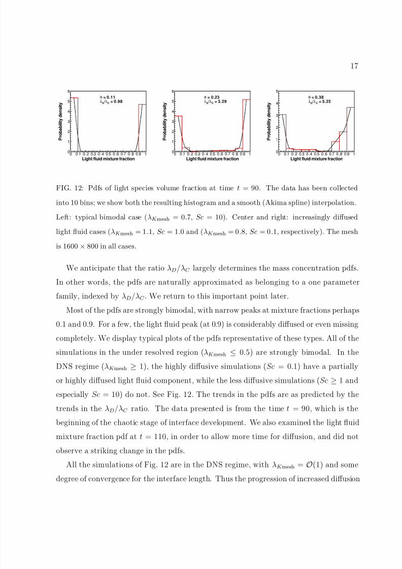
FIG. 12: Pdfs of light species volume fraction at time t = 90. The data has been collected

into 10 bins; we show both the resulting histogram and a smooth (Akima spline) interpolation.

Left: typical bimodal case (λK mesh = 0.7, Sc = 10). Center and right: increasingly diffused

light fluid cases (λK mesh = 1.1, Sc = 1.0 and (λK mesh = 0.8, Sc = 0.1, respectively). The mesh

is 1600 × 800 in all cases.

We anticipate that the ratio λD/λC largely determines the mass concentration pdfs.

In other words, the pdfs are naturally approximated as belonging to a one parameter

family, indexed by λD/λC . We return to this important point later.Most of the pdfs are strongly bimodal, with narrow peaks at mixture fractions perhaps

0.1 and 0.9. For a few, the light fluid peak (at 0.9) is considerably diffused or even missing

completely. We display typical plots of the pdfs representative of these types. All of the

simulations in the under resolved region (λK mesh ≤ 0.5) are strongly bimodal. In the

DNS regime (λK mesh ≥ 1), the highly diffusive simulations (Sc = 0.1) have a partially

or highly diffused light fluid component, while the less diffusive simulations (Sc ≥ 1 and

especially Sc = 10) do not. See Fig. 12. The trends in the pdfs are as predicted by thetrends in the λD/λC ratio. The data presented is from the time t = 90, which is the

beginning of the chaotic stage of interface development. We also examined the light fluid

mixture fraction pdf at t = 110, in order to allow more time for diffusion, and did not

observe a striking change in the pdfs.

All the simulations of Fig. 12 are in the DNS regime, with λK mesh = O(1) and some

degree of convergence for the interface length. Thus the progression of increased diffusion



18

observed in Fig. 12 reflects a change in the physical formulation of the problem, namely

an approximate 10 fold increase in mass diffusion with each successive frame, and is not

related to mesh convergence or subgrid modeling issues.

To understand the greater sensitivity of the light fluid peak than the heavy peak to

mass diffusion, we note that the result of diffusing heavy fluid into a region of light fluid

can easily make a large change in the mass weighted mixture fraction, while the diffusion

of the same fraction of light fluid into a region of heavy fluid will have a relatively smaller

effect.

The mean molecular mixing fraction θ, defined25 as

θ =f 1f 2

f 1 f 2(5)

is a common measure of mixing. Here f k is the mass concentration fraction for the species

k. With Sc = ∞, obviously there will be zero mass diffusion, and θ = 0. The probability

distribution function for the species concentrations f i is a more refined measure of mixing,

and provides the level of detail needed for prediction of turbulent combustion. In each

frame of Fig. 12, the values of θ = θ(rmid) on the mid radius of the mixing zone and

λD/λC are indicated. θ depends sensitively on the grid resolution for the under resolved

regime. In the DNS regime it depends on the transport coefficients but should be mesh

independent. The values of θ we report are smaller than those commonly reported for

simulation studies of mixing, especially for Rayleigh-Taylor mixing.

IV. A MATHEMATICAL AND COMPUTATIONAL FOOTNOTE

A. Mathematical Existence and Uniqueness Theories

If it is true that numerical solutions to the Euler equations are underdetermined,

and that the convergence process produces new structures on each length scale, what is

the consequence of these facts for a mathematical existence theory for these equations?

It would appear that if such a mathematical solution were to exist, it might not be



19

a function, but a generalized function in the sense of compensated compactness. The

compensated compactness generalized functions are pdfs depending on space and time,

not dissimilar from what is observed computationally. In the one dimensional existence

theory of compensated compactness of DiPerna16,17 and Ding and co-workers3,5, the first

and easier step is to show existence of the generalized solution. The more difficult second

step is to show that a generalized solution is a classical (weak) one. In view of the

slow rate of progress with the existence theory in two dimensions, and in view of the

possibility that this second step might not be correct, it is worth trying to establish

generalized compensated compactness solutions without the step of passing to a classical

one. Typically such proofs are based on compactness, a method of proof which yields

existence but not uniqueness for the weak solutions. We have already commented on

the possible nonuniqueness of solutions to the Euler equations. We also note that weak

solutions in the form of a space time dependent pdf for the primitive variables are actually

what is required scientifically for a combustion simulation. For this reason, such pdf

weak solutions couple into the requirements of computational physics, whether they are

required as a fundamental scientific truth or not.

B. A Practical LES Subgrid Model

We also speculate on the consequences of the ideas expressed here for practical simula-

tions of fluid mixing. We start by recalling the two types of objectives for the simulations.

The first, which we call macro objectives, are to obtain locations of the principal waves

and mean flow quantities in agreement with a fine grid simulation having minimal or zerotransport coefficients. The comparison simulations have viscosity and mass diffusion co-

efficients set to the molecular values or as modified by turbulent subgrid models. The

second objective is to obtain converged values for the joint pdfs of temperature and mass

concentration of the mixing species. Since these pdfs appear to depend on the physical

choice of the transport coefficients, the convergence algorithm must be parameterized

to be consistent with the physics. We call this the micro objective. Both are required



20

within a single simulation.

To attain these two goals, and a third goal of practical or feasible levels of simulation,

we are proposing two different classes of simulations. The purpose of the first is to

obtain, to the extent possible, direct knowledge of the micro observables. Here we allow

artificially high levels of viscosity, as long as the macro variables are in approximate

agreement with the reference solution. For such simulations, the interface appears to

have converged, and we use molecular values of the Schmidt number to set values of the

coefficient of mass diffusion. Continued mesh refinement should lead to stable values for

the micro variables. We anticipate a one parameter family of concentration pdfs as the

Schmidt number or the ratio λD/λC is varied. This is a conjecture which has still be

verified.

If we manage in this manner to obtain converged values for the micro observables,

we then move to our second class of simulations. For this class of simulations, we set

the physical viscosity to its molecular value, perhaps as modified by a subgrid model to

account for the influence of the unresolved scales on those being computed. With the

knowledge of the concentration pdfs from the first class of simulations, we can also adjust

the mass diffusion coefficient in the second class of simulations to give micro observables

in agreement with the first. To achieve this agreement, we depend on the conjecture that

the concentration pdfs lie approximately on a one parameter family, which can be indexed

by the mass diffusion (i.e., the Schmidt number or the ratio λD/λC ). Here the grids can

be notable coarser, and the simulations should be readily feasible. This program appears

to be consistent with accepted ideas in turbulence modeling18.

In future work, we hope to fill in the gaps in this program and establish the practicalityof simulations which are converged in both their micro and macro observables.

∗ This work was supported in part by U.S. Department of Energy grants DE-AC02-98CH10886

and DE-FG52-06NA26208, and the Army Research Office grant W911NF0510413. The sim-



21

ulations reported here were performed in part on the Galaxy linux cluster in the Department

of Applied Mathematics and Statistics, Stony Brook University, and in part on New York

Blue, the BG/L computer operated jointly by Stony Brook University and BNL. Los Alamos

National Laboratory Preprint LA-UR-08-0068.

1 G. Batchelor. The Theory of Homogeneous Turbulence. The University Press, Cambridge,

1955.

2 William Cabot and Andrew Cook. Reynolds number effects on Rayleigh-Taylor instability

with possible implications for type Ia supernovae. Nature Physics, 2:562–568, 2006.

3 G.-Q. Chen. Convergence of the Lax-Friedrichs scheme for isentropic gas dynamics III. Acta

Mathematica Scienitia , 6:75–120, 1986.

4 P. Colella. A direct Eulerian MUSCL scheme for gas dynamics. SIAM Journal on Computing ,

6(1):104–117, 1985.

5 X. Ding, G.-Q. Chen, and P. Luo. Convergence of the Lax-Friedrichs scheme for isentropic

gas dynamics I and II. Acta Mathematica Scientia , 5:415–432, 433–472, 1985.

6 Jian Du, Brian Fix, James Glimm, Xicheng Jia, Xiaolin Li, Yunhua Li, and Lingling Wu.

A simple package for front tracking. J. Comp. Phys., 213:613–628, 2006. Stony Brook

University preprint SUNYSB-AMS-05-02.

7 S. Dutta, E. George, J. Glimm, J. Grove, H. Jin, T. Lee, X. Li, D. H. Sharp, K. Ye, Y. Yu,

Y. Zhang, and M. Zhao. Shock wave interactions in spherical and perturbed spherical

geometries. Nonlinear Analysis, 63:644–652, 2005. University at Stony Brook preprint

number SB-AMS-04-09 and LANL report No. LA-UR-04-2989.

8

J. Glimm, J. W. Grove, Y. Kang, T. Lee, X. Li, D. H. Sharp, Y. Yu, K. Ye, and M. Zhao.Statistical Riemann problems and a composition law for errors in numerical solutions of shock

physics problems. SISC , 26:666–697, 2004. University at Stony Brook Preprint Number SB-

AMS-03-11, Los Alamos National Laboratory number LA-UR-03-2921.

9 J. Glimm, J. W. Grove, X. L. Li, W. Oh, and D. H. Sharp. A critical analysis of Rayleigh-

Taylor growth rates. J. Comp. Phys., 169:652–677, 2001.



22

10 D. J. Hill, C. Pantano, and D. L. Pullin. Large-eddy simulation and multiscale modeling of

a Richtmyer-Meshkov instability with reshock. J. Fluid Mech , 557:29–61, 2006.

11 H. Lee, H. Jin, Y. Yu, and J. Glimm. On the validation of turbulent mixing simulations

of Rayleigh-Taylor mixing. Phys. Fluids, 2007. Accepted for publication. Stony Brook

University Preprint SUNYSB-AMS-07-03.

12 H. Lim, Y. Yu, H. Jin, D. Kim, H. Lee, J. Glimm, X.-L. Li, and D. H. Sharp. Multi scale

models for fluid mixing. Special issue CMAME , 2007. Accepted for publication. Stony Brook

University Preprint SUNYSB-AMS-07-05.

13 X. F. Liu, Y. H. Li, J. Glimm, and X. L. Li. A front tracking algorithm for limited mass

diffusion. J. of Comp. Phys., 2007. Accepted. Stony Brook University preprint number

SUNYSB-AMS-06-01.

14 T. O. Masser. Breaking Temperature Equilibrium in Mixed Cell Hydrodynamics. Ph.d. thesis,

State University of New York at Stony Brook, 2007.

15 A. S. Monin and A. M. Yaglom. Statistical Fluid Mechanics: Mechanics of Turbulence. MIT

Press, 1971.

16 R. Di Perna. Convergence of approximate solutions to conservation laws. Arch. Rational

Mech. Anal., 82:27–70, 1983.

17 R. Di Perna. Compensated compactness and general systems of conservation laws. Trans.

Amer. Math. Soc., 292:383–420, 1985.

18 Heintz Pitsch. Large-eddy simulation of turbulent combustion. Annual Rev. Fluid Mech.,

38:453–482, 2006.

19

G. C. Pomraning.Linear kinetic theory and particle transport in stochastic mixtures

, vol-ume 7 of Series on Advances in Mathematics for Applied Sciences. World Scientific, Singa-

pore, 1991.

20 G. C. Pomraning. Transport theory in discrete stochastic mixtures. Advances in Nuclear

Science and Technology , 24:47–93, 1996.

21 D. Pullin. A vortex based model for the subgrid flux of a passive scalar. Phys. of Fluids,



23

12:2311–2319, 2000.

22 D. Pullin and T. S. Lundgren. Axial motion and scalar transport in stretched spiral vortices.

Phys. of Fluids, 13:2553–2563, 2001.

23 D. H. Sharp. An overview of Rayleigh-Taylor instability. Physica D , 12:3–18, 1984.

24 P. Woodward and P. Colella. Numerical simulation of two-dimensional fluid flows with strong

shocks. J. Comp. Phys., 54:115, 1984.

25 D. L. Youngs. Three-dimensional numerical simulation of turbulent mixing by Rayleigh-

Taylor instability. Phys. Fluids A, 3:1312–1319, 1991.

26 Y. Yu, M. Zhao, T. Lee, N. Pestieau, W. Bo, J. Glimm, and J. W. Grove. Uncertainty

quantification for chaotic computational fluid dynamics. J. Comp. Phys., 217:200–216, 2006.

Stony Brook Preprint number SB-AMS-05-16 and LANL preprint number LA-UR-05-6212.

H. Lim et al- Chaos, Transport, and Mesh Convergence for Fluid Mixing

Documents

Transcript of H. Lim et al- Chaos, Transport, and Mesh Convergence for Fluid Mixing