High-Power 7 MHz Bandpass Filter - K0ZR –...

Copyright J.E. Crawford 2017

K0ZR December 1, 2016

High-Power 7 MHz Bandpass Filter

Introduction

I began building my station’s SO2R capability two years ago. In addition to the automatic-switching Hamation

Bandpass filters on each radio, I have tuned coaxial stubs to reduce harmonics just prior to going to the antennas.

This function is desirable in that while affording additional strong signal immunity, it also serves to reduce any

harmonics emanating from each amplifier. Obviously, the stubs must operate near the 1,500 watt level.

There are several referencesi available which accurately point out the sensitivity of a stub implementation to its

placement along the transmission line. In short, if the stub is attached at a high-impedance point on the line, it can

offer, singly, around 25 dB of additional attenuation to the harmonic for which it is designed. This will deteriorate

as the stub’s placement is located at lower and lower impedance points along the transmission line.

I want to have immunity from stub placement on the line while also offering considerably more attenuation to all

frequencies other than the desired pass frequency. Toward that end I designed and constructed a sixth order

elliptic bandpass filter described herein.

Background on Design Process

Today there are multiple, automated filter synthesis

programs available. For my design I utilized ELSIEii

which is available “free” for filters up to 7th order.

For higher order filters one must purchase a license

for ~ $100. ELSIE will synthesize Butterworth,

Chebyshev, Elliptic, and Gaussian filters, in lowpass,

highpass, or bandpass configurations. This design is

a 6th order Cauer (elliptic) bandpass filter.

There are several commercially available filters like

this filter, however they range in price from ~ $300

(Amplifiers, Filters, Antennas in the UK) each to as

much as $500 (DX Engineering). This adds up quickly

across six different HF amateur bands. This fact, plus

the fact I enjoy designing and building filters, I

elected to go the “homebrew” route.

When operating at the 1,500 watt level, simple

calculations reveal very quickly the importance of

minimizing loss. Only 0.3 dB insertion loss leads to

100 watts dissipated in the filter. This loss, and the

accompanying heat, is our enemy. The heat, if

allowed to grow too large, will skew the filter’s

passband, leading to more loss, and in a worst case,

eventual destruction of the filter. From a

conservative perspective, moderate heat will age the

components as well, possibly leading to premature

failure. These things need to be avoided, therefore I

strived for minimum loss.

How to Attain Minimum Loss

A number of elements enter into the loss

mechanisms in any filter. Fundamentally, theory

shows us that minimum loss is not always achieved

by using the lowest filter order deemed sufficient for

the application. This means more research on the

part of the designer is required. The actual stopband

width is crucial in that there is a “Q multiplying

effect” which if left unattended, can drive

component currents to excessively high levels. This

design uses what I considered the largest practical

passband width to reduce required element Qs.

Additionally, the diameteriii of each inductor

compared to the average inductor length was

chosen to achieve theoretical Qs exceeding 400.

This is a “must” for low insertion loss.

Other Philosophies in the Design

Cost is important to me – this is my hobby.

Doorknob and silver mica capacitors at the required

voltage ratings are not cheap these days. And, more

than likely, one must consider paralleling multiple,

smaller value capacitors in order to achieve RF

current spreading so as not to exceed the current

capability of any one capacitor. This adds cost,

possibly considerable cost. The route chosen here to

drive down the cost of capacitors is to use MLCCs:

multi-layer ceramic chip capacitors. More on the

capacitor selections follows.


While I greatly preferred a professional looking PC

board for the filter, the overall dimensions of it are

so great as to preclude obtaining a reasonable cost

commercially produced board. Therefore, I etched

my own board, using for the most part medium and

large-point magic markers to layout the copper

landscape desired. I wound each inductor before

beginning the board layout, otherwise I would not

have known the linear dimensions required to

accommodate each coil.

Each inductor is wound with #12 polypermaleze wire

available through The RF Connectioniv. In retrospect,

#14 wire would have been sufficient for the lower

current inductors.

Very integral to the overall design process is the

continual assessment of the accompanying voltages

and currents for each design. For a 1500 watt filter,

these details cannot be left out. For each design

considered, I modeled it in Simetrix, a SPICE type

program. In so doing, I was able to assess both the

voltage and current expected across/through each

component when drive with 1,500 watts. This is

very important, as only by doing this analysis can

one know where the marginal/stressing parts are in

your filter design.

All traces on the PCB are around 0.25 inches in

width. Even if this deviates the microstrip’s

impedance slightly from the desired 50 ohms, it is of

paramount importance in order to not exceed the

current density capabilities of the 1 oz. PCB used in

this design.

And finally, as will be seen, each capacitor is realized

by the paralleling of as many as 12 capacitors for

current sharing. This drives layout considerations.

And finally, the reader should ask, “Why a 6th order

filter instead of an odd-order?” For elliptic filters,

even-orders produce output impedances different

than 50 ohms. In this case the result was 48 ohms.

The reason this was done here is that L4-C4

circulating currents in the 5th order design were ~ 25

amps compared to ~ 16 amps for the 6th order.

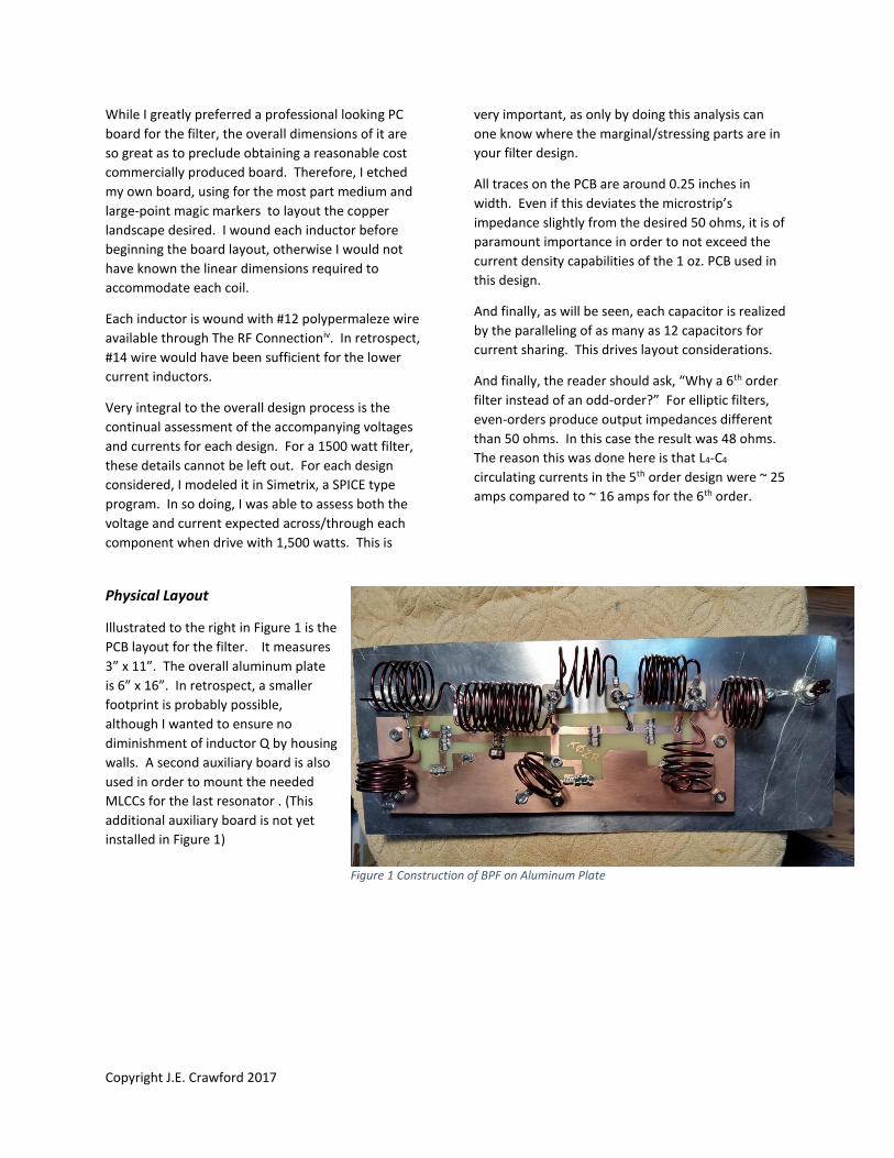
Physical Layout

Illustrated to the right in Figure 1 is the

PCB layout for the filter. It measures

3” x 11”. The overall aluminum plate

is 6” x 16”. In retrospect, a smaller

footprint is probably possible,

although I wanted to ensure no

diminishment of inductor Q by housing

walls. A second auxiliary board is also

used in order to mount the needed

MLCCs for the last resonator . (This

additional auxiliary board is not yet

installed in Figure 1)

Figure 1 Construction of BPF on Aluminum Plate


Details of the Design

Figure 2 The “Design” Window Within ELSIE

Figure 3 Passband and Stopband Response – Directly from ELSIE


Figure 4 Schematic of 6th Order BPF – Directly from ELSIE (Note each resonator’s tuned frequency)

Proceeding left-to-right in the schematic above, the associated currents for resonators 1-8 are the

following, determined from Simetrix, at 1500 W input. All voltages were less than 500 V.

Comp Amps Comp Amps

L1 6.4 L5 12.5

C1 6.4 C5 4.6

L2 10.8 L6 4.9

C2 3.0 C6 12.7

L3 3.0 L7 14.7

C3 10.9 C7 14.5

L4 17.35 L8 7.8

C4 17.3 C8 7.8 Figure 5 Table of Component Currents at 1,500 W

Miscellaneous Assembly Pictures

Left Side of Filter Right Side of Filter


Full Filter Assembly “in its box” Close-Up of Inductor Standoffs and MLCCs

Full Frequency Sweep Close-Up of 7 MHz Passband

Note the insertion loss in the left figure specifies 0.70 dB. This is considerably above the ~ 0.2 dB true

insertion loss just due to resolution on the full-scale plot.

Tuning Up the Filter

This filter is actually reasonably straight forward to tune up given its topology. Noting Figure 4, each

resonator has a “self-resonant frequency” listed. In the process of constructing the filter, I had

beginning turns numbers for each inductor, determined through use of the web-based inductance

calculator referenced in the end notes. I constructed a small PC board on which I mounted each

inductor, one at a time, and resonated it with a fixed capacitance. I would adjust the inductor until the

resonant frequency was what it should be for the amount of capacitance used; in my case 138 pF. This

was very effective in getting a good starting point for each resonator.

After complete assembly, those parallel resonators that created “zeros in transmission”, specifically

14.072, 3.6839, 11.966, and 4.332 MHz, I adjusted each respective inductor to attain the deep notches

seen in the overall transmission display. These were resonators 2,3,6, and 7. Once this was

accomplished I began iterating back and forth with the resonators to be tuned to 7.2 MHz, striving to get

the return loss I wished across the 40m band. The return loss is greater than 25 dB across the 40m

band. While at times I had the return loss even better, the overall shape of the filter was not as

“pretty”, so I went for “pretty” and said 25 dB return loss is good enough!


Miscellaneous

Trials runs with the filter began with 500 W, then proceeded to ~ 1200 W. Operating for ~ 10 minutes

with 1,200 W yielded a temperature rise in the C4 capacitors of only around 5 degrees as registered on

an IR gun temperature sensor. I operated the 2016 CQWW with the filter in place and had no problems

whatsoever. A check of the passband after the contest for signs of possible stress or over-heating

revealed all was well, and the passband remained unchanged.

One aspect of this project is selection of the MLCCs. While one can do this manually, it is much less time

consuming, and probably accurate, to get some computer help. Therefore, I surveyed what MLCCs with

breakdown voltages above 1 KV were available from Mouser. I inserted this information in a “list”

within a Python script and let it do its work. One instructs the program regarding total current through

the capacitors (obtained using Simetrix), maximum current through a single capacitor, and the total

capacitance required. The Python script then works with the available values to select those

combinations of capacitors which can be considered. In making these selections, you don’t want the

different capacitors to be too different in value, otherwise the current distribution across the capacitor

bank will be skewed, with some getting more current than desired.

For those not familiar with MLCCs, some further comments. Little information can be found, at

frequency, for the current handling capability of MLCCs. ATC MLCCs, which are very costly, come with

this information but few other manufacturers provide this. The current capacity comes down to what is

the ESR – equivalent series resistance – of the MLCC. It is this resistance, acting with the RF current

which will generate heat and potentially destroy/short the capacitor. So, to the extent possible, choose

low ESR MLCCs, larger packages to help with heat dissipation, and in my case I tried to keep the RF

current to 1.5 amps or less per MLCC.

Enter Total Capacitance : 350

Requested Maximum Current Capacity = 12

Minimum # of Capacitors to use is 8.0

# C1 # C2 Cap Range Tot Cap

1 33.0 7 47.0 14.0 362.0

2 33.0 6 47.0 14.0 348.0

3 33.0 5 47.0 14.0 334.0

2 39.0 6 47.0 8.0 360.0

3 39.0 5 47.0 8.0 352.0

4 39.0 4 47.0 8.0 344.0

5 39.0 3 47.0 8.0 336.0

5 39.0 3 56.0 17.0 363.0

6 39.0 2 56.0 17.0 346.0

5 47.0 3 33.0 14.0 334.0

6 47.0 2 33.0 14.0 348.0

7 47.0 1 33.0 14.0 362.0

3 47.0 5 39.0 8.0 336.0

4 47.0 4 39.0 8.0 344.0

5 47.0 3 39.0 8.0 352.0

6 47.0 2 39.0 8.0 360.0

2 56.0 6 39.0 17.0 346.0

3 56.0 5 39.0 17.0 363.0


Python Script

# Script to Optimize Capacitor Selection for Filter Designs # Jeff Crawford December 1, 2016 # K0ZR # import math CapList = [10, 12, 15, 18, 20, 22, 27, 30, 33, 39, 47, 56, 68, 82, 100, 110, 120, 150, 160, 180, 220, 240, 270, 300] Ia = input ('Enter Total Current, A: ') Imax = input ('Maximum Current in Each Capacitor, A: ') Ctotal = input ('Enter Total Capacitance : ') CapN = math.ceil( Ia*1.0/Imax) M = len(CapList) # Maximum number of capacitors in list to choose from # Capacitors considered are from 2 below to 2 above an 'index' into the capacitor list # This is done for reasons of maintaining reasonably equal current sharing across the CapN number of capacitors # If the range of capacitors gets too extreme, current division will not be as needed and some capacitor's current # capacity cold still be exceeded. print 'Requested Maximum Current Capacity = ' + str(Ia) print 'Minimum # of Capacitors to use is ' + str(math.ceil(CapN)) print '' selects = [] # Initialize Candidates to Zero Selections print ' # C1 # C2 Cap Range Tot Cap' for index in range(2, len(CapList)-2): offset = -2 while offset <= 2: C1 = CapList[index] C2 = CapList[index+offset] for k in range(int(CapN)): h = CapN - k calcc = k*C1 + h*C2 if (calcc > 0.95*Ctotal) and (calcc < 1.05*Ctotal) and (C1!=C2): string1 = str(k) + ' of ' + str(C1) + 'pF and ' + str(h) string2 = ' of ' + str(C2) + 'pF' + ' Tot Cap = ' + str(k*C1+h*C2) string3 = ' Cap Diff = ' + str(math.fabs(C1-C2)) print "{0:4} {1:7.1f} {2:8} {3:10.1f} {4:12.1f} {5:12.1f}".format(k, C1,int(h), C2, math.fabs(C1-C2), calcc) offset = offset + 1

40m Bandpass Filter Improved

From ELSIE


Capacitors rounded to integer values and most likely total value


i “Managing Interstation Interference”, Revised Second Edition, W2VJN, George Cutsogeorge, 2009 ii ELSIE, Tonnes Software, tonnesoftware.com/elsiedownload.html iii Single-Layer Helical Round Wire Coil Inductor Calculator, http://hamwaves.com/antennas/inductance.html iv RF Connection, email: [email protected], website: therfc.com

mailto:[email protected]

High-Power 7 MHz Bandpass Filter - K0ZR –...

Documents

Transcript of High-Power 7 MHz Bandpass Filter - K0ZR –...