Progress Report to

NATIONAL AERONAUTICS AND SPACE ADMINISTRATION

NASA Lewis Research Center

Grant NAG3-1273

HIGH-PERFORMANCE PARALLEL ANALYSIS OF

COUPLED PROBLEMS FOR AIRCRAFT PROPULSION

by

C. A. FELIPPA, C. FARHAT, P.-S. CHEN,

U. GUMASTE, M. LESOINNE AND P. STERN

Department of Aerospace Engineering Sciences

and Center for Aerospace Structures

University of Colorado

Boulder, Colorado 80309-0429

February 1995

Report No. CU-CAS-95-03

Progress Report on Grant NAG3-1273 covering period from June 1994 through January 1995.

This research is funded by NASA Lewis Research Center, 21000 Brookhaven Rd, Cleveland, Ohio

44135. Technical monitor: Dr. C. C. Chamis.

https://ntrs.nasa.gov/search.jsp?R=19950016671 2018-08-25T18:02:39+00:00Z

SUMMARY

This research program deals with the application of high-performance computing methods to the

numerical simulation of complete jet engines. The program was initiated in 1993 by applying two-

dimensional parallel aeroelastic codes to the interior gas flow problem of a by-pass jet engine. The

fluid mesh generation, domain decomposition and solution capabilities were successfully tested.

Attention was then focused on methodology for the partitioned analysis of the interaction of the gas

flow with a flexible structure and with the fluid mesh motion driven by these structural displacements.

The latter is treated by a ALE technique that models the fluid mesh motion as that of a fictitious

mechanical network laid along the edges of near-field fluid elements. New partitioned analysis

procedures to treat this coupled 3-component problem were developed in 1994. These procedures

involved delayed corrections and subcycling, and have sucessfully tested on several massively

parallel computers. For the global steady-state axisymmetric analysis of a complete engine we

have decided to use the NASA-sponsored ENGIO program, which uses a regular FV-multiblock-grid

discretization in conjunction with circumferential averaging to include effects of blade forces, loss,

combustor heat addition, blockage, bleeds and convective mixing. A load-balancing preprocessor

for parallel versions of ENG10 has been developed. It is planned to use the steady-state global

solution provided by ENG10 as input to a localized three-dimensional FSI analysis for engine

regions where aeroelastic effects may be important.

1. OVERVIEW

The present program deals with the application of high-performance parallel computation for the

analysis of complete jet engines, considering the interaction of fluid, thermal and mechanical

components. The research is driven by the simulation of advanced aircraft propulsion systems,

which is a problem of primary interest to NASA Lewis.

The coupled problem involves interaction of structures with gas dynamics, heat conduction and heat

transfer in aircraft engines. The methodology issues to be addressed include: consistent discrete

formulation of coupled problems with emphasis on coupling phenomena; effect of partitioning

strategies, augmentation and temporal solution procedures; sensitivity of response to problem

parameters; and methods for interfacing multiscale discretizations. The computer implementation

issues to be addressed include: parallel treatment of coupled systems; domain decomposition and

mesh partitioning strategies; data representation in object-oriented form and mapping to hardware

driven representation, and tradeoff studies between partitioning schemes with differing degree of

coupling.

2. STAFF

Two graduate students were partly supported by this grant during 1994. M. Ronaghi (U.S. citizen)

began his graduate studies at the University of Colorado on January 1993. He completed a M.Sc. in

Aerospace Engineering on May 1994 and left to join Analytics Inc. (Hampton, VA) on June 1994.

U. Gumaste (permanent U.S. resident) began his graduate studies at Colorado in the Fall Semester

1993. Mr. Gumaste has a B.Tech in Civil Engineering from the Indian Institute of Technology,

Bombay, India. He completed his Ph.D. course requirement in the Fall 1994 semester with the

transfer of graduate credit units from the University of Maryland. On November 1994 he passed the

Ph.D. Preliminary Exam thus becoming a doctoral candidate. During the Spring Semester 1994 he

was partly supported as a Teaching Assistant. He familiarized himself with our aeroelastic codes

in early summer 1994 and visited NASA Lewis for five weeks during July-August 1994.

One Post-Doctoral Research Associate, Paul Stem, was partly supported by this grant during the

Spring Semester for running benchmarks on parallel computers. One graduate student, P.-S. Chen,

supported by a related grant from NASA Langley, assisted with model preparation tasks.

The development of FSI methodology for this project has benefited from the presence of several

visiting Post-Docs whose work concentrated on the related problem of exterior aeroelasticity for

a complete aircraft. This project was part of a Grant Challenge Applications Award supported by

NSF, but most aspects of the solution methodology and parallel implementation are applicable to

FSI engine problems. Dr. S. Lanteri conducted extensive experimentation on several computational

algorithms for compressive viscous flow simulation on the iPSC-860, CM-5 and KSR- 1 as reported

in the July 1994 Progress Report. Dr. N. Maman implemented "mesh matching" techniques that

connect separately generated fluid and structural meshes. Dr. S. Piperno developed and evaluated

implicit and subcycled partitioned analysis procedures for the interaction of structure, fluid and

fluid-mesh motion. A new approach to augmentation of the goveming semi-discrete equations that

improvesstability while keepingcommunicationsoverheadmodestwasinvestigated.Finally, Dr.M. Lesoinne(whofinsishedhisPh.D.underC. FarhatonAugust1994andispresentlyaResearchAssociate)madesignificantcontributionsto themodelingandcomputationaltreatmentof thefluidmeshmotion, and the developmentof global conservationlaws that mustbe obeyedby thosemotions.

Preliminaryresultsfrom thesestudieswerepresentedin theJuly 1994ProgressReport.The first3D aeroelasticparallelcalculationsundertakenwith thesemethodsarereportedin AppendixI ofthepresentreport.

3. DEVELOPMENT OF PARTITIONED ANALYSIS METHODS

The first parallel computations of a jet engine, presented in the first Progress Report, dealt with

the fluid flow within a jet engine structure that is considered rigid and hence provides only guid-

ing boundary conditions for the gas flow. When the structural flexibility is accounted for two

complications occur:

1. The engine simulation algorithm must account for the structural flexibility though periodic

transfer of interaction information, and

2. The fluid mesh must smoothly follow the relative structural motions through an ALE (Adaptive

Lagrangian Eulerian) scheme. The particular ALE scheme selected for the present work makes

use of Batina's proposed pseudo-mechanical model of springs and masses overlaid over the

fluid mesh.

Research work during the period July 1993 through January 1994 was dominated by the treatment

of two subjects: partitioned analysis of fluid-structure interaction (FSI) and accounting for fluid

mesh motions. The partitioned analysis algorithm developed for the FSI problem is always implicit

in the structure (because of its larger time scale of significant vibratory motions) and either explicit

or implicit for the gas flow modeled by the Navier-Stokes equations. Subcycling, in which the

integration stepsize for the fluid may be smaller than that used in the structure, was also studied.

3.1. General Requirements

The fundamental practical considerations in the development of these methods are: (1) numeri-

cal stability, (2) fidelity to physics, (3) accuracy, and (4) MPP efficiency. Numerical stability is

fundamental in that an unstable method, no matter how efficient, is useless. There are additional

considerations:

1. Stability degradation with respect to that achievable for the uncoupled fields should be min-

imized. For example, if the treatment is implicit-implicit (I-I) we would like to maintain

unconditional stability. If the fluid is treated explicitly we would like to maintain the same

CFL stability limit.

2. Masking of physical instability should be avoided. This is important in that flutter or diver-

gence phenomena should not be concealed by numerical dissipation. For this reasons all time

integration algorithms considered in this work must exclude the use of artificial damping.

2

3.2. Stability vs. Communication-Overhead Tradeoff

The degradation of numerical stability degradation is primarily influenced by the nature of infor-

mation exchanged every time step among the coupled subsystems during the course of partitioned

integration. A methodology called augmentation that systematically exploits this idea was devel-

oped by Park and Felippa in the late 1970s. The idea is to modify the governing equations of one

subsystem with system information from connected subsystems. The idea proved highly successful

for the sequential computers of the time. A fresh look must be taken to augmentation, however, in

light of the communications overhead incurred in massively parallel processing. For the present

application three possibilities were considered:

No augmentation. The 3 subsystems (fluid, structure and ALE mesh) exchange only minimal

interaction state information such as pressures and surface-motion velocities, but no information

on system characteristics such as mass or stiffness. The resulting algorithm has minimal MPP

communication overhead but poor stability characteristics. In fact the stability of an implicit-implicit

scheme becomes conditional and not too different from that of a less expensive implicit-explicit

scheme. This degradation in turn can significantly limit the stepsize for both fluid and structure.

Full augmentation. This involves transmission of inverse-matrix-type data from one system to

another. Such data are typified by terms such as a a structure-to-fluid coupling-matrix times the

inverse of the structural mass. Stability degradation can be reduced or entirely eliminated; for

example implicit-implicit unconditional stability may be maintained. But because the transmitted

matrix combinations tend to be much less sparse than the original system matrices, the MPP com-

munications overhead can become overwhelming, thus negating the benefits of improved stability

characteristics.

Partial augmentation. This new approach involves the transmission of coupling matrix information

which does not involve inverses. It is efficiently implemented as a delayed correction to the

integration algorithm by terms proportional to the squared stepsize. The MPP communication

requirements are modest in comparison to the fully-augmented case, whereas stability degradation

can be again eliminated with some additional care.

The partial augmentation scheme was jointly developed by S. Piperno and C. Farhat in early 1994.

Its derivation is reported in Appendix I of the July 1994 report. This work has been submitted and

accepted for publication in referred journals.

The use of these methods in three-dimensional aeroelasticity has been investigated from the summer

1994 to the present time. This investigation has resulted in the development of four specific

algorithms for explicit/implicit staggered time integration, which are labeled as A0 through A4.

The basic algorithm A0 is suitable for sequential computers when the time scale and computational

cost of fluid and structure components is comparable. Algorithm A 1 incorporates fluid subcycling.

Algorithms A2 and A3 aim to exploit inter-field parallelism by allowing the integration over fluid

and structure to proceed concurrently, with A3 aimed at achieving better accuracy through a more

complex field synchronization scheme. These algorithms are described in more detail in Appendix

I of this report.

3.3. Effects of Moving Fluid Mesh

The first one-dimensional results on the effect of a dynamic fluid mesh on the stability and accuracy

of the staggered integration were obtained by C. Farhat and S. Piperno in late 1993 and early 1994,

and are discussed in Appendix II of the July 1994 report. A doctoral student, M. Lesoinne (presently

a post-doctoral Research Associate supported by a related NSF grant) extended those calculations to

the multidimensional case. This work culminated in the development of a geometric conservation

law (GCL) that must be verified by the mesh motion in the three-dimensional case. This law applies

to unstructured meshes typical of finite element and finite-volume fluid discretizations, and extends

the GCL enunciated for regular finite-difference discretizations by Thomas and Lombard in 1977.

This new result is presented in more detail in Appendix I of this report.

3.4. Benchmarking on Parallel Computers

The new staggered solution algorithms for FSI, in conjunction with the improved treatment of fluid

mesh motion dictated by the GCL, have been tested on several massively-parallel computational

platforms using benchmark aerodynamic and FSI problems. These platforms include the Intel i860

Hypercube, Intel XP/S Paragon, Cray T3D, and IBM SP2. Performance results from these tests are

reported and discussed in Appendix I of this report.

4. MODELING OF COMPLETE ENGINE

Work on the global model of a complete engine proceeded through two phases during 1994.

4.1. Homogenized Modeling of Compressor and Combustion Areas

Initial work in this topic in the period 1/94 through 4/94 was carried out using "energy injection"

ideas. This idea contemplated feeding (or removing) kinetic and thermal energy into fluid mesh

volume elements using the total-energy variables as "volume forcing" functions.

Although promising, energy injection in selected blocks of fluid volumes was found to cause

significant numerical stability difficulties in the transient gas-flow analysis, which used explicit

time integration. Consequently the development of these methods was put on hold because of the

decision to use the program ENGi0 (which is briefly described in 4.2 below) for flow global analysis.

ENG10 makes use of similar ideas but the formulation of the governing equations and source terms

in a rotating coordinate system is different. In addition a semi-implicit multigrid method, rather

than explicit integration, is used to drive the gas flow solution to the steady state condition, resulting

in better stability characteristics.

4.2. Load Balancing Preprocessor for Program ENGi0

As a result of Mr. Gumaste's visit to NASA Lewis during July-August of 1994, it was decided to

focus on the ENGIO code written by Dr. Mark Stewart of NYMA Research Corp. to carry out the

parallel analysis of a complete engine. This program was developed under contract with NASA

Lewis, the contract monitors of this project being Austin Evans and Russell Claus.

4

ENGIO is a research program designed to carry out a "2 1/2" dimensional" flow analysis of a

complete turbofan engine taking into account -- through appropriate circumferential averaging --

blade forces, loss, combustor heat addition, blockage, bleeds and convective mixing. The engine

equations are derived from the three-dimensional fluid flow equations in a rotating cylindrical

coordinate system. The Euler fluid flow equations express conservation of mass, momentum

and rothalpy. These equations are discretized by structured finite-volume (FV) methods. The

resulting discrete model is treated by multiblock-multigrid solution techniques. A multiblock grid

divides the computational domain into topologically rectangular blocks in each of which the grid

is regular (structured). For bladed jet engine geometries, this division is achieved through a series

of supporting programs, namely TOPOS, TF and MS.

During the period September through December 1994, Mr. Gumaste devoted histime to the fol-

lowing tasks.

(a) Understanding the innerworkings of ENGI0 and learningto prepare inputsto thisprogram

(forwhich thereisno usermanual documentation)with theassistancefrom Dr. Stewart.

(b) Provide forlinkstothepre/postprocessorTOPS/DOMDEC developed by Charbel Farhat'sgroup

to view thedecomposed model and analysisresults.

(c) Develop and testalgorithmsforload-balancingtheaerodynamic analysisofENGi0 inanticipa-

tionof running thatprogram on parallelcomputers. The algorithminvolvesiterativemerging

and splittingoforiginalblockswhile respectinggridregularityconstraints.This development

resultedina Load-Balancing (LB) program thatcan be used to adjusttheoriginalmultiblock-

griddiscretizationbeforestartingENGi0 analysisrunson remote parallelcomputers (or local

workstationnetworks).

Subtasks (b) and (c)were testedon a General ElectricEnergy EfficientEngine (GE-EEE) model

provided by Dr. Stewart. A reporton the development of LB isprovided in Appendix IIof this

report.

5. NEAR-TERM WORK

For the performance period through September1995 it was decided, upon consultation with the

Grant Technical Monitor, to pursue the idea of using the ENG10 program to produce global flow-

analysis results that can be subsequently used as inputs for 3D aeroelastic analysis of selected

engine regions. This embodies the first two Tasks (5.1 and 5.2) presented below. Task 5.3 depends

on timely availability of a parallelized version of ENG10 and would not affect work in the more

important Tasks 5.1 and 5.2.

5.1. Global-Local Data Transfer

This involves the ability to extract converged axisymmetric solutions from ENG10 and convert to

entry exit boundary for the TOP/DOMDEC 3D aeroelastic analyzer PARFSI. This fluid model used

by this program is based on the full Navier Stokes equations and includes a wall turbulence model.

It is hence well suited for capturing local effects such as shocks and interferences.

5

5.2. Blade Flutter Analysis

This involving carrying out the time-domain transonic flutter analysis of a typical turbine blade

using global-local techniques. The finite element model of the blade is to be constructed by Mr.

Gumaste and verified during his summer visit to NASA LeRC, in consultation with an aeroelasticity

specialist.

Because the input conditions provided by ENG10 are of steady state type, flutter may be tested by

imposing initial displacement perturbations on the blade and tracing its time response. Additional

information that may be provided by this detailed analysis is feedback into possible physics limita-

tions of the axisymmetric global model by noting the appearance of microscale effects (e.g., shocks)

and deviations from the steady state exit conditions.

Conceivable this local model may include several blades using sector-symmetry generators. The

analysis is to be carded out using the TOP/DOMDEC aeroelastic analyzer PARFSI on the Cray

T3D or IBM SP2 computers.

5.3. Paraleilized ENGIO benchmarking

Dr. Stewart has kindly offered to provide us a parallelized version of ENGIO presently being devel-

oped under contract with NASA LeRC. If this version is available before the summer, ENG10 would

be run on a MIMD machine such as a Cray T3D or IBM SP2 with varying number of processors

to assess scalability and load balance. Results may be compared to those obtained by the PARFSI

aeroelastic analyzer for a similar number of degrees of freedom in the fluid volume.

6

Appendix I

Parallel Staggered Algorithms for the Solution

of Three-Dimensional Aeroelastic Problems

Summary

This Appendix outlines recent developments in the solution of large-scale three-dimensional (3D)nonlinear aeroelastic problems on high performance, massively-parallel computational platforms.

Developments include a three-field arbitrary Lagrangian-Eulerian (ALE) finite volume/element

formulation for the coupled fluid/structure problem, a geometric conservation law for 3D flow

problems with moving boundaries and unstructured deformable meshes, and the solution of the

corresponding coupled semi-discrete equations with partitioned heterogeneous procedures. We

present a family of mixed explicit/implicit staggered solution algorithms, and discuss them with

particular reference to accuracy, stability, subcycling, and parallel processing. We describe a gen-

eral framework for the solution of coupled aeroelastic problems on heterogeneous and/or parallel

computational platforms, and illustrate it with some preliminary numerical investigations of tran-

sonic aerodynamics and aeroelastic responses on several massively parallel computers, including

the iPSC-860, Paragon XP/S, Cray T3D, and IBM SP2. The work described here was carried

out by P.-S. Chen, M. Lesoinne and P. Stern under supervision from Professor C. Farhat.

1.1. INTRODUCTION

In order to predict the aeroelastic behavior of flexible structures in fluid flows, the equations of

motion of the structure and the fluid must be solved simultaneously. Because the position of the

structure determines at least partially the boundaries of the fluid domain, it becomes necessary to

perform the integration of the fluid equations on a moving mesh. Several methods have been pro-

posed for this purpose. Among them we note the Arbitrary Lagrangian Eulerian (ALE) formulation

[7], dynamic meshes [3], the co-rotational approach [8,11,22], and the Space-Time finite element

method [39].

Although the aeroelastic problem is usually viewed as a two-field coupled problem (see for example,

Guruswamy [20]), the moving mesh can be viewed as a pseudo-structural system with its own

I-1

dynamics, and therefore, the coupled aeroelastic system can be formulated as a three-field problem,

the components of which are the fluid, the structure, and the dynamic mesh [24]. The semi-discrete

equations that govern this three-way coupled problem can be written as follows.

t (V(x, t) w(t)) + FC(w(t), x, x) = R(w(t))

a2qM-_- + f,t(q) = ffXt(w(t), x)

M-_-+ at +Kx = Kcq

(1)

where t denotes time, x is the position of a moving fluid grid point, w is the fluid state vector,

V results from the flux-split finite-element (FE) and finite-volume (FV) discretization of the fluid

equations, F _ is the vector of convective ALE fluxes, R is the vector of diffusives fluxes, q is the

structural displacement vector, fnt denotes the vector of internal forces in the structure, ffxt the

vector of external forces, M is the FE mass matrix of the structure, 1_, D and K, are fictitious mass,

damping and stiffness matrices associated with the moving fluid grid, and Kc is a transfer matrix

that describes the action of the motion of the structural side of the fluid/structure interface on the

fluid dynamic mesh.

For example, l_I = D = 0, and K, = _R where _R is a rotation matrix corresponds to a rigid

mesh motion of the fluid grid around an oscillating airfoil, and M = D = 0 includes as particular

cases the spring-based mesh motion scheme introduced by Batina [3], and the continuum based

updating strategy described by Tezduyar [39]. In general, K c and I_ are designed to enforce

continuity between the motion of the fluid mesh and the structural displacement and/or velocity at

the fluid/structure boundary FF/s (t)"

x(t) -- q(t) on I'p/s(t) (2)

./(t) = q(t) on Fp/s(t)

Each of the three components of the coupled problem described by Eqs. (1) has different mathe-

matical and numerical properties, and distinct software implementation requirements. For Euler

and Navier-Stokes flows, the fluid equations are nonlinear. The structural equations and the semi-

discrete equations governing the pseudo-structural fluid grid system may be linear or nonlinear.

The matrices resulting from a linearization procedure are in general symmetric for the structural

problem, but they are typically unsymmetric for the fluid problem. Moreover, the nature of the

coupling in Eqs. (1) is implicit rather than explicit, even when the fluid mesh motion is ignored. The

fluid and the structure interact only at their interface, via the pressure and the motion of the physical

interface. However, for Euler and Navier-Stokes compressible flows, the pressure variable cannot

be easily isolated neither from the fluid equations nor from the fluid state vector w. Consequently,

the numerical solution of Eqs. (1) via a fully coupled monolithic scheme is not only computationally

challenging, but unwieldy from the standpoint of software development management.

1-2

Alternatively,Eqs.(1)canbesolvedviapartitionedprocedures[4,9,30],thesimplestrealizationofwhich arethe staggeredprocedures[29]. This approachoffersseveralappealingfeatures,includ-ing theability to usewell establisheddiscretizationandsolutionmethodswithin eachdiscipline,simplificationof softwaredevelopmentefforts,andpreservationof softwaremodularity.Tradition-ally, transientaeroelasticproblemshavebeensolvedvia thesimplestpossiblestaggeredprocedurewhosetypical cyclecanbedescribedasfollows: a) advancethe structuralsystemundera givenpressureload,b) updatethefluid meshaccordingly,andc) advancethefluid systemandcomputeanewpressureload[5,6,33,34].Someinvestigatorshaveadvocatedtheintroductionof afew predic-tor/correctoriterationswithin eachcycleof this three-stepstaggeredintegratorin orderto improveaccuracy[38],especiallywhenthefluidequationsarenonlinearandtreatedimplicitly [32]. Herewefocuson thedesignof abroaderfamilyof partitionedprocedureswherethefluid flow is integratedusinganexplicitscheme,andthestructuralresponseis advancedusinganimplicit one.Weaddressissuespertainingto numericalstability,subcyclmg,accuracyv.s.speedtrade-offs,implementationonheterogeneouscomputingplatforms,andinter-fieldaswell asintra-fieldparallelprocessing.

Webegin in Section1.2with thediscussionof a geometricconservationlaw (GCL) for thefinite-volumeapproximationof three-dimensionalflows with moving boundaries. In Section1.3weintroduceapartitionedsolutionprocedurewherethefluid flow is time-integratedusinganexplicitschemewhilethestructuralresponseisadvancedusinganimplicit scheme.Thisparticularchoiceofmixedtime-integrationismotivatedbythefollowingfacts: (a)theaeroelasticresponseof astructureis oftendominatedby low frequencydynamics,andthereforeis mostefficiently predictedby animplicit time-integrationscheme,and(b)wehavepreviouslydevelopedamassivelyparallelexplicitFE/FV Navier-Stokessolverthatwewishto re-usefor aeroelasticcomputations.Two-dimensionalversionsof this solverhavebeendescribedby Farhatandcoworkers[10,12,23].

In practice,the stability limit of thispartitionedprocedurehasprovedto begovernedonly by thecritical time-stepof theexplicit fluid solver. In SectionII.4, wedescribea subcyclingprocedurethatdoesnot limit thestabilitypropertiesof apartitionedtime-integrator.In Section1.5,weaddressimportantissuesrelatedto inter-fieldparallelismanddesignvariantsof thealgorithmpresentedinSection1.3thatallowadvancingsimultaneouslythefluid andstructuralsystems.Section1.6focusesontheimplementationof staggeredproceduresondistributedand/orheterogeneouscomputationalplatforms.Finally,SectionI.7illustratestheworkpresentedhereinwithsomepreliminarynumericalresultson four parallelcomputers:Intel iPSC-860,Intel ParagonXP/S,CrayT3D, andIBM SP2.Theseresultspertain to the responseof an axisymmetricenginemodel andof a 3D wing in atransonicairstream.

1.2. A GLOBAL CONSERVATION LAW FOR ALE-BASED FV METHODS

1.2.1. Semi-discrete flow equations

Let _2(t) C 7?.3 be the flow domain of interest, and F (t) be its moving and deforming boundary. For

simplicity, we map the instantaneous deformed domain on the reference domain _ (0) as follows:

x = x(_', t), t = r (3)

I-3

,,. ''SJ _*_ _'%_.

i S''''S I _*_ %,_

! t xI tII I I

I ! I ,"i; ...."_......

Figure 1.1. A three-dimensional unstructured FV cell

The ALE conservative form of the equations describing Euler flows can be written as:

_(JW)ot + JVx.._c(w) = o,

J=c(w) = Jr(w) - kw

(4)

where J = det(dx/d_) is the Jacobian of the frame transformation _" --+ x, W is the fluid state

vector, 9rc denotes the convective ALE fluxes, and ._ = _l_ax is the ALE grid velocity, which

may be different from the fluid velocity and from zero. The fluid volume method for unstructured

meshes relies on the discretization of the computational domain into control volumes or cells Ci,

as illustrated in Fig. I. 1.

Because in an ALE formulation the cells move and deform in time, the integration of Eq. (4) is

first performed over the reference cell in the _ space

fc O(JW) d_2_ + f JVx.37c(W) df2_ = 0;(o) Ot _ Jc_(o)

(5)

Note that in Eq. (5) above the time derivative is evaluated at a constant _; hence it can be moved

outside of the integral sign to obtain

d fc WJdf2_+ fc Vx..T'c(W) JdS'2_=Oi (0) i (0)

(6)

Switching back to the time varying cells, we have

(t) _(t)

1--4

Vx..Tc(w) df2x = 0 (7)

Finally, integrating by parts the last term yields the integral equation

dfc Wdf2x+fo 3c_(W)._ dcr = 0 (8)d'_ i(t) G (t)

A key component of a FV method is the following approximation of the flux through the cell

boundary aCi (t):

Fi(w, x, x) -- Z f 0 (,_'__(Wi,._)dl-._'c(wj,._)l_ldo - (9)j Ci,j (x)

where Wi denotes the average value of W over the cell Ci, w is the vector formed by the collection

of Wi, and x is the vector of time dependent nodal positions. The numerical flux functions Ova_and

.Y'_ are designed to make the resulting system stable. An example of such functions may be found

in Ref. [1]. For consistency, these numerical fluxes must verify

._.(W, Yc) + ._(W, _) = ._c(w) (10)

Thus, the governing discrete equation is:

d

-_(ViWi) -_- Fi(w, x, x) = 0 (1 I)

wheref

Vi = ] dg2x (12)./c i(t)

is the volume of cell Ci. Collecting all Eqs. (11) into a single system yields:

d

_--_(Vw) + F(w, x, x) = 0 (13)

where V is the diagonal matrix of the cell volumes, w is the vector containing all state variables

Wi, and F is the collection of the ALE fluxes Fi.

1.2.2. A Geometric Conservation Law

Let At and t n = nat denote the chosen time-step and the n-th time-station, respectively. Integrating

Eq. (11) between t n and t n+l leads to

ftn tn+l d fn tn+l-_(Vi(x)Wi)dt + Fi(w, x, x)

= V/(x"+l)w? +l - V/(x")W?tn+ I

+ft. Fi(w, x, x) --0

(14)

1-5

The most important issue in the solution of the first of Eqs. (1) via an ALE method is the proper

evaluation of ft_ +_ Fi(w, x,/_) in Eq. (14). In particular, it is crucial to establish where the fluxes

must be integrated: on the mesh configuration at t = t n (Xn), on the configuration at t = t n+l (xn+l),

or in between these two configurations. The same questions also arise as to the choice of the mesh

velocity vector/_.

Let W* denote a given uniform state of the flow. Clearly, a proposed solution method cannot be

acceptable unless it conserves the state of a uniform flow. Substituting W/' = W; +1 = W* in Eq.

(14) gives:tn+l1"

(V/.n+l - Vin)W * + [ Fi(w*, x, x) dt = 0 (15)Jr,

in which w* is the vector of the state variables when Wk = W* for all k. From Eq. (9) it followsthat:

F_(w*, x, x) = [ (_(W*) - _W*) dcr (16),/0 Ci(X)

Given that the integral on a closed boundary of the flux of a constant function is identically zero

we must have

fa .T(W*) da 0 (17)c_(x)

it follows thatf

Fi (w*, x, x) = - / ._ W* dcr (18)Ja ci (x)

Hence, substituting Eq. (18) into Eq. (15) yields

(Vi(x n+l) - Vi(xn))w * - 2 de dt)W* = 0Ci (X)

(19)

which can be rewritten as

ln + l

(Vi(xn+l)--Vi(Xn))'-f n fo 2dcrdtc_ (x)

(20)

Eq. (20) must be verified by any proposed ALE mesh updating scheme. We refer to this equation

as the geometric conservation law (GCL) because: (a) it can be identified as integrating exactly the

volume swept by the boundary of a cell in a FV formulation, (b) its principle is similar to the GCL

condition that was first pointed out by Thomas and Lombard [40] for structured grids treated by

finite difference schemes. More specifically, this law states that the change in volume of each cell

between t" and t "+i must be equal to the volume swept by the cell boundary during the time-step

At = t n+l -- t". Therefore, the updating ofx and x cannot be based on mesh distorsion issues alone

when using ALE solution schemes.

1-6

_a_Z

ftj

Figure 1.2. Parametrization of a moving triangular facet.

1.2.3. Implications of the Geometric Conservation Law

From the analysis presented in the previous section, it follows that an appropriate scheme for

evaluating ft_"+1 Fi (w*, x, x)dt is a scheme that respects the GCL condition (20). Note that once a

mesh updating scheme is given, the left hand side of Eq. (20) can be always computed. Hence, a

proper method for evaluating ft_ +1 Fi (w*, x, x)dt is one that obeys the GCL and therefore computes

exactly the right hand side of Eq. (20) -- that is, ft_,"+_ foc,(x) Ycdry dt.

In three-dimensional space each tetrahedral cell is bounded by a collection of triangular facets. Let

IEabcI denote the mesh velocity flux crossing a facet [abc]:

tn+l

I[abc] = bc]

and let Xa, Xb and Xc denote the instantaneous positions of the three connected vertices a, b and c.

The position of any point on the facet can be parametrized as follows (see Figure 1.2)

where

x = c_IXa(t) + a2Xb(t) q- (1 -- al -- a2)Xc(t)

Yc= alxa(t) + a2Xb(t) q- (1 - al I a2)Xc(t)

a I e [0, 1]; 0/2 E [0, 1 --at]; t E [tn, t n+l]

xi(t) = 3(t)x_ +l + (1-3(t))x n i=a, b, c

(22)

(23)

and 6(t) is a real function satisfying

3(t n) = O; 3(t n+l) = 1 (24)

I-7

Substituting the above parametrization in Eq. (21) leads to

f0 lll[abc] "- "_(AXa + AXb + Axc).(Xac A xbc) d8 (25)

where

Xac _ Xa -- Xc; Xbc "- Xb -- Xc; AXa "-._a-n+l _ Xan

_n+l nAxb = x_ +1 -- x_,; Axe = "_c -- xc(26)

and the mesh velocities 2,,, -/b and 2_ are obtained from the differentiation of Eqs. (23):

Yea = _(t)(x_ +l - x n) i -" a, b, c (27)

Finally, noting that

B (jlun+lXac A Xbc = ((SXan+l 4- (1 8)X_c)A ,,.,.tbc-+-(1 - 8)x_c)) (28)

is a quadratic function of 3, it becomes clear that the integrand of l[abc ] is quadratic in 3, and

therefore can be exactly computed using a two-point integration rule, provided that Eqs. (27) hold.

That is,

A8 (x,+ 1= _(t)(x n+t - x n) = --_ - x n) (29)

which in view of Eq. (24) can also be written as:

xn+ 1 _ X n ]

k -- At I (30)

Summarizing, an appropriate method for evaluating -'"J_+_F/(w, x, x) dt that respects the GCL

condition (20) is

ft t"+' At /kn+ ½Fi(w, x, x) dt "- --7( Fi(wn, x ml, )

-I- Fi(w n , x m2, xn+½))

1 1

ml = n + -_ + 2----_

1 1m2=n+

2 2q"3

w "+" = r/w "+1 + (1 - r/)w"

xn+" = 0x n+l + (1 - r/)x"

Xn+½ -- xn+l -- Xn

2

(31)

I-8

1.3. A STAGGERED EXPLICIT/IMPLICIT TIME INTEGRATOR

1.3.1. Background

When the structure undergoes small displacements, the fluid mesh can be frozen and "transpiration"

fluxes can be introduced at the fluid side of the fluid/structure boundary to account for the motion of

the structure. In that case, the transient aeroelastic problem is simplified from a three- to a two-field

coupled problem.

Furthermore, if the structure is assumed to remain in the linear regime and the fluid flow is linearized

around an equilibrium position W0 (note that most fluid/structure instability problems are analyzed

by investigating the response of the coupled system to a perturbation around a steady state), the

semi-discrete equations governing the coupled aeroelastic problem become (see [31] for details):

(32)

where _w is the perturbed fluid state vector, s = (q) is the structure state vector, matrix A results

from the spatial discretization of the flow equations, B is the matrix induced by the transpiration

fluxes at the fluid/structure boundary Fr/s, C is the matrix that transforms the fluid pressure on

into prescribed structural forces; finally E = [ 0Fr/s _M-IKi_

the structural mass, damping, and stiffness matrices.

A mathematical discussion of the time-integration of Eqs.

I

_M_ID , where M, D, and K are

(32) via implicit/implicit and ex-

plicit/implicit partitioned procedures can be found in Ref. [31]. In the present work we focus

on the more general three-way coupled aeroelastic problem (1). Based on the mathematical results

established in [12] for solving Eqs. (32), we design a family of explicit/implicit staggered proce-

dures for time-integrating Eqs. (1), and address important issues pertaining to accuracy, stability,

distributed computing, subcycling, and parallel processing.

1.3.2. A0: An Explicit/Impllcit Algorithm

We consider 3D nonlinear Euler flows and linear structural vibrations. From the results established

in Section 1.2, it follows that the semi-discrete equations governing the three-way coupled aeroelastic

problem can be written as:

1-9

V(x"+l)w "+l - V(x")w"

At c n xml, Xn+½)+ y(F (w,• 1

+FC(w n, X m2, Xn+2)) -- 0

1 1

ml=n+_+2-- _

1 1m2=n+

2 2_/g

w n+'7 = r/w n+l + (1 - r/)w n

x_+'7 = r/xn+l -q- (1 - r/)x"

xn+ 1 _ X nxn+½ =

At

M/i"+l + Dcln+l + Kq "+l = _eXt(wn+l(x, t))

+ + Kx =

(33)

In many aeroelastic problems such as flutter analysis, a steady flow is first computed around a

structure in equilibrium. Next, the structure is perturbed via an initial displacement and/or velocity

and the aeroelastic response of the coupled fluid/structure system is analyzed. This suggests that a

natural sequencing for the staggered time-integration of Eqs. (33) is:

1. Perturb the structure via some initial conditions.

2. Update the fluid grid to conform to the new structural boundary.

3. Advance the flow with the new boundary conditions.

4. Advance the structure with the new pressure load.

5. Repeat from step (2) until the goal of the simulation (flutter detection or suppression) is reached.

An important feature of partitioned solution procedures is that they allow the use of existing single

discipline software modules. In this effort, we are particularly interested in re-using a 3D version

of the massively parallel explicit flow solver described by Farhat, Lanteri and Fezoui [ 10,12,14,23].

Therefore, we select to time-integrate the semi-discrete fluid equations with a 3-step variant of the

explicit Runge-Kutta algorithm. On the other hand, the aeroelastic response of a structure is often

dominated by low frequency dynamics• Hence, the structural equations are most efficiently solved

by an implicit time-integration scheme. Here, we select to time-integrate the structural motion with

the implicit midpoint rule (IMR) because it allows enforcing both continuity Eqs. (2) while still

I-lO

respectingtheGCLcondition(see[24]). Consequently,weproposethefollowing explicit/implicitsolutionalgorithmfor solvingthethree-fieldcoupledproblem(33):

1. Updatethefluid grid:

Solve _f_k'_+l + _x,,+l. + _(xn+l = I¢_ q"

Compute x ml, x m2 fromEq. (33)

xn+ 1 _ X n=

At

2. Advance the fluid system using RK3:

W;+I I°) ._ W7

V,(x") W?+,,o,E'(X n+l)

1 1 At x,,+½)_ "_'(Fi( wn, X ml,V/(x "+1)4 k

+F.(w n, xm2, Xn+½)) k = 1, 2, 3

w/n+l __ w/n+l '3'

3. Advance the structural system using IMR:

Mq n+l + Dq "+1 + Kq "+1 = feXt(wn+l )

At n qn+l)q.+l = q.+7 (q +

Atqn+l = qn "l" T(qn +

(34)

In the sequel the above explicit/implicit staggered procedure is referred to as A0. It is graphically

depicted in Figure 1.3. Extensive experiments with this solution procedure have shown that its

stability limit is governed by the critical time-step of the explicit fluid solver (and therefore is not

worse than that of the underlying fluid explicit time-integrator).

The 3-step Runge-Kutta algorithm is third-order accurate for linear problems and second-order

accurate for nonlinear ones. The midpoint rule is second-order accurate. A simple Taylor expansion

shows that the partitioned procedure A0 is first-order accurate when applied to the linearized Eqs.

(32). When applied to Eqs. (33), its accuracy depends on the solution scheme selected for solving

the fluid mesh equations of motion. As long as the time-integrator applied to these equations is

1-11

wn (_) Wn+l

qn qn+l

Figure 1.3. The basic FSI staggered procedure A0.

consistent, A0 is guaranteed to be at least first-order accurate.

1.4. SUBCYCLING

The fluid and structure fields have often different physical time scales. For problems in aeroelasticity,

the fluid flow usually requires a smaller temporal resolution than the structural vibration. Therefore,

if A0 is used to solve Eqs. (33), the coupling time-step Atc will be typically dictated by the stability

time-step of the fluid system Atp and not the time-step Ats > Atr that meets the accuracy

requirements of the structural field.

Subcycling the fluid computations with a factor ns/F = Ats/AtF can offer substantial computa-

tional advantages, including

savings in the overall simulation CPU time, because in that case the structural field will be

advanced fewer times.

savings in I/O transfers and/or communication costs when computing on a heterogeneous

platform, because in that case the fluid and structure kemels will exchange information fewer

times.

However, these advantages are effectively realized only if subcycling does not restrict the stability

region of the staggered algorithm to values of the coupling time-step Ate that are small enough to

offset these advantages. In Ref. [31 ] it is shown that for the linearized problem (32), the straight

forward conventional subcycling procedure n that is, the scheme where at the end of each nS/F

fluid subcycles only the interface pressure computed during the last fluid subcycle is transmitted to

the structure -- lowers the stability limit of A0 to a value that is less than the critical time-step of

the fluid explicit time-integrator.

1-12

Wn At/n_ (_) Wn+l

(9

@qn qn+l

Figure 1.4. The fluid-subcycled staggered algorithm A1.

On the other hand, it is also shown in Ref. [31] that when solving Eqs. (32), the stability limit of A0

can be preserved if: (a) the deformation of the fluid mesh between t n and t n+! is evenly distributed

among the ns/F subcycles, and (b) at the end of each ns/e fluid subcycles, the average of the

interface pressure field -firm computed during the subcycles between t n and t "+1 is transmitted

to the structure. Hence, a generalization of A0 is the explicit/implicit fluid-subcycled partitioned

procedure depicted in Figure 1.4 for solving Eqs. (33). This algorithm is denoted by A1.

Extensive numerical experiments have shown that for small values of n S/F, the stability limit of A 1

is governed by the critical time-step of the explicit fluid solver. However, experience has also shown

that there exists a maximum subcycling factor beyond which A 1 becomes numerically unstable.

From the theory developed in [12] for the linearized Eqs. (32), it follows that A1 is first-order

accurate, and that as one would have expected, subcycling amplifies the fluid errors by the factor

nS/F.

1.5. EXPLOITING INTER-FIELD PARALLELISM

Both algorithms A0 and A1 are inherently sequential. In both of these procedures, the fluid system

must be updated before the structural system can be advanced. Of course, A0 and A 1 allow intra-

field parallelism (parallel computations within each system), but they inhibit inter-field parallelism.

Advancing the fluid and structural systems simultaneously is appealing because it can reduce the

total simulation time.

A simple variant of A 1 (or A0 if subcycling is not desired) that allows inter-field parallel processing

is graphically shown in Figure 1.5. This variant is called A2.

Using A2, the fluid and structure kernels can run in parallel during the time-interval [t,,, tn+_s/_].

Inter-field communication or I/O transfer is needed only at the beginning of each time-interval. The

1-13

Wn At/n Q Wn+l

qn Pn+l qn+l

qn qn+l

Figure 1.5. The inter-parMlel, fluid-subcycled staggered algorithm A2.

theory developed in Ref. [31] shows that for the linearized Eqs. (32), A2 is first-order accurate, but

parallelism is achieved at the expense of amplified errors in the fluid and structure responses.

In order to improve the accuracy of the basic parallel time-integrator A2, we have investigated

exchanging information between the fluid and structure kernels at half-steps as illustrated in Figure

1.6. The resulting algorithm is called A3.

For algorithm A3, the first half of the computations is identical to that of A2, except that the fluid

system is subcycled only up to tn+_ ", while the structure is advanced in one step up to t n+ns/p.n+ _s_LE.

At the time t 2 , the fluid and structure kernels exchange pressure, displacement and velocity

information. In the second-half of the computations, the fluid system is subcycled from t n+_- to

t n+ns/r using the new structural information, and the structural behavior is re-computed in parallel

using the newly received pressure distribution. Note that the first evaluation of the structural state

vector can be interpreted as a predictor.

It can be shown that when applied to the linearized Eqs. (32), A3 is first-order accurate and reduces

the errors of A2 by the factor nS/F, at the expense of one additional communication step or I/O

transfer during each coupled cycle (see [12] for a detailed error analysis).

1.6. COMPUTER IMPLEMENTATION ISSUES

1.6.1. Incompatible mesh interfaces

In general, the fluid and structure meshes have two independent representations of the physical

fluid/structure interface. When these representations are identical -- for example, when every fluid

grid point on FF/S is also a structural node and vice-versa _ the evaluation of the pressure forces

and the transfer of the structural motion to the fluid mesh are trivial operations. However, analysts

1-14

©

Wn Wn+ !

q n_,,,. . q'n+l /qn+l

Figure 1.5. The midpoint-corrected, inter-parallel,fluid-subcycled staggered algorithm A3.

usually prefer to be free of such restrictions. In particular:

• Be able to use a fluid mesh and a structural model that have been independently designed and

validated.

• Be able to refine each mesh independently from the other.

Hence, most realistic aeroelastic simulations will involve handling fluid and structural meshes

that are incompatible at their interface boundaries (Figure 1.7). In Ref. [27], we have addressed

this issue and proposed a preprocessing "matching" procedure that does not introduce any other

approximation than those intrinsic to the fluid and structure solution methods. This procedure can

be summarized as follows.

The nodal forces induced by the fluid pressure on the "wet" surface of a structural element e can

be written as:

f_ Nipv da (35)i _ -- e)

where _(e) denotes the geometrical support of the wet surface of the structural element e, p is the

pressure field, v is the unit normal to _(e), and Ni is the shape function associated with node i.

Most if not all FE structural codes evaluate the integral in Eq. (35) via a quadrature rule:

g_ng

fi : -- __, wgNi(Xg)p(Xg)

g=l

(36)

where wg is the weight of the Gauss point Xg. Hence, a structural code needs to know the values

of the pressure field only at the Gauss points of its wet surface. This information can be easily

1-15

madeavailableonceeveryGausspointof awetstructuralelementispairedwithafluid cell (Figure1.8).It shouldbenotedthatin Eq.(36),Xg are not necessarily the same Gauss points as those used

for stiffness evaluation. For example, if a high pressure gradient is anticipated over a certain wet

area of the structure, a larger number of Gauss points can be used for the evaluation of the pressure

forces _ on that area.

On the other hand, when the structure moves and/or deforms, the motion of the fluid grid points on

FF/s can be prescribed via the regular FE interpolation:

k_-_-wrle

x(Sy) = E Nk(XJ)q_ e_ (37)k=l

where Sy, wne, Xj, and qk denote respectively a fluid grid point on Fr/s, the number of wet

nodes in its "nearest" structural element e, the natural coordinates of Sy in _(e), and the structural

displacement at the k-th node of element e. From Eq. (37), it follows that each fluid grid point on

FF/s must be matched with one wet structural element (see Figure 1.9).

Given a fluid grid and a structural model, constructed independently, the Matcher program described

in Ref. [27] generates all the data structures needed to evaluate the quantities in Eqs. (39,40) in a

single preprocessing step.

1.6.3. Intra-field parallel processing

Aeroelastic simulations are known to be computationally intensive and therefore can benefit from

the parallel processing technology. An important feature of a partitioned solution procedure is

preservation of software modularity. Hence, all of the solution procedures A0, A 1, A2 and A3

can use existing computational fluid dynamics and computational structural mechanics parallel

algorithms. The solution of the mesh motion equations can be easily incorporated into an existing

fluid code, and its parallelization is not more difficult than that of a FE structural algorithm.

Our approach to parallel processing is based on the mesh partitioning/message-passing paradigm,

which leads to a portable software design. Using an automatic mesh partitioning algorithm [13,17]

both fluid and structural meshes are decomposed into subdomains. The same "old" serial code is ex-

ecuted within every subdomain. The "gluing" or assembly of the subdomain results is implemented

in a separate software module.

This approach enforces data locality [23] and is therefore suitable for all parallel hardware archi-

tectures. Note that in this context, message-passing refers to the assembly phase of the subdomain

results. It does not imply that messages have to be explicitly exchanged between the subdomains.

For example, message-passing can be implemented on a shared memory multiprocessor as a simple

access to a shared buffer, or as a duplication of one buffer into another.

1.6.4. Inter-field parallel processing

Using the message-passing paradigm, inter-field parallel processing can be implemented in the

same manner as intra-field multiprocessing. The fluid and structure codes can run either on dif-

ferent sequential or parallel machines, or on a different partition of the same multiprocessor. Any

1-16

Fluid

tI

I

Figure 1.7. Mismatched fluid-structure discrete interfaces.

Figure 1.8. Pairing of structural Gauss points and fluid cells.

1-17

Figure 1.9. Pairing of fluid point and wet structural element

software product such as PVM [19] can be used to implement message-passing between the two

computational kernels.

1.7. APPLICATIONS AND PRELIMINARY RESULTS

1.7.1. Transonic Wing Benchmark (3D)

Here we illustrate the aeroelastic computational methodology described in the previous sections

with some preliminary numerical investigations on an iPSC-860, a Paragon XP/S, a Cray T3D, and

an IBM SP2 massively parallel systems, of the aerodynamics and aeroelastic transient response of

a 3D wing in a transonic airstream.

The wing is represented by an equivalent plate model discretized by 1071 triangular plate elements,

582 nodes, and 6426 degrees of freedom (Figure I. 10). Four meshes identified as M 1 through M4,

are designed for the discretization of the 3D flow domain around the wing. The characteristics

of theses meshes are given in Table I. 1 where Noe,., Nte:, Nfac, and N_,a,. denote respectively the

number of vertices, tetrahedra, facets (edges), and fluid variables, respectively. A partial view of

the discretization of the flow domain is shown in Figure 11.

The sizes of the fluid meshes M1-M4 have been tailored for parallel computations on respectively

16 (M1), 32 (M2), 64 (M3), and 128 processors (M4) of a Paragon XP/S and a Cray T3D systems.

In particular, the sizes of these meshes are such that the processors of a Paragon XP/S machine with

32 Mbytes per node would not swap when solving the corresponding flow problems.

Because the fluid and structural meshes are not compatible at their interface (Figure I. 12), the

Matcher software [27] is used to generate in a single preprocessing step the data structures required

for transferring the pressure load to the structure, and the structural deformations to the fluid.

1-18

Table 1.1 Characteristics of the fluid meshes M1-M4 for 3D benchmark

Mesh Nuar gtet N f ac Nvar

M1 15460 80424 99891 77300

M2 31513 161830 201479 157565

M3 63917 337604 415266 319585

M4 115351 643392 774774 576755

1.7.1. The Flow Solver and its Parallelization

The Euler flow equations are solved with a second-order accurate FV Monotonic Upwinding Scheme

for Conservation Laws (MUSCL) [41,28] on fully unstructured grids. The resulting semi-discrete

equations are time-integrated using a second-order low-storage explicit Runge-Kutta method. Fur-

ther details regarding this explicit unstructured flow solver and its subdomain based parallelization

can be found in recent publications [ 10,12,14,23].

Figure 1.10. The discrete structural model.

1.7.2. The Mesh Motion Solver

In this work, the unstructured dynamic fluid mesh is represented by the pseudo-structural model

of Batina [3] (lVl = D = 0). The grid points located on the upstream and downstream boundaries

are held fixed. The motion of those points located on FF/S is determined from the wing surface

1-19

\

\

Figure 1.11. The discrete flow domain (partial view).

:'• i i"'" _. _

/ I ,, / '

/ // • j"

Figure 1.12. Fluid/structure interface incompatibilities

motion and/or deformation. At each time-step t n+t, the new position of the interior grid points is

determined from the solution of the displacement driven pseudo-structural problem via the two-step

iterative procedure described in [14].

1.7.3. The Parallel Structure Solver

The structural equations of dynamic equilibrium are solved with the parallel implicit transient Finite

Element Tearing and Interconnecting (FETI) method [ 15]. Because it is based on a midpoint rule

formulation, this method allows enforcing both continuity Eqs. (2) while still respecting the GCL

1-20

condition.Theresistanceof the structure to displacements in the plane of the skin is assumed to be

small. Consequently, all structural computations are performed with a linearized structural theory.

Since the FETI solver is a domain decomposition based iterative solver, we also use the special

restarting procedure proposed in Ref. [ 16] for the efficient iterative solution of linear systems with

repeated fight hand sides.

1.7.4. Computational Platforms

Computations were performed on the following massively parallel computers: Intel iPSC-860

hypercube, Intel Paragon XP/S, Cray T3D, and IBM SP2, using double precision floating-point

arithmetic throughout. Message passing is carried out via NX on the Paragon XP/S multiprocessor,

PVM T3D on the Cray T3D system, and MPI on the IBM SP2. On the hypercube, fluid and structure

solvers are implemented as separate programs that communicate via the intercube communication

procedures described by Barszcz [2].

1.7.5. Performance of the Parallel Flow Solver

The performance of the parallel flow solver is assessed with the computation of the steady state

of a flow around the given wing at a Mach number Mo_ = 0.84 and an angle of attack 15 = 3.06

degrees. The CFL number is set to 0.9. The four meshes M l-M4 are decomposed in respectively

16, 32, 64, and 128 overlapping subdomains using the mesh partitioner described in [26]. The

motivation for employing overlapping subdomains and the impact of this computational strategy

on parallel performance are discussed in Ref. [14]. Measured times in seconds are reported in

Tables 1.2 through 1.4 for the first 100 time steps on a Paragon XP/S machine (128 processors),

a Cray T3D system (128 processors), and an IBM SP2 computer (128 processors), respectively.

In these tables, Np, Noar, Ttco°Cmm,Tcgot°ra, Tcomp, Trot and Mflops denote respectively the number

of processors, the number of variables (unknowns) to be solved, the time elapsed in short range

interprocessor communication between neighboring subdomains, the time elapsed in long range

global interprocessor communication, the computational time, the total simulation time, and the

computational speed in millions of floating point operations per second. Communication and

computational times were not measured separately on the SP2.

Typically, short range communication is needed for assembling various subdomain results such as

fluxes at the subdomain interfaces, and long range interprocessor communication is required for

reduction operations such as those occurring in the the evaluation of the stability time-steps and the

norms of the nonlinear residuals. It should be noted that we use the same fluid code for steady state

and aeroelastic computations. Hence, even though we are benchmarking in Tables 2-4 a steady

state computation with a local time stepping strategy, we are still timing the kernel that evaluates

the global time-step in order to reflect its impact on the unsteady computations that we perform in

aeroelastic simulations such as those that are discussed next. The megaflop rates reported in Tables

1.2 through 1.4 are computed in a conservative manner: they exclude all the redundant computations

associated with the overlapping subdomain regions.

It may be readily verified that the number of processors assigned to each mesh is such that Noar/Np

is almost constant. This means that larger numbers of processors are attributed to larger meshes

1-21

Table 1.2. Performance of the parallel flow solver on the Paragon XP/S system

for 16-128 processors (100 time steps -- CFL --- 0.9)

Mesh Np Noar TlcOCm .'rSt°comm Tcornp Trot Mflops

M1 16 77,300 2.0 s. 40.0 s. 96.0 s. 138.0 s. 84

M2 32 157,565 4.5 s. 57.0 s. 98.5 s. 160.0 s. 145

M3 64 319,585 7.0 s. 90.0 s. 103.0 s. 200.0 s. 240

M4 128 576,755 6.0 s. 105.0 s. 114.0 s. 225.0 s. 401

Table 1.3. Performance of the parallel flow solver on the Cray T3D system

for 16-128 processors (100 time steps -- CFL = 0.9)

Mesh Np Noar -Tl°Ccom,, TStO,comm Tcomp Trot Mflops

M1 16 77,300 1.6 s. 2.1 s. 87.3 s. 91.0 s. 127

M2 32 157,565 2.5 s. 4.1 s. 101.4 s. 108.0 s. 215

M3 64 319,585 3.5 s. 7.2 s. 100.3 s. 111.0 s. 433

M4 128 576,755 3.0 s. 7.2 s. 85.3 s. 95.5 s. 945

Table 1.4. Performance of the parallel flow solver on the IBM SP2 system

for 16-128 processors (100 time steps -- CFL = 0.9)

Mesh Np Nvar toc Tg I°TJom,, ,,comm Tcomp Trot Mflops

M1 16 77,300 10.8 s. 1072

M2 32 157,565 12.0 s. 1930

M3 64 319,585 12.8 s. 3785

M4 128 576,755 11.9 s. 7430

in order to keep each local problem within a processor at an almost constant size. For such a

benchmarking strategy, parallel scalability of the flow solver on a target parallel processor implies

that the total solution CPU time should be constant for all meshes and their corresponding number

of processors.

This is clearly not the case for the Paragon XP/S system. On this machine, short range communica-

1-22

/

/

/

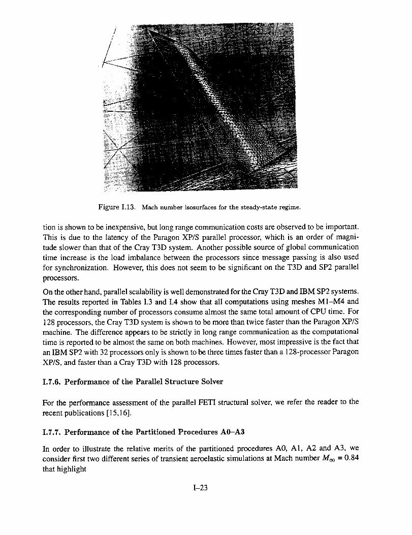
Figure 1.13. Mach number isosurfaces for the steady-state regime.

tion is shown to be inexpensive, but long range communication costs are observed to be important.

This is due to the latency of the Paragon XP/S parallel processor, which is an order of magni-

tude slower than that of the Cray T3D system. Another possible source of global communication

time increase is the load imbalance between the processors since message passing is also used

for synchronization. However, this does not seem to be significant on the T3D and SP2 parallel

processors.

On the other hand, parallel scalability is well demonstrated for the Cray T3D and IBM SP2 systems.

The results reported in Tables 1.3 and 1.4 show that all computations using meshes M1-M4 and

the corresponding number of processors consume almost the same total amount of CPU time. For

128 processors, the Cray T3D system is shown to be more than twice faster than the Paragon XP/S

machine. The difference appears to be strictly in long range communication as the computational

time is reported to be almost the same on both machines. However, most impressive is the fact that

an IBM SP2 with 32 processors only is shown to be three times faster than a 128-processor Paragon

XP/S, and faster than a Cray T3D with 128 processors.

1.7.6. Performance of the Parallel Structure Solver

For the performance assessment of the parallel FETI structural solver, we refer the reader to the

recent publications [15,16].

1.7.7. Performance of the Partitioned Procedures A0-A3

In order to illustrate the relative merits of the partitioned procedures A0, AI, A2 and A3, we

consider first two different series of transient aeroelastic simulations at Mach number Moo = 0.84

that highlight

1-23

Figure 1.14. Initial perturbation of the displacement field of the wing.

the relative accuracy of these coupled solution algorithms for a fixed subcycling factor nS/F.

the relative speed of these coupled solution algorithms for a fixed level of accuracy.

In all cases, mesh M2 is used for the flow computations, 32 processors of an iPSC-860 system are

allocated to the fluid solver,'and 4 processors of the same machine are assigned to the structural

code. Initially, a steady-state flow is computed around the wing at Moo = 0.84 (Figure 1.13), a

Mach number at which the wing described above is not supposed to flutter. Then, the aeroelastic

response of the coupled system is triggered by a displacement perturbation of the wing along its

first mode (Figure I. 14).

First, the subcycling factor is fixed to ns/p -- 10 then to ns/e = 30, and the lift is computed using

a time-step corresponding to the stability limit of the explicit flow solver in the absence of coupling

with the structure. The obtained results are depicted in Figure I. 15 and Figure I. 16 for the first half

cycle.

The superiority of the parallel fluid-subcycled A3 solution procedure is clearly demonstrated in

Figure I. 15 and Figure I. 16. For ns/r = I0, A3 is shown to be the closest to A0, which is supposed

to be the most accurate since it is sequential and non-subcycled. A1 and A2 have comparable

accuracies. However, both of these algorithms exhibit a significantly more important phase error

than A3, especially for ns/t: = 30.

Next, the relative speed of the partitioned solution procedures is assessed by comparing their CPU

time for a certain level of accuracy dictated by A0. For this problem, it turned out that in order to

meet the accuracy requirements of AO, the solution algorithms A1 and A2 can subcycle only up to

1-24

Z5 //_/ _"¢_\ ALG2 - 10 lu0cl_M/// \\_,.tLG3 - 10 m_/O_

j "X

10 .

-5

-10

-15

*_0 r I 1 r I I I ! 10,_|_ 0.0014 0.00148 0.001_ 0.00155 0.0016 0.0011S_ 0.0017 0.00175 0.0010

Wne

Figure 1.15. Lift history for the first half cycle, ns/F = 10

30 .... , ,

/fj._I_ At.G|.:30 m N

18

tO

0 .......

'\\ :.,.

-10 \

\• 15 I I I I I I I _ I0.00135 0.0014 0.00145 0.0015 0.00155 0.0018 0.00|65 0.0017 0,00175 0.0018 0.00185

"rime

Figure 1.16. Lift history for the first half cycle, ns/F = 30

nS/F = 5, while A3 can easily use a subcycling factor as large as nsly = 10. The performance

results measured on an iPSC-860 system are reported on Table 1.5 for the first 50 coupled time-steps.

In this table, ICWF and ICWS denote the inter-code communication timings measured respectively

in the fluid and structural kernels; these timings include idle and synchronization (wait) time when

the fluid and structural communications do not completely overlap. For programming reasons,

ICWS is monitored together with the evaluation of the pressure load.

1-25

Table1.5.Performanceresults for coupled FSI problem on the Intel iPSC-860

Fluid: 32 processors, Structure: 4 processors

Elapsed time for 50 fluid time-steps

Alg. Fluid Fluid Struc. ICWS ICWF Total

Solver Motion Solver CPU

A0 177.4 s. 71.2 s. 33.4 s. 219.0 s. 384.1 s. 632.7 s.

A1 180.0 s. 71.2 s. 16.9 s. 216.9 s. 89.3 s. 340.5 s.

A2 184.8 s. 71.2 s. 16.6 s. 114.0 s. 0.4 s. 256.4 s.

A3 176.1 s. 71.2 s. 10.4 s. 112.3 s. 0.4s. 247.7 s.

1.8. CONCLUSIONS

From the results reported in Table 1.5, the following observations can be made.

The fluid computations dominate the simulation time. This is partly because the structural

model is simple in this case, and a linear elastic behavior is assumed. However, by allocating

32 processors to the fluid kernel and 4 processors to the structure code, a reasonable loadbalance is shown to be achieved for A0.

During the first 50 fluid time-steps, the CPU time corresponding to the structural solver does

not decrease linearly with the subcycling factor ns/e because of the initial costs of the FETI

reorthogonalization procedure designed for the efficient iterative solution of implicit systems

with repeated right hand sides [ 16].

The effect of subcycling on intercube communication costs is clearly demonstrated. The

impact of this effect on the total CPU time is less important for A2 and A3 which feature

inter-field parallelism in addition to intra-field multiprocessing, than for A1 which features

intra-field parallelism only (note that A1 with nS/F = 1 is identical to A0), because the flow

solution time is dominating.

Algorithms A2 and A3 allow a certain amount of overlap between inter-field communications,

which reduces intercube communication and idle time on the fluid side to less than 0.001% of

the amount corresponding to A0.

1-26

The superiorityof A3 overA2 is not clearly demonstratedfor this problembecauseof thesimplicity of the structuralmodelandtheconsequentloadunbalancebetweenthe fluid andstructurecomputations.

Most importantly,the performanceresultsreportedin Table5 demonstratethat subcyclingandinter-fieldparallelismaredesirablefor aeroelasticsimulationsevenwhenthe flow computationsdominatethe structuralones,becausethesefeaturescansignificantlyreducethetotal simulationtimebyminimizingtheamountof inter-fieldcommunicationsandoverlappingthem.Forthesimpleproblemdescribedherein,theparallelfluid-subcycledA2 andA3 algorithmsaremorethantwicefasterthantheconventionalstaggeredprocedureA0.

Acknowledgments

ThisworkwassupportedbyNASALangleyunderGrant NAG-1536427,by NASALewisResearchCenter under Grant NAG3-1273,and by the National ScienceFoundationunder Grant ASC-9217394.

1-27

Appendix II

LB: A Program for Load-Balancing Multiblock Grids

Summary

This Appendix describes recent research towards load-balancing the execution of ENGIO on parallel

machines. ENG10 is a multiblock-multigrid code developed by Mark Stewart of NYMA Research

Inc. to perform axisymmetric aerodynamic analysis of complete turbofan engines taking into ac-

count combustion, compression and mixing effects through appropriate circumferential averaging.

The load-balancing process is based on an iterative strategy for subdividing and recombining the

original grid-blocks that discretize distinct portions of the computational domain. The research

work reported here was performed by U. Gumaste under the supervision of Prof. C. A. Felippa.

ILl. INTRODUCTION

II.l.1. Motivation

For efficient parallelization of multiblock-grid codes, the requirement of load balancing demands

that the grid be subdivided into subdomains of similar computational requirements, which are

assigned to individual processors. Load balancing is desirable in the sense that if the computational

load of one or more blocks substantially dominates that of others, processors given the latter must

wait until the former complete.

Such "computational bottlenecks" can negate the beneficial effect of parallelization. To give an

admittedly extreme example, suppose that the aerodynamic discretization uses up 32 blocks which

are assigned to 32 processors, and that one of them takes up 5 times longer to complete than the

average of the remaining blocks. Then 31 processors on the average will be idle 80% of the time.

Load balancing is not difficult to achieve for unstructured meshes arising with finite-element or

finite-volume discretizations. This is because in such cases one deals with element-level granularity,

which can be efficiently treated with well studied domain-decomposition techniques for unstructured

meshes. In essence such subdomains are formed by groups of connected elements, and elements

may be moved from one domain to another with few "strings attached" other than connectivity.

On the other hand for multiblock-grid discretizations the problem is more difficult and has not, to

the writers' knowledge, been investigated in any degree of generality within the context of load

balancing. The main difficulty is that blocks cannot be arbitrarily partitioned, for example cell by

cell, because discretization constraints enforcing grid topological regularity must be respected.

The following is an outline of the program LB developed at the University of Colorado to perform

load-balancing of the multiblock discretization used in the program ENGi0. This is a multiblock-

multigrid code developed by Mark Stewart of NYMA Research Inc. to perform axisymmetric

II-1

aerodynamic analysis of complete turbofan engines taking into account combustion, compression

and mixing effects through appropriate circumferential averaging [35].

II.1.2. Requirements and Constraints

Multiblock grids are used to discretize complex geometries. A multiblock grid divides the physical

subdomain into topologically rectangular blocks. The grid pertaining to each block is regular

(structured). For bladed jet engine geometries, this is achieved by a series of programs also written

by Mark Stewart, namely TOPOS, TF and MS [36,37], which function as preprocessors to ENG10.

Efficient parallelization requires the computational load to be (nearly) equal among all processors.

Usually, depending upon the geometry, the computational sizes of component blocks of a multiblock

discretization vary and mapping one to each processor would not naturally ensure load balance.

The LB program attempts to load balance a given multiblock grid so that the resulting subdivisions

of the grid are of similar computational cost.

For re-use of F.2tG10 to be possible for the parallel version, it is required that the resulting subdivisions

of the original multiblock grid be also regular grids or are collections of blocks, each of which contain

regular grids. This imposed the restriction that the number of final subdivisions desired be greater

than the number of blocks in the original grid. Thus for most cases, ideally, the number of blocks

in the original grid should be 10 to 20, because 32 to 128 processors are normally used in present

generation MPPs. LB works better when the number of available processor substantially exceeds

the original number of blocks.

II.1.3. Multiblock Grid and MS

MS is a program that, given the domain discretization and blade forces, loss and combustor heating

data, etc., interpolates the data onto the grid. This program was used as a basis for LB as it possesses

the data structures most amenable to the task of load balancing.

Blocks are arranged in a C programming language linked list. Each block possesses a set of

segments that are lines joining grid points. The number of segments in each direction (transverse

and lateral) determines the computational size of the block. Segments can be of different types

depending upon where they are located as follows :

1. False boundary segments. These are segments located at the interface between blocks. These

are called "false" boundaries as they are not actual physical boundaries in the grid but merely

lines across which data has to be exchanged between two adjacent blocks. Knowledge about

the false boundaries is essential to determine block connectivity.

2. Internal and solid boundary segments. These are segments located at the interface of combus-

tors, blades, etc. Knowledge about the internal and solid boundary segments helps determine

the location of blades, combustors and other engine components.

3. Far-fieM boundary segments. These are segments located at the far-field boundaries of the

domain and are useful in imposing boundary conditions.

II-2

C7" C7" _" i C7"t i ! i t t i

I

Ii

Figure II.l.Blockdivisionpriorto merger.

II.2. ALGORITHM

A very simple yet efficient algorithm based purely on the geometry of the multiblock grid and block

connectivity was adopted for this program.

The input file containing the grid gives information only about the coordinates of the grid points,

block dimensions component segments and boundary data. Hence the first task is to determine

the block connectivity. This is done by analysing the false boundary information and determining

blocks across opposite sides of the same false boundary segment. Once the interconnectivity

between blocks is established, the total number of cells in the grid is calculated and that divided

by the number of final subdivisions desired gives an estimate of the average number of cells per

subdivision.

Based on this average value, blocks are classified into "small" blocks and "large" blocks. Large

blocks are those whose size is greater than the average size determined above, whereas small blocks

have a size less than or equal to the average size.

Large blocks are then split into smaller blocks, each of which has a size approximately equal to the

average size. Smaller blocks are collected into groups so that the total size of each group is equal

to the average size. This has been found to give excellent load balance for small grids, grids in

which block sizes are compatible, and grids for unbladed configurations. For more complex grids

satisfactory results have been obtained.

11.3 IMPLEMENTATION

II.3.1 Maximum Block Merger

As firststep,blocks from the originalgridare merged as much as possibleto generated larger

blocks.This isdone so as to maximize processorusage.

Consider two blocks as illustratedin FigureH.I. Assurnc thatload-balancingconditionsrequire

11-3

i

i

Figure II.2. Block after merger.

that each of the blocks be split into four blocks, vertically. Vertical splitting of blocks proceeds

from right to left since blocks are stored in that manner. It is seen that sub-blocks 1.4 and 2.4 are

clearly much smaller than the other sub-blocks and assigning an individual processor to each of

them would be wasteful. Also, if the number of sub-blocks of each of the blocks is reduced to

three from four, each of the processors will become overloaded. Therefore, the best solution to

this problem is to first merge both the blocks and then split their combination to get a better load

balance as shown in Figure II.2.

In this case it is seen that not only is the total number of sub-blocks reduced by one (implying that

one less processor will be required) but also the load balancing is more effective since sub-block

sizes are more compatible.

Blocks cannot be merged arbitrarily but only in those cases when the resulting larger block will

have a regular grid. This is illustrated in Figure II.3. As can be seen in that figure, it is possible to

merge block 1 with block 2 as their merging will result in the formation of a larger block in which

the grid is regular. However, block 3 cannot be merged with either of block 1 or 2 as the resulting

block would not have a top[ologically regular structure.

II.3.2. Block Classification

Once blocks are merged to the maximum permissible extent, all of them are passed through a

classifying routine by which they are tagged as "small" or "large."

II.3.3. Splitting of "Large" Blocks

Those blocks classified as "large" blocks are split into smaller sub-blocks, each having a size as

close as possible to the desired average size.

Blocks are split horizontally or vertically depending upon their dimensions. Wider blocks are split

vertically and narrower blocks are split horizontally. Splitting of a block involves generation of

a false boundary across the sub-blocks and checking for the presence of blades and other engine

I1-4

tal_ I,omm*ry

n IA. ,1.

Figure II.3. Possible block mergers.

components which cannot be "cut". This is done to ensure continuity in these critical regions.

II.3.4 Re-merging and Grouping

Once all the "large" blocks are split, the second phase of the program begins in which the blocks are

re-merged or grouped for maximum processor efficiency. This is done mainly to take very small

blocks into consideration, which can be explained with the help of the Figure II.4.

In this situation, there is a cluster of "small" blocks with no "large" block nearby. The program

selects a number of such "small" blocks and groups them into a cluster. Grouping is different

from merging. Blocks are not merged to produce a single larger block but they are only meant to

reside on the same processor. Grouping requires knowing block interconnectivity and proceeds in

a recursive fashion. First, all "small" blocks adjacent to the present block are considered. Then, if

the total number of cells of all the blocks is less than the average size, blocks adjacent to the block's

adjacent blocks are examined. This goes on until a sufficient number of cells are obtained.

There is another case which arises after a "large" block has been split resulting in the generation of

smaller sub-blocks, each being approximately equal to the average in size. In this case, again, the

adjacent "small" blocks are merged into one of the children of the parent "large" block. Here, only

one such block grouping is permitted since it should be noted that the "child" blocks are very close

to the desired average size and the processor on which they reside should not be further loaded.

This case is illustrated in Figure II.5.

II-5

b

a d

- lI,Blocks a, b, c and d would be "clustered"

Figure II.4. Grouping of small blocks.

|imiam|m|ii

• 1

iiiimJimim

false boundary of parent "large block"

.................. 1.........

/ bi i i mm an m inl_ i g u i i i i II u |

Figure II.5. Grouping of small mad l_trge blocks.

1]--6

II.3.5 Some Practical Considerations

It has been observed after going through several test cases that the process of load-balancing for

complex multiblock grids is not always deterministic and hence user inputs may be required to

make the process more predictable. This input comprises the following parameters.

MAX_TOL This is the maximum tolerable value to which a processor can be loaded, expressed

in terms of the average size. Usually values between 0.95 and 1.2 give sufficiently

good results.

MIN_TOL This is the minimum tolerable value to which a processor can be loaded, expressed

in terms of the average size. Usually values between 0.6 and 0.9 give sufficiently

good results.

It should be noted that in most cases, the load balancing is independent of the above parameters.

These attain significance only in case of very complicated geometries.

11.4 EXAMPLES

II.4.1 A Single Rectangular Block

This is the case of a single rectangular block having a regular grid. On this grid, a perfect load

balance was obtained for an unbladed block, and satisfactory balance for a bladed block.

II.4.2 Two Adjacent Rectangular Blocks

The next test case considered two adjacent blocks, each of which contains a regular grids. Again,

for this simple case, a perfect load balance was obtained for two unbladed blocks.

II.4.3 Grid for General Electric Energy Efficient Engine (GE-EEE)

This test case pertains to the Energy Efficient Engine model developed by General Electric. This

model has been used extensively as computational-intensive tests for ENG10 [35]. The grid was

generated using ENGi0 preprocessors [36,37]. It contains 19 original blocks with approximately

115,000 grid points.

The initial load balance is only 15%, as the computational load is heavily dominated by the light-

blue block of Figure 11.6. This block contains a very fine grid because of the presence of a multistage

compressor. A load balancing factor of approximately 80% was finally obtained. Stages of the

load-balancing process carried out by LB for this fairly complex model are illustrated in color

Figures 11.6 through 1/.9.

11-7

1].5 CONCLUSIONS

A simple but effective algorithm for load-balancing discretizations consisting of multiple regular-

grid blocks has been developed. Preliminary results suggest that the algorithm yields satisfactory

results in the test cases considered here. These test cases have included a axisymmetric aerodynamic

model of the complete GE-EEE, which has over 105 grid points. A load balance of approximately

80% was achieved for this demanding case.

A worthwhile refinement of LB would be the inclusion of block weights that account for computa-

tional intensity due to the presence of effects such as compression or combustion in specific regions.

Such weights might be estimated from CPU measurements on sequential or vector machines, and

fed to LB to further improve the decomposition logic.

Acknowledgement

Mr. Udayan Gumaste, who designedand wrote LB, would liketo thank Dr. Mark Stewart forhis

support and assistanceduringthe development ofthisprogram. He alsoacknowledges productive

suggestionsfrom Prof.Farhat.

11-8

Figure II.6 : Initial Grid for GE-EEE ENGI0 Model( 19 blocks, Load Balance : 0. ! 475 t

Figure II.7 : (;rid for GE-EEE model after Maximum Merging ofAdjacent Blocks

t Load Balance : 0. I 1231

Figure II.8 : Grid for GE-EEE Model after Cutting Large BlocksI I.oad Balance : 0.6553_

Figure II.9 : Final Configuration of GE-EEE (;rid produced by LBi I_oad Balance : 0.7943_

REFERENCES

°

,

.

.

.

,

.

°

.

10.

11.

12.

13.

W. K. Anderson, J. L. Thomas and C .L. Rumsey, Extension and application of flux-vector

splitting to unsteady calculations on dynamic meshes, AIAA Paper No. 87-1152-CP, 1987.

E. Barszcz, Intercube communication on the iPSC/860, Scalable High Performance Comput-

ing Conference, Williamsburg, April 26-29, 1992.

J. T. Batina, Unsteady Euler airfoil solutions using unstructured dynamic meshes, AIAA

Paper No. 89-0115, AIAA 27th Aerospace Sciences Meeting, Reno, Nevada, January 9-12,1989.

T. Belytschko, P. Smolenski and W. K. Liu, Stability of multi-time step partitioned integra-tors for first-order finite element systems, Comput. Meths. Appl. Mech. Engrg., 49 (1985)

281-297.

M. Blair, M. H. Williams and T. A. Weisshaar, Time domain simulations of a flexible wing

in subsonic compressible flow, AIAA Paper No. 90-1153, AIAA 8th Applied Aerodynamics

Conference, Portland, Oregon, August 20-22, 1990.

C. J. Borland and D. P. Rizzetta, Nonlinear transonic flutter analysis, AIAA Journal, 20

(1982) 1606-1615.

J. Donea, An arbitrary Lagrangian-Eulerian finite element method for transient fluid-

structure interactions, Comput. Meths. Appl. Mech. Engrg., 33 (1982) 689-723.

C. Farhat and T. Y. Lin, Transient aeroelastic computations using multiple moving frames of

reference, AIAA Paper No. 90-3053, AIAA 8th Applied Aerodynamics Conference, Portland,

Oregon, August 20-22, 1990.

C. Farhat, K. C. Park and Y. D. Pelerin, An unconditionally stable staggered algorithm for

transient finite element analysis of coupled thermoelastic problems, Comput. Meths. Appl.

Mech. Engrg., 85 (1991) 349-365.

C. Farhat, S. Lanteri and L. Fezoui, Mixed finite volume/finite element massively parallel

computations: Euler flows, unstructured grids, and upwind approximations, in Unstructured

Scientific Computation on Scalable Multiprocessors, ed. by P. Mehrotra, J. Saltz, and R.

Voigt, MIT Press, (1992) 253-283.

C. Farhat and T. Y. Lin, A structure attached corotational fluid grid for transient aeroelastic

computations, AIAA Journal, 31 (1993) 597-599

C. Farhat, L. Fezoui, and S. Lanteri, Two-dimensional viscous flow computations on the

Connection Machine: unstructured meshes, upwind schemes, and massively parallel compu-

tations, Comput. Meths. Appl. Mech. Engrg., 102 (1993) 61-88.

C. Farhat and M. Lesoinne, Automatic partitioning of unstructured meshes for the parallel

solution of problems in computational mechanics, Internat. J. Numer. Meths. Engrg., 36,

(1993) 745-764.

R-1

14.

15.

16.

17.

18.

19.

20.

21.

22.

23.

24.

25.

C. FarhatandS.Lanteri,Simulationof compressibleviscousflowsonavarietyof MPPs:com-putational algorithmsfor unstructureddynamicmeshesand performanceresults,Comput.

Meths. Appl. Mech. Engrg., 119, (1994) 35-60.

C. Farhat, L. Crivelli and F. X. Roux, A transient FETI methodology for large-scale parallel

implicit computations in structural mechanics, Internat. J. Numer. Meths. Engrg., 37, (1994)1945-1975.

C. Farhat, L. Crivelli and F. X. Roux, Extending substructure based iterative solvers to

multiple load and repeated analyses, Comput. Meths. Appl. Mech. Engrg., 117 (1994) 195-209.

C. Farhat, S. Lanteri and H. D. Simon, TOP/DOMDEC, A software tool for mesh partition-

ing and parallel processing, J. Comput. Sys. Engrg., in press.

C. Farhat, P. S. Chen and P. Stern, Towards the ultimate iterative substructuring method:

combined numerical and parallel scalability, and multiple load cases, J. Comput. Sys. Engrg.,

in press.

A. Geist, A. Beguelin, J. Dongarra, R. Mancheck, V. Sunderam, PVM 3.0 User's Guide and

Reference Manual, Technical Report ORNL/TM-12187, Oak Ridge National Laboratory,1993.

G. P. Guruswamy, Time-accurate unsteady aerodynamic and aeroelastic calculations of wings

using Euler equations, AIAA Paper No. 88-2281, AIAA 29th Structures, Structural Dynamics

and Materials Conference, Williamsburg, Virginia, April, 18-20, 1988.

W. J. Hesse and N. V. S. Mumford, Jet Propulsion .for Aerospace Applications, 2nd ed.,

Pitnam Pubs., New York, N.Y., 1964, Chapter 11.

O. A. Kandil and H. A. Chuang, Unsteady vortex-dominated flows around maneuvering

wings over a wide range of mach numbers, AIAA Paper No. 88-0317,AIAA 26th Aerospace

Sciences Meeting, Reno, Nevada, January 11-14, 1988.

S. Lanteri and C. Farhat, Viscous flow computations on MPP systems: implementational

issues and performance results for unstructured grids, in Parallel Processing for Scientific

Computing, ed. by R. F. Sincovec et. al., SIAM (1993) 65-70.

M. Lesoinne and C. Farhat, Stability analysis of dynamic meshes for transient aeroelastic

computations, AIAA Paper No. 93-3325, 11th AIAA Computational Fluid Dynamics Con-

ference, Orlando, Florida, July 6-9, 1993.

M. Lesoinne and C. Farhat, Geometric conservation laws for aeroelastic computations Using

unstructured dynamic meshes, AIAA Paper No. 95-1709, 1995.

M. Loriot, MS3D: Mesh Splitter for 3D Applications, User's Manual.

N. Maman and C. Farhat, Matching fluid and structure meshes for aeroelastic computations:

a parallel approach, Computers _ Structures, in press.

R-2

28.

29.

30.

31.

32.

33.

34.

35.

36.

37.

38.

39.

40.

41.

B. NKonga and H. Guillard, Godunovtype methodon non-structuredmeshesfor three-dimensionalmovingboundaryproblems,Comput. Meths. Appl. Mech. Engrg., 113, (1994)183-204.

K. C. Park, C. A. Felippa and J. A. DeRuntz, Stabilization of staggered solution procedures

for fluid-dtructure interaction analysis, in Computational Methods for Fluid-Structure Inter-

action Problems, ed. by T. Belytschko and T. L. Geers, AMD Vol. 26, American Society of

Mechanical Engineers, ASME, New York (1977) 95-124

K. C. Park and C. A. Felippa, Partitioned analysis of coupled systems, in: Computational

Methods for Transient Analysis, T. Belytschko and T. J. R. Hughes, Eds., North-Holland

Pub. Co. (1983) 157-219.

S. Piperno and C. Farhat, Partitioned procedures for the transient solution of coupled aeroe-

lastic problems, Comput. Meths. Appl. Mech. Engrg., to appear.

E. Pramono and S. K. Weeratunga, Aeroelastic computations for wings through direct cou-

pling on distributed-memory MIMD parallel computers, AIAA Paper No. 94-0095, 32nd

Aerospace Sciences Meeting, Reno, January 10-13, 1994.

R. D. Rausch, J. T. Batina and T. Y. Yang, Euler flutter analysis of airfoils using unstruc-

tured dynamic meshes, AIAA Paper No. 89-13834, 30th Structures, Structural Dynamics and

Materials Conference, Mobile, Alabama, April 3-5, 1989.

V. Shankar and H. Ide, Aeroelastic computations of flexible configurations, Computers 8J

Structures, 30 (1988) 15-28.

M. L. Stewart, Axisymmetric aerodynamic numerical analysis of a turbofan engine, Draft

paper, NASA Lewis Research Center, May 1994.

M. L. Stewart, Description of ENG10 subroutines and related programs, NASA Lewis Re-

search Center, October 1994.

M. L. Stewart, A Multiblock Grid Generation Technique Applied to a Jet Engine Configu-

ration, NASA CP-3143, NASA Lewis Research Center, 1992.

T. W. Strganac and D. T. Mook, Numerical model of unsteady subsonic aeroelastic behavior,

AIAA Journal, 28 (1990) 903-909.

T. Tezduyar, M. Behr and J. Liou, A new strategy for finite element computations involving

moving boundaries and interfaces - The deforming spatial domain/space-time procedure: I.

The concept and the preliminary numerical tests, Comput. Meths. Appl. Mech. Engrg., 94

(1992) 339-351.

P. D. Thomas and C. K. Lombard, Geometric conservation law and its application to flow

computations on moving grids, AIAA Journal, 17, (1979) 1030-1037.

B. Van Leer, Towards the ultimate conservative difference scheme V: a second-order sequel

to Godunov's method, J. Comp. Phys., 32 (1979).

R-3