High Corruption Income in Ming and Qing China

Shawn NiUniversity of Missouri

Pham Hoang Van ∗

University of Missouri

February 2005

Abstract: We develop an economic model that explains historical data ongovernment corruption in Ming and Qing China. In our model, officials’extensive powers result in corrupt income matching land’s share in output.We estimate corrupt income to be between 14 to 22 times official incomeresulting in about 22% of agricultural output accruing to 0.4% of thepopulation. The results suggest that eliminating corruption through salaryreform was possible in early Ming but impossible by mid-Qing rule. Landreform may also be ineffective because officials could extract the same rentsregardless of ownership. High officials’ incomes and the resulting inequalitymay have also created distortions and barriers to change that could havecontributed to China’s stagnation over the five centuries 1400-1900s.

JEL Codes: O10, O53

Keywords: Corruption, China

∗Department of Economics, University of Missouri, Columbia MO 65203; nix@missouri.edu andpham@missouri.edu. We have benefited from comments by Emek Basker, Pinaki Bose, James Foster, HenryWan Jr., and participants in presentations at the U. of Colorado-Denver, the Missouri Economics Conferencein Columbia and the Western Economics Association Meetings in Denver. We would also like to thank theeditor and two anonymous referees for insightful comments and suggestions. All errors are, of course, ourown.

1 Introduction

Under the Ming dynasty (1368-1644), China’s tax revenues and government spending

declined significantly. Mokyr (1990) argued that cutbacks in spending under-funded the

production of industrial goods that previously had been sponsored by the Sung

(960-1279) government. In this paper, we argue that the same fiscal tightening during the

Ming lowered government officials’ salaries to a point that allowed corruption to take

root. Corruption became more entrenched through the Ming and the Qing dynasty

(1644-1911) and potential rents expanded with the country’s increase in land and labor

endowments. The result was significant growth in the official’s rent-seeking income

even when per-capita output stagnated. Our model estimates corrupt income to be 14 to

22 times official income circa 1873 resulting in about 22% of agricultural output accruing

to 0.4% of the population. By the time the Qing government attempted to curb

corruption by raising salaries, rent-seeking income was so high and corruption so

entrenched that a three-fold increase in salary could not—and as we will show, no

fiscally feasible increase could—restore honest behavior.1

This paper presents a model of corruption in the Chinese countryside that allows us

to quantify the high and expanding levels of corruption incomes under the Ming and

Qing. High corruption incomes for officials may be important because they coincided

with a period of Chinese decline. Historians consider China under the Sung and Tang

(618-907) dynasties to be the world technological leader during which innovations like

gun powder, iron casting, textile spinning, time measurement, water power, and

advanced cultivation techniques were found in China well before their introductions in

Europe (see Mokyr (1990)). Decline seems to have started with the Ming and continued

through the Qing and a divergence between Europe and China was apparent after the

1The effect of low salaries on corrupt behavior is a type of efficiency wage story for corruption deterencewhich has been discussed by previous authors (for example, see Van Rijckeghem and Weder (1997); Chandand Moene (1999); Mookherjee (1997)).

start of the Industrial Revolution.2 While we do not attempt to establish in this paper

that high corruption incomes caused this decline, the literature on corruption provides

many strong arguments linking high corruption incomes and poor economic

performance.3

In building the model, we make two key assumptions that are motivated by the

historical context, and allow us to obtain tractable results. First, we start from the idea

found in previous models of corruption (for example, Schleifer and Vishny (1993)) where

the official is seen as a monopolist selling a government service. But in Ming and Qing

China, the official had wide-ranging authority, at times serving simultaneously as

tax-collector, judge, and employer so that, in effect, the corrupt official was selling a

wide range of services. Within villages, transactions are usually not anonymous. Thus, a

corrupt official could price discriminate almost perfectly for each of the services he

provided and could extract maximum rents from the local farmers. For modeling

purposes, we approximate the situation as the corrupt official levying an “corruption

tax” on income.

Second, Park (1997) reported that the penal code dictated very harsh penalties for

corruption but did not increase much with the extent of the corrupt act. Therefore, if the

official found it in his interest to be corrupt at all, he would want to extort as much as

possible. And although penalties were harsh on paper, the evidence suggests

2We should note that not all historians agree that China fell behind Europe during this time. Pomeranz(2000), for instance, argued that around 1750, Europe and certain regions in China had similar industriesand economic performance. A critique of Pomeranz’s argument can be found in Brenner and Isett (2002).

3For instance, high incomes from rent-seeking draws talent away from productive activities (Murphy,Shleifer, and Vishny (1991)); rent-seeking subjected the rural population to an extremely high effective taxburden (45% by our estimates); high corruption incomes strengthened monopolies and created obstaclesto positive change (Parente and Prescott (2000), Acemoglu and Robinson (2002)); high incomes for officialsconcentrated wealth to the small gentry class (we estimate that around 1873, 0.4% of the population re-ceived 22% of agricultural output) and the extreme income inequality may have prevented the formationof demand for mass consumption of industrial goods (Murphy, Shleifer, and Vishny (1989)). We shouldalso note arguments that some corruption might be optimal (Acemoglu and Verdier (2002), Huntington(1968) and Leff (1964)). However, empirical evidence suggests that corruption causes lower investmentand growth (see Mauro (1995)).

2

punishment came down only on a small fraction of the number of corrupt officials so

that the expected value of punishment was not that high. Thus, many officials would

choose to be corrupt and his corrupt income would be determined by the optimal

“corruption tax” rate. The rate turns out to be land share’s of output. So by the power of

their positions, government officials were the de facto landlords in rural China, receiving

land’s share of output and accruing almost the entire agricultural surplus. We exploit

this result to calculate the corrupt official’s potential income at various periods.

We should note from the outset that we abstract away from many issues discussed

in the vast literature on corruption (see Bardhan (1997) for a survey). The reason for

doing so is not to deny the importance of such issues but rather, our approach is

motivated by the evidence on salaries and corruption in this particular period of

history.4 The fact that our simple model yields results that closely match estimates by

China historians says that it is a good first approximation useful as a tool to talk about

corruption in this period.

The next section presents historical evidence on low salaries and corruption in Ming

and Qing China. This serves as the motivation for the model of corruption presented in

section 3. In section 4, we calculate a range for potential corruption income as a ratio to

salary using parameters for the economy under the Qing. We use this benchmark

calculation to impute the level of rent-seeking during various points of Ming and Qing

rule. In section 5 we impute the salaries that would have had to be paid to induce

officials to be honest and argue that when punishment probabilities are state-dependent

this salary level was fiscally untenable under the Qing. Section 6 concludes.

4For example, we don’t consider the issues of monitoring and detection because the evidence suggeststhat during Ming and Qing times (and even in many countries today), corrupt officials are often easilyidentifiable but punishment came down only on a few and usually for reasons not associated with theactual corrupt act.

3

2 Historical Evidence Of Low Salary and High Corruption

“The Ming system represents a significant break in Chinese fiscal history.

From this time onwards the main aim of governmental finance was to

maintain the political status quo, and it ceased to exhibit dynamic qualities.”

Huang (1974, p. 323)

“... [C]orruption under the Ming was another result of inadequate

budgeting. The operating expenses of many offices were clearly below the

necessary minimum... Throughout the fifteenth century there were numerous

cases in the capital of officials heavily involved in corruption. ... In 1470

Minister of Personnel Yao Ku’ei reported that his office was haunted by

professional moneylenders ... offer[ing] selective loans to officials in the

capital ... The situation apparently worsened in the sixteenth century. The

recorded impeachment cases reveal a general lowering of moral standards.”

Huang (1974, p. 48)

Low government salaries may have allowed corruption to take root during the Ming

and to expand during the Ming and Qing. During the Ming era, tax revenues

plummeted and government official salaries were greatly reduced. The main source

(about 75%) of government revenue was the land tax. Throughout the three centuries of

Ming rule, grain collected as land tax showed little change. Total collection in 1502 was

about 27 million piculs (Huang (1974, p. 48)). Revenue under the Ming was considerably

lower than during the Sung dynasty when by the mid-eleventh century the annual state

budget had already reached 72 million copper cash units 5 (Lo (1987, Table 1)).

Consistent with low tax revenues, nominal pay for government officials was also

low. Fixed in 1392, the salary schedule effective throughout the Ming was not generous

at its inception and got increasingly meager as the real value of the payments

5One copper cash unit (or kuan) was approximately equivalent to one picul of grain (see Lo (1987)).

4

deteriorated over the next two centuries. By the fifteenth century, about half of salaries

were paid in grain, and half in commodities such as silk fabrics, cotton cloth, pepper and

sapanwood. By 1434, however, it was estimated that the value of the commodity

payments was only 4% of the scheduled amount. In 1432, some officials were paid with

confiscated garments and salvaged materials, and in 1472, peas were used as payment.

In the following year in Nanking, it was found that the peas “were suitable only for

feeding horses” (Huang (1974, p. 48)). From this account, it is apparent that salaries

steadily fell over the course of the Ming and by the mid-1400s, half of the salaries was

effectively unpaid!

The Qing rulers, being foreign conquerors (Manchu), tried to quickly restore

normalcy after taking power from the Ming. The new rulers thus avoided any major

institutional reforms particularly in the fiscal area (Huang (1974)). So salaries of the early

Qing officials were not much changed compared to the Ming. By contrast, the top Sung

officials were paid (excluding numerous regular allowances in kind) much higher

salaries than were paid to Ming and Qing officials. In 1012, nominal annual salaries for

Sung civil servants ranged from 96 kuan for low-level to 4,800 kuan for top-level officials

(Wong (1975)). This is considerably higher than Ming salaries in 1392 of 60 piculs of

grain for low-rank to 1,044 piculs for the top-rank officials (Huang (1974)). Comparing

the Sung to the Qing, Deng (1999, p. 302-3) reported that the “First Rank” Sung official

was paid about 10 times his Qing counterpart. Although this latter number may be too

high to be taken literally, it is clear that Sung officials were paid much higher than Ming

and Qing officials.

Government officials in 1773 England were also better paid than officials in Ming

and Qing China. We examined a document published by the Government of England

(1774) titled The True State of England listing the salaries of every officer, civil and

military, in all the public offices of Great Britain. Most English government officials

made several hundred pounds a year compared to £20 for watchmen and gardeners on

5

the government payroll. Salaries for top officials were much higher. For example, the

salary of the Secretary of State (including lawful perquisites) was £8,000; the High Court

of Chancery (top law official) made £2,100; the Receiver General (in charge of revenues

collected from customs in England and Scotland) made £1,000. To get an idea of how

this compares to the rest of the population at the time, family incomes in the “high”

category were above £150; the “middle class” between £30 and £150; and the “low”

income group below £30 (Jones (1988, Table 3.3)).

To be sure, England had its own problems with corruption. Up until the 1880s the

British civil service had to grapple with what was called “Old Corruption” where some

British officials were able to gain extra income by nominally serving in several posts at

once collecting multiple salaries and pensions (see Rubinstein (1983)). But since these

extra salaries were limited by statute, they were much smaller than that of most

corrupted Qing officials. In this sense, British “Old Corruption” was also more benign

than the corruption in ancient China. In England, extra income was derived from

sinecures, obtained through political favor. In Ming and Qing China, corruption income

was aggressively exacted from the private sector and therefore far more distortionary.

North and Weingast (1989) observed that the checks and balances established by the

Glorious Revolution in 1688 among the representative government, the court, and the

British Crown played a vital role in protecting property rights and setting the

precondition for industrial revolution.6 British “Old Corruption” did not affect property

rights the way corruption in ancient China did.

Just as high salaries were no guarantor against corruption, low salaries were, of

course, not sufficient cause for sustained large scale corruption either. What made the

officials in Ming and Qing China susceptible to the temptations of corruption is the

combination of low salary and the concentrated power of office. By the time of the Qing,

6We note a contrarian view by Clark (1996) who argued that the Glorious Revolution did not representa structural break because secure property rights in England existed even before 1688.

6

fee-taking and corruption made salary a negligible portion of income for an official

because there were ample opportunities to collect rents. Individual local government

officials served not only as administrators of public affairs but also as tax collectors and

judges of local courts. The multiple roles assumed by the individual officials made

checks on his power difficult.

This does not seem to have been the case in the Sung bureaucracy where even

though “officials were well paid, well treated, and on the whole well respected, ...

numerous checks and balances regulated the government operations. This was

particularly true in local government where administrators were placed under various

supervisory agencies as well as watched by the assistance under them.” (Liu (1962)).

Officials were rotated often, with each post lasting three or four years. The promotion of

an official required his superior’s sponsorship, an action involving a pledge of his

“entire being” to guarantee the integrity of the person being sponsored (see Lo (1987)

and Kracke (1953)). The result was very effective government which in Lo’s (1987)

words “set an unsurpassed standard.”

There is evidence of similar checks on power in the civil service system of

seventeenth-century England. During that time, when an English tax-payer disputed the

amount he was assessed to pay, he could file a legal challenge against the legality of the

tax or the conduct of the tax collector. Such challenges could not be ignored by the king.

Braddick (1996, pp.141-2) documented a tax-refusal case in 1636 in which Charles I had

to write a response to twelve common-law judges to justify the taxes he levied, with the

end result being a seven-to-five ruling for the king. The legal protection of tax-payers in

England appeared to be effective. Over the period 1558-1714, the only notable cases of

resistance were against the excise tax in 1640 and the hearth tax in the 1660s, both under

special circumstances (see Braddick (1996, pp. 170-4)). Though these examples refer to

the protection against unfair legal taxation, they do suggest a system of checks on power

that were not seen in Ming and Qing China.

7

Official salaries were raised significantly during the Qing in the hope of curbing

corruption. In the early Yung-cheng period (1727), allowances called yang-lien (honesty

nourishment) were instituted to supplement regular salaries. Key provincial and local

officials, as well as military officers, also received an additional allowance known as

kung-fei (administrative expenses). Chang (1962, p. 38) reported from Qing records that

the total legal annual income to all officials amounted to about 6.3 million taels of silver

including 1.4 million in salaries, 4.3 million yang-lien, and 0.6 million kung-fei. On

average, the extra allowance intended to curb corruption was over three times regular

salary.

It is not surprising that the salary reform had little impact on curbing corruption

because even though the salary increases were generous, compensation was still

negligible compared to incomes from corruption. The Ming and Qing economies were

much larger than the Sung economy. Increases in population (five-fold) and expansion

of cultivated land (three-fold) during the Ming and Qing increased the potential gain

from corruption, especially among the top rank of the government. Chang (1962)

estimated that around 1880, aggregate extra-legal income was about 115 million taels of

silver,7 shared among 23,000 Chinese officials, with more than half of the income shared

among 1,700 top officials. In other words, corrupt income was 18.5 times legal income!

This extraordinary amount came from office-holding alone and did not include the

officials’ income through land-holding and other activities in commerce, where they also

enjoyed advantages over common citizens.

7 Since extra-legal income was of course not recorded, Chang’s estimate cleverly made use of alternativeinformation. Clan records included assessment schedules of how much a clan member, depending on hisoffice title, was expected to contribute to the clan treasury. For instance, in the Huang clan, a ‘prefect’ andany rank above was expected to contribute twice as much as a ‘magistrate’ and a secretary or any rankbelow was expected to contribute one-fifth as much. These expected contributions Chang took to reflectincomes. Censor Hu Chia-Yu reported from his findings that a ‘magistrate’ made about 30,000 taels in extraincome. Taking this as a base, Chang applied the information from the clan assessment schedules to arriveat an estimate of extra income for each office. These he multiplied by the number of officials at each rankand aggregated to arrive at total extra-legal income.

8

The extra income from office-holding came at the expense of the small land-owning

farmers. For example, it was customary for a county magistrate to collect an extra

amount in proportion to the land tax quota set by the central government. Besides the

magistrates, provincial officials such as governors-general, governors, commissioners,

intendants, and prefects could also impose special fees. Other officials who did not

handle the flow of tax money received less extra income, mainly through cash presents

and gifts.

Given the widespread acts of gift-taking, acceptance of bribes, and extortion by

government officials, it is fair to assume that most corrupt officials went unpunished.

For those unlucky few, however, punishment, which was often affected by extralegal

factors, could be harsh and swift. Park (1997) cited the examples of Guizhou governor

Liangqing who was impeached in 1770 for accepting presents from a subordinate and

Zhejiang governor Fusong in 1793 who was impeached for soliciting fees to build an

excursion boat for his mother to travel to scenic locations. Though only a few thousand

taels were involved in each case, both men were executed. Their conduct, unremarkable

relative to that of other corrupted officials, brought them harsh punishment mainly

because they were under investigation for administrative failures, and their character

was viewed with suspicion by Emperor Qianlong. The law against corruption was

enforced in an arbitrary fashion because if it had been enforced according to the letter

nearly all officials would deserve capital punishment.

According to the punishment scale under Qing law, the penalties for very minor

offenses were quite stiff. For example, those who took up to 15 taels of silver in exchange

for unlawful favors were subject to 70 to 100 blows with “heavy bamboo” and those

caught taking over 80 taels would receive “death by strangulation” (Park (1997, Table

1)). The penalty of 70 to 100 blows of “heavy bamboo” for minor corruption would kill

most adults. Thus, the incremental penalties beyond that would not be so meaningful

for most small bribe-takers. Therefore, it is reasonable to say that should a corrupt

9

official be prosecuted, the penalty is fairly flat over a wide range of bribes. Thus, if an

official found it profitable to be corrupt at all, then he would extort as much as the

people were able to pay.8

In practice, penalties, though heavy-handed, were usually handed out arbitrarily,

and the probability that a corrupt official would be punished was quite small. During

the 60-year reign of Qianlong, there were only 400 reported cases of impeachment, and

most of these cases were never prosecuted (Ma (1974)). To assess the probability of being

penalized for corruption, consider that there were more than 20,000 ranked officials in a

given year, and assume that on average each official was in office for three years, then

there were over 400,000 officials during the Qianlong era (1736-1795). If all these officials

were corrupt to some degree, the probability of an official being impeached was then

about 0.001; the probability of further punishment was much smaller still.

The decline of China that began with the Ming dynasty begs the question: why did

the Ming rulers allow the budget to deteriorate and government salaries to fall to a point

that would trigger mass corruption? It is puzzling since the Ming arguably had much

more consolidated power than its predecessors. There is no definitive answer on why

the Ming rulers made the choices that they did. Here we only offer some possibilities.

First, under the Sung, predecessor to the Ming, China was constantly threatened by

foreign invaders and the presence of political competition kept corruption in check. By

contrast, the Ming and the Qing, up until their fall, were able to establish very effective

control over the country by a powerful government. Ironically, the elimination of outside

threats also meant less checks on power that made wholesale corruption possible.

The second reason may be mere ideological preference that prompted the fiscal

8One could argue that for an official prosecuted for grand-scale corruption, his own execution was buta small part of the punishment. The usual package of punishments also included execution of immediatefamily members and close relatives and the disgrace of family name. We could model this as infinite penaltybeing imposed when the extent of the corruption reached very high levels. Most officials would not havebeen able to extract rents on such a scale. Thus the penalty is effectively a flat function of corruption.

10

restructuring at the start of the Ming. The founding Ming emperor, Hung-wu, came

from humble roots (he was once a beggar) achieving power by leading peasants and

commoners to drive out the Mongol invaders. Upon gaining power, he directed an effort

to reduce tax collection to grant relief to farmers and reduced the size of the central

government. Administrative matters formerly under the purview of the central

government were delegated to provincial authorities (Lo (1987, p. 224)). The founding

emperor also saw no need for a cumbersome system of checks and balances. With the

benefit of hindsight, it appears that low taxes and smaller government need not in and

of themselves be growth-stimulating. Low taxes resulted in a lowly paid and

insufficiently monitored government bureaucracy, a formula for breeding corruption

and extremely high effective taxes on commoners as a consequence. Moderately higher

taxes may not necessarily stifle growth. In England, the tax share of national income was

mostly between 13% to 16% in the second-half of the 1700s and first-half of the 1800s,

reaching as high as 24% during war (Hartwell (1981, Table 2)).

Finally, corruption may exhibit hysteresis. The low government salaries that

accompanied the reduction in the government budget at the start of the Ming only

triggered corruption. Once the system was thoroughly corrupt, reform became virtually

impossible as we show below.

3 A Model Of Corruption In Ming And Qing China

Below, we present a model motivated by aspects of salaries and corruption in Ming and

Qing China highlighted in the previous section. This simple model will allow us to make

calculations that quantify the relationship between salaries and corruption income.

Interestingly, our calculation is about the same as an earlier estimate by Chang (1962)

using available information on the expenditures of officials. Our result will also help

explain some of the events in the Ming and Qing period.

11

The key elements of the model are the following. There is a given number of

government officials each having jurisdiction over an equal number of citizens. As

motivated above, the local official, because if his broad authority in the village, is a

monopolist able to price discriminate almost perfectly for each of the services he

provides. In effect, an official has the ability to levy a tax on income. Therefore, we

assume that a corrupt official imposes a “corruption tax” at a rate b on the farmer’s

after-[legal]-tax output.9

In pre-modern China, landownership was highly skewed. A large fraction of the

population was landless and had to work on someone else’s land for a wage or as

sharecroppers. This wage (or income as share tenant) was low and relatively constant

over the five centuries of Ming and Qing rule. Thus, this group did not really contribute

to the corrupt officials’ income or to the government tax base. The corrupt official’s extra

income came mainly from the portion of population that owned enough land to have

surplus. For our purposes, we need only model this group’s behavior. Represent the

number of farmers falling into this sub-population as βN and the amount of land that

they owned as γT where N and T are the aggregate population and cultivated land area

respectively, β is the fraction of population in this group and γ is the fraction of land that

they owned.

These βN “small” farmers each supply effort, l ∈ [0, 1], on his own plot. The

opportunity cost of his effort is the market wage, w, which he takes as given. Production

takes the form Y = g(T , l) = A(γT)1−α(βNl)α, where α is labor’s share of output and A

is a productivity parameter. 10 To save notation, henceforth we write the production

9Though this is a static model, it captures the theme of the dynamic issue discussed by Olson (2000)of the trade-off between taking a big piece of slow-growing output and a smaller piece of faster-growingoutput.

10Historical evidence suggests that wages changed little over the five centuries we consider. Grain con-sumption per capita varied narrowly between 250 and 300 kilograms over this period (Perkins (1969, pp.14-7, Appendix F)). We refrain from calling this a subsistence wage since as Perkins pointed out, this levelof grain consumption was quite high by world standards at around 1957. The constancy of output percapita implies that grain yields changed over time as the land-to-labor ratio changed. Between 1400 and

12

function as g(l).

A fraction of output is turned over to the emperor in taxes. The corrupt official

extracts a fraction, b, of after-tax output. We assume that both farmers and officials are

risk-neutral and that all farmers and officials are identical. The representative small

farmer’s problem can be written as follows,

maxl

{(1 − b)(1 − t)A(γT)1−α(βNl)α − wβNl}.

A note on the form of the tax function is in order. About 75% of tax revenues during the

Ming took the form of a land tax. The share declined under the Qing but was still the

primary source of revenue, making up 43% of total revenues in 1908. For the farmers,

the land tax was the main form of taxation. These taxes were assessed on the land and

quotas were set for each district. Thus, the form of the land tax was neither lump-sum

nor ad valorem. Since the tax was assessed on the land, and if the assessment was an

accurate reflection of the quality as well as size of the plots, then total collection should

in principle be proportional to output. But from the farmer’s point of view, having

already owned a fixed plot of land, he is only expected to turn over a fixed quota as land

tax regardless of how much he actually produces.

It turns out that the specific way the tax is assessed is not important in this model.

The model we build here is for the purposes of calculating the fraction of after-tax

output that goes to the corrupt officials, b. Thus, we are only interested in the amount of

after-tax output and not the specific form of the tax that yields it. It is useful then to think

of t merely as the fraction of output that is turned over as tax with no connotation of how

it is assessed. The advantage of expressing the tax as a fraction of output is that it allows

1913, population increased five-fold and cultivated land three-fold. In order for output per capita to remainconstant, productivity, A, must have risen by (5/3)0.4 −1 (assuming α = 0.6) or 23% over 500 years — an av-erage annual growth of 0.04%. Though the annual gains were modest, the cumulative effect was not trivial.Perkins attributed the rise in grain yields to marginal changes in cropping patterns, the use of hydraulics,and increasing use of organic and chemical fertilizer.

13

us to apply the model to data for calculations. This will be apparent in the next section.

Work effort, l, satisfies the marginal condition

βNl = γT

(α(1 − b)(1 − t)A

w

) 11−α

. (1)

A fraction of tax revenue is used to pay officials’ salaries. The remaining fraction

goes to the government treasury which is spent on such things as the military,

infrastructure, and the royal court’s consumption. For the sake of simplicity, we assume

that this part of tax receipts is simply disposed of.

In addition to his salary, S, the corrupt official collects rents with a chance, q, that he

will be discovered and punished.11 If caught and punished, the penalty imposed on him,

D(B), would depend on the total amount he has extorted, B = b(1 − t)g(l).12 The

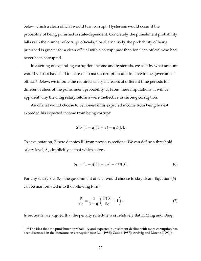
penalty function, D(B), has the following properties. D is zero for B = 0, but jumps

discontinuously as B increases from zero. Thus if he is caught collecting even a small

bribe, his penalty would be D0 > 0. For B > 0, D is convex in B (see Figure 1). The

discontinuity of the penalty schedule D(B) at B = 0 and the flatness of the D(B)

schedule up to some level are motivated by the historical evidence on punishment noted

in the previous section.

The official’s expected utility, V , can be written as

V(B(b)) =

S, b = 0

(1 − q) (B(b) + S) − qD(B(b)), b > 0,(2)

where B(b) ≡ B(l(b)) and l(b) is the small farmer’s effort function given in equation (1).

11It has generally been documented that these corrupt officials often live lavishly, beyond what a gov-ernment salary could afford. Therefore, it is best to think of q not as the probability of the official’s corruptactions being detected but as the probability that he will be caught and actually punished.

12Alternatively, we can think of D(B) as the bribe that the corrupt official would have to pay to anothercorrupt official if he is caught (see Basu, Bhattacharya, and Mishra (1992)).

14

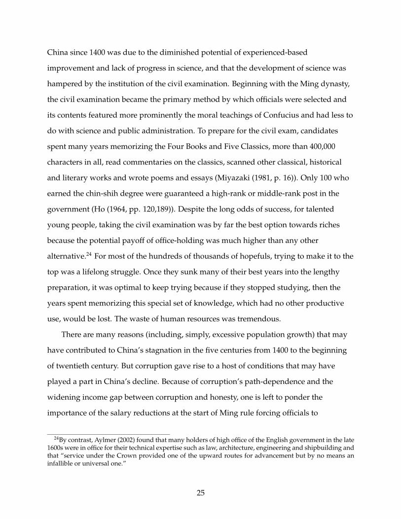
The official’s problem is maxb>0 V(b). An interior solution, b∗ satisfies the first-order

condition

B ′(b) ((1 − q) − qD ′(B(b))) = 0,

which results when either

B ′(b∗) = 0, or (3)

(1 − q) − qD ′(B(b∗)) = 0. (4)

To understand the intuition of this solution, b∗, we can think of the official’s problem

the following way. First, the official chooses a B∗ that would maximize expected utility.

Then, he would select a b∗ to achieve this optimal B∗ = B(b∗). This is illustrated in

Figure 2. In the top panel, the optimal B∗ is shown as the value which solves equation

(4), and the bottom panel shows the optimal choice of b∗ solving B∗ = B(b∗). Consider

the lower of the two values of b∗ that solves B∗ = B(b∗).

As drawn in Figure 2, the optimal choice of B∗ exceeds Bmax = max B(b), or in other

words, the B∗ that solves (4) is not achievable by any choice of b∗. The official would

have to settle for B∗ = Bmax which solves equation (3). The flatness of the D(B) schedule

that the historical record suggests makes the B∗ solving (4) unreachable. The intuition of

the flat D(B) schedule is now apparent. Since the penalty is in effect almost equally harsh

for any degree of corruption, if an official is corrupt, he will try to extract as much as he

can from the worker without regard for the additional penalty that it would bring.13

Substituting the worker’s effort function (1) into (3) and simplifying gives

(1 − b)α

1−α

[1 −

b

1 − b

α

1 − α

]= 0, or

b = 1 − α.

13The model setup is in the spirit of Becker’s (1968) model of crime and corruption, though our applica-tion to pre-modern China makes this more of an optimal taxation problem.

15

This result is not surprising. Government officials get land’s share of output. By

holding wide-ranging authority over people in their respective locales, government

officials are in effect the de facto landlords in the economy. The income of office-holders

from corrupt activity would be a fraction (1 − α)(1 − t) of the small landowners’ output.

The effective tax burden on the small farmer is (1 − α) + αt.

4 A Numerical Exercise

4.1 Corruption Income Around 1873

In this section, we use the results of the model to calculate the ratio of income from

corrupt activity to the officials’ salaries using parameters from the Qing period around

1873. This ratio is given by:

B

S=

(1 − α)(1 − t)A(γT)1−α(βNl)α

mStotal

,

where m is the fraction of total salaries that went to officials in the countryside and

Stotal is total salaries going to all officials in China. The numerator, corruption income,

is calculated as the share of after-tax output that goes to the corrupt officials derived in

the previous section. The denominator gives the total government salaries of officials in

the countryside.

First start with the denominator. For m, the fraction of total salaries going to officials

in the countryside, we take the share of agriculture output in total GNP which, in 1880,

Chang (1962, Table 40) estimated to be 60%.14 Around 1880, salaries of all government

officials in China were about 8% of land tax revenues.15 Thus we can write

14Qing records include production figures in the 1880s for major sectors in the economy, including agri-culture, which can be aggregated to get GNP. Alternatively, we could have taken m = 57% to be the numberof local and provincial officials as a fraction of the total number in China.

15This rate is the total salaries divided by total land tax revenue. Total salaries were reported by Chang

16

Stotal = 0.08rYag where Yag is agriculture output and r is total land tax revenue as a

fraction of grain output. For the value of r, we note land tax revenues were between

5.0% and 7.5% of grain output throughout the Qing years and between 8.9% and 2.5% at

various points during Ming rule.16

Recall that the parameter β is the fraction of the non-gentry population that owned

enough land to produce beyond subsistence (the small farmers) and γ is the fraction of

land that they owned. To estimate these parameters, we take the fraction of the

non-gentry population that owned more than 15 mou (about 2.5 acres) of land. These

farmers were thought to have surplus. Farmers with holdings between 3 and 15 mou

were at self-sufficiency while those with less than 3 mou of land had to find additional

work to survive17 (Chao (1986, p. 117)). Based on the limited records that existed,

previous studies suggest that land distribution in China did not change much

throughout the Sung, Ming and Qing (Chao (1986), and Brandt and Sands (1992)).

Therefore, we estimate these two parameters by averaging the values based on records

of five administrative districts at various periods.18 By this method, we get 28.3% for γ

and 20.3% for β.19

(1962, p. 38) from Qing records. Wang (1973) provided a detailed study of the land tax in Qing China. Hereported total land tax revenue for 1753 and for 1908. We interpolate from these two numbers to get landtax revenue for 1880.

16These fractions were calculated from records of land tax revenues divided by total grain output. Re-ceipts from the land tax during most of the Ming period was between 26 and 28 million piculs of grain aftera high of 34 million in 1412. Receipts during the Qing years were estimated using the method describedin the previous footnote. For total grain output in the various years, we use the estimates of Perkins (1969,p. 17) derived from multiplying population by output per capita which he reasoned to be constant at 5.7piculs per head. The ranges on these tax rates reflect the ranges on estimates of population figures.

17We should note that land varied greatly in quality, but it is likely that the big landowners also got thebest land due to their influence in society. And so those who owned little land were also those who got thelower quality land.

18The records are for four villages: Ch’ang-chou in 1676, Hsiu-ning in 1711, Hsui-ning in 1716, Ch’i-menin 1850, and subdivisions of Chu-lu, Hopei in 1706, as reported in Chao (1986, Tables 6.4 and 6.5).

19Assuming the same labor-to-land ratio for all plots of land would mean that an additional 8% of thepopulation (of those who don’t have enough land of their own) would be working for a wage on the landowned by others. Some of these laborers could be working on the plots of small farmers. However, it islikely that most worked on gentry-owned plots since the size of the plots belonging to small farmers wereindeed small. Nonetheless, including this extra labor input into the production of small farmers wouldslightly increase the estimate of corruption income.

17

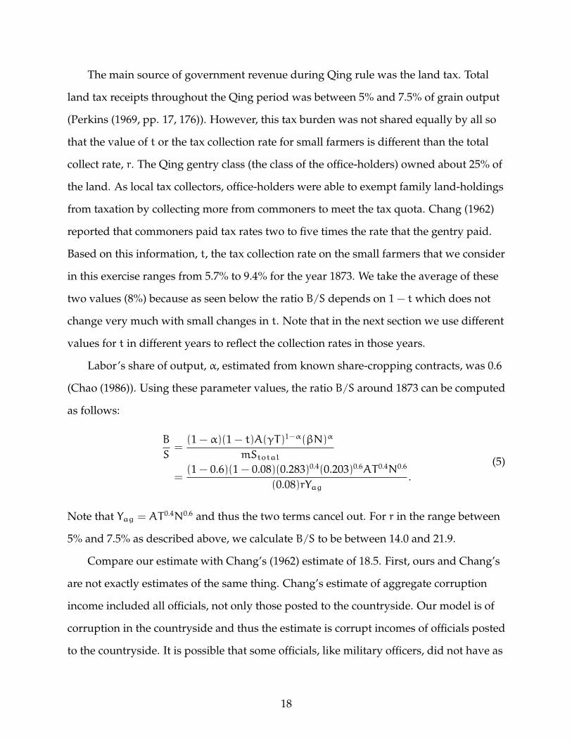
The main source of government revenue during Qing rule was the land tax. Total

land tax receipts throughout the Qing period was between 5% and 7.5% of grain output

(Perkins (1969, pp. 17, 176)). However, this tax burden was not shared equally by all so

that the value of t or the tax collection rate for small farmers is different than the total

collect rate, r. The Qing gentry class (the class of the office-holders) owned about 25% of

the land. As local tax collectors, office-holders were able to exempt family land-holdings

from taxation by collecting more from commoners to meet the tax quota. Chang (1962)

reported that commoners paid tax rates two to five times the rate that the gentry paid.

Based on this information, t, the tax collection rate on the small farmers that we consider

in this exercise ranges from 5.7% to 9.4% for the year 1873. We take the average of these

two values (8%) because as seen below the ratio B/S depends on 1 − t which does not

change very much with small changes in t. Note that in the next section we use different

values for t in different years to reflect the collection rates in those years.

Labor’s share of output, α, estimated from known share-cropping contracts, was 0.6

(Chao (1986)). Using these parameter values, the ratio B/S around 1873 can be computed

as follows:

B

S=

(1 − α)(1 − t)A(γT)1−α(βN)α

mStotal

=(1 − 0.6)(1 − 0.08)(0.283)0.4(0.203)0.6AT 0.4N0.6

(0.08)rYag

.(5)

Note that Yag = AT 0.4N0.6 and thus the two terms cancel out. For r in the range between

5% and 7.5% as described above, we calculate B/S to be between 14.0 and 21.9.

Compare our estimate with Chang’s (1962) estimate of 18.5. First, ours and Chang’s

are not exactly estimates of the same thing. Chang’s estimate of aggregate corruption

income included all officials, not only those posted to the countryside. Our model is of

corruption in the countryside and thus the estimate is corrupt incomes of officials posted

to the countryside. It is possible that some officials, like military officers, did not have as

18

many opportunities to extract extra income as those in the villages as their power is

confined to fewer activities. If Chang were to only look at the number of officials in the

countryside, his estimate would be closer to the higher end of our estimate.

Second, note, again, that Chang’s estimate comes from a rough examination of

expenditures (see footnote 7) while our estimate comes from a model of production and

corruption. That two different methodologies yield estimates that roughly agree lends

support to Chang’s estimate just as Chang’s estimate lends support to ours.

Finally, we should note that our simple model is one for potential corrupt income,

that is, the maximum rents that corrupt officials might be able to collect. It is possible

that not all officials were corrupt or that some of the corrupt ones, perhaps because of

dynamic considerations or institutional concerns not modeled here, opted not to extract

the highest possible rents. Interestingly, the fact that our calculations—of the maximum

rents possible—are close to Chang’s estimate using expenditure information means that

the Qing officials may have been pretty close to extorting all that they possibly could.

The gentry class also gained income from owning 25% of the land in China. Adding

this source of income to office-holding income brings the gentry’s total share of

agricultural output to

B + S + (Land Income)

Yag

= b(1 − t)(γ)1−α(β)α + mr + 0.25(1 − α)

which is between 21.5% and 23.0% (or an average of about 22%). We should note that

these numbers don’t include income derived from mercantile and other service activities

that the gentry were engaged in at the time. The model shows that the effective tax

burden on small farmers was (1 − α) + αt or about 45%.

19

4.2 The Evolution Of Corruption From Ming To Qing

Our model suggests that the official’s corruption income increased as population and

cultivated land increased.20 In this section, we calculate the ratio of corrupt income to

salary throughout the Ming and Qing using population and land estimates from past

researchers and salary levels inferred from the historical record.

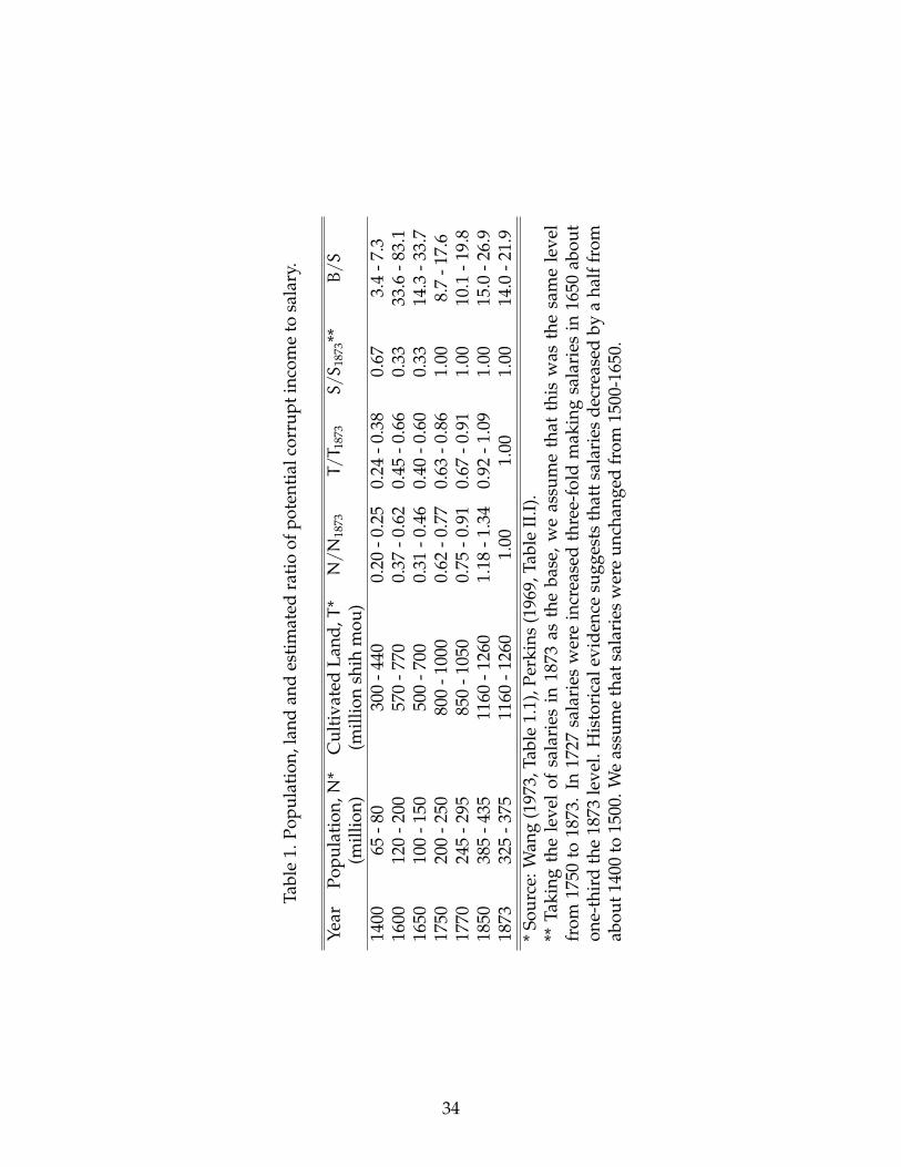
Table 1 shows that population increased almost five-fold from 1400 to 1913 while

land increased over three-fold over the same period. As noted in section 2, salaries were

reduced to very meager levels at the start of Ming rule and continued to fall in real terms

throughout the Ming. Salaries, by the mid-1400’s, were half the value at the end of the

1300’s, and were stagnant through the early Qing. In 1727, salaries were raised over

three-fold in an effort to curb corruption.

Wages were also stagnant throughout this period. We take these values to be

constant at the level in 1873. As was done in the previous section, we take the range of

values for the land tax collection rate found in the literature. From this, we calculate a

high and low values for the ratio B/S at various periods (reported in the last column of

Table 1) to get an idea of the evolution of corruption during the Ming and Qing. The

range of B/S is determined by the range of estimates for land and population in various

years as well as of the possible range on r, land tax revenues as a fraction of grain output.

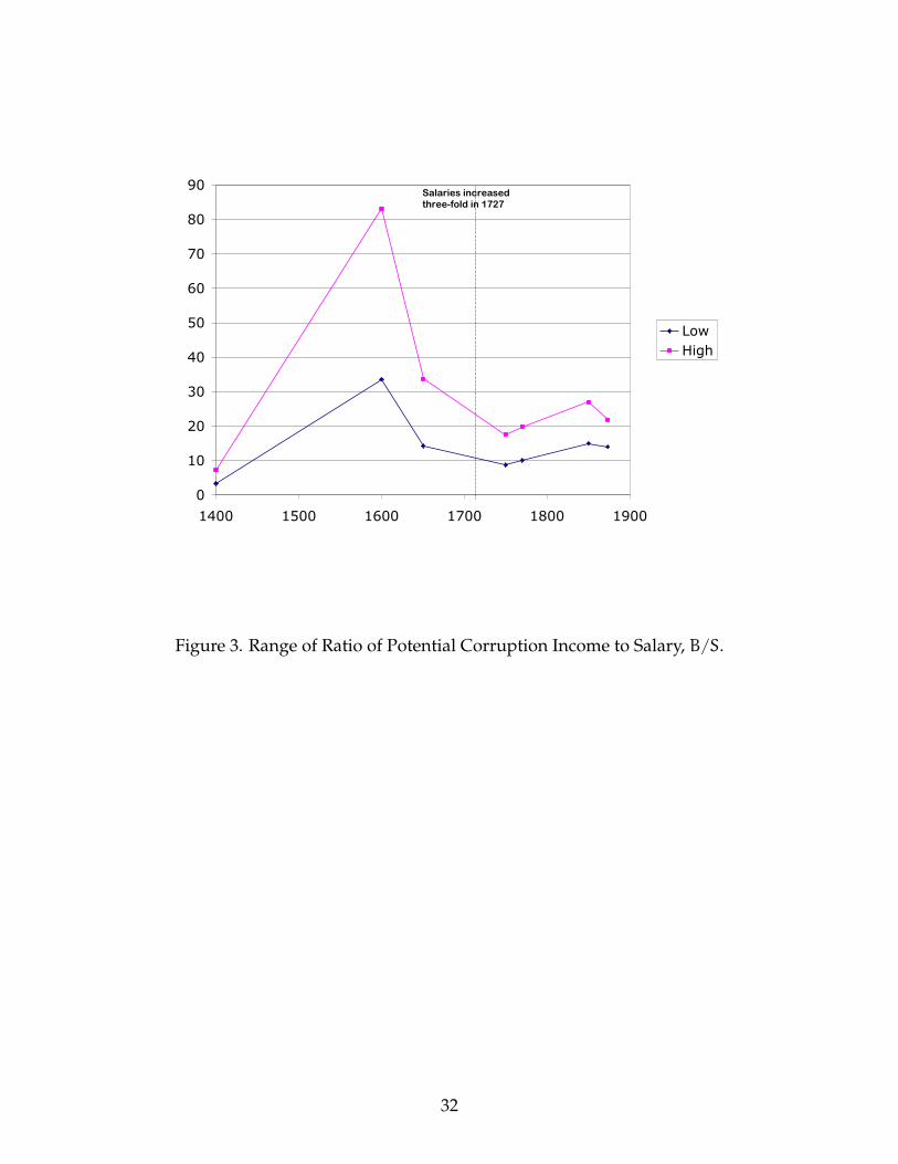
The plot of B/S is shown in Figure 3. In 1400, near the beginning of Ming rule, the

midpoint of the range of values for B/S was about 5.4. By 1600, the midpoint of the

range increased to about 58.4 as salaries fell to half the level in 1400 and output increased

from the expanding population and cultivated land.21 We should note that these values

20Although applied to a different context, Ades and Di Tella (2002) also suggested and documented thepositive relationship between the opportunity for rents and the level of corruption.

21The range of possible values in 1600 is large due to wide range of population estimates: 120-200 million.Note also that the range of values in 1873 is smaller than those in other years. This is because the value in1873 is used as a base and the values B/S in each year depends on the ratios N/N1873 and T/T1873. Thus foryears other than 1873, the ranges in possible values for N and T create a range of possible values for theratios N/N1873 and T/T1873.

20

are of the potential corruption incomes that could extracted. As we noted above, the

value for B/S we calculate for around 1873 is close to the estimate of Chang using

expenditure information. This implies that by 1873, officials might have actually been

close to extracting all they could. The historical evidence seems to indicate that

corruption got progressively worse through the Ming and Qing. And so the actual

corruption income during the Ming may much lower than potential corruption income

with the two quantities converging as time passed.

The drop in potential corruption income from 1600 to 1650 was because of drops in

population and cultivated land due to uprisings and armed resistance against the

Manchus at the end of the Ming era (see Wang (1973)). The drop from 1850 to 1873 was a

result of reductions in population also due to popular uprisings. After the salary reform

in 1727, the midpoint value in the range of B/S dropped to 13.2 in 1750. Compared to the

midpoint value of 24.0 in 1650, this was a significant decrease. However, income from

corruption was still so high relative to salary that the reform likely had little effect on

officials’ behaviors. We discuss this in more detail in the next section.

5 The Failed Salary Reform Under The Qing: Expanding

Corruption Income And Hysteresis

At the beginning of the Ming dynasty, government salaries took a significant drop.

Salaries may have dipped so low that corruption began to spread. During the Qing,

raising the salaries of officials failed to reduce corruption. There may be two factors why

the salary reforms were ineffective. First, as population and land expanded, output

increased and the potential income from corruption also increased making even the

higher salaries negligible in comparison. Second, hysteresis effects may have been

important. That is, even if income from corruption stayed constant, the threshold salary

above which a corrupt official would turn clean was far more than the threshold salary

21

below which a clean official would turn corrupt. Hysteresis would occur if the

probablity of being punished is state-dependent. Concretely, the punishment probability

falls with the number of corrupt officials,22 or alternatively, the probability of being

punished is greater for a clean official with a corrupt past than for clean official who had

never been corrupted.

In a setting of expanding corruption income and hysteresis, we ask: by what amount

would salaries have had to increase to make corruption unattractive to the government

official? Below, we impute the required salary increases at different time periods for

different values of the punishment probability, q. From these imputations, it will be

apparent why the Qing salary reforms were ineffective in curbing corruption.

An official would choose to be honest if his expected income from being honest

exceeded his expected income from being corrupt:

S > (1 − q)(B + S) − qD(B).

To save notation, B here denotes B∗ from previous sections. We can define a threshold

salary level, SC, implicitly as that which solves

SC = (1 − q)(B + SC) − qD(B). (6)

For any salary S > SC , the government official would choose to stay clean. Equation (6)

can be manipulated into the following form:

B

SC

=q

1 − q

(D(B)

SC

+ 1)

. (7)

In section 2, we argued that the penalty schedule was relatively flat in Ming and Qing

22The idea that the punishment probability and expected punishment decline with more corruption hasbeen discussed in the literature on corruption (see Lui (1986); Cadot (1987); Andvig and Moene (1990)).

22

China. For simplicity, then, let us assume a constant penalty, D(B) = D0, for all values of

B > 0. We take this value of D0 to be 50 times (this threshold) salary—twice the present

value of salary collected for 25 years at no discounting—to capture both lost income and

non-material loss. The required increase in salary is the ratio of the B/S ratio calculated

in the previous section to the ratio B/SC given in equation (7). A plot of the ratio of

required salaries (using the midpoint values of the ranges of B/S calculated in the

previous section and shown in Table 1) to have zero corruption to the estimated actual

salaries at various years for different values of q is shown in Figure 4.

Figure 4 shows a plot of SC/S over time taking the midpoint value of B/S of the

range calculated in the previous section. The required salary increase increased with

time as the potential corruption income rose and as actual salary fell throughout the

early Ming. In 1400, at the beginning of the Ming, for q = 0.1, salaries were right around

the threshold where an official would start finding it attractive to be corrupt. Salaries

during the Ming actually fell over the subsequent two centuries; corruption got worse.

Consider now the case for q = 0.001, a much lower probability of punishment. In 1750,

after the first set of Qing salary reforms, it would have taken an over 250-fold increase in

salary to bring about honesty—an amount exceeding all of agricultural output! In other

words, no possible level of salary would have been enough to “nourish honesty” as the

salary increase in 1727 had literally intended.

There are reasons to believe that when a system is corrupt, the probability of being

punished is much less, say q = 0.001,23 than the probability of being punished in a

system that is not corrupt, say q = 0.1. It is plausible to assume that the value of q at the

beginning of the Ming, when corruption just started to take root, was much greater than

the value of q during the Qing, when corruption was rampant. Thus, in Figure 4, the

plot for q = 0.1 is probably more applicable to the early Ming period and the q = 0.001

23The value q = 0.001 is consistent with the record of prosecutions from the 60-year reign of Qianlongduring the 1700s as discussed in section 2.

23

plot more applicable to the later Ming and the Qing period. What this shows then is that

had the early Ming emperors only kept salaries a little higher it would only have had to

let salaries grow with output to keep corruption in check. Had it kept that path, in 1750,

salaries would only have had to be about 2.3 times what it was to keep officials honest.

But because corruption was already well entrenched by that time, no salary increase

would have sufficed to restore integrity to the system. Another perspective on this

would be that the three-fold salary increase in 1727 might have been successful at

eradicating corruption if it had been accompanied by a purging of the incumbent

officials and replacing them with a completely new cadre of clean civil servants along

with an overhaul in the monitoring system (i.e., raising S and also raising q).

6 Concluding Remarks

The fortune of the Chinese official was tied directly to the land. The evidence supports

the implication of our simple model that the official’s income was the same as if he were

the landowner. Not surprisingly, uprisings to bring about land redistribution

throughout Chinese history did not have any lasting improvement in the standard of

living for farmers. Our model suggests that as long as officials possessed as much power

as they did in the countryside, nominal landownership did not matter since the corrupt

official could always extract land’s share of output by virtue of his position.

The model also suggests a close link between corruption and income inequality.

Murphy, Shleifer, and Vishny (1989) argued that extreme income inequality may prevent

industrialization from taking place because the absence of a middle class would mean

low demand for industrial goods. In pre-modern China, this might have been the case

with the root-cause being corruption. We should note again that inequality in

landholdings makes no real difference in this context.

Baumol (1990) and Lin (1995) suggested that the lack of technological progress in

24

China since 1400 was due to the diminished potential of experienced-based

improvement and lack of progress in science, and that the development of science was

hampered by the institution of the civil examination. Beginning with the Ming dynasty,

the civil examination became the primary method by which officials were selected and

its contents featured more prominently the moral teachings of Confucius and had less to

do with science and public administration. To prepare for the civil exam, candidates

spent many years memorizing the Four Books and Five Classics, more than 400,000

characters in all, read commentaries on the classics, scanned other classical, historical

and literary works and wrote poems and essays (Miyazaki (1981, p. 16)). Only 100 who

earned the chin-shih degree were guaranteed a high-rank or middle-rank post in the

government (Ho (1964, pp. 120,189)). Despite the long odds of success, for talented

young people, taking the civil examination was by far the best option towards riches

because the potential payoff of office-holding was much higher than any other

alternative.24 For most of the hundreds of thousands of hopefuls, trying to make it to the

top was a lifelong struggle. Once they sunk many of their best years into the lengthy

preparation, it was optimal to keep trying because if they stopped studying, then the

years spent memorizing this special set of knowledge, which had no other productive

use, would be lost. The waste of human resources was tremendous.

There are many reasons (including, simply, excessive population growth) that may

have contributed to China’s stagnation in the five centuries from 1400 to the beginning

of twentieth century. But corruption gave rise to a host of conditions that may have

played a part in China’s decline. Because of corruption’s path-dependence and the

widening income gap between corruption and honesty, one is left to ponder the

importance of the salary reductions at the start of Ming rule forcing officials to

24By contrast, Aylmer (2002) found that many holders of high office of the English government in the late1600s were in office for their technical expertise such as law, architecture, engineering and shipbuilding andthat “service under the Crown provided one of the upward routes for advancement but by no means aninfallible or universal one.”

25

supplement their meager incomes. Once the system was corrupted and the

opportunities for rents expanded, reforming the system became impossible. So while no

great historical trend can be explained without a multitude of events converging

together, it is at least fair to say that the policies at the beginning of the Ming contributed

to China’s sorry fate in the centuries subsequent.

References

Acemoglu, D., and J. A. Robinson (2002) “Economic Backwardness in PoliticalPerspective,” mimeo, U. C. Berkeley.

Acemoglu, D., and T. Verdier (2002) “Property Rights, Corruption and the Allocation ofTalent: a General Equilibrium Approach,” Economic Journal, 108(450), 1381–1403.

Ades, A., and R. Di Tella (2002) “Rents, Competition, Corruption,” American EconomicReview, 89(4), 982–93.

Andvig, J. C., and K. O. Moene (1990) “How Corruption May Corrupt,” Journal ofEconomic Behavior and Organization, 13, 63–76.

Aylmer, G. E. (2002) The crown’s servants : government and civil service under Charles II,1660-1685. Oxford University Press, Oxford.

Bardhan, P. (1997) “Corruption and Development: A Review of Issues,” Journal ofEconomic Literature, 35(3), 1320–46.

Basu, K., S. Bhattacharya, and A. Mishra (1992) “Notes on Bribery and the Control ofCorruption,” Journal of Public Economics, 48, 349–59.

Baumol, W. J. (1990) “Entrepreneurship: Productive, Unproductive, and Destructive,”Journal of Political Economy, 98(5/1), 893–921.

Becker, G. (1968) “Crime and Punishment: An Economic Approach,” Journal of PoliticalEconomy, 76(2), 169–217.

Braddick, M. J. (1996) The Nerves of the State: Taxation and the Financing of the English State,1558-1714. Manchester University Press, Manchester, UK.

Brandt, L., and B. Sands (1992) “Land Concentration and Income Distribution inRepublican China,” in Chinese History in Economic Perspective, pp. 179–206. Universityof California Press, Berkeley.

26

Brenner, R., and C. Isett (2002) “England’s Divergence from China’s Yangzi Delta:Property Relations, Microeconomics, and Patterns of Development,” Journal of AsianStudies, 61(2), 609–62.

Cadot, O. (1987) “Corruption as a Gamble,” Journal of Public Economics, 33(2), 223–44.

Chand, S. K., and K. O. Moene (1999) “Controlling Fiscal Corruption,” WorldDevelopment, 27(7), 1129–40.

Chang, C.-L. (1962) The Income of the Chinese Gentry. University of Washington Press,Seattle.

Chao, K. (1986) Man and Land in Chinese History. Stanford University Press, Stanford.

Clark, G. (1996) “The Political Foundations of Modern Economic Growth: England1540-1800,” Journal of Interdisciplinary History, 26, 563–88.

Deng, G. (1999) The Premodern Chinese Economy. Routledge, New York.

Government of England (1774) The True State of England. Government Document,London.

Hartwell, R. M. (1981) “Taxation in England During the Industrial Revolution,” CatoJournal, 1, 129–53.

Ho, I.-T. (1964) The Ladder of Success in Imperial China. Columbia University Press, NewYork.

Huang, R. (1974) Taxation and Governmental Finance in Sixteenth-Century Ming China.Cambridge University Press, London.

Huntington, S. P. (1968) Political Order in Changing Societies. Yale University Press, NewHaven.

Jones, D. W. (1988) War and Economy in the Age of William III and Marlborough. BasilBlackwell, Oxford.

Kracke, E. R. J. (1953) The Civil Service in Early Sung China. Harvard University Press,Cambridge, MA.

Leff, N. (1964) “Economic Development Through Bureaucratic Corruption,” AmericanBehavioral Scientist, 8, 8–14.

Lin, J. (1995) “The Needham Puzzle: Why the Industrial Revolution Did Not Originatein China,” Economic Development and Cultural Change, 43(2), 269–92.

Liu, J. T. C. (1962) “An Adminstrative Cycle in Chinese History: : The Case of NorthernSung Emperors,” Journal of Asian Studies, 21(2), 137–52.

Lo, W. W. (1987) An Introduction to the Civil Service of Sung China. University of HawaiiPress, Honolulu.

27

Lui, F. T. (1986) “A Dynamic Model of Corruption Deterrence,” Journal of PublicEconomics, 31, 215–36.

Ma, Q. (1974) Qing Gaozong chao zhi tan he an (Impeachment cases in Ch’ien Lung period(1736-1796). Huagang Press, Taibei.

Mauro, P. (1995) “Corruption and Growth,” Quarterly Journal of Economics, 110(3),681–712.

Miyazaki, I. (1981) China’s Examination Hell: The Civil Service Examinations of ImperialChina. Yale University Press, New Haven.

Mokyr, J. (1990) The Lever of Riches. Oxford University Press, New York.

Mookherjee, D. (1997) “Wealth Effects, Incentives and Productivity,” Review ofDevelopment Economics, 1(1), 116–33.

Murphy, K. M., A. Shleifer, and R. Vishny (1989) “Income Distribution, Market Size, andIndustrialization,” Quarterly Journal of Economics, 104(3), 537–64.

(1991) “The Allocation of Talent: Implications for Growth,” Quarterly Journal ofEconomics, 106(2), 503–30.

North, D., and B. R. Weingast (1989) “Constitutions and Commitment: The Evolution ofInstitutional Governing Public Choice in Seventeenth-Century England,” Journal ofEconomic History, 49, 803–32.

Olson, M. (2000) Power and Prosperity. Basic Books, New York.

Parente, S. L., and E. C. Prescott (2000) Barriers to Riches. MIT Press, Cambridge, MA.

Park, N. E. (1997) “Corruption in Eighteenth-Century China,” Journal of Asian Studies,56(4), 967–1005.

Perkins, D. H. (1969) Agricultural Development in China 1368-1968. Aldine PublishingCompany, Chicago.

Pomeranz, K. (2000) The Great Divergence. Princeton University Press, Princeton.

Rubinstein, W. D. (1983) “The End of ‘Old Corruption’ in Britain 1780-1860,” Past andPresent, 101, 55–86.

Schleifer, A., and R. Vishny (1993) “Corruption,” Quarterly Journal of Economics, 108(3),599–617.

Van Rijckeghem, C., and B. Weder (1997) “Corruption and the Rate of Temptation: DoLow Wages in the Civil Service Cause Corruption?,” IMF Working Paper No. 97/73.

Wang, Y.-C. (1973) Land Taxation in Imperial China, 1750-1911. Harvard University Press,Cambridge, MA.

28

Wong, H.-C. (1975) “Government Expenditures in Northern Sung China,” Ph.D. thesis,Univesity of Pennsylvania.

29

Figure 1. The penalty function.

30

Figure 2. The official’s optimal level of extortion.

31

0

10

20

30

40

50

60

70

80

90

1400 1500 1600 1700 1800 1900

LowHigh

Salaries increased three-fold in 1727

Figure 3. Range of Ratio of Potential Corruption Income to Salary, B/S.

32

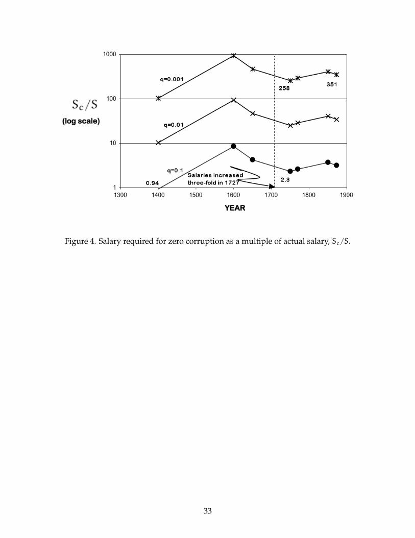
Figure 4. Salary required for zero corruption as a multiple of actual salary, Sc/S.

33

Tabl

e1.

Popu

lati

on,l

and

and

esti

mat

edra

tio

ofpo

tent

ialc

orru

ptin

com

eto

sala

ry.

Year

Popu

lati

on,N

*C

ulti

vate

dLa

nd,T

*N

/N

1873

T/T

1873

S/S

1873

**B/S

(mill

ion)

(mill

ion

shih

mou

)14

0065

-80

300

-440

0.20

-0.2

50.

24-0

.38

0.67

3.4

-7.3

1600

120

-200

570

-770

0.37

-0.6

20.

45-0

.66

0.33

33.6

-83.

116

5010

0-1

5050

0-7

000.

31-0

.46

0.40

-0.6

00.

3314

.3-3

3.7

1750

200

-250

800

-100

00.

62-0

.77

0.63

-0.8

61.

008.

7-1

7.6

1770

245

-295

850

-105

00.

75-0

.91

0.67

-0.9

11.

0010

.1-1

9.8

1850

385

-435

1160

-126

01.

18-1

.34

0.92

-1.0

91.

0015

.0-2

6.9

1873

325

-375

1160

-126

01.

001.

001.

0014

.0-2

1.9

*So

urce

:Wan

g(1

973,

Tabl

e1.

1),P

erki

ns(1

969,

Tabl

eII

.I).

**Ta

king

the

leve

lof

sala

ries

in18

73as

the

base

,w

eas

sum

eth

atth

isw

asth

esa

me

leve

lfr

om17

50to

1873

.In

1727

sala

ries

wer

ein

crea

sed

thre

e-fo

ldm

akin

gsa

lari

esin

1650

abou

ton

e-th

ird

the

1873

leve

l.H

isto

rica

levi

denc

esu

gges

tsth

atts

alar

ies

decr

ease

dby

aha

lffr

omab

out1

400

to15

00.W

eas

sum

eth

atsa

lari

esw

ere

unch

ange

dfr

om15

00-1

650.

34