Hierarchical tensors for the solution of high-dimensional partial ...

Hierarchical Tensor Representations

R. Schneider (TUB Matheon)

Paris 2014

Acknowledgment

DFG Priority program SPP 1324

Extraction of essential information from complex data

Co-workers: T. Rohwedder (HUB), A. Uschmajev (EPFLLaussanne)W. Hackbusch, B. Khoromskij, M. Espig (MPI Leipzig), I.Oseledets (Moscow) C. Lubich (Tubingen), O. Legeza (Wigner I- Budapest), Vandereycken (Princeton), M. Bachmayr, L.Grasedyck (RWTH Aachen), ...J. Eisert (FU Berlin - Physics), F. Verstraete (U Wien), Z.Stojanac, H. RauhhutStudents: M. Pfeffer, S. Holtz ...

I.High-dimensional problems

PDE’s in Rd , (d >> 3)Equations describing complex systems with multi-variatesolution spaces, e.g.B stationary/instationary Schrodinger type equations

i~∂

∂tΨ(t ,x) = (−1

2∆ + V )︸︷︷︸H

Ψ(t ,x), HΨ(x) = EΨ(x)

describing quantum-mechanical many particle systemsB stochastic SDEs and the Fokker-Planck equation,

∂p(t , x)∂t

=d∑

i=1

∂

∂xi

(fi(t , x)p(t , x)

)+

12

d∑i,j=1

∂2

∂xi∂xj

(Bi,j(t , x)p(t , x)

)describing mechanical systems in stochastic environment,

x = (x1, . . . , xd ), where usually, d >> 3!

B parametric PDEs (arising in uncertainty quantification)

e.g. ∇xa(x , y1, . . . , yd )∇xu(x , y1, . . . , yd ) = f (x)

x ∈ Ω , y ∈ Rd , + b.c. on ∂Ω .

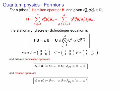
Quantum physics - FermionsFor a (discs.) Hamilton operator H and given hq

p ,gr ,sp,q ∈ R,

H =d∑

p,q=1

hqpaT

p aq +d∑

p,q,r ,s=1

gp,qr ,s aT

r aTs apaq .

the stationary (discrete) Schrodinger equation is

HU = EU , U ∈d⊗

j=1

C2 ' C(2d ) .

where A :=

(0 10 0

), AT =

(0 01 0

)S :=

(1 00 −1

),

and discrete annihilation operators

ap ' ap := S ⊗ . . .⊗ S ⊗ A(p) ⊗ I ⊗ . . .⊗ I

and creation operators

a†p ' aTp := S ⊗ . . .⊗ S ⊗ AT

(p) ⊗ I ⊗ . . .⊗ I

Curse of dimensionsFor simplicity of presentation: discrete tensor product spaces

H = Hd :=⊗d

i=1 Vi , e.g.: V =⊗d

i=1 Rni = R(Πdi=1ni )

we consider tensors as multi-index arrays (Ii = 1, . . . ,ni )

U =(Ux1,x2,...,xd

)xi =1,...,ni , i=1,...,d ∈ V ,

or equivalently functions of discrete variables (K = R or C)

U : ×di=1Ii → K , x = (x1, . . . , xd ) 7→ U = U[x1, . . . , xd ] ∈ H ,

d = 1: n-tuples (Ux )nx=1, or x 7→ U[x ], or d = 2: matrices

(Ux,y

)or (x , y) 7→ U[x , y ].

If not specified otherwise, ‖.‖ =√〈., .〉 denotes the `2- norm.

dim Hd = O(nd ) −− Curse of dimensionality!

e.g. n = 100,d = 10 10010 basis functions, coefficient vectors of 800× 1018 Bytes = 800 Exabytes

n = 2, d = 500: then 2500 >> the estimated number of atomsin the universe!

Setting - Tensors of order dGoal: Problems posed on tensor spaces,

H :=⊗d

i=1 Vi , e.g.: H =⊗d

i=1 Rn = R(nd )

Notation: x = (x1, . . . , xd ) 7→ U = U[x1, . . . , xd ] ∈ H Forsimplicity we will consider only the Hilbert spaces `2(I)!

Main problem:

dim V = O(nd ) −− Curse of dimensionality!


Approach: Some higher order tensors can be constructed(data-) sparsely from lower order quantities.

As for matrices, incomplete SVD:

A[x1, x2] ≈r∑

k=1

σk(uk [x1]⊗ vk [x2]

)

Setting - Tensors of order dGoal: Problems posed on tensor spaces,

H :=⊗d

i=1 Vi , e.g.: H =⊗d

i=1 Rn = R(nd )

Notation: x = (x1, . . . , xd ) 7→ U = U[x1, . . . , xd ] ∈ H Forsimplicity we will consider only the Hilbert spaces `2(I)!

Main problem:

dim V = O(nd ) −− Curse of dimensionality!


Approach: Some higher order tensors can be constructed(data-) sparsely from lower order quantities.

Canonical decomposition for order-d-tensors:

U[x1, . . . , xd ] ≈r∑

k=1

(⊗d

i=1 ui [xi , k ]).

I.Subspace approximation and novel

tensor formats

1,2,3,4,5B

4,5

U4 5 U

B

B

B

U

UU

3

2 1

1,2,3

1,2

U1,2

U1,2,3

(Format h representation closed under linear algebra manipulations)

Subspace approximation d = 2Let F : K → V , y 7→ Fy ∈ V and K be compact. (Provided itmake sense,) the Kolmogorov r -width is

dr ,∞(F ) := infU:dim U ≤r ,U⊂V

supy∈Kinffy∈U‖Fy − fy‖

dr ,2(F ) := infU:dim U ≤r ,U⊂V

( ∫K

inffy∈U‖Fy − fy‖2dy) 1

2

Theorem (E. Schmidt (07))V := Rn1 , K := 1 . . . ,n2, (x , y)→ Fy (x) := U[x , y ] ∈ Rn1×n2 ,then the best approximation in the library of all subspaces ofdimension at most r is provided by the singular valuedecomposition (SVD, Schmidt decomposition) and

dr ,2(F ) = infV∈U1⊗U2:U1⊂Rn1 ,U2⊂Rn2 ; dim U1≤r

‖U− V‖

Tucker decomposition - sub-space approximation

We are seeking subspaces Ui ⊂ Vi fitting best to a given tensorX ∈

⊗di=1 Vi , in the sense

‖X − U‖2 := infV∈U1⊗···⊗Ud : dim Ui≤ri‖X − V‖2

i.e we are minimizing over subspaces Ui ∈ G(Vi , ri),

G(V , r) := U ⊂ V subspace : dim U = r Grasmannian

Ui = span biki

: ki = ri ⊂ Vi , rank tuple r = (r1, . . . , rd ) .

⇒ C[k1, . . . , kd ] = 〈U,b1k1⊗ · · · ⊗ bd

kd〉 core tensor

U[x1, .., xd ] =

r1∑k1=1

. . .

rd∑kd =1

C[k1, .., kd ]d⊗

i=1

biki

[xi ]

Subspace approximation

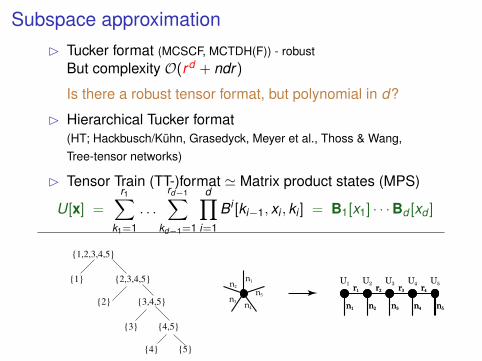
Subspace approximationB Tucker format (MCSCF, MCTDH(F)) - robust

But complexity O(rd + ndr)

Is there a robust tensor format, but polynomial in d?

Univariate bases xi 7→(Ui [ki , xi ]

)riki =1 (→ Graßmann man.)

U[x1, .., xd ] =

r1∑k1=1

. . .

rd∑kd =1

B[k1, .., kd ]d⊗

i=1

Ui [ki , xi ]

1,2,3,4,5

1 2 3 54

Subspace approximationB Tucker format (MCSCF, MCTDH(F)) - robust

But complexity O(rd + ndr)

Is there a robust tensor format, but polynomial in d?

B Hierarchical Tucker format(HT; Hackbusch/Kuhn, Grasedyck, Meyer et al., Thoss & Wang,Tree-tensor networks)

B Tensor Train (TT-)format ' Matrix product states (MPS)

U[x] =

r1∑k1=1

. . .

rd−1∑kd−1=1

d∏i=1

Bi [ki−1, xi , ki ] = B1[x1] · · ·Bd [xd ]

1,2,3,4,5

1 2,3,4,5

2 3,4,5

4,5

5

3

4

U1 U2 U3 U4 U5

r1 r2 r3 r4

n1 n2 n3 n4 n5

Hierarchical tensor (HT) formatB Canonical decompositionB Subspace approach (Hackbusch/Kuhn, 2009)

(Example: d = 5,Ui ∈ Rn×ki ,Bt ∈ Rkt×kt1×kt2 )

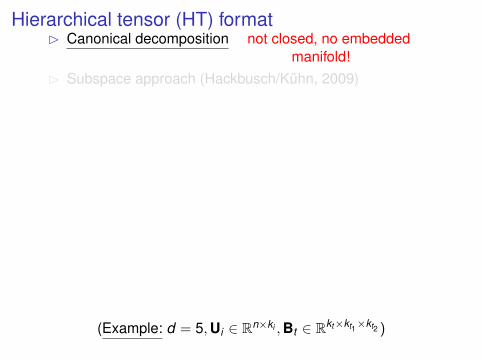
Hierarchical tensor (HT) formatB Canonical decomposition not closed, no embedded

manifold!B Subspace approach (Hackbusch/Kuhn, 2009)




1,2,3,4,5B

4,5

U4 5 U

B

B

B

U

UU

3

2 1

1,2,3

1,2




1,2,3,4,5B

4,5

U4 5 U

B

B

B

U

UU

3

2 1

1,2,3

1,2

U1,2




1,2,3,4,5B

4,5

U4 5 U

B

B

B

U

UU

3

2 1

1,2,3

1,2

U1,2

U1,2,3


Recursive definition by bases representations

Uα = spanb(α)i : 1 ≤ irα

b(α)` =

rα1∑i=1

rα2∑j=1

cα[i , j`] b(α1)i ⊗ b(α2)

j (α1, α2 sons of α ∈ TD).

The tensor is recursively defined by the transfer or componenttensors (`, i , j) 7→ cα[i , j , `] in Rkt×k1×k2 .

U[x] =∑

kα:α∈T

⊗α∈T

cα[ks1(α), ks2(α), kα]

(with obvious modifications for α = D or α is a leave.)Data complexity O(dr3 + dnr) ! (r := maxrα)

TT - Tensors - Matrix product representationNoteable special case of HT:

TT format (Oseledets & Tyrtyshnikov, 2009)' matrix product states (MPS) in quantum physics Affleck,

Kennedy, Lieb &Tagasaki (87)., Rommer & Ostlund (94), Vidal (03),HT ' tree tensor network states in quantum physics (Cirac, Verstraete, Eisert ..... )

TT tensor U can be written as matrix product form

U[x] = U1[x1] · · ·Ui [xi ] · · ·Ud [xd ]

=

r1∑k1=1

..

rd−1∑kd−1=1

U1[x1, k1]U2[k1, x2, k2]...Ud−1[kd−2xd−1, kd−1]Ud [kd−1, xd , kd ]

with matrices or component functions

Ui [xi ] =(uki−1,ki [xi ]

)∈ Rri−1×ri , r0 = rd := 1 .

Redundancy: U[x6 = U1[x1]GG−1U2[x2] · · ·Ui [xi ] · · ·Ud [xd ] .

HSVD - hierarchical (and high order) SVD

- Vidal (2003), Oseledets (2009), Grasedyck (2009), Kuhn (2012)

Matricisation or unfolding(x1, . . . , xd ) 7→ A(x1),(x2,...,xd ) = U[x] ∈ V1 ⊗ V ∗2 ⊗ · · ·V ∗d

The tensor x→ U[x]

U[x1, . . . , xd ] = U1[x1] · · ·Ui [xi ] · · ·Ud [xd ]

=

r1∑k1=1

. . .

rd−1∑kd−1=1

U1[x1, k1]U2[k1, x2, k2] . . .Ud−1[kd−2xd−1, kd−1]Ud [kd−1, xd ]


Ui [xi ] = (Ui [ki−1, xi , ki ]) ∈ Rri−1×ri , r0 = rd := 1 .

Hard thresholding Hs(U): s1 ≤ r1; truncate the above sumsafter s1.

HSVD - hierarchicalSVD


Matricisation or unfolding(x1, . . . , xd ) 7→ A(x1,x2),(x3,...,xd ) = U[x] ∈ V1 ⊗ V2 ⊗ V ∗3 ⊗ · · ·V ∗d


U[x1, . . . , xd ] = U1[x1] · · ·Ui [xi ] · · ·Ud [xd ]

=

r1∑k1=1

. . .

rd−1∑kd−1=1

U1[x1, k1]U2[k1, x2, k2]. . .Ud−1[kd−2xd−1, kd−1]Ud [kd−1, xd ]



Hard thresholding Hs(U): si ≤ ri ; truncate the above sums aftersi , i = 1, . . . ,d − 1.

HSVD - hierarchical (and high order) SVD


Matricisation or unfolding(x1, . . . , xd ) 7→ A(x1...,xd−1),(xd ) = U[x] ∈ V1 ⊗ · · ·Vd−1 ⊗ V ∗d


U[x1, . . . , xd ] = U1[x1] · · ·Ui [xi ] · · ·Ud [xd ]

=

r1∑k1=1

. . .

rd−1∑kd−1=1

U1[x1, k1]U2[k1, x2, k2] . . .Ud−1[kd−2xd−1, kd−1]Ud [kd−1, xd ]



Data Complexity: O(ndr2), r = maxri : i = 1, . . . ,d − 1,

Complexity of HSVDLet us assume that

U[x1, . . . , xd ]

=

R1∑k1=1

. . .

Rd−1∑kd−1=1

U1[x1, k1] · · · Ud−1[kd−2, xd−1, kd−1]Ud [kd−1, xd ]

For i = 1, . . . , d − 1 compute,

U i [ki−1, xi , ki ] :=

Ri∑ki−1=1

Vi−1[ki−1, ki−1]Ui [ki−1, xi , ki ]

we decompose

U i [ki−1, ni , ki ] =

ri∑ki =1

Ui [ki−1, ni , ki ]Vi [ki , ki ]

Computational costs are O(dn2r2R2)

ExampleAny canonical representation with r terms

r∑k=1

U1(x1, k) · · ·Ud (xd , k)

is also TT with ranks ri ≤ r , i = 1, . . . ,d − 1.But conversely canonical r term representation is bounded byr1 × · · · × rd−1 = O(rd−1)Hierarchical ranks could be much smaller than canonical rank.Example xi ∈ [−1,1], i = 1, . . . ,d , i.e r = d ,

U(x1, . . . , xd ) =d∑

i=1

xd = x1 ⊗ I · · ·+ I ⊗ x2 ⊗ I ⊗ · · · ,

but

U(x1, . . . , xd ) = (1, x1)

(1 x20 1

)· · ·(

1 xd−10 1

)(xd1

)here r1 = . . . = rd−1 = 2.

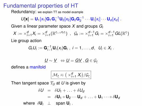
Fundamental properties of HTRedundancy: we explain TT as model example

U[x] = U1[x1]G1G−11 U2[x2]G2G−1

2 · · ·Ui [xi ] · · ·Ud [xd ] .

Given a linear parameter space X and groups Gi

X := ×di=1Xi = ×d

i=1(Rri−1ni ri ) , Gr := ×d−1i=1 Gi = ×d−1

i=1 GL(Rri )

Lie group action

GiUi := G−1i−1Ui(xi)Gi , i = 1, . . . ,d , Ui ∈ Xi .

U ∼ V ⇔ U = GV ,G ∈ Gr

defines a manifold

Mr h(×d

i=1 Xi)/Gr

Then tangent space TU at U is given by

δU = δU1 + . . .+ δUd

= δU1 U2 · · ·Ud + . . .+ U1 · · · δUd

where δUi ⊥ span Ui .

M≤r =⋃

si≤ri

Ms =Mr ⊂ H is (weakly) closed! Hackbusch & Falco

Observation: matrix ranks r are upper semi-continuous!

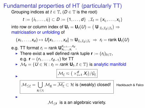
Fundamental properties of HT (particularly TT)Grouping indices at t ∈ T, (D ∈ T is the root)

t := i1, . . . , il ⊂ D := 1, . . . ,d , It = xi1 , . . . , xil

into row or column index of Ut = Ut (U) =(

U It ,ID\It

)⇒

matricisation or unfolding of

(x1, . . . , xd ) 7→ U[x1, . . . , xd ] ' UIt ,ID\It ⇒ rt = rank Ut (U)

e.g. TT format ri = rank Uxi+1,...,xdx1,...,xi

.I There exist a well defined rank tuple r := (rt )t∈T,

e.g. r = (r1, . . . , rd−1) for TTI Mr = U ∈ H : rt = rank Ut , t ∈ T is analytic manifold

Mr h(×d

i=1 Xi)/Gr

I

M≤r =⋃

si≤ri

Ms =Mr ⊂ H is (weakly) closed! Hackbusch & Falco

I

M≤r is a an algebraic variety.

Table: Some comparison

canonical Tucker HTcomplexity O(ndr) O(rd + ndr) O(ndr + dr3)

TT- O(ndr2)++ – +

rank no defined definedrc ≥ rT rT ≤ rHT ≤ rc

(weak) closedness no yes yesessential redundancy yes no noembedded manifold no yes yes

dyn. low rank approx. no yes yesrecovery ?? yes yes

quasi best approx. no yes yesbest approx. no exist exist

but NP hard but NP hard

M≤r is an algebraic variety?! Not included here are general tensor

networks, MERA etc.

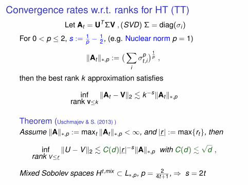
Convergence rates w.r.t. ranks for HT (TT)Let At = UT ΣV , (SVD) Σ = diag(σi)

For 0 < p ≤ 2, s := 1p −

12 , (e.g. Nuclear norm p = 1)

‖At‖∗,p :=(∑

i

σpt ,i

) 1p ,

then the best rank k approximation satisfies

infrank V≤k

‖At − V‖2 . k−s‖At‖∗,p

Theorem (Uschmajev & S. (2013) )

Assume ‖A‖∗,p := maxt ‖At‖∗,p <∞, and |r | := maxrt, then

infrank V≤r

‖U − V‖2 . C(d)|r |−s‖A‖∗,p with C(d) .√

d ,

Mixed Sobolev spaces H t ,mix ⊂ L∗,p, p = 24t+1 ,⇒ s = 2t

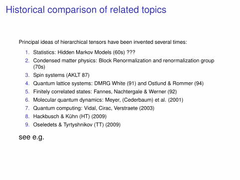
Historical comparison of related topics

Principal ideas of hierarchical tensors have been invented several times:

1. Statistics: Hidden Markov Models (60s) ???

2. Condensed matter physics: Block Renormalization and renormalization group(70s)

3. Spin systems (AKLT 87)

4. Quantum lattice systems: DMRG White (91) and Ostlund & Rommer (94)

5. Finitely correlated states: Fannes, Nachtergale & Werner (92)

6. Molecular quantum dynamics: Meyer, (Cederbaum) et al. (2001)

7. Quantum computing: Vidal, Cirac, Verstraete (2003)

8. Hackbusch & Kuhn (HT) (2009)

9. Oseledets & Tyrtyshnikov (TT) (2009)

see e.g.

Contributions about hierarchical tensors

I HT - Hackbusch & Kuhn (2009), TT - Oseledets & Tyrtyshnikov (2009)I MPS- Affleck et al. AKLT (Affleck, Kennnedy, Lieb, Takesaki 1987), Fannes,

Nachtergale & Werner (92), DMRG- S: White (91),I HOSVD-Laathawer et.al. (2001), HSVD Vidal (2003), Oseledets (09), Grasedyck

(2010), Kuhn (2012)I Riemannian optimization - Absil et al. (2008), Lubich, Koch, Conte, Rohwedder,

S. Uschmajew, Vandereycken, Kressner, Steinlechner, Arnold & Jahnke, ...I Oseledets, Khoromskij, Savostyanov, Dolgov, Kazeev, ...I Grasedyck, Ballani, Bachmayr, Dahmen, ...I Falco, Nouy, Ehrlacher ....I Physics: Cirac, Verstraete, Schollwock, Legeza, G. Chan, Eisert, ......

II.How to compute with hierarchical

tensors

U M

X = F(X).

U = PUF(U).

F(U) TUM

PLOTSUNDLOGOS/fig−ttmc.pdf

Computation in hierarchical tensor format - HTarithmetics

Given a tree T, all tensors U,V ∈Ms for some multilinear ranks. Then

1. U + V ∈M≤2s

2. x 7→ U[x]V [x] ∈M≤s2 Hadamard product

3. 〈U,V 〉 can be performed in O(ndr2 + dr4) resp. O(ndr3)(TT) arithmetic operations

4. operators A : H → H may be written in canonical, TT orHT format.

5. Assumption AU is accessible as a rank S HT tensor.Remark: E.g. A + U can be recovered into a standard form byHSVD, or approximated.

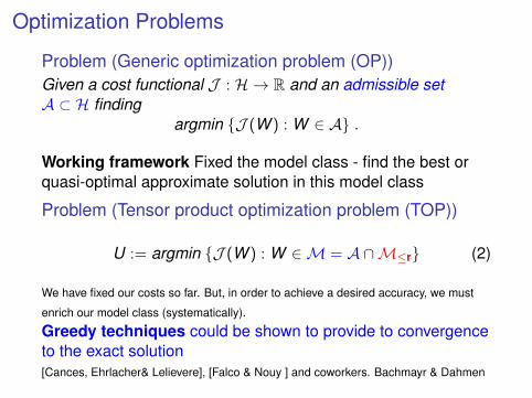
Optimization Problems

Problem (Generic optimization problem (OP))Given a cost functional J : H → R and an admissible setA ⊂ H finding

argmin J (W ) : W ∈ A .

Working framework Fixed the model class - find the best orquasi-optimal approximate solution in this model class

Problem (Tensor product optimization problem (TOP))

U := argmin J (W ) : W ∈M = A ∩M≤r (1)

Admissible set is confined toM≤r - tensors of rank at most r.

WARNING: Hillar & Lim (2011):Most tensor problems are NP hard if d ≥ 3.

for example: best rank 1 approximation (multiple local minima).

Optimization Problems

Problem (Generic optimization problem (OP))Given a cost functional J : H → R and an admissible setA ⊂ H finding

argmin J (W ) : W ∈ A .

Working framework Fixed the model class - find the best orquasi-optimal approximate solution in this model class

Problem (Tensor product optimization problem (TOP))

U := argmin J (W ) : W ∈M = A ∩M≤r (2)

We have fixed our costs so far. But, in order to achieve a desired accuracy, we must

enrich our model class (systematically).

Greedy techniques could be shown to provide to convergenceto the exact solution[Cances, Ehrlacher& Lelievere], [Falco & Nouy ] and coworkers. Bachmayr & Dahmen

ExampleEspig,Hackbusch, Rohwedder & Schneider (2010)

1. Approximation: for given U ∈ H minimize

J (W ) = ‖U −W‖2 , W ∈M

2. solving equations: where A, g : V → H,

AU = B or g(U) = 0

hereJ (W ) := ‖AW − B‖2

∗ resp. F (W ) := ‖g(W )‖2∗ .

3. or, if A : V → V ′ is symmetric and B ∈ V ′, V ⊂ H ⊂ V ′,

J (W ) :=12〈AW ,W 〉 − 〈B,W 〉

4. computing the lowest eigenvalue of a symmetric operator A : V → V ′,

U = argmin J (W ) = 〈AW ,W 〉 : 〈W ,W 〉 = 1 .

In many cases A ∩M≤r =M≤r .

Hard Thresholding -Projected Gradient Algorithms: E.G. inimize

J (U) :=12〈UAU〉 − 〈U,Y 〉 ∇J(X ) = (AU − Y )

w.r.t. low rank constraints

V n+1 := Un − αn(C−1(AUn − Y )

)gradient step

Un+1 := Rn(V n+1) .

Rn (nonlinear) projection to model class

Rn : Rn1×n2 →Mr

e.g HSVD σs := σst singular values of Vt = Vt (V n+1), t ∈ T,1. Hard thresholding, σs := 0, s > r , σs ← σs, s ≤ r2. Riemannian techniques including ALS:3. Soft thresholding, σs ← maxσs − ε,0

Hard Thresholding - Riemannian gradient iteration

J (U) :=12〈U,AU〉 − 〈U,Y 〉 , ∇J (X ) = (AU − Y )

V n+1 := Un − PTUαn(C−1(AUn − Y )

)projected gradient step

= Un + ξn , Mr + TU

Un+1 := Rn(V n+1) := R(Un, ξn) .

PTU : H → TU orthogonal projection onto tangent space at Uretraction (Absil et al.) R(U, ξ) : TMr →Mr,

R(U, ξ) = U + ξ +O(‖ξ‖2)

e.g. R is an approximate exponential map

Nonlinear Gauss Seidel local optimization for TT (HT)tensors

Alternating Linear Scheme - ALS

Relaxation (see e.g. Gauss-Seidel, ALS):For j = 1, . . . ,d :

1. fix all component tensors Uν , ν ∈ 1, . . . ,d\j, exceptindex j .

2. Optimize Uj [kj−1, xj , kj ], and orthogonalize left3. Repeat with Uj+1 (the tree is reorder to optimize alway the root!)

Repeat the relaxation procedure (in the opposite direction. )ju

u

j+1

S. Holtz, Rohwedder & Schneider (2010), Uschmajew & Rohwedder (2011),

Uschmajew & Schneider (in prep.)This is the single site DMRG algorithm!

ALS (single site DMRG) - Nonlinear Gauß SeidelSolving: AU = B, (AT = A)

U = argmin12〈AU,U〉 − 〈B,U〉 : U ∈Mr ,

U[x] = U1[x1] · · ·Ui [xi ] · · ·Ud [xd ]

Optimizing Ui , resp. Ui [ki−1, xi , ki ] leads to a linear system

AiUi = Bi , in the small (sub-) space Rri−1×ni×ri

Renormalization group

Ai =∑ν

Li,ν ⊗ Ai,ν ⊗ Ri,ν

Li,ν ∈ Rri−1×ri−1 ,Ai,ν ∈ Rni×ni Ri,ν ∈ Rri×ri

Riemannian gradient iteration - Local ConvergenceTheorem (Local convergence of Riemaniann gradientiteration )Let V n+1 := Un + C−1(Y −AUn), assume that A is SPD andU ∈Mr. If

‖U − Um‖ ≤ δ , δ ∼ dist(U, ∂Mr)

sufficiently small, and δ ∼ dist(U, ∂Mr), then, there exist0 < ρ < 1 s.t the series Un ∈M≤r converges linearly to aunique solution U ∈M≤r with rate ρ

‖Un+1 − U‖ ≤ ρ‖Un − U‖

Remark: Suppose ‖U‖ = 1 then

dist(U, ∂Mr) ≤ mint∈T,0<k≤rt

σt ,k

is smallest (non-zero) singular value of Ut (U)!

Iterative Hard Thresholding - Local Convergence

Theorem (Global convergence of IHT)Let V n+1 := Un + C−1(Y −AUn), and Un+1 = HrV n+1 assumethat

γ‖V‖2 ≤ 〈C−1AV ,V 〉 ≤ Γ‖V‖2

with e.g. Γγ < C(d) suff. small.

Then, there exist 0 < ρ < 1 s.t the series Un ∈M≤rconvergences linearly to a unique tensor Uε ∈M≤r with rate ρ

‖Un+1 − Uε‖ ≤ ρ‖Un − Uε‖

and Uε is a quasi-optimal solution

‖U − Uε‖ ≤ CinfV∈Mr‖V − Uε‖

Iterative Hard Thresholding - Local Convergence

Theorem (Global convergence of Riemannian gradientiteration- (ongoing joint work with A. Uschmajew) )Let V n+1 := Un + C−1(Y −AUn), and A is SPD. Then, theseries Un ∈M≤r converges to a stationary point U ∈M≤r.The same results holds for the Gauß Southwell variant of ALS(1site DMRG).Lojasiewicz (-Kurtyka) inequality

J (V )θ − J (U)θ ≤ Γ‖grad J (V )‖ , 0 < θ ≤12, ‖UV ‖ ≤ δ .

LK inequality is valid on algebraic sets, o-minimal structures etc. [Bolte et al.]. It is apowerful mathematical tool for proving convergence.

1. θ = 12 : linear convergence ‖Un − U‖ . qn‖U1 − U0‖, q < 1.

2. 0 < θ < 12 : ‖Un − U‖ . n−

θ2−θ

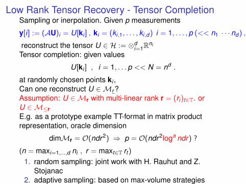
Low Rank Tensor Recovery - Tensor CompletionSampling or inerpolation. Given p measurements

y[i] := (AU)i = U[ki ] , ki = (ki,1, . . . , ki,d ) i = 1, . . . ,p (<< n1 · · · nd ) ,

reconstruct the tensor U ∈ H := ⊗di=1R

ni

Tensor completion: given values

U[ki ] , i = 1, . . .p << N = nd .

at randomly chosen points ki ,Can one reconstruct U ∈Mr ?Assumption: U ∈Mr with multi-linear rank r = (ri)t∈T. orU ∈M≤rE.g. as a prototype example TT-format in matrix productrepresentation, oracle dimension

dimMr = O(ndr2) ⇒ p = O(ndr2loga ndr) ?

(n = maxi=1,...,d ni , r = maxt∈T rt )

1. random sampling: joint work with H. Rauhut and Z.Stojanac

2. adaptive sampling: based on max-volume strategiesOseledets, Sebastinanov. Ballani, Kluge, Grasedyck(impressive)

Iterative Hard ThresholdingProjected Gradient Algorithms: Minimize residual

J(U) :=12〈AU − y,AU − y〉 ∇J(X ) = AT (AU − y)

w.r.t. low rank constraints

Y n+1 := Un − αn(AT (AUn − y)

)gradient step

Un+1 := Rn(Y n+1) .

Rn (nonlinear) projection to model class

Rn : Rn1×n2 →Mr

e.g HSVD σs := σst singular values of Yt = Yt (Y n+1), t ∈ T,1. Hard thresholding, σs := 0, s > r , σs ← σs, s ≤ r compressive

sensing: Blumensath et al. , matrix recovery : Tanner et al.

2. Riemannian techniques including ALS: e.g. Kressner et al. (2013), da

Silva & Herrmann (2013)

We obtain first, similar convergence results based on TensorRIP.

Convex framework for tensor product approximation -in preparation

or can we learn from Compressive Sensing?We want to find

Ur ∈ V ∈ Hd : ‖U − V‖ ≤ ε , where AU − Y = 0 .

with minimal ranks (`0-norm) i.e. we are minimize your costs.(fixing our accuracy) In compressive sensing `0 is relaxed by`1-norm.Soft Thresholding [Daubechies, Defrise, DelMol (2004)] (linear)convergence but only to the minimizer of, e.g. d = 2

ε‖U‖∗,1 + ‖∇J (U)‖2

(Bachmayr & S.) work under construction

Iterative Hard Thresholding - Remarks

I IHT converges only if the pre-conditioner is sufficiently good. Convergence islinear.

I IHT can be easily combined with enrichment strategies (r ↑ (see also Bachmayr /Damen)

I RGI is fast (avoiding large HSVD), but only to local minimizers.I RGI requires special care at singular point (where s < r).I Good preconditioners can speed up the convergence of RGII Subspace accelerations like CG, BFGS, DIIS, Anderson are powerful using an

appropriate vector transport (i.e. transporting previous tangent vectors to thenew tangential space) (Pfeffer 2014, Vandereycken, Haegemann et al. (CG) )

PracticallyI good initial guesses are importantI RGI must be combined with enrichment strategies, e.g. greedy techniques,

two-site DMRG or AMEN (Sebastianov et al.)

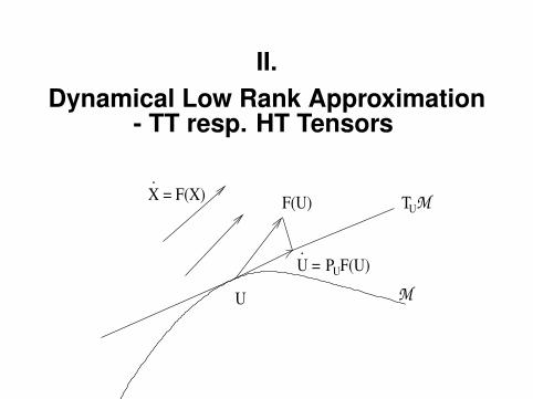
II.Dynamical Low Rank Approximation

- TT resp. HT Tensors

U M

X = F(X).

U = PUF(U).

F(U) TUM

Dirac Frenkel principleM⊆ VB for optimisation tasks J (U)→ min:

Solve first order condition J ′(U) = 0 on tangent space,

〈J ′(U),V 〉 = 0 ∀V ∈ TU .

(Dirac-Frenkel variational principle, Absil et al., Q.Chem.: MCSCF, . . . )

J’(U) = X − U

X

U M

T UM

Dirac Frenkel principleM⊆ VB for differential equations X = f (X ),X (0) = X0:

Solve projected DE, U = PU f (U),U(0) = X0 ∈M,

〈U(t),V 〉 = 〈f (U(t)),V 〉 ∀V ∈ TU(t) .

(Dirac-Frenkel variational principle, Lubich et al., Q.Chem.: TDMCH . . . )

U M

X = F(X).

U = PUF(U).

F(U) TUM

Convergence estimates

Time-dependent equations:

∂

∂tU = AU + F (U) , U(0) = U0 ∈Mr ,

A =∑d

i=1 I ⊗ · · · I ⊗ Ai ⊗ I · · · , Ai = H10 (Ω) ∩ H2(Ω)→ L2(Ω).

B Quasi-optimal error bounds(Lubich/Rohwedder/Schneider/Vandereycken)A = 0, 0 ≤ t < T solution X (t) with approx. U(t) ∈Mr,X (0) = U(0),

‖U(t)− Ubest(t)‖

. ‖Ψ(t)− V (t)‖+ tL∫ t

0

(inf

V (s)∈Mr‖Ψ(s)− V (s)‖+ ε

)ds

IV.

Appendix: Tensorization(and second quantization)

Vector-tensorization - e.g. binary coding1D example: vector, e.g. signal or function g : [0,1]→ R,

k → f (k) ,

(or g(

k2d )

), k = 0, . . . ,2d − 1 .

Labeling of indices k ' µ ∈ I by an binary string of length d ,

µ = µ(k) = (0,0,1,1,0, . . .) 'd−1∑j=0

µi2j = k(µ) , µi = 0,1 .

Tensorization

µ 7→ U(µ) := f (k(µ)) ∈d−1⊗j=0

R2 , ord−1⊗j=0

C2.

This provides an isomorphm T : R2d ↔⊗d−1

j=0 R2 by Tf := U.So far no information is lost, N = 2d or d = log2 N.

Binary coding - signal compression - 1 D functionsQuantized TT - Oseledets (2009), Khoromskij (2009) :TT approximation of UI Storage complexity N is reduced to 2r2 log2 N! (linear in

d = log2 N)I Allow e.g extreme fine grid size h = o(ε) = 2−d = 1

N .Examples:

1. For Kronecker δi,j (Dirac function) is r = 1.2. For plane wave (fixed k =

∑dj=1 νj2j−1)

e2πik = e2πi∑d

j=1 νj 2j−1= Πd

j=1e2πiνl 2j−1, νj = 0,1,

again (complex) r = 1, or (real r = 2) .

Theorem (Grasedyck)Let ε > 0. If g : [0,1]→ R is piecewise analytic, forri ≥ − logα ε, N ∼ ε−τ , there is a TT tensor Uε of rank ≤ r s.t.

‖U − Uε‖ . ε , dr2 . log2α+1 N .

Examples: TT approximation of tensorized functionsAiry function: f (x) = x1/4 sin 2x2/3

3 , chirp: f (x) = sin x4 cos(x2)

and f (x) = sin 1x

0 20 40 60 80 100−1

−0.5

0

0.5

1

x

y

x−1/4

sin(2/3 x3/2

)

10 12 14 16 18 20

−1

−0.5

0

0.5

1

x

y

sin(x/4) cos(x2)

0 0.2 0.4 0.6 0.8 1

−1

−0.5

0

0.5

1

x

y

sin(1/x)

3 5 10 15 20 220

10

16

20

24

30

40

50

60

d

ma

x.

ran

k

x−1/4

sin(2/3 x3/2

), x∈ ]0,100[

sin(1/x), x∈ ]0,1[

sin(x/4) cos(x2), x∈ ]10,20[

2 4 6 8 10 12 14 16 18 200

10

20

30

40

50

60

i

r i

x−1/4

sin(2/3⋅ x3/2

), x ∈ ]0,100[

sin(1/x), x ∈ ]0,1[

sin(x/4) cos(x2), x ∈ ]10,20[

Anti-Symmetric Functions - FermionsConsider a univariate (complete) orthonormal basis

Vi := span ϕi : i = 1, . . . ,d , H =N⊗

i=1

Vi

ONB of antisymmetric functions by Slater determinants

ΨSL[k1, . . . , kN ](x1; . . . ; xN) := ϕk1(x1) ∧ . . . ∧ ϕkN (xN)

=1√N!

det(ϕki (xj , sj))Ni,j=1

VNFCI =

N∧i=1

Vi = spanΨSL = Ψ[k1, . . . , kN ] : k1 < . . . < kN ≤ d ⊂ H

Curse of dimensionality dimVNFCI =

(dN

)!

Fock spaceLet Ψµ := ΨSL[ϕk1 , . . . , ϕkN ] = Ψ[k1, . . . , kN ] basis Slater det.Labeling of indices µ ∈ I by an binary string of length d

e.g.: µ = (0,0,1,1,0, . . .) =:d−1∑i=0

µi2i , µi = 0,1 ,

I µi = 1 means ϕi is (occupied) in Ψ[. . .].I µi = 0 means ϕi is absend (not occupied) in Ψ[. . .].

(discrete) Fock space Fd is of dimFd = 2d , (K := C,R)

Fd :=d⊕

N=0

VNFCI = Ψ : Ψ =

∑µ

cµΨµ

Fd ' c : µ 7→ c(µ0, . . . , µd−1) = cµ ∈ K , µi = 0,1 =d⊗

i=1

K2

This is a basis depent formalism⇒ : Second Quantization

Discrete annihilation and creation operators

A :=

(0 10 0

), AT =

(0 01 0

)In order to obtain the correct phase factor, we define

S :=

(1 00 −1

),

and the discrete annihilation operator

ap ' ap := S ⊗ . . .⊗ S ⊗ A(p) ⊗ I ⊗ . . .⊗ I

where A(p) means that A appears on the p-th position in theproduct.The creation operator

a†p ' aTp := S ⊗ . . .⊗ S ⊗ AT

(p) ⊗ I ⊗ . . .⊗ I

Hamilton operator in second quantization

For a Hamilton operator H : VNFCI =: V → V ′

HΨ =∑ν′,ν

〈Ψν′ ,HΨν〉cνΨν′ =∑ν′

(Hc)ν′Ψν′ .

Theorem (Slater -Condon)The Galerkin matrix H of a two particle Hamilton operatoracting on Fermions is sparse and can be represented by

H =d∑

p,q=1

hqpaT

p aq +d∑

p,q,r ,s=1

gp,qr ,s aT

r aTs apaq .

Remark: In case of spin systems the 2× 2 matrices A,AT ,S, I aremost replaced by Pauli matrices - e.g. Heisenberg model etc. (-originof matrix product states (MPS) and DMRG)See also quantum information theory and quantum computing!

Particle number operator and Schrodinger eqn.

P :=d∑

p=1

a†pap , ' P :=d∑

p=1

ATp Ap .

The space of N-particle states is given by

VN := c ∈d⊗

i=1

K2 : Pc = Nc .

Variational formulation of the Schrodinger equation

c = (c(µ)) = argmin〈Hc,c〉 : 〈c,c〉 = 1 , Pc− Nc = 0 .

Table: New paradigm - discretization

traditional vs. newd fixed , n→∞ n fixed, e.g. n = 2, d →∞

Knd ⊗dj=1 K2

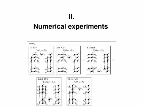
II.Numerical experiments

sweep

P1,1AP1,1u = P1,1bT T

A1

U2

=

U3

Ud-1

Ud

U2

U3

Ud-1

Ud

A2

A3

Ad-1

Ad

n1 n1r1

U1n1

r1r1

B1

U2

U3

Ud-1

Ud

B2

B3

Bd-1

Bd

n1

1st MIS

Pd-1,1APd-1,1u = Pd-1,1bT T

d+1-th MIS

rd-1rd-1

rd-1rd-1

UdUd

U2U2

A1

U1

U3

U1

U3

A2

A3

Ad-1

Ad

n1 n1

n2 n2

n3 n3

nd-1 nd-1

nd nd

=Ud-1nd-1

rd-1

rd-2

rd-1

rd-1

Ud

U2

U1

U3

nd-1

B1

B2

B3

Bd-1

Bd

2d-2-th MIS

P2,1AP2,1u = P2,1bT T

A1

U1

U3

Ud-1

Ud

U1

U3

Ud-1

Ud

A2

A3

Ad-1

Ad

r1r1

r2r2

n2 n2=

U2n2

r2

r1

B1

B2

B3

Bd-1

Bd

U1

U3

Ud-1

Ud

r1

r2

n2

P2,1AP2,1u = P2,1bT T

A1

U1

U3

Ud-1

Ud

U1

U3

Ud-1

Ud

A2

A3

Ad-1

Ad

r1r1

r2r2

n2 n2=

U2n2

r2

r1

B1

B2

B3

Bd-1

Bd

U1

U3

Ud-1

Ud

r1

r2

n2

2nd MIS

Pd,1APd,1u = Pd,1bT T

B1

B2

B3

Bd-1

Bd

U2U2

rd-1rd-1

A1

U1

U3

Ud-1

U1

U3

Ud-1

A2

A3

Ad-1

Adnd nd

=Udnd

rd-1

U2

rd-1

U1

U3

Ud-1

nd

d-th MIS

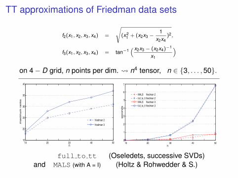
TT approximations of Friedman data sets

f2(x1, x2, x3, x4) =

√(x2

1 + (x2x3 −1

x2x4)2,

f3(x1, x2, x3, x4) = tan−1(x2x3 − (x2x4)−1

x1

)

on 4− D grid, n points per dim. n4 tensor, n ∈ 3, . . . ,50.

full to tt (Oseledets, successive SVDs)and MALS (with A = I) (Holtz & Rohwedder & S.)

Solution of −∆U = b using MALS/DMRGI Dimension d = 4, . . . ,128 varyingI Gridsize n = 10I Right-hand-side b of rank 1I Solution U has rank 13

By now, we are able to solve Fokker Planck, chemical masterequations parametric PDE’S, for moderate r < 100 andd ∼ 10− 100 with Matlab on a laptop. In QTT n = 2, d ∼ 1000.See B. Khoromskij (MPI Leipzig)

Some numerical results - e.g. Parabolic PDEsjoint work with B. Khoromskij, I. Oseledets

∂

∂tΨ = HΨ = (−1

2∆ + V )Ψ , Ψ(0) = Ψ0 .

V (x1, . . . , xd ) =12

f∑k=1

x2k +

d−1∑k=1

(x2

k xk+1 −13

x3k

).

Timings and error dependence for the modified heat equation (imaginary time) with aHenon-Heiles potential

time interval [0, 1], τ = 10−2, the manifold has ranks 10

Table: Time

Dimension Time (sec)2 2.774 21.398 64.8216 142.232 346.964 832.31

Table: Errror

τ Error1.000e-01 3.137e-035.000e-02 7.969e-042.500e-02 2.000e-041.250e-02 5.001e-056.250e-03 1.247e-053.125e-03 3.081e-061.563e-03 7.335e-07

QC-DMRG for HT - tree tensor networksrecent joint paper with Legeza, Murg, Nagy, Verstraete (in preparation)

dissoziation of a diatomic molecule LiF - first eigenvalues - tree tensor networks (HT)

2 4 6 8 10 12 14−107.15

−107.1

−107.05

−107

−106.95

−106.9

−106.85

−106.8

Bond length(r)

Sing

let e

nerg

ies

LiF, 6e25o, DMRG, m=256, ordopt, casopt

GS, S=01XS, S=02XS, S=03XS, S=0

First numerical examplesJ.M. Claros -Bachelor thesis, M. Pfeffer, TT d = 4, r = 1, 3, Stojanac-Tucker d = 3

0 100 200 300 400 500 600 700 800 900 100010−12

10−10

10−8

10−6

10−4

10−2

100

102

iterations

erro

r of

com

plet

ion

10%

20%

40%

0 100 200 300 400 500 600 700 800 900 100010−14

10−12

10−10

10−8

10−6

10−4

10−2

100

102

erro

r of

res

idua

l

10%

20%

40%

0 10 20 30 40 50 60 700

10

20

30

40

50

60

70

80

90

100

percentage of measurements

perc

enta

ge o

f suc

cess

Recovery of low!rank tensors of size 10 x 10 x 10

r=(1,1,1)r=(2,2,2)r=(3,3,3)r=(5,5,5)r=(7,7,7)

0 5 10 15 20 25 30 350

10

20

30

40

50

60

70

80

90

100

percentage of measurements

perc

enta

ge o

f suc

cess

Recovery of low!rank tensors of size 10 x 10 x 10

r=(1,1,2)r=(1,5,5)r=(2,5,7)r=(3,4,5)

Thank youfor your attention.

II.Dynamical Low Rank Approximation- Manifolds and Gauge Conditions

U M

X = F(X).

U = PUF(U).

F(U) TUM

Appendix: Manifolds and gauge conditionsKoch&Lubich (2009), Holtz/Rohwedder/Schneider (2011a), Uschmajew/Vandereycken(2012), Arnold& Jahnke (2012)Lubich/Rohwedder/Schneider/Vandereycken (2012)

B The sets of above tree (HT, TT or Tucker) tensors of fixedrank r each provide embedded submanifoldsMr of R(nd ).

B Canonical tangent space parametrization via componentfunctions Wt ∈ Ct is redundant, but unique via gaugeconditions for nodes t 6= tr , e.g.

Gt =

Wt ∈ Ct | 〈WTt ,Bt〉 resp. 〈WT

t ,Ut〉 = 0 ∈ Rkt×kt

B Linear isomorphism

E : ×t∈T Gt → TUM, E =∑t∈T

Et

Et : “node-t embedding operators”, defined via currentiterate (Ut ,Bt ).

Projector onto TUM: P = EE+.

Manifolds and gauge conditionsLubich et al. (2009), Holtz/Rohwedder/Schneider (2011a), Uschmajew/Vandereycken(2012),Lubich/Rohwedder/Schneider/Vandereycken (2012), Arnold/Jahnke (2012)

B The sets of above tree (HT, TT or Tucker) tensors of fixedrank r each provide embedded submanifoldsMr of R(nd ).

B Canonical tangent space parametrization via componentfunctions Wt ∈ Ct is redundant, but unique via gaugeconditions for nodes t 6= tr , e.g.

Gt =

Wt ∈ Ct | 〈WTt ,Bt〉 resp. 〈WT

t ,Ut〉 = 0 ∈ Rkt×kt

B Linear isomorphism

E : ×t∈T Gt → TUM, E =∑t∈T

Et

Et : “node-t embedding operators”, defined via currentiterate (Ut ,Bt ).

Projector onto TUM: P = EE+.

Manifolds and gauge conditionsLinear isomorphism

E = E(U) : ×t∈T Gt → TUM, E(U) =∑t∈T

Et (U)

E+ Moore Penrose inverse of E

Projector onto TUM: P(U) = EE+.

Theorem (Lubich/Rohwedder/Schneider/Vandereycken, Arnold/Jahnke (2012))

For tensor B,U,V; ‖U − V‖ ≤ cρ; there exists C dependingonly on n,d, such that there holds

‖(P(U)− P(V )

)B‖ ≤ Cρ−1‖U − V‖‖B‖

‖(I − P(U)

)(U − V )‖ ≤ Cρ−1‖U − V‖2 .

These are estimates for the curvature ofMr at U.

Optimization problems/differential flow

The problems

〈J ′(U),V 〉 = 0 resp. 〈U,V 〉 = 〈f (U),V 〉 ∀V ∈ TU

onM can now be re-cast into equations for components(Ut ,Bt ) representing low-rank tensor

U = τ(Ut ,Bt ) :

With P⊥t projector to Gt , embedding operator Et = EUt as

above, solve

P⊥t ETt J ′(U) = 0 resp. Ut = P⊥t E+

t f (U),

for t 6= tr , and

ETtr J′(U) = 0 resp. Ut = E+

t f (U).

for the “root” (e.g. by standard methods for nonlinear eqs.)

Convergence estimates

Time-dependent equations:

∂

∂tU = AU + F (U) , U(0) = U0 ∈Mr ,

A =∑d

i=1 I ⊗ · · · I ⊗ Ai ⊗ I · · · , Ai = H10 (Ω) ∩ H2(Ω)→ L2(Ω).

B Quasi-optimal error bounds(Lubich/Rohwedder/Schneider/Vandereycken)A = 0, 0 ≤ t < T solution X (t) with approx. U(t) ∈Mr,X (0) = U(0),

‖U(t)− Ubest(t)‖

. ‖Ψ(t)− V (t)‖+ tL∫ t

0

(inf

V (s)∈Mr‖Ψ(s)− V (s)‖+ ε

)ds

Hierarchical tensors for the solution of high-dimensional partial ...

Documents

Transcript of Hierarchical tensors for the solution of high-dimensional partial ...