
Heterogeneous Multiscale Methods: A Revie · COMMUNICATIONS IN COMPUTATIONAL PHYSICS Vol. 2, No. 3,...
84
COMMUNICATIONS IN COMPUTATIONAL PHYSICS Vol. 2, No. 3, pp. 367-450 Commun. Comput. Phys. June 2007 REVIEW ARTICLE Heterogeneous Multiscale Methods: A Review Weinan E 1, ∗ , Bjorn Engquist 2 , Xiantao Li 3 , Weiqing Ren 4 and Eric Vanden-Eijnden 4 1 Department of Mathematics and Program in Applied and Computational Mathematics, Princeton University, Princeton, NJ 08544, USA. 2 Department of Mathematics, The University of Texas at Austin, Austin, TX 78712, USA. 3 Department of Mathematics, Pennsylvania State University, University Park, PA 16802, USA. 4 Department of Mathematics, Courant Institute of Mathematical Sciences, New York University, New York, NY 10012, USA. Received 20 August 2006; Accepted 31 August 2006 Available online 5 October 2006 Abstract. This paper gives a systematic introduction to HMM, the heterogeneous mul- tiscale methods, including the fundamental design principles behind the HMM phi- losophy and the main obstacles that have to be overcome when using HMM for a particular problem. This is illustrated by examples from several application areas, in- cluding complex fluids, micro-fluidics, solids, interface problems, stochastic problems, and statistically self-similar problems. Emphasis is given to the technical tools, such as the various constrained molecular dynamics, that have been developed, in order to apply HMM to these problems. Examples of mathematical results on the error analysis of HMM are presented. The review ends with a discussion on some of the problems that have to be solved in order to make HMM a more powerful tool. AMS subject classifications: 65N30, 74Q05, 74Q20, 39A12 Key words: Multi-scale modeling, heterogeneous multi-scale method, multi-physics models, con- strained micro-scale solver, data estimation. Contents 1 Introduction 368 ∗ Corresponding author. Email addresses: [email protected] (W. E), [email protected] (B. Engquist), [email protected] (X. Li), [email protected] (W. Ren), [email protected] (E. Vanden- Eijnden) http://www.global-sci.com/ 367 c 2007 Global-Science Press
Transcript of Heterogeneous Multiscale Methods: A Revie · COMMUNICATIONS IN COMPUTATIONAL PHYSICS Vol. 2, No. 3,...

COMMUNICATIONS IN COMPUTATIONAL PHYSICSVol. 2, No. 3, pp. 367-450
Commun. Comput. Phys.June 2007
REVIEW ARTICLE
Heterogeneous Multiscale Methods: A Review
Weinan E1,∗, Bjorn Engquist2, Xiantao Li3, Weiqing Ren4 andEric Vanden-Eijnden4
1Department of Mathematics and Program in Applied and ComputationalMathematics, Princeton University, Princeton, NJ 08544, USA.2Department of Mathematics, The University of Texas at Austin, Austin, TX 78712,USA.3 Department of Mathematics, Pennsylvania State University, University Park, PA16802, USA.4 Department of Mathematics, Courant Institute of Mathematical Sciences, New YorkUniversity, New York, NY 10012, USA.
Received 20 August 2006; Accepted 31 August 2006
Available online 5 October 2006
Abstract. This paper gives a systematic introduction to HMM, the heterogeneous mul-tiscale methods, including the fundamental design principles behind the HMM phi-losophy and the main obstacles that have to be overcome when using HMM for aparticular problem. This is illustrated by examples from several application areas, in-cluding complex fluids, micro-fluidics, solids, interface problems, stochastic problems,and statistically self-similar problems. Emphasis is given to the technical tools, suchas the various constrained molecular dynamics, that have been developed, in order toapply HMM to these problems. Examples of mathematical results on the error analysisof HMM are presented. The review ends with a discussion on some of the problemsthat have to be solved in order to make HMM a more powerful tool.
AMS subject classifications: 65N30, 74Q05, 74Q20, 39A12
Key words: Multi-scale modeling, heterogeneous multi-scale method, multi-physics models, con-strained micro-scale solver, data estimation.
Contents
1 Introduction 368
∗Corresponding author. Email addresses: [email protected] (W. E), [email protected](B. Engquist), [email protected] (X. Li), [email protected] (W. Ren), [email protected] (E. Vanden-Eijnden)
http://www.global-sci.com/ 367 c©2007 Global-Science Press

368 W. E et al. / Commun. Comput. Phys., 2 (2007), pp. 367-450
2 The HMM framework 374
3 The heterogeneous multiscale finite element method 388
4 Complex fluids and microfluidics 392
5 Dynamics of solids at finite temperature 406
6 Interface problems 416
7 Stochastic ODEs with multiple time scales 419
8 Exploring statistical self-similarity: An example without scale separation 423
9 Error analysis 425
10 Limitations of HMM 437
11 Conclusions and new directions 439
1 Introduction
The heterogeneous multiscale method, or HMM, proposed in [56] is a general frameworkfor designing multiscale methods for a wide variety of applications. The name “hetero-geneous” was used to emphasize that the models at different scales may be of very differ-ent nature, e.g. molecular dynamics at the micro scale and continuum mechanics at themacro scale. Since its inception, there has been substantial progress on multiscale mod-eling using the philosophy of HMM. The HMM framework has proven to be very usefulin guiding the design and analysis of multiscale methods, and in several applications, ithelps to transform multiscale modeling from a somewhat ad hoc practice to a system-atic technique with a solid foundation. Yet more possibilities are waiting to be explored,particularly in the application areas. Many new questions of physical, numerical or ana-lytical nature have emerged. All these make HMM an extremely fruitful and promisingarea of research.
The purpose of this article is to give a coherent summary of the status of HMM. Itis our hope that this summary will help the reader to understand the design principlebehind the HMM philosophy, the main obstacles that one has to overcome when usingHMM for a particular problem, and the immediate problems that have to be solved inorder to make HMM a more powerful tool.
Just what is HMM? After all many multiscale modeling strategies discussed in theapplied communities are heterogeneous in nature, i.e. they involve models of differentnature at different scales, so what is special about HMM? Through this review we willshow that HMM is a general framework for designing multiscale methods that can beapplied to a wide variety of applications. In a nutshell, the philosophy is as follows. As-sume we are interested in studying the macroscale behavior of a problem for which themacroscale model is only partly known or is valid only on part of the physical domain.In typical situations, we either lack the detailed constitutive relation, or the macroscalemodel is invalid due to the presence of defects or localized singularities. Assume, onthe other hand, that we do have an accurate microscale model at our disposal, but it istoo expensive to abandon the macroscale model completely and only use the microscale

W. E et al. / Commun. Comput. Phys., 2 (2007), pp. 367-450 369
model. The HMM philosophy is to start with a carefully selected numerical method forthe macroscale model, as if the macroscale model is completely known and valid every-where, and then focus on the question of how to get the needed data in order to imple-ment the selected macroscale numerical method. In regions where the macroscale modelis invalid, or where constitutive relations are missing, we obtain the needed macroscaledata by solving the microscale model locally. This is the most important aspect of HMM:It is a strategy for designing multiscale algorithms that are driven by the data. Its effectivenessrests upon the fact that it allows us to make maximum use of the knowledge that we haveabout the particular problem at all scales, macro and micro, as well as the special featuresthat the problem might have, such as scale separation or self-similarity. For instance if themacro and micro time scales are separated, they are automatically decoupled in HMM.In addition, HMM also suggests a unified approach for carrying out error analysis for alarge class of multiscale problems.
Despite all that, we will also see from this review that HMM only gives us a startingpoint, applications of HMM to specific problems can be a highly non-trivial task. Issues offormulation have to be resolved and technical tools have to be developed along the way.The situation is similar to that of finite element methods: On one hand, finite elementoffers a very attractive framework for designing numerical methods for a wide variety ofproblems; on the other hand, applying this framework to a specific problem can be quitenon-trivial.
1.1 Classical and new multiscale methods
Almost all problems in science and engineering are multiscale in nature. Things are madeup of atoms and electrons at the atomic scale, and at the same time are characterized bytheir natural geometric dimensions which are usually several orders of magnitude larger.In the same way, atomic processes occur at the time scale of femto-seconds (10−15 second),but events in our daily lives are happening at a much slower pace. Thus for every specificproblem that we encounter, we speak of the macroscopic scale as the particular scale thatwe are interested in. All smaller scales are referred to as microscopic scales.
For many problems though, this multiscale nature is not that important. Effectivemodels can be obtained with satisfactory accuracy to account for the effects of micro-scopic processes. In fact most scientific models are of this type. Consider the exampleof fluid flow. There we are interested in the density and velocity fields of the fluid; theeffect of the molecular processes are modeled by the equations of state and the constitu-tive relations. Most of these effective models are empirical, but there is also a substantialamount of work on analytical derivations of these effective models from microscopic the-ories [166, 185].
In spite of their tremendous successes, the effective models also have their limita-tions. One main limitation is accuracy. This is particularly an issue for complex systems,such as complex fluids. When the modeling error is larger than the solution error, theusefulness of the model becomes a concern. A second limitation is the complete neglect

370 W. E et al. / Commun. Comput. Phys., 2 (2007), pp. 367-450
of microscopic mechanisms which are sometimes of interest. Take the example of poly-meric fluids. It is often of interest to know the microstructural information such as theconformation of the polymers, not just the macroscopic flow field. The third limitationis associated with the empirical nature of the models – especially for complex systems:These effective models often do not have a solid foundation. For these reasons, one mightbe tempted to switch completely to a microscopic model that has better accuracy, betterphysics and better foundation. However this is not an optimal strategy not only becausethe microscopic models are often too complex to handle, but also because that the datawe get are often quite redundant, complicated procedures are required to extract the in-formation of interest. Indeed if we simulate crack propagation in a solid using moleculardynamics, the data we obtain will be overwhelmed by the trajectories of atoms awayfrom the crack tip, which are of very little interest.
This is where multiscale modeling comes in. By coupling macroscopic and micro-scopic models, we hope to take advantage of both the simplicity and efficiency of themacroscopic models, as well as the accuracy of the microscopic models. Indeed the basictask of multiscale modeling is to design combined macroscopic-microscopic computa-tional methods that are much more efficient than solving the full microscopic model andat the same time gives the information that we need to the desired accuracy.
From the viewpoint of numerical methods, there has already been a long history ofusing multiscale ideas in methods such as the multi-grid method, fast multipole methodand adaptive mesh refinement. Wavelet representation makes explicit use of multiscaledecomposition of functions and signals. So what is new in the new breed of multiscalemethods, such as the quasi-continuum method and HMM? How are they different fromthe more traditional multiscale methods such as multi-grid [27, 182]?
The difference between traditional multiscale methods such as multi-grid, and thenew multiscale methods such as HMM is that traditional multiscale methods are generalpurpose microscale solvers. Their purpose is to resolve the details of the solutions of themicroscale model. The objective of the newly developed multiscale methods is to capturethe macroscale behavior of the system with a cost that is much less than the cost of fullmicroscale solvers. Specifically the new multiscale methods are designed to satisfy therequirement
cost of multiscale method
cost of microscale solver on the full domain≪1. (1.1)
Of course some compromise has to be made in order to achieve this.1. We have to ask for less about the solutions of the microscale problem, e.g. we have
to be satisfied with getting only the gross behavior of the solutions, and the detailson part of the physical domain, not the details everywhere.
2. We must explore possible special features of the microscale problem, such as scaleseparation, self-similarity, etc. Therefore these methods are less general than tradi-tional microscale solvers.
One main challenge is to recognize such special features in a problem and make use of it.This has been a common theme in current research in multiscale modeling. The disparity

W. E et al. / Commun. Comput. Phys., 2 (2007), pp. 367-450 371
of time scales, for example, has long been a major obstacle in atomistic simulations suchas molecular dynamics. But in methods such as HMM, it is used as an asset.
As an example, consider the classical elliptic problem
−∇·(a(x)∇u(x))= f (x) (1.2)
on a smooth domain Ω with some boundary conditions. We will assume that f as well asthe boundary conditions are nice, with no small scales. But for a, let us distinguish threedifferent cases:
• The first is when a is a nice function with no small scale features.
• The second case is when a has multiple scales, but the small scales have some spe-cial features such as separation of scales. In this case, we write a= aε where ε signi-fies the small scale.
• The third case is when a has small scales and the small scales do not have anyspecial features.
The first case is clearly the simplest and the third case the most difficult. But despitethat the method for dealing with problems in these two extreme cases are not very differ-ent: We just have to use efficient fine scale solvers, such as multi-grid and adaptive meshrefinement methods. Even though in the third case the problems contain multiple scales,it is not very helpful to write a=aε since no values of ε are particularly significant and wejust have to think of them as tough problems that require detailed resolution.
Modern multiscale methods are concerned with the second class of problems. In thiscase, we have the possibility of capturing the large scale features of the solutions, usingmethods that are much less costly than full fine scale solvers. This is the focus of methodssuch as HMM.
Table 1: Classical and modern multiscale techniques. Classical multiscale techniques are general purpose solversfor the fine scale problem. Recent multiscale modeling focuses on developing special purpose technique thataim at further reducing the computational complexity by using special features of the fine scale problem, suchas scale separation.
Classical Techniques Recent Techniques
Multigrid Method [27] Car - Parrinello Method [30]Domain Decomposition [143] Quasi-continuum Method [169]Wavelet-based Methods [47] Optimal Prediction [42]Adaptive Mesh Refinement [9] Heterogeneous Multiscale Method [56]Fast Multipole Method [82] Gap-Tooth Scheme [95]Conjugate Gradient Method [81] Adaptive Model Refinement [76]
Of course this division cannot be taken in strict terms. The more recent multiscaletechniques can also lead to new ideas for solving the fine scale problems. This will bean important theme for further research: Can these new ideas in multiscale modeling beused to develop techniques that can handle more general problems?
372 W. E et al. / Commun. Comput. Phys., 2 (2007), pp. 367-450
1.2 Classification of multiscale problems
As we have just discussed, the first step in multiscale modeling is to recognize the specialfeatures of the problem that one might take advantage of in order to design multiscalemethods that satisfy (1.1). For this purpose, it is useful to divide multiscale problems intodifferent categories according to their common features:
Type A: These are problems that contain isolated defects or singularities such as cracks,dislocations, shocks and contact lines. For these problems, the microscopic model is onlynecessary near defects or singularities. Further away it is adequate to use the macroscopicmodel. In this case, the macro-micro coupling is localized.
Type B: These are problems that require “first-principle-based” constitutive modeling.One example is the homogenization problem for equations of the type (1.2). Under fairlygeneral conditions that amount to scale separation for the coefficient aε, it can be shownthat the effective macroscale model takes the form [18]:
−∇·(A(x)∇U(x))= f (x), (1.3)
where A(x) is called the homogenized coefficient. Even though the homogenized coeffi-cient can in principle be expressed in terms of the solutions of the underlying microscalemodel (1.2), they are not explicitly given except for very special problems such as one-dimensional problems. Ad hoc averaging techniques are in general not accurate enough.It is then desirable to use (1.3) but with A(x) obtained directly from the underlying mi-croscale model (1.2). In many cases, this is possible to do with a cost that is much lessthan solving the full microscale model (1.2) over the entire macroscopic domain.
Type C: These are problems that have features of both type A and type B.
Type D: These are problems that exhibit self-similarity in scales. Examples include criticalphenomena in statistical physics, fractals and turbulent transport.
Clearly as research in multiscale modeling continues, more types of problems will beidentified. In this paper, we will focus on types A and B problems. We will only discusstype D problems briefly.
1.3 Serial and concurrent coupling
Most current work on multiscale modeling is in the setting of the so-called “concurrentcoupling” methods [5], i.e. the microscale and the macroscale models are linked together“on-the-fly” as the computation goes on. More recently, this approach has also been re-ferred to as “solving equations without equations” or “equation-free” [95]. This is in con-trast to the “serial coupling” method which determines an effective macroscale modelfrom the microscale model in a pre-processing step and uses the resulted macroscalemodel in further applications. Serial coupling methods have been largely limited to “pa-rameter passing”, and as such it is very widely used in applications, such as constructingempirical atomistic potentials from quantum mechanics simulations, assigning hopping

W. E et al. / Commun. Comput. Phys., 2 (2007), pp. 367-450 373
rates in kinetic Monte Carlo schemes using data from molecular dynamics, computingtransport coefficients using microscopic models, etc. But there is no reason why it shouldbe limited to this case. As long as the needed constitutive equation is known to depend onvery few variables, serial coupling provides a viable alternative to concurrent couplingtechniques. Concurrent coupling methods are preferred when the constitutive relationdepends on many variables, and therefore difficult to be extracted by precomputing.
A typical example is in the kinetic Monte Carlo simulation of epitaxial crystal growth.When the set of possible configurations is pre-determined and is small, one typicallyprefers pre-computing the transition rates using more refined models such as densityfunctional theory, i.e. the coupling is carried out in a serial fashion. However, whenconsider morphology at a much larger scale and when coupling to continuum model isconcerned, the number of independent parameters becomes very large and therefore aconcurrent coupling approach is more preferred, as is done [167].
From a numerical viewpoint, the two strategies are very much related. The choicebetween the two strategies is usually made on the grounds of computational cost. Forboth serial and concurrent coupling methods, the key issue is to design microscopic sim-ulations that give us the needed macroscopic data. In addition, the results of a concurrentsimulation can be used to suggest the functional form for the constitutive relation, whichcan then be used in a serial coupling method. Therefore the two strategies can be com-bined to yield optimal efficiency.
The HMM framework can be used both for concurrent and serial coupling methods.
Table 2: Comparison of the frequently used terminologies.
Terminologies adopted here Other terminologies
Serial coupling [5] Pre-computingMicroscopically-informed modelingParameter passingSequential coupling
Concurrent coupling [5] “On-the-fly” calculation [30]Solving equations without equations“Equation-free” [95]Bridging scales [178]
Compression operator [56] Projection operator [27]Coarse grainingRestriction operator [95]
Reconstruction operator [56, 105] Prolongation operator [27]Reinitialization Lifting operator [95]
Domain decomposition Hand-shaking schemesBridging domains [181]Hybrid schemes
374 W. E et al. / Commun. Comput. Phys., 2 (2007), pp. 367-450
1.4 General strategies
When solving a PDE, the first step is to choose the type of methods that will be used.These methods can be finite difference, finite element, finite volume, spectral or particlemethods. For problems with complex geometries, for example, we usually prefer finiteelement methods. Once the general strategy is chosen, we still need to work on the de-tailed discretization and the detailed algorithm. Similarly for multiscale modeling, thefirst step is also to select a general strategy. Existing general strategies include
• Domain decomposition methods. This is particularly popular for type A problems.In this approach, the macro and microscale models are solved on different domainswhich may or may not overlap, and the two models are matched either over ahandshake region or across an interface.
• Adaptive mesh and model refinement. This is also referred to as adaptive algorithmrefinement [76], but we think “model refinement” is a better terminology. This is amodification of the adaptive mesh refinement method, except for an added optionto switch to a more refined model when it is necessary.
• The heterogeneous multiscale method. This is the focus of the present review andwill be discussed in detail later.
• Gap-tooth schemes or patch dynamics. The main idea is to combine results of mi-croscale simulations on small spatial and temporal domains via interpolation andextrapolation to capture the large scale behavior, by exploiting scale separation.This technique is particularly attractive for type B problems. But currently, thereare not enough specifics on how the strategy can be used for realistic problems.
Each strategy provides a starting point, and for particular problems they may leadto very similar algorithms. No matter which strategy is used, the heart of the matter isalways how the macro and microscale models are coupled together. This issue may existin different forms: For domain decomposition methods, the issue is how to match thedifferent models in the handshake region or across the interface. For HMM, the issueis how to impose the constraints on the microscale model to ensure consistency withthe local macro state, and how to extract the needed macroscale data from the results ofthe microscale simulation. For gap-tooth schemes, the issue is how to link the differentmicroscale simulations on small boxes in order to mimic microscale simulations over thewhole domain. Real progress can only be made after these issues are clearly understood.
2 The HMM framework
2.1 The structure of HMM
We now turn to the framework of HMM. The general setting is as follows. We are givena microscopic system whose state variable is denoted by u, together with a microscale

W. E et al. / Commun. Comput. Phys., 2 (2007), pp. 367-450 375
U F(U, D) = 0
u f(u, d) = 0
com
pressio
n
reco
nst
ruct
ion co
nstrain
ts
dat
a es
tim
atio
n
Figure 1: Schematics of HMM framework.
model, which can be abstractly written as
f (u,b)=0, (2.1)
where b is the set of auxiliary conditions, such as initial and boundary conditions forthe problem. We are not interested in the microscopic details of u, but rather the macro-scopic state of the system which we denote by U. It satisfies some abstract macroscopicequation:
F(U,D)=0, (2.2)
where D stands for the macroscopic data that are necessary in order for the model to becomplete.
Denote by Q the compression operator that maps u to U, and R any operator thatreconstructs u from U:
Qu=U, RU =u. (2.3)
Q and R should satisfy: QR= I where I is the identity operator. Q is called a compressionoperator instead of a projection operator since it can be more general than projection, e.g.it can be a general coarse-graining operator, as in biomolecular modeling. The terminol-ogy of reconstruction operator is adopted from Godunov schemes for nonlinear conser-vation laws [105] and gas-kinetic schemes [183]. Compression and reconstruction opera-tors are similar to the projection and prolongation operators used in multi-grid methods,or the restriction and lifting operators in [95].
Examples of Q and R were given in [56].The goal of HMM is to compute U using the abstract form of F and the microscale
model. It consists of two main components.
1. Selection of a macroscopic solver. Even though the macroscopic model is not avail-able completely or is invalid on part of the computational domain, one uses what-ever knowledge that is available on the form of F to select a suitable macroscalesolver.

376 W. E et al. / Commun. Comput. Phys., 2 (2007), pp. 367-450
2. Estimating the missing macroscale data D using the microscale model. This is typ-ically done in two steps:
(a) Constrained microscale simulation: At each point where some macroscale datais needed, perform a series of constrained microscopic simulations. The mi-croscale solution needs to be constrained so that it is consistent with the localmacroscopic state, i.e. b = b(U). In practice, this is often the most importanttechnical step.
(b) Data processing: Use the microscale data generated from the microscopic sim-ulations to extract the needed macroscale data.
Data estimation can either be performed “on the fly” as in a concurrent couplingmethod, or in a pre-processing step as in a serial coupling method. The latter is oftenadvantageous if the needed data depends on very few variables.
Before we turn to concrete examples, we should emphasize that HMM is not a specificmethod, it is a framework for designing methods. For any particular problem, there isusually a considerable amount of work, such as designing the constrained microscopicsolvers, that is necessary in order to turn HMM into a specific numerical method.
In the remaining part of this section, we will discuss examples of how HMM can beused for some relatively simple problems.
2.2 Type B examples
2.2.1 ODEs with multiple time scales
We will discuss two simple examples of ODEs with multiple time scales. The first is stiffODEs with spectrum on the negative real axis, a prototypical example being:
x=−1
ε(x− f (y)),
y= g(x,y).(2.4)
The second is ODEs with oscillatory solutions. In this case the spectrum is located closeto the imaginary axis. A prototypical example is
ϕ=
1
εω(I)+ f (ϕ, I),
I = g(ϕ, I),(2.5)
in action-angle variables, studied in averaging methods [11]. Here f and g are assumedto be periodic in ϕ with period 2π and bounded as ε→0. In these examples x and ϕ arethe fast variables; y and I are the slow variables, which are also our macroscale variableU.
Analytical and numerical issues for these problems have been studied for a long time.We refer to standard reference books such as [11,86] where limiting equations as ε→0 are

W. E et al. / Commun. Comput. Phys., 2 (2007), pp. 367-450 377
forc
e
constrain
ts
Macroscale solver
microscale solver
x x x x
| | | | | | | | | | |
t n t n+1 ∆t
δt
Figure 2: Schematics of HMM for ODEs.
given for both (2.4) and (2.5). For (2.4), the fast variable x is rapidly attracted to the slowmanifold where x= f (y) and the effective equation for y is
y= g( f (y),y)=: G(y). (2.6)
For (2.5), the quasi-periodic motion of ϕ can be averaged out as ε→ 0 and the effectiveequation for I reads
I =G(I) where G(I) :=1
2π
∫ 2π
0g(ϕ, I)dϕ. (2.7)
The idea of HMM is to use the existence of the limiting equations such as (2.6) or (2.7),and some knowledge about their explicit form, to construct numerical schemes for (2.4)or (2.5). These schemes will be useful for more complex situations where the limitingequations are not given explicitly.
Consider (2.4) first. As the macroscale solver, we may select a conventional explicitODE solver such as a Runge-Kutta scheme or a linear multi-step method. We may alsoselect special purpose solvers such as the symplectic integrators. For illustration, let usassume that we will use forward Euler as the macroscale solver. We can express it as
yn+1 =yn +∆tGn(yn). (2.8)
The time step ∆t is chosen to resolve the macroscale dynamics of interest, but not thesmall scales.
The data that need to be estimated from the microscale model are the forces Gn(yn)≈G(yn). To estimate this data, we solve near t = tn a modified microscale model with theconstraint that the slow variables are kept fixed. For the example (2.4), this modifiedmicroscale model is simply the equation for x, with y kept fixed, e.g.
xn,m+1 = xn,m− δt
ε(xn,m− f (yn)), m=0,1,··· ,N−1. (2.9)

378 W. E et al. / Commun. Comput. Phys., 2 (2007), pp. 367-450
N should be large enough such that xn,m as m→ N has converged to a stationary valuewith the desired accuracy. We then take
G(yn)= g(xn,N ,yn). (2.10)
Notice that N is independent of ε, which indicates that the overall cost of HMM is inde-pendent of ε.
The case of (2.5) can be treated similarly. Assuming that we use forward Euler as themacroscale solver, we have
In+1 = In+∆tGn(In), (2.11)
where Gn(In)≈G(In) must be estimated from the microscale model. For this purpose,we use
ϕn,m+1= ϕn,m+δt
εω(In)+δt f (ϕn,m, In).
The difference with the previous example is that the estimation of Gn(In) must now in-volve an explicit time-averaging:
Gn(In)=1
N
N
∑m=1
Km,Ng(ϕn,m, In), (2.12)
where the weights Km,N should satisfy the constraint
1
N
N
∑m=1
Km,N =1. (2.13)
The specific choice of Km,N will affect the overall accuracy of HMM. (2.12) is calledan F-estimator [56]. Extensive analytical and numerical results using this methodologycan be found in [69, 160]. In the context of stiff ODEs, HMM can be considered as animprovement of earlier ideas in [71, 77]. HMM has the additional advantage that it alsoworks for a class of oscillatory problems.
The choice of (2.10) can be viewed as a special case of (2.12) when Km,N =1 for m= Nand Km,N = 0, otherwise. This choice is optimal for dissipative stiff ODEs since the fastvariable exhibits a purely relaxational behavior.
The above strategy can be easily extended to more general problems in the form
z=h(z,ε), (2.14)
provided that one has explicit knowledge of the slow variables in the system, which willbe denoted by y = Y(z). Note that h(z,ε) is in general unbounded as ε → 0 due to theexistence of fast dynamics. Again, let us use the forward Euler as the macro solver forillustration:
yn+1 =yn+∆tFn(yn). (2.15)

W. E et al. / Commun. Comput. Phys., 2 (2007), pp. 367-450 379
To estimate the force Fn(yn), we solve the microscale problem (2.14) with the constraintthat Y(zn,m) = yn. As before, we used m as index for the time steps in the micro solver.Using the relation
dy
dt=∇zY(z)·h(z,ε),
we obtain an estimate of the effective force in the limiting equation for y by time averag-ing:
Fn =1
N
N−1
∑m=0
Km,N∇zY(zn,m)·h(zn,m,ε), (2.16)
where the weights Km,N must satisfy (2.13).
2.2.2 Elliptic equation with multiscale coefficients
Our last example was in the time domain. We next discuss an example in the spatialdomain. Consider the classical elliptic problem
−div
(aε(x)∇uε(x)
)= f (x), x∈D⊂R
d,
uε(x)=0, x∈∂D.(2.17)
Here ε is a small parameter that signifies explicitly the multiscale nature of the coefficientaε(x): It is the ratio between the scale of the coefficient and the scale of the computationaldomain D. In the next section we will discuss finite element methods for problems ofthis kind. Here we discuss an approach based on the finite volume method. This isa simplified version of the methods presented in [3]. Similar ideas can also be foundin [51].
As the macroscale solver, we choose a finite volume method on a macroscale grid,and we will denote by ∆x,∆y the grid size. The grid points are at the center of the cells,the fluxes are defined at the boundaries of the cells. The macroscale scheme is simplythat on each cell, the total fluxes are balanced by the total source or sink terms:
−Ji− 12 ,j+ Ji+ 1
2 ,j− Ji,j− 12+ Ji,j+ 1
2=∫
Ki,j
f (x)dx. (2.18)
Here Ki,j denotes the (i, j)-th cell.The data that need to be estimated are the fluxes. This is done as follows. At each
point where the fluxes are needed, we solve the original microscale model (2.17) on asquare domain of size δ, with boundary condition: uε(x)−U(x) is periodic, where U(x)is a linear function constructed from the macro state at the two neighboring cells, e.g. forcomputing Ji+ 1
2 ,j, we have
U(x,y)=1
2(Ui,j+Ui+1,j)+
Ui+1,j−Ui,j
∆x(x−xi+ 1
2)
+1
2
Ui+1,j+1+Ui,j+1−(Ui+1,j−1+Ui,j−1)
2∆y(y−yj). (2.19)

380 W. E et al. / Commun. Comput. Phys., 2 (2007), pp. 367-450
J i,j+½
J i+½,j
J i,j-½
J i-½,j
Figure 3: HMM finite volume method.
We then use
Ji+ 12 ,j =
1
δ2
∫
Iδ
jε1(x)dx, Ji,j+ 1
2=
1
δ2
∫
Iδ
jε2(x)dx, (2.20)
where jε(x) = (jε1(x), jε
2(x)) = aε(x)∇uε(x), to compute an approximation to the neededflux.
The periodic boundary condition for the microscale problem is not the only choice.Other boundary conditions might be used. We refer to Section 3 for a discussion in the fi-nite element setting. More thorough discussion is found in [188]. To reduce the influenceof the boundary conditions, a weight function can be inserted in (2.20), similar to what isdone in the time domain earlier.
To implement this idea, note that the J’s are linear functions of Ui,j. Therefore tocompute the fluxes, we first solve the local problems with U replaced by the nodal basisfunctions: Φk,l is the nodal basis function (vector) associated with the (k,l)-th cell if Φk,l iszero everywhere except at the (k,l)-th cell center where it is 1. For each such basis func-tion, there are only a few local problems that need to be solved, since the basis functionvanishes on most cells. Since U can be written as a linear combination of these nodalbasis functions, the fluxes corresponding to U can also be written as a linear combinationof the fluxes correspond to these nodal basis functions. In this way, (2.18) is turned into asystem of linear equations for U.
Now how do we choose δ? Clearly the smaller the δ, the less costly the algorithm is.If the original problem (2.17) has scale separation, i.e. the microscale length ε is muchsmaller than O(1), then we can choose δ such that ε≪δ≪1. This results in savings of costfor HMM, compared with solving the original microscale problem on the whole domainD.

W. E et al. / Commun. Comput. Phys., 2 (2007), pp. 367-450 381
2.2.3 Kinetic schemes
Our next example is the derivation of numerical schemes for gas-dynamics that uses onlythe kinetic model. Such schemes are called kinetic schemes (see for example [49,132,138,153,183], see also the related work on Lattice Boltzmann methods [32,154]). This exampleplayed an important role in developing the HMM framework. However, as will be seenbelow, our viewpoint is slightly different from that of the original kinetic schemes.
The microscale model in this case is the kinetic equation, such as the Boltzmann equa-tion:
∂t f +v·∇ f =1
εC( f ). (2.21)
Here f = f (x,v,t) is the one-particle phase-space distribution function, which is also ourmicroscale state variable; C( f ) is the collision kernel; ε is the mean-free path betweencollisions in the gas. The macroscale state variables U are the usual hydrodynamic vari-ables of mass, momentum and energy densities, which are related to the microscale statevariable f by:
ρ=∫
f dv, ρu=∫
f vdv, E=∫
f|v|2
2dv. (2.22)
(2.22) defines the compression operator Q.The connection between Euler’s equation and the Boltzmann equation is as follows.
From the Boltzmann equation, we have:
∂t
ρρu
E
+∇·F=0, (2.23)
where
F=∫
R
f
v
v⊗v12 |v|2v
dv. (2.24)
When ε≪1, the distribution function f is close to the local equilibrium states, or the localMaxwellians,
M(x,v,t)=ρ(x,t)
(2πθ(x,t))3/2exp
(− (v−u(x,t))2
2θ(x,t)
), (2.25)
with θ being the absolute temperature.To design an HMM strategy, we first need to select a macroscale solver. We will focus
on the one-dimensional case. Since the macroscale model (2.23) is a set of conservationlaws, we will choose as the macroscale solver a finite volume scheme. We first divide thecomputational domain in the physical space into cells of size ∆x. We denote by xj thecenter position of the j-th cell, and xj+1/2 the boundary between the j-th and j+1-th cells.For first-order methods, we represent the solution as piecewise constants, i.e.
(ρ,ρu,E)=(ρj,ρjuj,Ej), x∈ (xj−1/2,xj+1/2].
382 W. E et al. / Commun. Comput. Phys., 2 (2007), pp. 367-450
The finite volume scheme takes the form:
ρn+1j −ρn
j +∆t
∆x
(F
(1)j+1/2−F
(1)j−1/2
)=0,
(ρu)n+1j −(ρu)n
j +∆t
∆x
(F
(2)j+1/2−F
(2)j−1/2
)=0,
En+1j −En
j +∆t
∆x
(F
(3)j+1/2−F
(3)j−1/2
)=0,
(2.26)
where Fj+1/2 =(F(1)j+1/2,F
(2)j+1/2,F
(3)j+1/2)
T is the numerical flux at the cell boundary xj+1/2.
The next step is to compute Fj+1/2 by solving locally the kinetic equation. To take intoaccount the wave character of the solutions, we write:
Fj+1/2 =F+j+1/2+F−
j+1/2, with F±j+1/2 =
∫
R±f (x∓j+1/2,v,t)
vv2
12 v3
dv. (2.27)
Normally one would numerically solve the kinetic model to obtain f . For the presentproblem, it is much simpler to write down an approximate solution analytically. To lead-ing order, we have:
f (x,v,t)∼M(x−vt,v,tn). (2.28)
Using this in (2.27), we obtain
F±=
ρuA±(S)± ρ
2√
πβB(S)
(p+ρu2)A±(S)± ρu
2√
πβB(S)
(pu+ρue)A±(S)± 1
2√
πβ(
p
2+E)B(S)
, (2.29)
where
S=u√2θ
, p=ρθ, A±=1+erf(S)
2, B(S)= e−S2
,
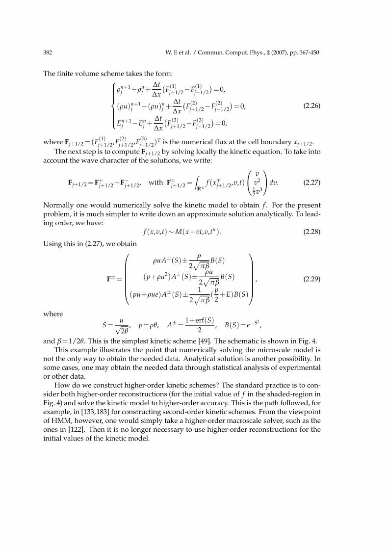
and β=1/2θ. This is the simplest kinetic scheme [49]. The schematic is shown in Fig. 4.This example illustrates the point that numerically solving the microscale model is
not the only way to obtain the needed data. Analytical solution is another possibility. Insome cases, one may obtain the needed data through statistical analysis of experimentalor other data.
How do we construct higher-order kinetic schemes? The standard practice is to con-sider both higher-order reconstructions (for the initial value of f in the shaded-region inFig. 4) and solve the kinetic model to higher-order accuracy. This is the path followed, forexample, in [133,183] for constructing second-order kinetic schemes. From the viewpointof HMM, however, one would simply take a higher-order macroscale solver, such as theones in [122]. Then it is no longer necessary to use higher-order reconstructions for theinitial values of the kinetic model.

W. E et al. / Commun. Comput. Phys., 2 (2007), pp. 367-450 383
t υ υ υ
υ υ υ
υ υ υ∆t
x∆x
Figure 4: Schematics for the derivation of kinetic scheme: A finite volume method is imposed in thex−t domain, and the kinetic equation is solved (e.g. analytically) over the shaded region to give thefluxes needed in the finite volume method. The v axis indicates the extra velocity variable in the kineticmodel, which represents the microstructure for the present problem.
2.2.4 Large scale molecular dynamics (MD) simulation of gas dynamics
In this example we discuss how HMM can be used to carry out macroscale gas-dynamicscalculations using only MD. The macroscopic equations are the usual conservation lawsof density, momentum and energy. In one dimension, it can be expressed in a genericform:
∂tu+∂xf=0. (2.30)
Here f is the flux. Traditional gas dynamics models assume that f is a known function ofu. Here we do not make that assumption. Instead we will extract f from an underlyingatomistic model, namely, molecular dynamics (MD).
As the macroscale solver, we select a finite volume method. One example is the centralscheme of [122] on a staggered grid:
un+1j+1/2 =
unj +un
j+1
2− ∆t
∆x
(fn
j+1−fnj
). (2.31)
The data that need to be estimated from MD are again the fluxes. This is done byperforming a constrained MD simulation locally at the cell boundaries, which are the cellcenters for the previous time step. The constraints are that the average density, momen-tum and energy of the MD system should agree with the local macro state at the currenttime step n. This is realized by initializing the MD with such constraints and apply the

384 W. E et al. / Commun. Comput. Phys., 2 (2007), pp. 367-450
xj xj+1
Uj
Uj
Uj+1
F(Uj )
F(Uj )F(Uj+1 )
Uj+1/2
MD
Figure 5: Central scheme: starting with piecewise constant solution, one computes fluxes at xj and xj+1, andintegrates the conservation laws to the next time step, where the grid points are shifted to the midpoints xj+1/2.The numerical fluxes are evaluated with the help of MD.
periodic boundary condition afterwards. Using the Irving-Kirkwood formula (see Sec-tion 4) which relates the fluxes to the MD data, we can then extract the macroscale fluxesby time averaging the MD data. Ensemble averaging may also be used. We refer to [108]for more details.
One result from such a method is shown in Fig. 6. Here the set-up for the macroscalemodel is a Riemann problem for one-dimensional wave propagation in solids. The mi-croscale model is two-dimensional MD with Lennard-Jone potential. The result of HMMis compared with that of a direct MD simulation.
2.3 A type A example: Coupled kinetic-hydrodynamic simulation of shockpropagation
Our next example is continuum gas dynamics locally corrected near shocks by the kineticmodel. This is a type A problem. Problems of this type have been studied for a long timein the kinetic theory community using domain decomposition methods (see for exam-ple [22, 104]). The framework of HMM suggests a way of handling this problem that isslightly different from what is done in the literature.
The macroscopic process is gas dynamics, the microscopic process is described bya kinetic model. Therefore, as the macroscale solver, it is natural to choose the kineticschemes for gas dynamics. Away from shocks, the numerical fluxes are computed using(2.29). At the shocks the numerical fluxes are computed by solving locally the kineticmodel using micro time steps. The kinetic model is constrained by the local macroscopicstate through the boundary conditions. As shown in Fig. 7, the kinetic equation is solvedin the shaded region between xl and xr (assume that the shock is at the cell boundaryxk+1/2). Boundary condition is needed at xl for v>0. For this we choose
f (xl ,v,t)= M(xl ,v,t), v>0, (2.32)

W. E et al. / Commun. Comput. Phys., 2 (2007), pp. 367-450 385
−1 −0.8 −0.6 −0.4 −0.2 0 0.2 0.4 0.6 0.8 1−15
−10
−5
0
5x 10⁻³
−1 −0.8 −0.6 −0.4 −0.2 0 0.2 0.4 0.6 0.8 1−0.1
−0.05
0
0.05
0.1
0.15
0.2
0.25
0.3
−1 −0.8 −0.6 −0.4 −0.2 0 0.2 0.4 0.6 0.8 1−0.012
−0.01
−0.008
−0.006
−0.004
−0.002
0
Figure 6: Numerical test on shock formation and propagation in solids. 200 macro-grid points are used and eachlocal MD simulation consists of 40×10 atoms and 104 steps of time integration. The solution is displayed after40 steps of integration over macro time steps. Solid line: computed solution; dashed line: full atom simulation(one realization). Top: strain; middle: velocity; bottom: displacement.
where the right-hand side is the local Maxwellian corresponding to the macroscopic stateat xl , obtained by extrapolating the macro states in the cells to the left of xl. Boundarycondition at xr can be handled similarly. At xk+1/2, we define
Fk+1/2 =1
τ
∫ tn+τ
tndt∫
R+f (x−k+1/2,v,t)
vv2
12 v3
dv+
∫
R−f (x+
k+1/2,v,t)
vv2
12 v3
dv
, (2.33)
for suitably chosen τ.How do we choose τ? To address this question, we should note that there are po-
tentially two different cases of interest concerning corrections to gas-dynamics models ofshocks. The first is when non-equilibrium effects are important. In this case the relaxationtime of the gas inside the shock may become comparable to the hydrodynamic time, andwe should simply choose τ = ∆t. Note that in this case there is no time scale separation,and the kinetic model is solved continuously throughout the shock region, with occa-sional re-initialization as the shock region moves. This is shown schematically in the left
386 W. E et al. / Commun. Comput. Phys., 2 (2007), pp. 367-450
t
xxl xr
t
x
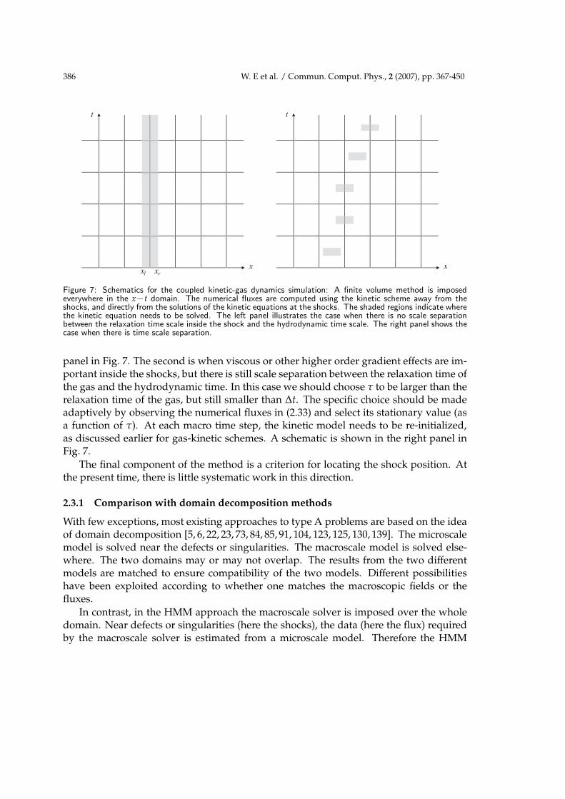
Figure 7: Schematics for the coupled kinetic-gas dynamics simulation: A finite volume method is imposedeverywhere in the x−t domain. The numerical fluxes are computed using the kinetic scheme away from theshocks, and directly from the solutions of the kinetic equations at the shocks. The shaded regions indicate wherethe kinetic equation needs to be solved. The left panel illustrates the case when there is no scale separationbetween the relaxation time scale inside the shock and the hydrodynamic time scale. The right panel shows thecase when there is time scale separation.
panel in Fig. 7. The second is when viscous or other higher order gradient effects are im-portant inside the shocks, but there is still scale separation between the relaxation time ofthe gas and the hydrodynamic time. In this case we should choose τ to be larger than therelaxation time of the gas, but still smaller than ∆t. The specific choice should be madeadaptively by observing the numerical fluxes in (2.33) and select its stationary value (asa function of τ). At each macro time step, the kinetic model needs to be re-initialized,as discussed earlier for gas-kinetic schemes. A schematic is shown in the right panel inFig. 7.
The final component of the method is a criterion for locating the shock position. Atthe present time, there is little systematic work in this direction.
2.3.1 Comparison with domain decomposition methods
With few exceptions, most existing approaches to type A problems are based on the ideaof domain decomposition [5, 6, 22, 23, 73, 84, 85, 91, 104, 123, 125, 130, 139]. The microscalemodel is solved near the defects or singularities. The macroscale model is solved else-where. The two domains may or may not overlap. The results from the two differentmodels are matched to ensure compatibility of the two models. Different possibilitieshave been exploited according to whether one matches the macroscopic fields or thefluxes.
In contrast, in the HMM approach the macroscale solver is imposed over the wholedomain. Near defects or singularities (here the shocks), the data (here the flux) requiredby the macroscale solver is estimated from a microscale model. Therefore the HMM

W. E et al. / Commun. Comput. Phys., 2 (2007), pp. 367-450 387
methodology is closer to that of (adaptive) model refinement [76, 126]: Near defects orsingularities, a more refined model is used to supply the data.
For the example discussed above, the model is adaptively refined at the shocks andis replaced by the kinetic model for flux evaluation. The overall algorithm is still thatof a finite volume method. The kinetic model is used inside the finite volume schemeto provide part of the data. In addition, HMM provides ways of further limiting thesize of the computational domain for the microscopic model, by exploiting time scaleseparation so that the kinetic equation does not have to be solved for all time, or spatialscale separation so that the kinetic equation is solved only in a very thin strip insidethe macro cells. This philosophy is opposite to that of over-lapping – it might be called“under-lapping”. See Fig. 7.
2.4 The fiber bundle viewpoint
It is worth pointing out that when extracting the needed data from microscopic models,one can think of the microscale model as been solved on a “virtual domain”: It is not nec-essary to think of this domain as being part of the physical domain we are interested in.The conceptual framework of HMM is very similar to that of fiber bundles: The physicaldomain is the base manifold, the local microstructures are defined over the fibers. Themapping from the fibers to the base manifold via the compression operator is a local op-eration. This is a key conceptual difference between HMM and domain decompositionor the adaptive model refinement methods. The latter two approaches make explicit useof the fact that both the macro and micro models are defined on the same domain.
The algorithmic consequence of this concept is that under the framework of HMM,the microscale computations carried out over different macroscopic locations communi-cate with each other only through the macroscale solver. By thinking of the microstruc-ture as been defined in a virtual space, we are naturally led to numerical algorithmswhich are free of the limitations associated with filling up the macroscopic space andtime by the microscale grid points and time steps, and this is the reason why HMM en-ables us to design numerical algorithms that are much more efficient than the brute forcemicroscale solvers.
Since HMM relies on a local connection between the microstructures and the macrostate, one might suspect that it is not as effective for problems with long range interac-tions. At the present time, this issue remains to be addressed.
2.5 Recovering information about the microscale process
HMM is designed to capture the macroscale behavior of the underlying system. How-ever, in many cases, particularly for type A problems, we are also interested in someaspects of the microscopic behavior. Possibilities exist within the HMM framework to re-cover such information. The microscale solutions obtained in the data extraction processdo provide samples for the local microstructure.

388 W. E et al. / Commun. Comput. Phys., 2 (2007), pp. 367-450
In this connection, two questions remain to be answered. The first is the accuracy ofsuch microscale information. The second is the sense in which we speak about accuracy.This is a general question in multiscale, multi-physics modeling. In many cases, we canonly expect to capture some statistical or qualitative aspects of the microscopic process.At the present time, this problem has not been formulated in precise terms. We will comeback to such issues later on when we discuss other applications.
3 The heterogeneous multiscale finite element method
Consider
−∇·(kε(x)∇uε(x))= f (x), x∈Ω⊂Rd. (3.1)
Here ε is a small parameter that signifies explicitly the multi-scale nature of the coefficientkε(x), which will be referred to as the conductivity tensor. Problems of this type have beenextensively studied in the context of heat or electric conduction in composite materials,mechanical deformation of composites, etc [18]. In particular, the homogenization tech-nique was initially developed for analyzing these problems [12, 13, 18]. However, exceptfor the case when the microstructure is locally periodic, it is difficult to make use of thehomogenized equations for numerical purpose. In addition, the homogenized equationlacks information about the micro-scale behavior which is important for analyzing stressdistribution in composites, for example.
3.1 The macro-scale solver and the needed data
We will take a finite element approach. For (3.1), the macro-scale solver can be chosensimply as the standard C0 piecewise linear finite element method over a macroscopictriangulation TH of mesh size H. We will denote by XH the macroscopic finite elementspace which could be the standard piecewise linear finite elements over TH.
The data that need to be estimated from the microscale model is the stiffness matrixon TH: A=(Aij), where
Aij =∫
Ω∇Φi(x)KH(x)∇Φj(x)dx. (3.2)
Here KH(x) is the effective conductivity tensor at scale H and Φi(x) are the basis func-tions for XH. Had we known KH(x), we could have evaluated Aij simply by numericalquadrature: Let fij(x)=∇Φi(x)KH(x)∇Φj(x), then
Aij =∫
Ωfij(x)dx≃ ∑
T∈TH
|T| ∑xk∈T
ωk fij(xk), (3.3)
where xk and ωk are the quadrature points and weights respectively, |T| is the vol-ume of the element |T|.

W. E et al. / Commun. Comput. Phys., 2 (2007), pp. 367-450 389
K
Figure 8: Illustration of HMM for solving (3.1). The dots are the quadrature points in (3.3). The little squaresare the microcell Iδ(xk).
In the absence of explicit knowledge of KH(x), our problem reduces to the approxi-mation of the values of KH(xk). This will be done by solving the original microscalemodel locally around each quadrature point xk (See Fig. 8).
Let Iδ(xk)∋xk be a cube of size δ. Consider
−∇·(kε(x)∇φε
)=0, x∈ Iδ(xk). (3.4)
The main objective is to probe efficiently the microscale behavior under the constraintthat the average (e.g. macroscale) gradient of the solution φε is fixed to be a given constantvector. Having solutions to this local problem, we can define the effective conductivitytensor at xk by the relation
〈kε(x)∇φε〉Iδ=KH(xk)〈∇φε〉Iδ
, (3.5)
where 〈v〉Iδ=(1/|Iδ|)
∫Iδ
v(x)dx. The basis of this procedure is the homogenization theo-rem which has been proved in various contexts; the most general result is found in [129].The homogenization theorems allow us to define the effective (or homogenized) conduc-tivity tensor, by considering the infinite volume limit of the solutions of the microscaleproblem subject to the constraint that the average gradient remains fixed. The effectivetensor is defined by an average relation of the type (3.5) in the infinite volume limit, i.e.
L=δ
ε→∞.
In the special case when the microstructure is periodic, the infinite volume problem re-duces to a periodic problem and therefore can be considered on its period.
In practice, one solves (3.4) with the constraint 〈∇φε〉Iδ=e1,··· ,ed respectively, where
d is the spatial dimension of the problem. Denote these solutions by φεj , j=1,··· ,d. Then
(〈kε(x)∇φε1〉Iδ
,··· ,〈kε(x)∇φεd〉Iδ
)=KH(xk). (3.6)
In summary, the overall algorithm consists of the following steps:
390 W. E et al. / Commun. Comput. Phys., 2 (2007), pp. 367-450
• Solve for φε1,··· ,φε
d using the boundary conditions discussed below, at each xk.• Obtain the approximate values of KH(xk) by averaging the microscale solutions
using (3.6).
• Assemble the effective stiffness matrix using (3.3).• Solve the macroscale finite element equation using the effective stiffness matrix. If
we express the macroscale solution in XH in the form of UH(x) = ∑UjΦj(x), thenthe macroscale finite element equation takes the standard form:
AU = F, (3.7)
where U =(U1,··· ,UN)T, F=(F1,··· ,FN)T, and Fj =( f (x),Φj(x)).
The numerical solution UH obtained through this procedure contains informationabout the average behavior of uε itself, but not its gradient. There is potentially an addi-tional important step, which is to obtain information about the gradient of the solution,either through some post-processing techniques or by analyzing the solutions of the mi-croscale problems φε. However, the details of this last step remains poorly understood.We will come back to this point later.
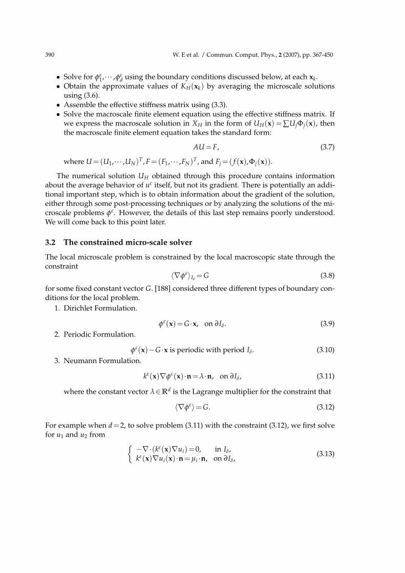
3.2 The constrained micro-scale solver
The local microscale problem is constrained by the local macroscopic state through theconstraint
〈∇φε〉Iδ=G (3.8)
for some fixed constant vector G. [188] considered three different types of boundary con-ditions for the local problem.
1. Dirichlet Formulation.
φε(x)=G ·x, on ∂Iδ. (3.9)
2. Periodic Formulation.
φε(x)−G ·x is periodic with period Iδ. (3.10)
3. Neumann Formulation.
kε(x)∇φε(x)·n=λ·n, on ∂Iδ, (3.11)
where the constant vector λ∈Rd is the Lagrange multiplier for the constraint that
〈∇φε〉=G. (3.12)
For example when d=2, to solve problem (3.11) with the constraint (3.12), we first solvefor u1 and u2 from
−∇·(kε(x)∇ui)=0, in Iδ,kε(x)∇ui(x)·n=µi ·n, on ∂Iδ,
(3.13)

W. E et al. / Commun. Comput. Phys., 2 (2007), pp. 367-450 391
for i=1,2, where µ1 =(1,0)T , µ2 =(0,1)T. Then given an arbitrary G, the Lagrange multi-plier λ=(λ1,λ2)T is determined by the linear equations
λ1〈∇u1〉+λ2〈∇u2〉=G (3.14)
and the solution of (3.11)-(3.12) is given by φε =λ1u1+λ2u2.One can check easily that 〈∇φε(x)〉=G holds for all three formulations.The performance of these formulations was carefully studied in [188]. The main con-
clusions were:
1. Periodic boundary condition performs better than the other two formulations.
2. The variance of the estimated effective tensor behaves as σ2 ∼ L−d for the randomchecker-board problem, and σ2 ∼ L−2 for the periodic problem.
3. In general Neumann formulation underestimates the effective tensor and Dirich-let formulation overestimates the effective tensor. In both cases, the effective con-ductivity tensors converge to the infinite volume limit with first order accuracyO(1/L), where L is the cell size.
This method is extended in [186] to study the elastic deformation of functionallygraded materials.
HMM in this case resembles the idea of representative volume averaging that is com-monly used in subsurface flow modeling, with Iδ playing the role of the representativevolume. In representative volume averaging, the microstructural information is usuallydiscarded after the effective conductivities are extracted out. This is unsatisfactory sincethe microstructural information is particularly important in this case – it contains infor-mation about stress distribution in composite materials or velocity fields in porous media.The HMM philosophy puts more emphasis on the interaction between the macro and mi-croscale behavior. For example, the solutions of the microscale problem (3.5) do containuseful information about the gradients of the solution uε. However, at the present time,very little systematic work has been done on how such information can be extracted,except for the simple case when the microstructure is periodic.
3.3 Other multiscale finite element methods
An alternative proposal for constructing multiscale finite element methods is to modifythe basis functions in the finite element space by solving, for each element, the orig-inal microscale problem with vanishing right-hand side and suitable boundary condi-tions [13–16, 88, 112]. The modified basis functions are used to constructive the effectivestiffness matrix on the coarse grid. This idea was first introduced by Babuska et al. [14]in the context generalized finite element methods for solving elliptic equations with generalrough coefficients. For problems with multiscale coefficients, Hou et al. [88] introducedoverlapping in order to alleviate the difficulties with local boundary conditions. Some

392 W. E et al. / Commun. Comput. Phys., 2 (2007), pp. 367-450
rudimentary versions of this idea was also suggested in [112] for solving Helmholtz equa-tions by using oscillatory functions as basis functions.
Once the basis functions and the effective stiffness matrix is computed, the modifiedbasis function method works efficiently as a coarse grid method. The main problem,however, is in the overhead for computing the basis functions. This overhead is alreadycomparable with solving the original microscopic problem, if a linear scaling methodsuch as multi-grid is used. As all other upscaling methods, the goal of both HMM-FEMand the modified basis function method is to obtain the effective stiffness matrix at themacroscale. The difference lies in how this goal is achieved. HMM-FEM approximatesthe stiffness matrix directly by performing local simulations of the original microscalemodel. The size of the local simulation can be chosen according to the special features ofthe problem. In particular, one may choose the domains of the local problems such thatthey overlap with each other and their union covers the whole computational domain.This would make HMM-FEM very close to the modified basis function methods, andmost likely also defeat the purpose of HMM-FEM. The modified basis function methodobtains the effective stiffness matrix by going through an intermediate step, namely mod-ifying the basis functions and as a result, the original finite element space. This limits itsflexibility in exploring the multiscale features of the underlying problem. Indeed, withthe modified basis function method, solving a problem with structure is as hard as solvinga problem without structure. On the other hand, these techniques might be of some useif the problem (2.17) is solved repeatedly with different right hand side, in which casethey can be used as pre-processing techniques, in the same way as LU decomposition,computation of Schur complements [68], and sub-structuring methods [24].
For a more detailed discussion of these methods and their relative performance, werefer to [119]. It was found, among other things, that the accuracies of HMM-FEM andthe modified basis function method are generally comparable, despite the difference incost.
For the special case when the microstructure of aε is locally periodic, several othermethods have been proposed. Some are based on solving the homogenized equations,plus next order terms [44]. One interesting idea, proposed by Schwab et al. [157, 158],uses multiscale test functions. In this case, the finite element space has a tensor productstructure, which can be exploited to compensate for the increased dimensionality causedby using the multiscale test functions.
4 Complex fluids and microfluidics
The behavior of liquids is usually very well described by the classical Navier-Stokesequations with the no-slip boundary condition. There are two notable exceptions. Thefirst is non-Newtonian fluids such as polymeric fluids. In this case the constitutive equa-tions are more complex than that of Newtonian fluids, for which the viscous stress issimply a linear function of the rate of strain. The second is micro-fluidics. In this case the
W. E et al. / Commun. Comput. Phys., 2 (2007), pp. 367-450 393
geometry of the flow domain is so small that the no-slip boundary condition is no longeraccurate enough.
Three different levels of models are commonly used in the modeling of liquids: molec-ular dynamics, Brownian dynamics, and hydrodynamics. We will discuss the case whenthe microscale model is molecular dynamics and the macroscale model is hydrodynam-ics. But some of the issues that we will discuss are also relevant if the microscale modelis Brownian dynamics. For simplicity we will assume that the flow is incompressible.Extending the methodology to compressible flows is quite straightforward. This sectionis taken mostly from [146].
4.1 The macroscale and microscale models
At the continuum level, the dynamics of incompressible flow has to obey conservationlaws of mass and momentum:
ρ∂tu=∇·τ,∇·u=0,
(4.1)
where the momentum flux −τ = ρu⊗u−τd. Here ρ is the density of the fluid which isassumed to be a constant, u=(u,v) is the velocity field, and τd is the stress tensor. We willlimit ourselves to the situation when the flow is macroscopically two-dimensional (mi-croscopically it is of course three-dimensional). But extension to macroscopically three-dimensional flows is straightforward. At this stage the system is not closed since thestress tensor is yet to be specified. Traditionally the idea has been to close this system byan empirically postulated constitutive relation, such as
τd =−pI+µ(∇u+∇uT) (4.2)
for simple fluids. In this case, all information about the molecular structure is lumpedinto one number, the viscosity µ. Here we are interested in the situation when empir-ical constitutive relations are no longer accurate enough, and more information at themicroscopic level is needed.
Another important component in the model is the boundary condition. Almost allmacroscopic models assume the no-slip boundary condition
u=u0, (4.3)
where u0 is the velocity of the boundary. This is adequate in many situations, but be-comes questionable for some problems in micro-fluidics.
For the microscopic model, we will use molecular dynamics (MD). Using standardnotations for liquids, we have
mixi(t)=pi(t),pi(t)=Fi,
(4.4)
i=1,2,··· ,N. Here mi is the mass of the i-th particle, xi and pi are its position and momen-tum respectively, Fi is the force acting on the i-th particle. To examine the behavior of the

394 W. E et al. / Commun. Comput. Phys., 2 (2007), pp. 367-450
fluid flow near a solid boundary, we should also model the vibration of the atoms in thesolid next to the fluid-solid interface. Therefore one should consider the fluid-solid sys-tem as a whole. We will work in the isothermal setting, and the Nose-Hoover thermostatcan be used to control the temperature of the system [75].
The connection between the atomistic and the continuum models is made as follows.Given the microscopic state of the system xi(t),pi(t)i=1,2,···,N , we define the empiricalmomentum distribution
m(x,t)=∑i
pi(t)δ(xi(t)−x), (4.5)
where δ is the Delta function. Momentum conservation can then be expressed in termsof the microscopic variables as:
∂tm=∇·τ(x,t), (4.6)
where the momentum current density τ(x,t) is given by the following Irving-Kirkwoodformula [90]:
τ(x,t)=−∑i
1
mi(pi(t)⊗pi(t))δ(xi(t)−x) (4.7)
− 1
2∑j 6=i
((xi(t)−xj(t))⊗Fij(t)
)∫ 1
0δ(λxi(t)+(1−λ)xj(t)−x)dλ,
where Fij(t) is the force acting on the i-th particle by the j-th particle.An important issue in molecular dynamics is how to model the atomistic forces ac-
curately. The algorithms that we will discuss are quite insensitive to the details of theatomistic potential. For simplicity we will work with the simplest situation when theinteraction between particles is pair-wise and the pair potential is the Lennard-Jones (LJ)potential in a slightly modified form:
VLJ(r)=4ε
((σ
r
)12−η(σ
r
)6)
. (4.8)
Here r is the distance between the particles, ε and σ are characteristic energy and lengthscales respectively. The parameter η controls the nature of the interaction between parti-cles. When η =1, (4.8) defines the usual LJ potential which is attractive at long distance.Repulsion between particles of different species can be modeled using negative values ofη.
It proves convenient to use the reduced atomic units. The unit of length is σ. The unitof time is σ
√m/ε. For temperature it is ε/kB where kB is the Boltzmann constant, and for
density it is m/σ3. The unit of viscosity is (εm)1/2/σ2. The unit of surface tension is ε/σ2.
4.2 Type B problems: Atomistic-based constitutive modeling
4.2.1 Macroscale solver
As the macroscopic solver, we choose the projection method on a staggered grid [39, 40].The projection method is a fractional step method. At each time step, we first discretize

W. E et al. / Commun. Comput. Phys., 2 (2007), pp. 367-450 395
Figure 9: Schematic of the spatial discretization of the continuum equations in (4.1). u is defined at (xi,yj+ 12),
v is defined at (xi+ 12,yj), and p is at the cell center (xi+ 1
2,yj+ 1
2). τ11 and τ22 are calculated at the cell center
indicated by circles, and τ12 is calculated at the grid points indicated by squares.
the time derivative in the momentum equation by the forward Euler scheme to obtain anintermediate velocity field:
ρun+1−un
∆t=∇·τn, (4.9)
where τn is the momentum flux. For the moment, pressure as well as the incompressibil-ity condition are neglected. Next the velocity field un+1 is projected onto the divergence-free subspace:
ρun+1−un+1
∆t+∇pn+1 =0, (4.10)
where pn+1 is determined by
∆pn+1 =ρ
∆t∇·un+1, (4.11)
usually with Neumann boundary condition.
The spatial discretization is shown in Fig. 9. For integer values of i and j, we define uat (xi,yj+1/2), v at (xi+1/2,yj), and p at the cell center (xi+1/2,yj+1/2). The diagonals of theflux τ are defined at (xi+1/2,yj+1/2), and the off-diagonals are defined at (xi,yj). The op-erators ∇ and ∆ are discretized by standard central difference and the five-point formularespectively. The use of this grid simplifies the coupling with molecular dynamics.
4.2.2 Estimating the stress
The data that need to be estimated from molecular dynamics are the stresses. Here wewill make a constitutive assumption, namely that the stress depends only on the rateof strain. We do not need to know anything about the specific functional form of thisdependence.
The key component in estimating the stress is to construct a constant rate-of-strainensemble for the MD. This is done through a modified periodic boundary condition.

396 W. E et al. / Commun. Comput. Phys., 2 (2007), pp. 367-450
4.2.3 Constrained microscopic solver: Constant rate-of-strain MD
There exists an earlier work due to Lees and Edwards [103] in which the periodic bound-ary condition is modified to maintain a constant shear in one direction. This is done byshifting the periodic copies of the simulation box above and below in opposite directionsaccording to the given shear profile. This idea was extended to situations with generallinear velocity profiles in [146].
Without loss of generality, we will consider the situation when the macroscopic ve-locity profile is of the form
uvw
=
a b 0c −a 00 0 0
xyz
= Ax. (4.12)
To initialize the MD calculation, one may simply start with a perfect lattice configurationin a rectangular box. Each particle is given a mean velocity according to (4.12), plus arandom component with mean 0 and variance kBT, where T is the desired temperatureand kB is the Boltzmann constant.
Deforming the simulation box. Periodic boundary condition is imposed on a dynami-cally deforming simulation box, whose vertices move according to
x= Ax, A=
a b 0c −a 00 0 0
. (4.13)
Intuitively it is helpful to think of the simulation box as been embedded in the wholespace.
The shape of the deformed box at a later time is shown in Fig. 10(b). Suppose at thispoint a particle crosses the boundary at P(x), with velocity u, it will return to the box atP′(x′) with a modified velocity
u′=u+A(x′−x), (4.14)
where P′ is the periodic image of P with respect to the deformed box.
It is easy to see that if the velocity field is a pure shear
A=
0 b 00 0 00 0 0
, (4.15)
then this boundary condition becomes simply the Lees-Edwards boundary condition.
Re-initialization. As the simulation proceeds, the simulation box will in general becomequite elongated in one direction and narrowed in the other direction (see Fig. 10(c)). If

W. E et al. / Commun. Comput. Phys., 2 (2007), pp. 367-450 397
the box is significantly deformed, we need to re-initialize the configuration. An approx-imate re-initialization procedure is discussed in [146]. A more accurate re-initializationprocedure that makes use of reproducing lattice is discussed in [147].
The MD simulation keeps track of the positions and velocities of all particles as func-tions of time, from which the instantaneous momentum flux tensor can be calculatedusing the Irving-Kirkwood formula (4.7).
In practice, (4.7) is averaged over the simulation box. This gives
−τ(t)=1
|Ω| ∑xi∈Ω(t)
1
mi(pi⊗pi)+
1
2|Ω|∑j 6=i
dij(xi−xj)⊗Fij, (4.16)
where in the first term the summation runs over particles inside the box, and in the sec-ond term the summation is over all pairs of particles including their images. Here dij isdefined as
dij =
1, if xi,xj ∈Ω,0, if xi,xj /∈Ω,c, if only one of xi,xj is in Ω,
(4.17)
where 0≤ c≤ 1 is the fraction of |xi−xj| being cut by the box. Therefore besides contri-butions from the particles inside the box, particles outside the box also contribute to thestress, as illustrated in Fig. 11.
Eq. (4.16) gives the instantaneous stress at the microscopic time t (see Fig. 12). Toextract the macroscopic stress, (4.16) is averaged over time to give an estimate for themacroscale stress:
τ =1
T−T0
∫ T
T0
τ(t)dt, (4.18)
where T0 is some relaxation time.
In Fig. 12, we show two numerical examples of the calculated stress. In atomic unitsthe density is ρ = 0.79 and the temperature is fixed at 1.0 in the first example but not inthe second which is not coupled to any thermostats. The stress diverges in this case dueto viscous heating.
As a simple validation of this procedure, we show in Fig. 13 the computed shearstress as a function of shear rate for LJ fluids. These data fit quite well to a linear functionindicating a linear relation between stress and the rate of strain. The viscosity can becomputed by estimating the slope. This gives a value of 2 which agrees well with resultsin the literature [171].
To summarize, at each macro time step k, the overall algorithm looks as follows:
Step 1 Calculate the needed stresses by constrained local MD simulations;
Step 2 Using the projection method and the computed stresses to get uk+1.
398 W. E et al. / Commun. Comput. Phys., 2 (2007), pp. 367-450
(a)
P
P’
(b) (c)
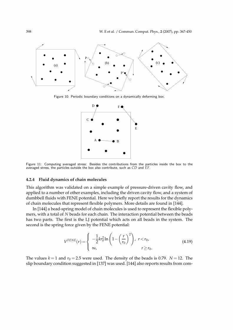
Figure 10: Periodic boundary conditions on a dynamically deforming box.
A B
C
D F
E
Figure 11: Computing averaged stress: Besides the contributions from the particles inside the box to theaveraged stress, the particles outside the box also contribute, such as CD and EF.
4.2.4 Fluid dynamics of chain molecules
This algorithm was validated on a simple example of pressure-driven cavity flow, andapplied to a number of other examples, including the driven cavity flow, and a system ofdumbbell fluids with FENE potential. Here we briefly report the results for the dynamicsof chain molecules that represent flexible polymers. More details are found in [144].
In [144] a bead-spring model of chain molecules is used to represent the flexible poly-mers, with a total of N beads for each chain. The interaction potential between the beadshas two parts. The first is the LJ potential which acts on all beads in the system. Thesecond is the spring force given by the FENE potential:
VFENE(r)=
−1
2kr2
0 ln
(1−(
r
r0
)2)
, r< r0,
∞, r≥ r0.
(4.19)
The values k = 1 and r0 = 2.5 were used. The density of the beads is 0.79. N = 12. Theslip boundary condition suggested in [137] was used. [144] also reports results from com-

W. E et al. / Commun. Comput. Phys., 2 (2007), pp. 367-450 399
0 200 400 600 800 1000−8
−6
−4
−2
0
2
4
(a)
0 200 400 600 800 1000
−10
−8
−6
−4
−2
0
2 (b)
Figure 12: Instantaneous stress as a function of the microscopic time. Solid line: −τ12; dashed line: −τ11;dotted line : −τ22. The temperature is fixed in (a) but not in (b), where the stress diverges due to viscousheating. In both case, u=0.18y, v=0.
0 0.02 0.04 0.06 0.08 0.10
0.05
0.1
0.15
0.2
Shear rate
She
ar s
tres
s
Figure 13: Shear stress as a function of shear rate for simple LJ fluids. The discrete points are obtained from 3dMD simulation, and they fit very well to a linear function with slope 2 which is the viscosity. All the quantitiesare expressed in the atomic unit.
putations that treat this as a type C problem and extract boundary conditions using thealgorithm described next for type A problems. The results are basically the same.
At small driving force, there is only partial slip between the fluid the solid. The ve-locity profile converges to steady state, as shown in Fig. 14. This steady state profile iscompared with the standard Poiseuille profile at the zero-shear-rate viscosity. Besidesthe partial slip, we also see that the profile for the chain molecules has larger curvature,a characteristic of shear thinning fluids. This is confirmed by the plot of the effectiveconstitutive relation used in the HMM simulation at the steady state.

400 W. E et al. / Commun. Comput. Phys., 2 (2007), pp. 367-450
η=7.5
(a)
5 15 25
5
−5
5
15
25
x
y
z
(b)
0 0.05 0.1 0.15 0.2 0.250
0.1
0.2
0.3
0.4
0.5
0.6
0.7
0.8
Shear rate
τ
(c)
0 0.05 0.1 0.15 0.2 0.253
3.5
4
4.5
5
5.5
6
6.5
7
7.5
Shear rate
η
(d)
Figure 14: (a): Steady state velocity profile for the polymer fluid made up of chain molecules (solid line),compared with that of the Newtonian fluid (dashed line). We observe partial slip, as well as shear-thinning.(b): A partial sample of the conformation of the chain molecules in a typical MD simulation. (c): Shear stressas a function of shear rate. (d): Viscosity as a function of shear rate. In (c) and (d), to make the resultsmore transparent, we supplemented the results from the HMM calculation by results from pre-computing: Themore noisy results at small shear rates are from HMM calculation, the smoother results at higher shear ratesare obtained via pre-computing.
4.3 Type A problems: Modeling boundary conditions
In the discussions above we were concerned with the constitutive relations for complexfluids. Here we will discuss boundary conditions for micro-fluidics. One most importantaspect of micro-fluidics is the significance of line and surface tension. Therefore as ourprimary examples, we choose the Marangoni flow and the contact line problem. Forthese problems, the need for coupling with MD comes from the complex fluid-solid andfluid-fluid interaction near the wall.
4.3.1 Marangoni flows
We will discuss a specific example of the Marangoni flow, namely channel flow drivenby complex solid-fluid interactions which are modeled by molecular dynamics.
The HMM procedure goes as follows. The macroscopic solver is the same as before,i.e. a finite-volume projection method on a staggered grid. This simplifies the next step,which is to obtain the boundary condition from MD.

W. E et al. / Commun. Comput. Phys., 2 (2007), pp. 367-450 401
x
A
F
B
E H G
BA
Repulsive Force
Sampling Region
z
y D C Constrained MD
D C
Figure 15: Schematic of the multiscale method for the example of Marangoni flow. In the left panel, thefinite volume grid is indicated by the dotted lines. The boundary condition at AB is extracted from moleculardynamics simulations confined in ABCD. The set-up of the MD simulation is shown in the right panel. Particlesare confined by a repulsive force at GH and the solid wall at AB. The dynamics of the particles in the strip CDare constrained by the continuum velocity field. The boundary conditions are extracted from the small bins atthe lower boundary. Black dots represent atoms in the solid.
The needed data in the finite volume projection method are the tangential stresses atthe boundary.
The schematic of the MD is shown in Fig. 15. Periodic boundary condition is imposedin the x- and z-direction. In the y-direction, the fluid is confined by a solid wall at AB anda repulsive force at GH. One choice of this repulsive potential is the repulsive part of theLJ potential:
P(r)= ε(σ
r
)12, (4.20)
where r is the distance to GH. Similar techniques for confining particles were used in[84, 85].
The MD is constrained by the macroscale velocity field. This is done as follows.Each particle in the strip CD is assigned the velocity: u(x) = uc(x)+u, where uc(x) isthe velocity from the continuum calculation and u is the thermal velocity that obeys theMaxwellian distribution at some temperature T. Therefore the strip plays a two-fold rolehere: As a momentum reservoir it maintains the non-equilibrium dynamics at the steadystate; as a thermal reservoir it releases heat generated by viscous flow from the system.
The solid wall also needs to be explicitly modeled, here as a crystal lattice. Geometricas well as chemical heterogeneities can be modeled by choosing appropriate atomisticpotentials (see [140, 146]).
After a relatively short equilibration time, the stresses are estimated using the Irving-Kirkwood formula, as was done before.
Fig. 16 shows some results of the effective boundary conditions extracted from themolecular dynamics simulation. For more numerical results, we refer to [146].
The overall algorithm for a typical macro time step k is as follows:
Step 1 Calculate the stress at the boundary AB by local MD simulation. The MD is con-strained by uk;

402 W. E et al. / Commun. Comput. Phys., 2 (2007), pp. 367-450
0 0.4 0.8 1.2 1.6 20.02
0.06
0.1
0.14
2 x / L
u(x
,y=
0)
(a)
0 0.4 0.8 1.2 1.6 2−0.01
0
0.01
0.02
0.03
0.04
2 x / L
Sh
ea
r S
tre
ss
(b)
Figure 16: (a): the velocity at the lower boundary; (b): the stress extracted from MD (solid curve) and fittedby fourth-order B-splines (dashed curve).
Step 2 Solve the continuum equations to get uk+1.
4.3.2 Contact line dynamics
We next consider the motion of two immiscible fluids on a solid surface. Continuumhydrodynamics breaks down in the vicinity of the contact line, where the fluid-fluid in-terface meets the solid surface. Specifically the usual no-slip boundary condition used inmacroscopic fluid dynamics leads to an unphysical divergent shear stress and dissipationrate [52]. Molecular dynamics simulations of Couette or Poiseuille flow show relative slipbetween the fluid and the wall around the contact line [141, 171].
As for the previous example, a HMM procedure is called for in order to obtain bound-ary conditions from MD. However the present problem is quite a bit more complicated.
Macroscale solver
As the macroscale model, we take
ρ∂tu=∇·τ,∇·u=0,xΓ =u,
(4.21)
where the momentum flux in continuum theory is given by
−τ =ρu⊗u+pI−µ(∇u+∇uT)+γ(I−n⊗n)δΓ− f0xI. (4.22)
The last equation in (4.21) says that the fluid-fluid interface xΓ(t) is advected by the ve-locity field of the fluid. The first term in the momentum flux is due to convection, thesecond term is the pressure, the third term is the viscous stress, the fourth term corre-sponds to the surface tension force which is concentrated at the fluid-fluid interface xΓ

W. E et al. / Commun. Comput. Phys., 2 (2007), pp. 367-450 403
(δΓ is the surface delta function), and the last term is the external force. I is the identitymatrix, γ is the the surface tension coefficient and n is the unit normal of the interface.
In the numerical calculations, it is standard to replace the surface tension term τΓ =γ(I−n⊗n)δΓ as a body force defined by
τΓ(x)=∫
R2D(x−y)τΓ(y)dy. (4.23)
One choice for the kernel D is given by
D(x)=
(2d)−2(1+cos(πx/d))(1+cos(πy/d)), if |x|<d, |y|<d;0, otherwise.
(4.24)
This was first introduced by Peskin [134]. In the examples reported below, d, the widthof the smoothing region, is taken to be twice the cell size. After being interpolated fromthe interface to the grid points by (4.23), the total flux is conserved.
As before we use the projection method for the macroscale equation. The interface isupdated by forward Euler method:
(xΓ)n+1−(xΓ)n
∆t=un. (4.25)
The interface is represented by a collection of discrete points (xΓ)i,i=0,1,··· ,N, wherethe two end points (xΓ)0 and (xΓ)N are the contact points, i.e. the intersections of theinterface with the solid walls. Surface tension force is calculated at the middle of eachsegment. Neumann condition on velocity is used at the in-flow and out-flow boundaries.At the solid wall away from the contact point, no-slip boundary condition is used. Otherdetails of the macroscale solver can be found in [146].
Microscopic solver and estimating boundary conditions
The data that need to be estimated from MD are:
1. shear stress near the contact line (here the contact point);
2. velocity of the contact line.
The schematics of the molecular simulation around the contact line is shown in Fig. 17.Periodic boundary conditions are imposed in the z-direction. In the x-direction, the flowfield is not necessarily periodic, so we enlarge the simulation box to G′H′C′D′ and imposeperiodic boundary conditions on G′D′ and H′C′ instead (see the right panel in Fig. 17).The enlarged part serves as a particle reservoir. In this system we have two species of flu-ids, fluid I on the left and fluid II on the right. When a fluid particle of species II crossesH′C′, it will enter the box through G′D′ and become species I, and vice versa.
In the y-direction, the particles are confined by the solid wall at G′H′ and a repulsiveforce at C′D′. The repulsive force is modeled by the repulsive part of the LJ potential, as

404 W. E et al. / Commun. Comput. Phys., 2 (2007), pp. 367-450
A
F
B
ERepulsive Force
CD
Sampling Region
Constrained MD
G G H H’
C’
θ
z
x
y
Ι ΙΙ
Ι ΙΙ
H
D’
C
G’
DO
Figure 17: Schematic of the multiscale method for the contact line problem. Macro grid used in the computationis represented by dotted lines in the left panel. MD is carried out in a local region around the contact line.Periodic boundary conditions are imposed on the boundaries of the enlarged box G′D′ and H′C′. The dynamicsin the shaded strips GD, DC and CH are constrained by continuum velocity field. The shear stress and theposition of the contact point are computed in the strip along GH.
given in (4.20). The repulsive force is used to keep the particles from escaping the MDdomain. More detailed information on the microscale solver is given in [146].
For consistency between the molecular dynamics and the continuum dynamics, amodified Andersen thermostat is used in the strips GD,DC, and CH: At Poisson dis-tributed times with certain frequency ν, a random particle is selected from the strips andits velocity is replaced by u(x)= uc(x)+u, where uc is the velocity from continuum dy-namics and u is a random variable with Maxwell-Boltzmann distribution at the specifiedtemperature T.
The shear stress is calculated using the formula (4.7) in the bins which are a few (about3) atomic lengths above the wall.
To estimate the position of the contact line, we first calculate the particle density func-tion along the fluid-solid interface (remember O is fixed):
ρ(x)=∑i
ρi δ(xi−x), (4.26)
where the sum is over all particles in the strip above the solid wall, xi is the x coordinateof the i-th particle, ρi is 1 for particles of species I and -1 for particles of species II. Theposition of the contact line is determined by ρ(x)=0. [146] suggests taking a strip which isagain a few atomic lengths above the wall and partition it into uniform bins in x direction.Then the density is obtained by taking the sum of ρi in each bin. The position of thecontact line is given by
(xΓ)0 = x0+∫ x1
x0
ρ(x)dx, (4.27)
where x0 and x1 are the positions of the leftmost and the rightmost bins respectively. ρ(x),which is between 0 and 1, is the rescaled density:
ρ(x)=ρ(x)−minx ρ(x)
maxxρ(x)−minx ρ(x) . (4.28)

W. E et al. / Commun. Comput. Phys., 2 (2007), pp. 367-450 405
Numerical results
The overall algorithm for a typical macro time step k looks like the following:
Step 1 Carry out a constrained MD simulation near the contact line, from which theshear stress and the position of the contact line are estimated;
Step 2 Solve equations in (4.21) for uk+1 and (xΓ)k+1.
We will discuss two examples from [146]. The first example is a validation study. Thesecond is an example of asymmetric fluid-solid interactions.
Example 4.1. Two immiscible fluids are confined in a channel and driven by an externalforce f0=0.02 in the x direction. The system measures 69.7×22.5×5.16 and contains 2944particles of each fluid and 1728 solid particles. The system is periodic in the x and zdirections.
To check the validity of the constrained molecular dynamics used in the hybrid meth-od, a local MD simulation is performed around the contact line. The left panel of Fig. 18shows the time series for the difference of the particle numbers of both species insideGDCH (see Fig. 17). We clearly see a transient time during which the particles of speciesI flow out of the box and particles of species II flow into the box. The right panel ofFig. 18 is a comparison between the shear stress calculated on the surface of the solidwall in the full MD simulation and in the local constrained MD simulation, and we seegood agreements.
The validation study was also carried out for the steady-state solution. The parame-ters in the continuum model are ρ=0.81,µ=2.0 and γ=3.7. 70×20 grid points are usedin the spatial discretization, and the time step is ∆t = 0.05. A static configuration wasused as the initial data and the external force is slowly increased to 0.02. The steady-statevelocity field and the interface (dashed line) are shown in Fig. 19. These results agreewell with the full MD results.
Example 4.2. In our next example, we consider the case for which the fluid-solid inter-action is different for the two fluid phases. Specifically the attraction between fluid I andthe solid is decreased by taking η =0.7 in the potential (4.8). All other parameters in thepotential are kept unchanged from the previous example. The static contact angle θ inthis case is 65.
Again the static configuration is used as the initial state and an external force f0(t)=5.35×10⁻¹¹t in x-direction is applied until it reaches f0 = 2.2×10⁻⁵. The force is thendecreased at the same rate until it reaches f0 =−7.0×10⁻⁵. The fluid-fluid interfaces atdifferent times are shown in Fig. 20(a) . The left-most dashed line is the interface at thestatic position, and it travels in the stream-wise direction as the external force increases.The right-most dashed line corresponds to f0=2.2×10⁻⁵. The solid lines from the right tothe left show the shapes of the interfaces as the external force decreases. Fig. 20(b) showsthe dynamic contact angle as a function of the applied force. Again, the dashed curvecorresponds to the dynamics as the force increases, and the solid curve corresponds tothe dynamics as the force decreases.

406 W. E et al. / Commun. Comput. Phys., 2 (2007), pp. 367-450
0 50 100 150 200 250−600
−500
−400
−300
−200
−100
0
100
time
∆N
(a)
0 0.1 0.2 0.3 0.4 0.50
0.1
0.2
0.3
0.4
0.5
0.6
0.7
0.8
x / L
She
ar s
tres
s
(b)
Figure 18: Results of the constrained MD simulation. (a): The time series of ∆N=NI(t)−NI I(t), where NI(t)and NI I(t) are the particle numbers of the two species in the box GDCH (see Fig. 17) respectively; (b):The shear stress measured at the solid wall. The solid curve is calculated from the full MD simulation and thedashed curve is from the constrained MD simulation.
While the numerical results appear to be quite reasonable and in some cases havebeen validated by direct MD simulations, the coupling procedures, the way in whichconstraints are imposed on the MD, are still quite ad hoc. This is a common problem forcoupled atomistic-continuum modeling of fluids: So far there has been little systematicstudy on the accuracy of such coupling procedures. In comparison, more work has beendone on this issue for solids.
5 Dynamics of solids at finite temperature
Unlike fluids, the multiscale nature of solids is much more pronounced. On the model-ing side, there is no analog of the Navier-Stokes equation as a fundamental macroscopicmodel. On the physics side, solids often contain a hierarchy of structures and defects atdifferent scales [136]. These include point defects such as vacancies and impurities, dis-locations and structures formed by dislocations, grain boundaries, and even cracks. As aresult, multiscale modeling has received more attention in solids than in fluids.
We will again focus our discussion on the situation when the macroscopic model iscontinuum mechanics and the microscopic model is molecular dynamics. For the anal-ysis of static properties of solids at zero temperature, in which case the mathematicalmodels reduce to minimization problems, the quasi-continuum method has had a greatdeal of success [169]. Here we will discuss multiscale methods that handle the dynamicsof solids at finite temperature. This part of the presentation follows mainly [108].

W. E et al. / Commun. Comput. Phys., 2 (2007), pp. 367-450 407
0 0.2 0.4 0.6 0.8 1
0
0.28
x / L
y / L
Figure 19: The steady-state solution of Example 4.1 by the hybrid method and comparison with the resultsof full MD. The interface is shown in dashed curve. The solid curve shows the interface obtained by full MDsimulation.
0
1
2
−4 −3 −2 −1 0 1 2 3
y / L
x / L
(a)
−8 −6 −4 −2 0 250
55
60
65
70
75
80
85
90
f0 / F
Con
tact
Ang
le (
degr
ees)
(b)
Figure 20: Dynamics of the contact line problem with asymmetric fluid-solid interactions. (a): Fluid-fluidinterfaces at different times. For dashed curves from left to right, the external force increases from 0 to2.2×10−5; For solid curves from right to left, the external force decreases from 2.2×10⁻⁵ to −7.0×10⁻⁵; (b):
Dynamic contact angle as a function of external force. The external force is rescaled by F =8.1×10⁻⁶.
5.1 Macroscopic and microscopic models
Again the continuum model is expressed in terms of the conservation laws. For solidsit is more convenient to work with Lagrangian coordinates. Denote by x0 the referencecoordinate for the solid and x=x0 +u(x0,t), the position after deformation, with u beingthe displacement. Then the conservation laws take the form:
∂tA−∇x0 v=0,∂tv−∇x0 ·σ =0,ρ0∂te+∇x0 ·j=0.
(5.1)

408 W. E et al. / Commun. Comput. Phys., 2 (2007), pp. 367-450
Here A,v,e are the deformation gradient, velocity and total energy per particle respec-tively, ρ0 is the initial density, σ is the first Piola-Kirchhoff stress tensor and j is theenergy flux. The first equation in (5.1) is a statement of compatibility between the de-formation gradient and the velocity. The second and third equations are conservation ofmomentum and energy respectively. In continuum mechanics [100], these equations aresupplemented by the empirical constitutive relations for stress and energy fluxes. Ourinterest here is to develop multiscale strategies that bypass these empirical constitutivelaws when their accuracy is in doubt.
The microscopic model is again MD. The first step is to derive a set of conservationlaws similar to (5.1). For this purpose, we define the following empirical distributions[108],
ρ(x0,t)=∑i
miδ(x0−x0i ),
v(x0,t)=∑i
vi(t)δ(x0−x0i ),
q(x0,t)=∑i
mivi(t)δ(x0−x0i ),
e(x0,t)=1
2 ∑i
[mivi(t)2+∑
j 6=i
φ(xi(t)−xj(t)
)]δ(x0−x0
i ).
(5.2)
Here as before we denote by x0i the position of the i-th atom in the undeformed configu-
ration, xi(t) and vi(t) are respectively the position and velocity of the i-th atom at time t.Let
σαβ(x0,t)=−1
2 ∑i 6=j
fα
(xi(t)−xj(t)
)(x0
iβ−x0jβ)
×∫ 1
0δ(x0−(x0
j +λ(x0i −x0
j )))dλ,
j(x0,t)=1
4 ∑i 6=j
(vi(t)+vj(t)
)·f(xj(t)−xi(t)
)(x0
i −x0j )
×∫ 1
0δ(x0−(x0
j +λ(x0i −x0
j )))dλ,
(5.3)
where f =−∇V is the force and we have only considered two-body interaction in theatomistic potential – extension to the general case can be found in [108]. We have
∂tq−∇x0 ·σ =0,
ρ0∂t e+∇x0 · j=0.(5.4)
The expressions in (5.3) are nothing but the generalizations of the classical Irving-Kirkwoodformula.

W. E et al. / Commun. Comput. Phys., 2 (2007), pp. 367-450 409
xk−1
xk x
k+1
tn
tn+1
tn+2
uk−1n u
kn u
k+1n
uk−1/2n+1 u
k+1/2n+1
fk−1n f
kn f
k+1n
fk−1/2n+1 f
k+1/2n+1
[] [] []
[] []
Figure 21: A schematic illustration of the numerical procedure: starting from piece-wise constant solutionswn
k , one integrates (5.5) in time and in the cell [xk,xk+1]. To estimate f at xk, we perform a MD simulationusing wn
k as constraints.
5.2 Type B problem: Atomistic-based constitutive modeling
5.2.1 Macroscale solver
Our basic macroscopic model is a set of conservation laws. Therefore, as the macroscalesolver, we will choose a finite volume method. Although there are a variety of finitevolume methods available for solving conservation laws [80, 105], many of them involvecomputing the Jacobian of the flux functions, which dramatically increases the computa-tional complexity in a coupled multiscale method when the constitutive relation has tobe extracted from atomistic models. An exception is the central scheme of Lax-Friedrichstype, such as the one developed in [122] which is formulated over a staggered-grid. Be-low we will choose such central schemes as our macroscale solver.
For convenience, we will illustrate the case when the macroscale model is one-dimen-sional. We rewrite the conservation laws in a generic form,
wt+fx =0, (5.5)
where w denotes the conserved quantities, and f is some (unknown) flux function. Fig. 21shows the overall structure of the method. The first order central scheme represents thesolutions by piece-wise constants, which are the average values over each cell:
wnk =
1
∆x
∫ xk+1/2
xk−1/2
w(x,tn)dx.

410 W. E et al. / Commun. Comput. Phys., 2 (2007), pp. 367-450
Here ∆x is the size of the cell. Integrating (5.5) over [xk, xk+1]×[tn, tn+1) leads to thefollowing:
wn+1k+1/2 =
wnk +wn
k+1
2− ∆t
∆x
(fn
k+1−fnk
), (5.6)
where
fnk =
1
∆t
∫ tn+1
tnf(xk,t)dt.
This is then approximated using numerical quadrature such as the mid-point formula. Asimple choice is fn
k ∼ f(xk,tn).The overall procedure is as follows. At each macro time step, the scheme (5.6) requires
as input the fluxes at the grid points xk. These flux values are obtained by performinglocal MD simulations that are constrained by the local macro state variables A, v, e. Afterthe MD system equilibrates, we estimate the fluxes by time/ensemble averaging.
Higher-order schemes and generalization to high dimensions are discussed in see[108].
5.2.2 Constrained microscale solver
Next we discuss how to set up the MD in order to measure the fluxes. As for the case offluids, we will make a constitutive assumption that the fluxes depend only on the localfunction values of the conserved densities. More general constitutive assumptions can beaccommodated, but the constrained MD that we discuss below will have to be modified.
First we initialize the MD. The basic requirement is that the initial condition has beto consistent with the local conserved quantities of the macroscopic state, and has thecorrect crystal structure. Given the values of the local macroscopic state variables A,v,e,we first determine the shape of the MD cell from the deformation gradient tensor A.Consider the situation that the crystal is a simple Bravais lattice and let E be a basis forthe undeformed unit cell. The deformed lattice is generated by the basis vectors E=AE.We then place the atoms on the deformed lattice, possibly with small perturbations. Thepotential energy U of this trial configuration and the kinetic energy associated with themean velocity v is subtracted from the total energy e to give us the thermal energy. If thisvalue is positive, the trial configuration is accepted. Otherwise, it is rejected. From thethermal energy one computes the temperature. The velocities of the atoms are initializedaccording to the Maxwell-Boltzmann distribution with the mean and variance given bythe macroscale velocity v and the temperature respectively.
Another idea is to use the previously computed microscopic state as the initial con-figuration for the new MD simulation. Of course the previously computed microscopicstate has to be modified in order to be consistent with the current macro state. This canbe done as follows.
1. The configuration is deformed linearly so that it is consistent with the current de-formation gradient.
2. The average velocity is shifted to the current average velocity.
W. E et al. / Commun. Comput. Phys., 2 (2007), pp. 367-450 411
3. The temperature (and hence the fluctuating part of the velocity) is changed usingthe same procedure as discussed above to arrive at the required total energy.
The choice of the size of the MD system is affected by two competing factors. On onehand the size of the system has to be large enough in order to minimize the effect of theboundary conditions. On the other hand, as the system size goes up, not only the costgoes up, the relaxation time also goes up.
Boundary conditions have to be imposed on the microscopic system in order to guar-antee consistency with the local macroscale variables. In the present case since the sys-tem is homogeneous (constant mean velocity, temperature and deformation gradient),the most convenient boundary condition is the periodic boundary condition. The MD isperformed in a deformed box as described earlier and periodically extended to the wholespace.
The periodic boundary condition excludes the possibility of accounting for inhomo-geneous effects such as effects of thermal gradients, strain gradients, etc. Extending themethodology to cover these effects is still on-going work.
From the MD data, we can compute the microscopic fluxes using the formulas in(5.3). The final step is to average the microscopic fluxes to obtain the fluxes needed bythe macroscopic scheme. This is very similar to the situation for fluids and therefore wewill omit the details. The interested reader can consult [108].
We remark that this procedure allows us to automatically decouple the micro timescales from the macro time scales.
An error analysis of the overall method can be found in [61].
5.2.3 Modeling thermal expansion using MD
As an example, we study the effect of thermal expansion in a crystal. Our atomistic modelis a 3D Lennard-Jones solid, on a FCC (face-centered cubic) lattice. We set up the exampleso that the macroscale behavior is two dimensional. Initially the material is at rest withhomogeneous temperature distribution T≡0.1. We then increase the temperature in themiddle instantaneously to T = 0.4. This results in a thermal expansion that propagatesoutward. The result of HMM is shown in Fig. 22 where we display the computed tem-perature distribution as well as the velocity field on the macro grid. One clearly observesthat the material expands outward as heat is spread out.
5.3 Type A problem: Dealing with isolated defects
We now turn to another class of problems that can be treated using multiscale methods,the problem of isolated defects. Solids often contain a variety of defects. To a large extent,the structure and dynamics of these defects determine the properties of the solid [136].
A common idea for the multiscale modeling of defects is to use atomistic modelsnear defects and continuum models away from defects, e.g. in a domain decompositionframework. MAAD is a good example of such an approach [5,6]. The HMM philosophy,on the other hand, suggests a strategy that is closer to adaptive model refinement. One
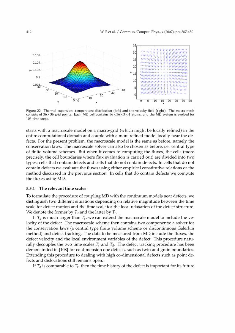
412 W. E et al. / Commun. Comput. Phys., 2 (2007), pp. 367-450
010
2030
40
010
2030
400.098
0.1
0.102
0.104
0.106
xy
T
0 5 10 15 20 25 30 35
0
5
10
15
20
25
30
35
x
y
Figure 22: Thermal expansion: temperature distribution (left) and the velocity field (right). The macro meshconsists of 36×36 grid points. Each MD cell contains 36×36×3×4 atoms, and the MD system is evolved for104 time steps.
starts with a macroscale model on a macro-grid (which might be locally refined) in theentire computational domain and couple with a more refined model locally near the de-fects. For the present problem, the macroscale model is the same as before, namely theconservation laws. The macroscale solver can also be chosen as before, i.e. central typeof finite volume schemes. But when it comes to computing the fluxes, the cells (moreprecisely, the cell boundaries where flux evaluation is carried out) are divided into twotypes: cells that contain defects and cells that do not contain defects. In cells that do notcontain defects we evaluate the fluxes using either empirical constitutive relations or themethod discussed in the previous section. In cells that do contain defects we computethe fluxes using MD.
5.3.1 The relevant time scales
To formulate the procedure of coupling MD with the continuum models near defects, wedistinguish two different situations depending on relative magnitude between the timescale for defect motion and the time scale for the local relaxation of the defect structure.We denote the former by Td and the latter by Tr.
If Td is much larger than Tr, we can extend the macroscale model to include the ve-locity of the defect. The macroscale scheme then contains two components: a solver forthe conservation laws (a central type finite volume scheme or discontinuous Galerkinmethod) and defect tracking. The data to be measured from MD include the fluxes, thedefect velocity and the local environment variables of the defect. This procedure natu-rally decouples the two time scales Tr and Td. The defect tracking procedure has beendemonstrated in [108] for co-dimension one defects, such as twin and grain boundaries.Extending this procedure to dealing with high co-dimensional defects such as point de-fects and dislocations still remains open.
If Td is comparable to Tr, then the time history of the defect is important for its future

W. E et al. / Commun. Comput. Phys., 2 (2007), pp. 367-450 413
x
t
x
t
Figure 23: Schematic of the adaptive modeling refinement. The left figure shows the case where Tr ≪Td. TheMD simulations are carried out inside the black boxes. The dashed lines represents the interface. The rightfigure shows the other case where Tr and Td are comparable. Here one has to keep track the local defectstructure for all time by MD simulation.
dynamics. There is no need to decouple the time scales since there is no time scale sepa-ration. In this case re-initializing the defect structure at macro time steps, as is commonlydone under the framework of HMM, is no longer needed and is in general less accurate.Instead, we should track the entire history of the local atomic structures near the defect.This situation often arises when dealing with small-size materials.
Fig. 23 illustrates the procedure for both cases.
5.3.2 MD boundary conditions
Another difference with the type B problems discussed earlier is that the local MD sim-ulations are no longer homogeneous. It then becomes highly non-trivial to impose theconstraints on the MD, which are typically done in the form of boundary conditions.There are two main issues that need to be addressed as far as boundary conditions areconcerned. The first is the handling of the phonons. Atomistic and continuum modelsrepresent phonons very differently. In atomistic models, phonons are represented in theform of lattice waves. In continuum models, they are represented by the temperaturefield. Ensuring consistency between these two vastly different representations is a highlynon-trivial problem. The second is the handling of defects. For example, dislocationsmight be emitted during crack propagation, and the MD boundary conditions have tohave the ability to allow such dislocations to leave the computational domain smoothly.
There has been relatively little work done on the second problem. The closest relatedwork is that of Shilkrot, Curtin and Miller on CADD (continuum-atomistic dislocationdynamics) [163, 164].
Much work has been done on the first problem, and a fairly complete picture hasemerged. We refer to [110, 184] for the details of this discussion.

414 W. E et al. / Commun. Comput. Phys., 2 (2007), pp. 367-450
a
0
01
η
22
00
a0
aa
0aa η η
Figure 24: Cubic and tetragonal phases for Ni-Al alloys.
5.3.3 Twin boundary dynamics in Ni-Al alloy
To see how these ideas can be applied to a realistic problem, we summarize the resultsof [108] for the example of twin boundary dynamics in a Ni62.5Al37.5 alloy. The atomisticmodel uses the EAM potential developed by Voter and Chen [176], which is specificallydesigned for Ni-Al alloys. At this percentage twin boundaries have been observed bothexperimentally [31] and in atomistic simulations (with this EAM potential) [17]. In par-ticular the EAM potential has predicted a tetragonal structure with three variants. Thecorresponding strain matrices can be written as,
U1 =
η1 0 00 η2 00 0 η2
, U2 =
η2 0 00 η1 00 0 η2
, U3 =
η2 0 00 η2 00 0 η1
. (5.7)
The cubic structure with lattice constant a0 =2.871 Ais chosen as the reference configura-tion. The parameters η1 and η2 can be thought of as being the stretch along the principalaxis illustrated in Fig. 24. The values of these parameters are obtained from MD simula-tion: η1 =1.2263 and η2 =0.9061.
For convenience the material is arranged so that the twin plane coincides with the y-zplane. The deformation corresponding to the undeformed variant I and variant II are:
A1 =
√2η1η2√η2
1+η22
0 0
η21−η2
2√2(η2
1+η22)
√η2
1+η22√
20
0 0 η2
, A2 =
√2η1η2√η2
1+η22
0 0
η22−η2
1√2(η2
1+η22)
√η2
1+η22√
20
0 0 η2
. (5.8)
The dynamics of the twin boundary is driven by a shear that is applied at the leftboundary. Away from the twin boundary, local MD simulations are performed to esti-mate the stress as was done for type B problems. Each such simulation involves 20×20×5atomic units and 2000 steps of time integration. Near the twin boundary the defect track-ing technique is applied to estimate the moving speed of the twin boundary and the localstrain and stress. Each such MD calculation is carried over a system with 120×20×8atomic units for 1200 time steps. In all the MD simulations the time step is taken to beδt=0.003 ps. Since the twin boundary simply moves in the x direction, and the continuum

W. E et al. / Commun. Comput. Phys., 2 (2007), pp. 367-450 415
−80 −60 −40 −20 0 20 40 60 80 100−60
−40
−20
0
20
40
60
80
100
120
x
y
Figure 25: Propagation of twin boundary under stress: shear stress is applied at the left boundary of the sample.The initial positions of the atoms are plotted in light color. The positions after 1.2 ps are plotted in dark color.
quantities do not have appreciable change in the y direction, the continuum equations canbe simplified to
∂t A11−∂xv1 =0,∂t A21−∂xv2 =0,∂tv1+∂xσ11 =0,∂tv2+∂xσ21 =0.
(5.9)
For simplicity the energy equation is neglected in this problem, and is replaced by con-straining the system at constant temperature. Other components of A are assumed not tochange in time.
Fig. 27 shows the numerical results at the macroscale level after some macro timesteps. As the twin boundary propagates, two elastic waves are generated and moveaway from the twin boundary.
To better understand the mechanism of twin boundary propagation, we plot in Fig. 25some results from the local MD simulation at the twin boundary. We first select an ar-bitrary plane of atoms and examine their positions at the initial and final times of theMD. Different variants of the twin are easily identified as rectangular lattices with differ-ent orientation. We see that at the end of the MD, the twin boundary has clearly movedforward (in a layer by layer fashion).
Next we examine what happens on the twin plane as it propagates forward. For thatpurpose we plot the atomic positions of the atoms on the twin plane. Fig. 26 clearlysuggests that the twin plane moves by a nucleation and propagation mechanism, verymuch similar to the mechanism of epitaxial growth of crystals. New variants are firstnucleated and form islands on the twin plane. The edges of the islands then propagateout and induce the transformation on the whole plane.
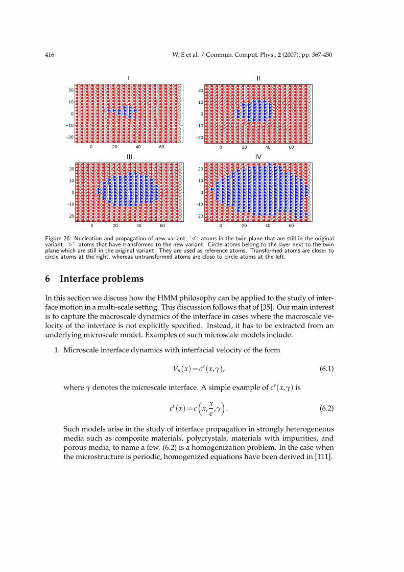
416 W. E et al. / Commun. Comput. Phys., 2 (2007), pp. 367-450
0 20 40 60
−20
−10
0
10
20
I
0 20 40 60
−20
−10
0
10
20
II
0 20 40 60
−20
−10
0
10
20
III
0 20 40 60
−20
−10
0
10
20
IV
Figure 26: Nucleation and propagation of new variant: ‘⊳’: atoms in the twin plane that are still in the originalvariant. ‘⊲’: atoms that have transformed to the new variant. Circle atoms belong to the layer next to the twinplane which are still in the original variant. They are used as reference atoms. Transformed atoms are closer tocircle atoms at the right, whereas untransformed atoms are close to circle atoms at the left.
6 Interface problems
In this section we discuss how the HMM philosophy can be applied to the study of inter-face motion in a multi-scale setting. This discussion follows that of [35]. Our main interestis to capture the macroscale dynamics of the interface in cases where the macroscale ve-locity of the interface is not explicitly specified. Instead, it has to be extracted from anunderlying microscale model. Examples of such microscale models include:
1. Microscale interface dynamics with interfacial velocity of the form
Vn(x)= cǫ(x,γ), (6.1)
where γ denotes the microscale interface. A simple example of cε(x,γ) is
cε(x)= c(
x,x
ǫ,γ)
. (6.2)
Such models arise in the study of interface propagation in strongly heterogeneousmedia such as composite materials, polycrystals, materials with impurities, andporous media, to name a few. (6.2) is a homogenization problem. In the case whenthe microstructure is periodic, homogenized equations have been derived in [111].

W. E et al. / Commun. Comput. Phys., 2 (2007), pp. 367-450 417
0 10 20 30 40−5
−4.5
−4
−3.5
−3
−2.5
−2
−1.5
−1
−0.5
0
v2
0 10 20 30 40−5
−4.5
−4
−3.5
−3
−2.5
−2
−1.5
−1
−0.5
0
v2
0 10 20 30 40−0.4
−0.3
−0.2
−0.1
0
0.1
0.2
0.3
0.4 A
21
0 10 20 30 40−0.4
−0.3
−0.2
−0.1
0
0.1
0.2
0.3
0.4 A
21
Figure 27: Left: the initial data for A2,1 and v2 (100 m/s); Right: the numerical results in 15 macro time steps.
2. Front propagation in phase-field models. Consider, for example, the Allen-Cahnequation
ut =ǫ∆u+1
ǫu(1−u2). (6.3)
It is well-known that for small ǫ, (6.3) describes the propagation of a front whoseinward normal velocity is the mean curvature of the front. In this case, we simplyhave to solve the mean curvature flow equation (instead of the microscale model(6.3)) in order to capture the large scale dynamics of the front. However, if the phasefield model takes a more complex form or if non-trivial chemical reactions occur atthe front, analytically deriving the effective dynamic laws for the front becomes adifficult task. Therefore it is of interest to develop numerical methods that capturethe large scale dynamics of the interface, and use only microscale models of thetype (6.3). Such ideas have been explored in the work of R. Klein et. al [155].
3. Discrete microscale models such as kinetic Monte Carlo algorithms or moleculardynamics. Examples include the dynamics of step edges on the surface of an epi-taxially grown crystal, grain boundaries in solids, and many more.

418 W. E et al. / Commun. Comput. Phys., 2 (2007), pp. 367-450
6.1 Macroscale solver: The level set method
As the macroscale solver we may use any of the conventional methods for interface dy-namics such as the level set method [127], front tracking [79], or the segment projectionmethod [173]. Here we will follow [35] and focus on the level set method. Alternativeapproaches can be found in [168].
In the framework of the level set method, an interface is described as the zero level setof a globally defined function, φ, called a level set function. All operations, in particular,the evolution, are then performed on this function in place of the interface of interest.The level set function φ satisfies the PDE:
φt+V ·∇φ=0,
where V is a globally defined velocity field. On the interface, this is equivalent to
φt±Vn|∇φ|=0, (6.4)
which involves the normal velocity only. In many problems, though, the velocity is onlynaturally specified at the interface. Many techniques are available to extend the velocityto the whole ambient space [7, 8, 87, 159].
6.2 Estimating the macroscale interface velocity
The data that need to be estimated from the microscale models are the normal velocitiesof the macroscale interface at each macroscale grid point. The first step is to locally recon-struct the interface. If the normal velocity of the macroscale interface is known to onlydepend on the orientation of the local tangent plane of the interface, then we may approx-imate the interface locally by a hyperplane. On the other hand, if the normal velocity isalso known to depend on the local curvature, a quadratic approximation is needed.
As an illustration, we first consider the homogenization problem. The level set repre-sentation of the microscale model in this case takes the form
φt+c(
x,x
ǫ
)|∇φ|=0, (6.5)
which describes motion in the normal direction at speed c. In this case, we can use thehyperplane reconstruction. [35] suggests working on a transformed coordinate througha change of variables so that this hyperplane coincides with the xn = 0-plane. Theoriginal microscale model (6.5) is then solved in a domain ∆ in the transformed space,rectangular with sides orthogonal to the coordinate axes, that should be larger than thesize of the periodic cell or the correlation length of c (see Fig. 28). Periodic boundaryconditions are imposed in the x1,x2,··· ,xn−1-directions and a periodic jump conditioncan be imposed in the xn-direction.
To extract the quantity of interest, at each microscale time step, the microscale Hamil-tonian is averaged in the central region ∆ of the domain to reduce spurious effects that

W. E et al. / Commun. Comput. Phys., 2 (2007), pp. 367-450 419
macroscale interface
vn
microscaleinterface
microscale computationaldomain ∆
γ
Figure 28: A pictorial description of the HMM setup showing the link between the macroscopic and microscopiclevels.
may arise from the boundary and the chosen boundary conditions. Denote this value byhǫ(t)
hε(t)=1
|∆|
∫
∆cε(x)|∇φ(x,t)|dx, (6.6)
the velocity of the front at the particular location is obtained from
Vn =1
|∇φ|∫ t∗
0hǫ(t)K
(t
t∗
)dt. (6.7)
Here K is an averaging kernel, as discussed earlier. Having obtained Vn at all the macroscalegrid points at the interface, the interface can be evolved using standard procedures in thelevel set method.
[35] also considered the case where the microscale model is described by a phase-fieldequation:
ut =∇·(
b(
x,x
ǫ
)u)+ǫ∇·
(a(
x,x
ǫ
)∇u)− 1
ǫ
∂V
∂u(u), (6.8)
where a(x,y)>0 and b(x,y) are smooth functions that are either periodic in y or stationaryrandom in y with rapidly decaying correlation at large distances and V is a double wellpotential with minima at u = α,β. For the details concerning this example, as well as thenumerical results, we refer to [35]. More recent results are found in the thesis [167].
7 Stochastic ODEs with multiple time scales
Consider the following generic example of ODEs with two time scales:
Xǫt = f (Xǫ
t ,Yǫt ,ǫ), Xǫ
0 = x,
Yǫt =
1
ǫg(Xǫ
t ,Yǫt ,ǫ), Yǫ
0 =y.(7.1)

420 W. E et al. / Commun. Comput. Phys., 2 (2007), pp. 367-450
Here (x,y)∈Rn×Rm, f (·)∈Rn and g(·)∈Rm are (possibly random) functions that areO(1) in ǫ, and ǫ is a small parameter representing the ratio of the time-scales in thesystem. We have assumed that the phase space can be decomposed into slow degrees offreedom x and fast ones y. Depending on the problem, we may be interested in the O(1)(advective) or O(ǫ−1) (diffusive) time-scales.
There has been numerous analytical work on systems of the type (7.1) [74,98,115,128].On the advective time-scale, if the dynamics for Yǫ
t with Xǫt = x fixed has an invariant
probability measure µǫx(dy) and the following limit exists:
f (x)= limǫ→0
∫
Rmf (x,y,ǫ)µǫ
x(dy), (7.2)
then in the limit as ǫ→0, Xǫt converges to the solution of
˙Xt = f (Xt), X0 = x. (7.3)
Leading order optimal prediction of Chorin et al. applied to this problem gives thesame result [41, 42]. On the diffusive time-scale, fluctuations become important. Withthe rescaled time s=ǫt, (7.1) becomes:
Xǫs =
1
ǫf (Xǫ
s ,Yǫs ,ǫ), Xǫ
0 = x,
Yǫs =
1
ǫ2g(Xǫ
s ,Yǫs ,ǫ), Yǫ
0 =y.
(7.4)
Under appropriate assumptions on f and g, the effective dynamics for Xǫs in the limit of
ǫ→0 is a stochastic differential equation,
˙Xs = b(Xs)+σ(Xs)Ws, X0 = x, (7.5)
where Ws is a Wiener process and the coefficients b and σ are expressed in terms of limitsof expectations similar to (7.2). Details can be found in [63]. We will only discuss thedynamics over the advective time scale, and refer to [63] for discussions on the diffusivetime scale.
In order to facilitate the discussion that we will present later on error analysis, weconsider a more special form of stochastic ODEs:
Xǫt = a(Xǫ
t ,Yǫt ,ε), Xǫ
0 = x,
Yǫt =
1
ǫb(Xǫ
t ,Yǫt ,ε)+
1√ǫ
σ(Xǫt ,Yǫ
t ,ε)Wt, Yǫ0 =y,
(7.6)
where a∈Rn, b∈Rm, σ∈Rm×Rd are deterministic functions and Wt is a d-dimensionalstandard Wiener process.
Based on the assumption that for small ε, the dynamics of Xεt is approximated by that
of˙Xt = a(Xt), X0 = x, (7.7)

W. E et al. / Commun. Comput. Phys., 2 (2007), pp. 367-450 421
an HMM type of strategy was independently proposed in [175]. The basic idea is to solve(7.7) with a macro-solver in which a is estimated by solving the micro-scale problem (7.6).
As the macroscale solver we may use any stable explicit ODE solver such as the for-ward Euler, Runge-Kutta, or a linear multi-step method. In the simplest case when for-ward Euler is selected as the macro-solver, we have
Xn+1 =Xn+ an∆t, (7.8)
where ∆t is the macro time step size.The data that need to be estimated is an which is an approximation of a(Xn). We
estimate this data in two steps:
1. We solve the second equation in (7.6) using a micro-solver for stochastic ODEs anddenote the solution by Yn,m where m labels the micro-time-steps. Multiple in-dependent replicas can be used, in which case we denote the solutions by Yn,m,jwhere j is the replica number.
2. We then define an approximation of a(Xn) by the following time and ensembleaverage:
an =1
MN
M
∑j=1
nT+N−1
∑m=nT
a(Xn ,Yn,m,j,ε),
where M is the number of replicas, N is the number of steps in the time averaging,and nT is the number of time steps we skip to eliminate transients.
For the micro-solver, for each realization we may use the following first order scheme
Yin,m+1 = Yi
n,m+1√
ε∑
j
σij(Xn,Yn,m,ε)ξjm+1
√δt
+1
εbi(Xn,Yn,m,ε)δt+
1
ε ∑jk
Aijk(Xn,Yn,m,ε)skjm+1δt, (7.9)
where δt is the micro-time-step size (note that it only appears in term of the ratio δt/ε=:∆τ), and
Aijk =∑l
(∂lσij)σlk. (7.10)
Here the derivatives are taken with respect to y. The random variables ξjm are i.i.d
Gaussian with mean zero and variance one, and
skjm =
12 ξk
mξjm+z
kjm, k< j,
12 ξk
mξjm−z
jkm, k> j,
12
((ξ
jm)2−1
), k= j,

422 W. E et al. / Commun. Comput. Phys., 2 (2007), pp. 367-450
0 1 2 3 4 5 6−1.5
−1
−0.5
0
0.5
1
1.5
t
Figure 29: The comparison between Xn and Xn produced by the multiscale scheme with p=4 (black curves).Also shown is the fast process Yn,nT+N used in the micro-solver (grey curve).
where zkjm are i.i.d with Pz
kjm = 1/2= Pz
kjm =−1/2= 1/2. High order schemes are
discussed in [63]. For the initial condition, we take Y0,0 =0 and
Yn,0 =Yn−1,nT+N−1, (7.11)
i.e. the initial values for the micro variables at macro-time-step n are chosen to be theirfinal values from macro-time-step n−1. This choice of initial condition is not necessaryfor the convergence of the scheme, e.g.
Yn,0 =0 (7.12)
would work as well, but it improves the convergence properties, as we will discuss inSection 9.2.3.
As an illustration, consider the following example with (x,y)∈R2:
Xt =−Yt−Y3t +cos(πt)+sin(
√2πt), X0 = x,
Yt =−1
ǫ(Yt+Y3
t −Xt)+1√ǫ
Wt, Y0 =y.(7.13)
From (7.7) the effective equation for Xt is
˙Xt =−Xt+cos(πt)+sin(√
2πt), X0 = x. (7.14)
We choose the following numerical parameters:
(T0,∆t,δt/ε,nT ,M,N)=(6, 0.01, 0.01×2−p, 100, 1, 10×23p). (7.15)
The results for p=2 is shown in Fig. 29, and compared with the solution of the effectiveequation for Xt.
W. E et al. / Commun. Comput. Phys., 2 (2007), pp. 367-450 423
8 Exploring statistical self-similarity: An example without scale
separation
8.1 General strategy for data estimation
In the problems discussed above, scale separation was very important for the efficiencyof HMM: It allows us to choose small microscale simulation domain and still retain suf-ficient accuracy for the estimated data. It is important to realize that this is not the onlysituation for which HMM works efficiently. The underlying philosophy is more generaland it works as follows. Suppose that the size of the macroscale mesh is H. We need toestimate some effective data such as transport coefficients at that scale, which is a func-tion of H. Let us denote by f = f (L) the value of that data at the scale L. If there is scaleseparation in the system, then f (L) is essentially independent of L:
f (L)≈Const (8.1)
as long as L is much larger than some characteristic scale of the microscopic model, whichmight just be the correlation length. This allows us to take advantage of the scale sep-aration by choosing the size of the microscale simulation domain, δ, to be much largerthan the microscopic scale, but still much smaller than H. However, so long as the scaledependence of f = f (L) is of a simple form with only few parameters, we can make useof this simple relationship by performing a few (not just one as was done for problemswith scale separation) small scale simulations and use the results to predict the neededquantities at a much larger scale. One example of such a situation is when the systemexhibits local self-similarity. In this case the dependence in (8.1) is of the form
f (L)=C0Lβ
with only two parameters. Therefore we can use results of microscopic simulations attwo different scales to predict the result at a much larger scale, namely H.
This is a poor-man’s version of the renormalization group method. Other examplesof numerical methods that use renormalization ideas are found in [37, 38].
8.2 Transport on a percolation network at criticality
This idea was demonstrated in [66] on the example of effective transport on a two-dimensional bond percolation network at the percolation threshold.
In the standard two dimensional bond percolation model with parameter p, 0≤ p≤1,we start with a square lattice, each bond of the lattice is either kept with probabilityp or deleted with probability 1−p. Of particular interest is the size of the percolationclusters formed by the remaining bonds in the network (see Fig. 30 for a sample of bondpercolation). The critical value for this model is at p = p∗ = 0.5. For an infinite lattice, ifp < p∗, the probability of having infinite size clusters is zero. For p > p∗, the probability

424 W. E et al. / Commun. Comput. Phys., 2 (2007), pp. 367-450
Figure 30: Bond percolation network on a square lattice at p=0.5.
of having infinite size clusters is 1. Given the parameter value p, the network has acharacteristic length scale – the correlation length, denoted by ξp. As p→ p∗ , ξp divergesas
ξp∼|p−p∗ |α, (8.2)
where α =−4/3 (see [152]). At p = p∗, ξp = ∞. In this case, the system has a continuumdistribution of scales, i.e. it has clusters of all sizes. In the following we will consider thecase when p= p∗.
We are interested in macroscopic transport on such a network. To study transport,say of some pollutants whose concentration density will be denoted by c, we embedthis percolation model into a domain Ω in R2. We denote by ε the bond length of thepercolation model, and L the length scale for the domain Ω. We will consider the casewhen ε/L is very small.
The basic microscopic model is that of mass conservation. Denote by Si,j,i, j=1,··· ,Nthe (i, j)-th site of the percolation network, and ci,j the concentration at that site. Definethe fluxes
the flux from right f ri,j = Bx
i,j(ci+1,j−ci,j),
the flux from left f li,j = Bx
i−1,j(ci−1,j−ci,j),
the flux from top f ti,j = B
yi,j(ci,j+1−ci,j),
the flux from bottom f bi,j = B
yi,j−1(ci,j−1−ci,j).
Here the various B’s are the bond conductivities for the specified bonds. The bond con-ductivity is zero if the corresponding bond is deleted, and 1 if the bond is retained. Ateach site Si,j, from mass conservation, we have
f ti,j+ f b
i,j+ f ri,j+ f l
i,j =0, (8.3)
W. E et al. / Commun. Comput. Phys., 2 (2007), pp. 367-450 425
i.e. the total flux to this site is zero. This will be our microscale model.For the macroscale solver, we choose a finite volume scheme over a macroscale grid
ΩH where H is the size of the finite volume cell (see Fig. 3). The data that need to beestimated from the microscale model, here the percolation model, are the fluxes at themid-points of cell boundaries. Since the present problem is linear, we only need to es-timate the effective conductivity for a network of size H. We note that at p = p∗, theeffective conductivity is strongly size-dependent. In fact there are strong evidences thatthe following relation holds [89]:
κL =C0Lβ, (8.4)
where κL is the mean effective conductivity at size L. This is confirmed in Fig. 31 wherewe show a log-log plot of the effective conductivity as a function of scale.
Our basic strategy is to make use of such a relation to estimate the effective fluxes inthe case when ε≪H. For this purpose, we perform a series of local microscopic simula-tions on systems of size L1 and L2 where ε≪ L1 < L2 ≪H. From the results we estimateκL1
and κL2. We then use these results to estimate the parameter values C0,β in (8.4). Once
we have these parameters, we can use (8.4) to predict κH.One interesting question is the effect of statistical fluctuations. To see this we plot
in Fig. 32 the actual and predicted (using self-similarity) values of the conductivity on asub-lattice of size L = 128 for a number of realizations of the percolation network. Thepredicted values are computed using simulated values from sub-lattices with L=16 andL = 32. The predicted values have obviously larger fluctuations than the actual values,implying that the fluctuations are amplified in the process of predicting the mean values.Nevertheless the mean values are predicted with reasonable accuracy, considering therelatively small size of the network.
More numerical results, including some results of the multiscale method, can befound in [66].
9 Error analysis
Error analysis for multiscale methods presents a new challenge to numerical analysis,particularly for problems involving multi-physics. Since multiscale methods are rela-tively new, and their errors typically involve several different contributions, rigorousresults on error control are very much desired in order to help understanding basic is-sues such as stability and accuracy of multiscale methods. Indeed, to be able to developa general strategy for error analysis was one of the main motivations for developing theHMM framework.
To begin with, what should we take as the exact or reference solution, to be comparedwith the numerical solution of a multiscale method? In general, we should not take thedetailed solution of the microscopic problem as the reference solution, since approximat-ing that would usually require solving the full microscopic problem, and therefore defeat
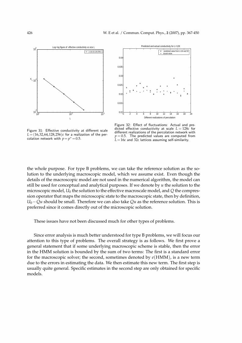
426 W. E et al. / Commun. Comput. Phys., 2 (2007), pp. 367-450
101 10 2 10 310−2
10−1
100 Log−log figure of effective conductivity vs size L
L
KL
L=(16,32,128,256) ε
Figure 31: Effective conductivity at different scaleL=(16,32,64,128,256)ε for a realization of the per-colation network with p= p∗ =0.5.
0 2 4 6 8 10 12 14 16 18 200.01
0.015
0.02
0.025
0.03
0.035
0.04
Predicted and actual conductivity for L=128
Different realizations of percolation
predicted value from L=16 and 32acutal value
Figure 32: Effect of fluctuations: Actual and pre-dicted effective conductivity at scale L = 128ε fordifferent realizations of the percolation network withp = 0.5. The predicted values are computed fromL=16ε and 32ε lattices assuming self-similarity.
the whole purpose. For type B problems, we can take the reference solution as the so-lution to the underlying macroscopic model, which we assume exist. Even though thedetails of the macroscopic model are not used in the numerical algorithm, the model canstill be used for conceptual and analytical purposes. If we denote by u the solution to themicroscopic model, U0 the solution to the effective macroscale model, and Q the compres-sion operator that maps the microscopic state to the macroscopic state, then by definition,U0−Qu should be small. Therefore we can also take Qu as the reference solution. This ispreferred since it comes directly out of the microscopic solution.
These issues have not been discussed much for other types of problems.
Since error analysis is much better understood for type B problems, we will focus ourattention to this type of problems. The overall strategy is as follows. We first prove ageneral statement that if some underlying macroscopic scheme is stable, then the errorin the HMM solution is bounded by the sum of two terms: The first is a standard errorfor the macroscopic solver; the second, sometimes denoted by e(HMM), is a new termdue to the errors in estimating the data. We then estimate this new term. The first step isusually quite general. Specific estimates in the second step are only obtained for specificmodels.

W. E et al. / Commun. Comput. Phys., 2 (2007), pp. 367-450 427
9.1 Error analysis of the HMM-FEM
Our first example is the HMM finite element method discussed earlier. We will alwaysassume that aε(x) is smooth, symmetric and uniformly elliptic:
λI≤ aε ≤ΛI (9.1)
for some λ,Λ>0 which are independent of ε. We will assume that the quadrature formulaused in (3.3) is exact for polynomials of degree 2k−2 for k>1 and k for k=1.
We will use standard notions for Sobolev spaces: ‖·‖1 and ‖·‖0 denote H1 and L2
norms respectively, and ‖·‖1,∞ denotes the W1,∞ norm.As the first step, we will compare the HMM solution to the solutions of a macroscale
model of the form:−div
(A(x)∇U0(x)
)= f (x), x∈D,
U0(x)=0, x∈∂D.(9.2)
The following results are proved in [65].
Theorem 9.1. Denote by U0 and UHMM the solution of (9.2) and the HMM solution, respec-tively. Let
e(HMM)= maxxℓ∈KK∈TH
‖A(xℓ)−AH(xℓ)‖,
where ‖·‖ is the Euclidean norm. If U0 is sufficiently smooth, then there exists a constant Cindependent of ε,δ and H, such that
‖U0−UHMM‖1≤C(
Hk+e(HMM)), (9.3)
‖U0−UHMM‖0≤C(
Hk+1+e(HMM)). (9.4)
In addition, there exit constants C0 and H0 such that if e(HMM)|lnH|<C0, then for all H≤H0,
‖U0−UHMM‖1,∞ ≤C(
Hk+e(HMM))|lnH|. (9.5)
So far no assumption on the form of aε(x) or A(x) is necessary. U0 can be the solutionof an arbitrary macroscopic equation with the same right-hand side as in (2.17). Of coursefor UHMM to converge to U0, i.e., e(HMM)→0, U0 must be chosen as the solution of thehomogenized equation, which we now assume exists. To obtain quantitative estimateson e(HMM), we must restrict ourselves to more specific situations.
The simplest example of such a specific problem is when
aε(x)= a(
x,x
ε
), (9.6)
where a(x,y) is either periodic in y, in which case we assume the period to be I =[−1/2,1/2]d , or random but stationary under shifts in y, for each fixed x ∈ D. In bothcases, it has been shown that [18, 129]
‖uε(x)−U0(x)‖0 →0, (9.7)
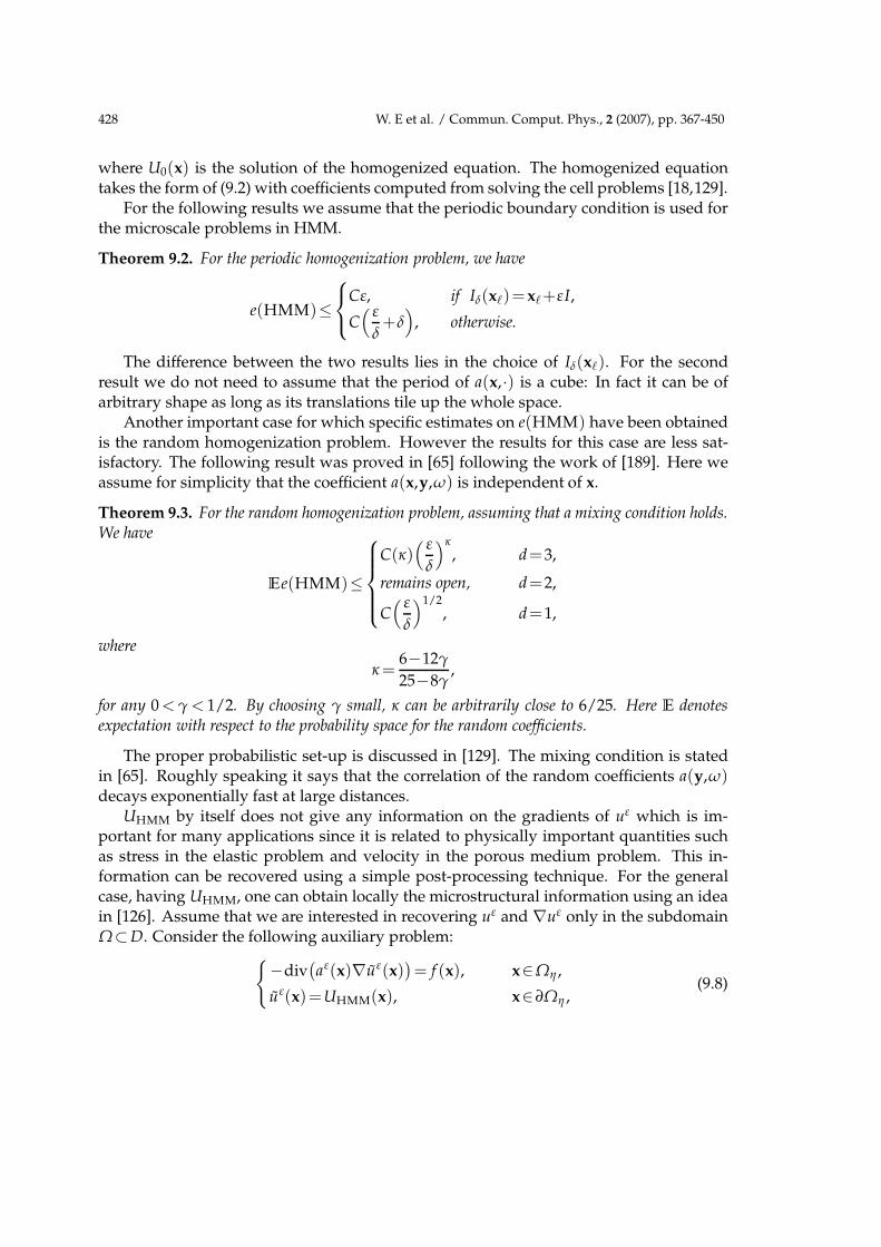
428 W. E et al. / Commun. Comput. Phys., 2 (2007), pp. 367-450
where U0(x) is the solution of the homogenized equation. The homogenized equationtakes the form of (9.2) with coefficients computed from solving the cell problems [18,129].
For the following results we assume that the periodic boundary condition is used forthe microscale problems in HMM.
Theorem 9.2. For the periodic homogenization problem, we have
e(HMM)≤
Cε, if Iδ(xℓ)=xℓ+εI,
C( ε
δ+δ)
, otherwise.
The difference between the two results lies in the choice of Iδ(xℓ). For the secondresult we do not need to assume that the period of a(x,·) is a cube: In fact it can be ofarbitrary shape as long as its translations tile up the whole space.
Another important case for which specific estimates on e(HMM) have been obtainedis the random homogenization problem. However the results for this case are less sat-isfactory. The following result was proved in [65] following the work of [189]. Here weassume for simplicity that the coefficient a(x,y,ω) is independent of x.
Theorem 9.3. For the random homogenization problem, assuming that a mixing condition holds.We have
Ee(HMM)≤
C(κ)( ε
δ
)κ, d=3,
remains open, d=2,
C( ε
δ
)1/2, d=1,
where
κ =6−12γ
25−8γ,
for any 0 < γ < 1/2. By choosing γ small, κ can be arbitrarily close to 6/25. Here E denotesexpectation with respect to the probability space for the random coefficients.
The proper probabilistic set-up is discussed in [129]. The mixing condition is statedin [65]. Roughly speaking it says that the correlation of the random coefficients a(y,ω)decays exponentially fast at large distances.
UHMM by itself does not give any information on the gradients of uε which is im-portant for many applications since it is related to physically important quantities suchas stress in the elastic problem and velocity in the porous medium problem. This in-formation can be recovered using a simple post-processing technique. For the generalcase, having UHMM, one can obtain locally the microstructural information using an ideain [126]. Assume that we are interested in recovering uε and ∇uε only in the subdomainΩ⊂D. Consider the following auxiliary problem:
−div
(aε(x)∇uε(x)
)= f (x), x∈Ωη ,
uε(x)=UHMM(x), x∈∂Ωη ,(9.8)

W. E et al. / Commun. Comput. Phys., 2 (2007), pp. 367-450 429
where Ωη satisfies Ω ⊂ Ωη ⊂ D and dist(∂Ω,∂Ωη) = η. We then have: There exists aconstant C such that
(∫−
Ω|∇(uε−uε)|2x
)1/2≤ C
η‖uε−UHMM‖L∞(Ωη). (9.9)
There is a much simpler procedure for the periodic homogenization problem [55].Consider the case when k=1 and choose Iδ =xK+εI, where xK is the barycenter of K. Wealso assume that the quadrature point in the element K is at xK. Define uε by:
1. uε|Iδ= vε
K, where vεK is the solution of (3.4) with the boundary condition that vε
K−UHMM is periodic with period εI and
∫Iδ(uε−UHMM)(x)dx=0.
2.(uε−UHMM
)|K is periodic with period εI.
We then have [65]
Theorem 9.4. Let uε be defined as above. Then
(∑
K∈TH
‖∇(uε−uε)‖20,K
)1/2≤C
(√ε+H
). (9.10)
Similar results are also proved for nonlinear elliptic problems. For details, see [65].
[188] presents systematic numerical studies on the effect of the boundary conditionsfor the microscale problems as well as the microscale cell size.
9.2 Dynamic problems
The main strategy proposed in [56] is to compare the HMM solution with that of an un-derlying macroscale solver, or an effective macroscale method. The basic result, provedin [56], is that if this effective macroscale method is stable and k-th order accurate, then
||UHMM−U0||≤ ||UHMM−UH||+||UH−U0||≤C(e(HMM)+(∆t)k), (9.11)
where U0 is the solution of the macroscale model, e(HMM) is the error in the esti-mated effective force. In proving (9.11), it is assumed that both HMM and the effectivemacroscale method are expressed in the form:
Un+1 =Un+∆tFε(U), (9.12)
Un+1 = Un+∆tF(U), (9.13)
and e(HMM) is defined as
e(HMM)=maxU
‖F(U)−Fε(U)‖. (9.14)

430 W. E et al. / Commun. Comput. Phys., 2 (2007), pp. 367-450
We also have:
||Quε−UHMM||≤ ||Quε−U0||+||UH−U0||+||UHMM−UH||. (9.15)
Here the first term on the right-hand side is due to the error in the effective model; thesecond term is due to the error in the macroscale solver; the third term is the HMMerror. Denote by ε the parameter that characterizes the small scale in the problem. (9.15)suggests an estimate of the type:
||Quε−U0||≤C(εα+(∆t)k +e(HMM)). (9.16)
We now apply this general result to some concrete examples.
9.2.1 ODEs with multiple time scales
The problems and algorithms were discussed in Section 2.2.1. If we apply the generalprinciples discussed above, we get:
Theorem 9.5. HMM is stable if the macroscale solver is stable. Moreover for any given constantT there exists a constant C such that
|En|≤C((∆t)k +e(HMM))
if n∆t≤T, where En is the error between the HMM solution and the slow component of the exactsolution (a precise definition is given below), k is the order of the macroscale solver, e(HMM) isthe error in the estimation of the macroscale data.
Next we estimate e(HMM). This depends on a number of important factors in HMM,in particular the filter K. We first discuss the case of dissipative systems and considerfor simplicity the example in (2.4). We will further assume that f and g are smooth andbounded, and that Zn,0 is bounded.
In the limit as ε→ 0, one expects that x will be close to f (y), and hence the effectivedynamics for the slow variable y is given by
˙y= g( f (y),y)=G(y). (9.17)
In fact, we can easily prove the following: If we denote by (xε,yε) the solution of (2.4) andif yε(0)= y(0), then
|yε(t)−y0(t)|≤C1exp
(− t
ε
)+C2ε.
Let us first consider the case when the macroscale solver is forward Euler. In this case wecan express HMM as:
yn+1 =yn +∆tg(yn).

W. E et al. / Commun. Comput. Phys., 2 (2007), pp. 367-450 431
Let En =yn−y0(tn), where tn =n∆t, for n∆t≤T. We have
En+1−En
∆t= g(yn)−G(y0(tn))+O(∆t)
=G(yn)−G(y0(tn))+ g(yn)−G(yn)+O(∆t)
=G′(y0(tn)+θEn)En+ g(yn)−G(yn)+O(∆t).
If we let L=max|G′(y)|, then we get
|En|≤ eLt(C∆t+ maxn∆t≤T
|g(yn)−G(yn)|),
where C=maxt≤T |y′′0 (t)|. Here the first term on the right-hand side is the standard trun-cation error at the macroscale. The second term |g(yn)−G(yn)| is what we usually calle(HMM). With (2.10), it is a simple matter to prove [53]:
e(HMM)≤C(
∆t+|1−δt/ε|N)
. (9.18)
In the general case when k-th order stable macroscale solvers are used, we have [53]:
Theorem 9.6. Assume that the macroscale solver is k-th order accurate and stable, i.e. for linearmulti-step methods the root condition is satisfied. Let A(λδt) be the amplification factor of themicroscale solver for the ODE y =−λy. Then there exists a constant C, independent of ∆t,ε,δtand N, such that, for n∆t≤T,
|En|≤C(
∆tk +|A(δt/ε)|N)
.
Next we consider the oscillatory case. As before we will discuss a simple and yetcanonical example, namely (2.5). The dynamics for the slow variable I obeys the equation
˙I =1
2π
∫ 2π
0g(ϕ, I)dϕ=G( I). (9.19)
See for example [11]. We will assume that ω(I) never vanishes:
ω(I)≥ω0 >0. (9.20)
We will restrict ourselves to the situation when the weights Km,N are of the form
Km,N =K0
(1− m
N
)(9.21)
for m=0,1,.. .,N, where K0 is a filtering kernel.A crucial component in the analysis in this case is the effect of the kernel K0. This is
examined in detail in [69]. Consider an example for which the microscopic data takes theform:
f ε(t)= f0(t)+ f1
(t
ε
),

432 W. E et al. / Commun. Comput. Phys., 2 (2007), pp. 367-450
where f1(τ) is periodic in τ with period 1. The macroscale component of f ε(t) is
F(t)= f0(t)+∫ 1
0f1(τ)dτ.
The macroscale data of interest is F0 = F(0). Assume that the F-estimator has the form
F0 =1
T
∫ T
0K0
(1− τ
T
)f ε(τ)dτ.
Then we have:
Lemma 9.1. Assume that K0 satisfies the following conditions
1. (A1). Moment condition
∫ 1
0K0(τ)dτ =1,
∫ 1
0(1−τ)αK0(τ)dτ =0
for α=1,2,.. .ℓ−1.
2. (A2). Regularity condition
K(α)0 (0)=K
(α)0 (1)=0
for α=0,1,.. . ,q−1 and∫ 1
0|K(α)
0 (τ)|ατ <+∞
for α=0,1,.. . ,q.
Then
|F0− F0|≤C(
Tℓ+( ε
T
)q).
Using this result, we obtain:
Theorem 9.7. Under the same assumption as before, we have
|En|≤C
((∆t)k +
(δt
ε
)r
+( ε
Nδt
)q)
,
where r=min(l,p) and p is the order of the microscale solver.
As expected, the size of δt should be chosen to resolve the small time scale ε, and Nshould be large enough so that Nδt is larger than ε in order to sample adequately thedynamics at the small scale.
W. E et al. / Commun. Comput. Phys., 2 (2007), pp. 367-450 433
9.2.2 The effect of the fast variable reinitialization
The error estimates given in the last subsection were for the general case when the ini-tialization of the fast variables in the microscale solver is quite arbitrary. Suitable reini-tialization of the fast variables at each macro-time-step may result in significant gain inefficiency. Precise estimates are given below for the case of stochastic ODEs, but it isuseful to first illustrate the influence of fast variables initialization on a simple example(2.4).
Suppose that the initial condition for (2.9) is taken to be xn,0=0. Then N must be takenlarge enough so that (2.9) has converged to sufficient accuracy, i.e. xn,N ≈ f (yn), and theerror estimate for e(HMM) is given in (9.18).
Suppose on the contrary that we take xn,0 = xn−1,N. Then it can be shown that theerror estimate improves to
e(HMM)≤C
(∆t+
ε∆t
Nδt+∆t
∣∣∣∣1−δt
ε
∣∣∣∣N)
, (9.22)
which indicates, in particular, that the scheme converges as ∆t,δt → 0 provided thatε∆t/Nδt → 0. Notice that this can happen even if N = 1. Notice also that accuracy re-quires that
ε∆t/Nδt≪1,
whereas gaining in efficiency in the sense of (1.1) requires
∆t/Nδt≫1.
For small ε both constraints can be satisfied at the same time.The simplest way to justify (9.22) is to re-write (2.9) as
xn,m+1 = xn,m− 1
γ
∆t
N(xn,m− f (yn)), (9.23)
where
γ=ε∆t
Nδt. (9.24)
It is easy to see that in the limit as δt, ∆t→0 with γ kept fixed, HMM is consistent withthe modified equation
x=− 1
γ(x− f (y)),
y= g(x,y).(9.25)
If γ≫ε, this equation is less stiff than (2.4) and correspondingly HMM gains in efficiencyover a direct scheme for (2.4). On the other hand, for ε≪ 1 it is possible to also satisfy1≫γ≫ ε. In this case, the y component of the solutions of (2.4) and (9.25) remains closebecause of the existence of a limiting dynamics. But the choice of γ is now dictated bythe error tolerance and not by the value of ε in the original equation.
434 W. E et al. / Commun. Comput. Phys., 2 (2007), pp. 367-450
9.2.3 Stochastic ODEs with multiple time scales
Here we discuss some of the results proved in [63] for stochastic ODEs. The algorithmswere described in Section 7. Again we will focus on the case of advective time scale.Diffusion time scale was considered in [63].
We will make the following assumptions:
1. The coefficients a, b and σ, viewed as functions of (x,y,ε), are in C∞b , a and σ are
bounded. Here C∞b is the space of smooth functions with bounded derivatives of
any order.
2. There exists an α>0 such that ∀ (x,y,ε),
|σT(x,y,ε)y|2 ≥α|y|2.
3. There exists a β>0 such that ∀ (x,y1,y2,ε),
〈(y1−y2),(b(x,y1,ε)−b(x,y2,ε))〉+‖σ(x,y1,ε)−σ(x,y2,ε)‖2 ≤−β|y1−y2|2,
where ‖·‖ denotes the Frobenius norm.
Under these assumptions, we have:
Theorem 9.8. Assume that the macro solver is stable and k-th order accurate for (7.7). Then forany T0 >0, there exists a constant C>0, independent of (ǫ, ∆t, δt, nT, M, N), such that
supn≤T0/∆t
E|Xǫtn−Xn|≤C
(√
ǫ+(∆t)k +eD
), (9.26)
where tn =n∆t, and
eD =(δt/ε)ℓ+e−
12 βnT(δt/ε)
√N(δt/ε)+1
(R+√
R)+
√∆t√
M(N(δt/ε)+1). (9.27)
Here ℓ is the weak order of the micro solver,
R=∆t
1−e−12 β(nT+N−1)(δt/ε)
, (9.28)
if the fast variable is initialized as in (7.11) and R=1 if the fast variable is initialized as in (7.12).
The basic idea for proving this result is as follows. The error |Xǫtn−Xn| in (9.26) is
decomposed into three parts:
1. |Xǫt −Xt|, where Xt is the solution of the effective equation (7.7).
2. |Xtn−Xn|, where Xn is the approximation of Xtn given by the selected macro solverassuming that a(x) is known.
3. |Xn−Xn|.

W. E et al. / Commun. Comput. Phys., 2 (2007), pp. 367-450 435
The first part is the error in the averaging principle itself. As shown in [63], we have
sup0≤t≤T0
E|Xǫt −Xt|≤C
√ǫ.
This is the first term in (9.26). The second part is a standard ODE estimate:
supn≤T0/∆t
|Xtn −Xn|≤C(∆t)k. (9.29)
This is the second term in (9.26). The third part, eD, accounts for the error caused byusing an instead of a(Xn) in the macro solver. Here the term (δt/ε)ℓ is due to the micro-time discretization which induces a difference between the invariant measures of thecontinuous and discrete dynamical systems. The term
e−12 βnT(δt/ε)
√N(δt/ε)+1
(R+√
R)
accounts for the errors caused by relaxation of the fast variables. The factor R reflectsthe influence of the particular initialization procedure used for the fast variables at eachmacro time step. Different initialization leads to similar estimates but with different val-ues of R. For example if we use Yn,0 =0, then R=1. Finally, the term
√∆t√
M(N(δt/ε)+1)
accounts for the sampling errors after the fast variable reaches local equilibrium. This isa central limit theorem type of estimate.
The estimate (9.26) suggests a somewhat surprising fact, namely that the HMM schemeconverges as ∆t→ 0, δt→ 0 on any sequence such that R→ 0, even if we take only onerealization and one micro time step per macro time step, M=1, nT =1, N =1. In this caseR=∆t/(δt/ε) to leading order. This is the consequence of the particular re-initializationprocedure that we have adopted (see (7.11)), and it is a manifestation of the point madein the last subsection.
We now discuss how these results play out in actual computations. We will adopt themore accurate initialization procedure for the fast variable. When
Nm(δt/ε)=(nT +N−1)(δt/ε)>1,
we have R=∆t plus higher order terms, and
supn≤T0/∆t
E|Xn−Xn|≤C
((δt/ε)ℓ+
e−12 βnT(δt/ε)
√∆t√
N(δt/ε)+1+
√∆t√
M(N(δt/ε)+1)
). (9.30)

436 W. E et al. / Commun. Comput. Phys., 2 (2007), pp. 367-450
0 1 2 3 4 5 6 7
10−3
10−2
10−1
p
Err
or
Figure 33: The error Eℓp = (∆t/T0)∑n≤⌊T0/∆t⌋ |Xn−Xn| as a function of p when ℓ = 1 (circles) and ℓ = 2
(squares). Also shown is the predicted estimated, 0.1×2−p (dashed line).
Table 3: The computed values for the error Eℓp.
p=0 p=1 p=2 p=3 p=4 p=5 p=6 p=7
ℓ=1 .058 .070 .032 .019 .0096 .0067 .0025 .00076
ℓ=2 .045 .059 .022 .021 .0098 .0064 .0033 .0014
Here ∆t is taken as a fixed parameter. Suppose that we want to bound the error by O(2−p)for p=0,1,.. . and assume that M=1. Then as in [63], we find that the optimal parametersare
δt/ε=O(2−p/ℓ), nT =O(1), N =O(2p(2+1/ℓ)),
which gives
cost =nT +N−1
∆t=O(2p(2+1/ℓ))
independent of ε. The magnitudes of the errors for various p and ℓ=1,2 are listed in thefollowing table and shown in Fig. 33. As predicted, we the error scales as Eℓp =O(2−ℓp).
9.2.4 Other examples
We briefly mention a few other examples that have been analyzed. The parabolic homog-enization problem has been analyzed in [3, 55, 120]. The structure of the analysis is verysimilar to the examples discussed here. In particular, [120] gives results that are similarto the ones discussed here for the elliptic homogenization problem. Error analysis andcareful numerical studies for the hyperbolic homogenization problem were presentedin [33, 34].
Examples with discrete microscale models were considered in [61]. The discrete mod-els can be molecular dynamics or kinetic Monte Carlo methods. The macroscale model
W. E et al. / Commun. Comput. Phys., 2 (2007), pp. 367-450 437
considered in [61] was gas dynamics or general nonlinear conservation laws. It is provenin [61] that the e(HMM) error consists of three parts: the relaxation error, the error dueto the finite size of the simulation domain for the micro model, and the sampling error.Clearly as the system size increases, the finite size effect decreases but the relaxation errorincreases. Therefore this result gives some suggestions on how to choose the size of themicroscale simulation domain. Unfortunately there are very few explicit results on thedependence of these errors on the domain size. All known results are proved for latticemodels. We refer to [61] for a discussion on this issue.
10 Limitations of HMM
As was discussed in [56], there are problems for which HMM does not work well. Oneclass of such problems are problems for which the time history of the detailed microstruc-tural behavior has to be parametrized in order to determine the macroscale properties.One such example is the homogenization problem for the Carleman model, discussedin [56]. Consider the Carlman equation with multiscale initial data:
∂u
∂t+
∂u
∂x=v2−u2,
∂v
∂t− ∂v
∂x=u2−v2,
u(x,0)= a(x,x/ε),
v(x,0)=b(x,x/ε),
(10.1)
where a(x,y),b(x,y) are assumed to be smooth and 1-periodic in y. The homogenizedequation for this problem is given by [170]:
∂u
∂t+
∂u
∂x=∫ 1
0v(x,y,t)2dy−u2,
∂v
∂t− ∂v
∂x=∫ 1
0u(x,y,t)2dy− v2,
u(x,y,0)= a(x,y),
v(x,y,0)=b(x,y).
(10.2)
Tartar proved [170]:
limε→0
(∣∣∣∣u(x,t)−u
(x,
x−t
ε,t
)∣∣∣∣+∣∣∣∣v(x,t)− v
(x,
x+t
ε,t
)∣∣∣∣)
=0.

438 W. E et al. / Commun. Comput. Phys., 2 (2007), pp. 367-450
Here the natural macroscale variables U are the weak limits of the full microscale solu-tions:
U(x,t)=∫ 1
0u(x,y,t)dy= lim
δ→0
(limε→0
∫Kδ(x−z)u(z,t)dz
),
V(x,t)=∫ 1
0v(x,y,t)dy= lim
δ→0
(limε→0
∫Kδ(x−z)v(z,t)dz
),
where Kδ is some kernel compactly supported in (−δ,δ) with,
∫ δ
−δKδ(x)dx=1.
However for this problem, there is no time scale separation between the dynamics of(U,V) and the remaining components of (u,v), such as higher order moments. In fact, toobtain information on (U,V), one has to keep track of the dynamics of the microstructure.Therefore a blind application of HMM will give wrong results.
As was shown in [67], this particular problem can be effectively treated using a com-bination of the particle method and a proper sampling procedure for the microstructure.
A second example with a very similar feature is the transport equation with oscilla-tory velocity fields
∂tu+∂x1
(a( x2
ε
)u)
=0. (10.3)
The homogenized equation for this problem is [170]
∂tU+ a∂x1U =∂2
x1
∫ α
−αdω(γ)
∫ t
0dsU(x1+γ(t−s),x2,s) (10.4)
and it shows memory dependence. Here ω is some kernel that depends on a, a is theaverage of a over its period. We refer to [55] for discussions of this example.
Both examples can be treated by the fiber bundle idea discussed earlier. For the ex-ample of Carleman equation, we can view the y-space as being the fiber. Same can besaid about the linear transport equation. One can then design numerical methods basedon the idea of evolving the microstructure over the fiber. An application of this idea ispresented in [187] for the transport equation.
Another limitation of HMM concerns with the a priori assumption on the constitutiverelation, which is reflected in the constraints on the microscale solver. A crucial advan-tage of HMM is that it does not need the full knowledge of the macroscale model. Butsome knowledge about the macroscale model is important, as we now illustrate.
Consider the problem
∂tu+∇·(
b( x
ε
)u)
=∇·(
a( x
ε
)∇u)
, (10.5)
where b and a are smooth periodic functions with period 1. The homogenized equationfor (10.5) is given by
∂tU+∇·(bU)=∇·(A∇U), (10.6)

W. E et al. / Commun. Comput. Phys., 2 (2007), pp. 367-450 439
where A is the homogenized coefficient for the case when b = 0, b is the average of bover its period. Without knowing that the effective macroscale flux should depend onthe derivative of the macroscale variable U, we might use HMM as in Section 2.2.2, andimpose as constraints over the microscale solver only that the average of u be the sameas the local value of the macroscale variable U. This results in an O(1) error for themacroscale quantities since it completely neglects the diffusive flux.
The failure in this case is due to the fact that in constructing the constrained microscalesolver, we implicitly made the wrong constitutive assumption that the macroscale fluxdepends only on U, not the higher order derivatives of U. This is easily fixed by the meth-ods described in Section 2.2.2. But it shows that some knowledge about the macroscalemodel is crucial for designing the right HMM.
11 Conclusions and new directions
11.1 General procedures and main features of HMM
In summary, the main steps in developing an HMM style of multiscale method are asfollows:
1. Identify the macroscale variables, and the macroscale structure of the problem, suchas variational structure, conservation laws, diffusion processes, etc.
2. Express the microscale model in the form that is consistent with the identifiedmacroscale structure. In our examples for fluids and solids, this step involves de-riving the conservation laws from MD, and expressing the fluxes, such as stress, inatomistic variables. This is the basis for connecting the macroscale and microscalemodels.
3. Select the macroscale solver, and identify the data that need to be estimated fromthe microscale solver.
4. Design the constrained microscale solver that gives the needed data. Technicallythis is often the most difficult step, and is subject to continuous improvement. Oneshould exploit as much as possible any special features that the problem has, inorder to maximize efficiency.
5. Process the data from the microscale solver in order to extract the macroscale dataneeded in the macroscale solver.
HMM is a top-down framework: It is based on the macroscopic solver and uses themicroscale model as a supplement. Its two-component procedure offers a number ofinteresting features, including:
1. The ability to make maximum use of our knowledge on all scales. For example,when choosing the macroscale solver, we may take advantage of what is known atthe macroscale, such as conservation form, variational structure, etc, as well as thenature of the physical process such as shock formation, phase transformation.
440 W. E et al. / Commun. Comput. Phys., 2 (2007), pp. 367-450
2. The ability to make maximum use of the special features of the problem. This isalready demonstrated by the examples discussed above. The disparity betweenmacro and micro time scales, for example, is made use of by the fact that satisfac-tory approximation for the needed macro data can be obtained by carrying out themicroscale solver on relatively short time intervals.
We have seen that the framework of HMM provides useful guidance for systemati-cally designing multiscale methods in a wide variety of applications. It also provides anatural setting for carrying out mathematical analysis of multiscale algorithms.
Despite its success, there are still many more interesting possibilities that have yetto be explored. We will end this review with a discussion of some of the directions forfurther work.
11.2 Algorithm development
From the viewpoint of algorithms, the two most important aspects are:
1. Adaptivity.
2. Data processing techniques.
Adaptivity is important for many applications, and HMM offers new possibilities foradaptive algorithm. The two most obvious places where adaptive algorithms are neededare: (1). Adaptively decide whether the empirical macroscale model is accurate enoughor whether the microscale model is needed to supply the data. This is crucial to any adap-tive model refinement algorithms. What is needed is some local error indicators such asthe error estimators in adaptive finite element method. Some work in this direction hasbeen done recently by Tinsley Oden and coworkers. (2). Adaptively decide the durationand size of the domain over which the microscale simulation is carried out in order toestimate the data.
There is also the possibilities to incorporate the ideas of learning into HMM, or anyother current coupling schemes: As the simulation proceeds, the accumulated data fromthe microscale simulations can be used to build a database, the database can then be usedto reduce the complexity of further computation. An example of using such a strategy,which was called “semi-empirical methods”, was given in [56] for the linear parabolichomogenization problem. There it is known that the averaged fluxes are linear func-tions of the macroscopic gradient. Therefore one only has to determine the coefficients ofthese linear relations using a few data points obtained from the HMM procedure. Thisprocedure should be explored in more general situations.
A more ambitious adaptive procedure is to determine adaptively the correct macro-scale variable and the form of the macroscale model from carefully designed microscopicexperiments. This is an attractive possibility and there are obvious ideas to try, but so farthere are little concrete results in this direction.
The second important aspect of algorithmic development is data processing. Efficientdata processing techniques can increase the accuracy of HMM and reduce the complexity

W. E et al. / Commun. Comput. Phys., 2 (2007), pp. 367-450 441
by reducing the size of the computational domain which over which microscale modelsare solved. One key factor that directly influences the efficiency of the HMM procedureis the signal to noise ratio in the microscale simulation. The high order accurate kernelsthat satisfy the high order moment and regularity conditions discussed in Section 9.2.1seem to be most useful for data that have specific structure such as periodicity. Mostdata obtained from microscopic simulations are quite stochastic and lack such structure.It is important to develop more advanced techniques for analyzing such data. The mostobvious suggestion is to use wavelets. But even this has not been explored.
11.3 Analytical issues
The most pressing analytical issue at the present time is the analysis of HMM for typeA problems. The difficulty is associated with the fact that for type A problems, it oftenrequires fundamental understanding about the properties of the defects in order to carryout some analysis, and currently there are very few examples for which this has beendone.
There are still many issues remaining as far as type B problems are concerned. Esti-mating accurately e(HMM) often requires understanding quantitatively the rate of con-vergence of various systems in the thermodynamic limit, as well as the behavior of therelaxation times as a function of the microscopic system size. Again there are very fewanalytical results in this area, particularly for systems described by molecular dynam-ics and quantum mechanics (see the discussion in [61]). But even for homogenizationproblems, our understanding of these issues are quite unsatisfactory. Careful numeri-cal studies can help to clarify these issues as well as suggest the right form of analyticalresults (see for example [61, 145]).
Acknowledgments
In writing this review, we have drawn material from the work of many of our collabora-tors, including Assyr Abdulle, Li-Tien Cheng, Ibrahim Fatkullin, Tiejun Li, Di Liu, Ping-bing Ming, Yi Sun, Richard Tsai, Xingye Yue and Pingwen Zhang. We are very gratefulfor their effort and their work that made this review possible. We are also grateful to WingKam Liu for suggesting Table 2, to Shi Jin for providing a more complete list of referenceson kinetic schemes, and to Randy LeVeque for providing detailed criticism on a prelimi-nary draft. In addition, we would to thank the office of ONR for supporting a large partof the work discussed here. The of work E is supported in part by ONR grant N00014-01-1-0674 and National Natural Science Foundation of China through a Class B Awardfor Distinguished Young Scholars 10128102. The work of Engquist is supported in partby NSF grant DMS99-73341. The work of Xiantao Li is supported in part by ONR grantN00014-01-1-0674 and DOE grant DE-FG02-03ER25587. The work of Vanden-Eijnden issupported in part by NSF grants DMS02-09959 and DMS02-39625.

442 W. E et al. / Commun. Comput. Phys., 2 (2007), pp. 367-450
References
[1] A. Abdulle, Fourth order Chebychev methods with recurrence relations, SIAM J. Sci. Com-put., 23(6) (2002), 2041-2054.
[2] A. Abdulle, On a-priori error analysis of fully discrete heterogeneous multiscale FEM,preprint, Department Mathematik, Universitat Basel, 2004-08, 2004.
[3] A. Abdulle and W. E, Finite difference heterogeneous multi-scale method for homogeniza-tion problems, J. Comput. Phys., 191 (2003), 18-39.
[4] A. Abdulle and C. Schwab, Heterogeneous multiscale FEM for diffusion problem on roughsurface, SIAM Multiscale Model. Simul., 3 (2005), 195-220.
[5] F. F. Abraham, J. Q. Broughton, N. Bernstein and E. Kaxiras, Concurrent coupling of lengthscales: Methodology and application, Phys. Rev. B, 60(4) (1999), 2391-2402.
[6] F. F. Abraham, J. Q. Broughton, N. Bernstein and E. Kaxiras, Spanning the continuum toquantum length scales in a dynamic simulation of brittle fracture, Europhys. Lett., 44(6)(1998), 783-787.
[7] D. Adalsteinsson and J. A. Sethian, The fast construction of extension velocities in level setmethods, J. Comput. Phys., 148 (1999), 2-22.
[8] D. Adalsteinsson and J. A. Sethian, A fast level set method for propagating interfaces, J.Comput. Phys., 118(2) (1995), 269-277.
[9] M. Ainsworth and J. T. Oden, A Posteriori Error Estimation in Finite Element Analysis,Wiley-Interscience, New York, 2000.
[10] M. P. Allen and D. J. Tildesley, Computer Simulation of Liquids, Oxford University Press,New York, 1987.
[11] V. I. Arnold, Mathematical Methods in Classical Mechanics, 2nd ed., Graduate Texts inMathematics, vol. 60, Springer-Verlag, 1989.
[12] I. Babuska, Solution of interface by homogenization, I, II, III, SIAM J. Math. Anal., 7 (1976),603-645; 8 (1977), 923-937.
[13] I. Babuska, Homogenization and its applications, mathematical and computational prob-lems, in: B. Hubbard (Ed.), Numerical Solutions of Partial Differential Equations-III,(SYNSPADE 1975, Maryland, May 1975), Academic Press, New York, 1976, pp. 89-116.
[14] I. Babuska, G. Caloz and J. Osborn, Special finite element methods for a class of second orderelliptic problems with rough coefficients, SIAM J. Numer. Anal., 31 (1994), 945-981.
[15] I. Babuska, U. Banerjee and J. Osborn, Survey of meshless and generalized finite elementmethods, Acta Numerica, 12 (2003), 1-125.
[16] I. Babuska, U. Banerjee and J. Osborn, Generalized finite element methods – main ideas,results and perspective, Int. J. Comput. Meth., 1 (2004), 67-103.
[17] C. S. Becquart, P. C. Clapp and J. A. Rifkin, Molecular-dynamics simulations of tweed struc-ture and the ω phase in Ni-Al, Phys. Rev. B, 48 (1993), 6-13.
[18] A. Bensoussan, J. L. Lions and G. C. Papanicolaou, Asymptotic Analysis for Periodic Struc-tures, North-Holland Pub. Co., Amsterdam, 1978.
[19] R. B. Bird, C. F. Curtiss, R. C. Armstrong and O. Hassager, Dynamics of Polymeric Liquids,Vol. 2: Kinetic Theory, John Wiley, New York, 1987.
[20] D. L. Boley, Krylov space methods on state-space control models, Circ. Syst. Signal Proc.,13(6) (1994), 733-758.
[21] J. F. Bourgat, Numerical experiments of the homogenization method for operators with pe-riodic coefficients, in: Lecture Notes in Math., vol. 707, Springer-Verlag, 1977, pp. 330-356.
[22] J. F. Bourgat, P. Le Tallec, B. Perthame and Y. Qiu, Coupling Boltzmann and Euler equa-

W. E et al. / Commun. Comput. Phys., 2 (2007), pp. 367-450 443
tions without overlapping, in: Domain Decomposition Methods in Science and Engineering(Como 1992), American Mathematics Society, 1994, pp. 377-398.
[23] J. F. Bourgat, P. Le Tallec and M. Tidriri, Coupling Boltzmann and Navier-Stokes equationsby friction, J. Comput. Phys., 127(2) (1996), 227-245.
[24] J. H. Bramble, J. E. Pasciak and A. H. Schatz, The construction of preconditioners for ellipticproblems by substructuring methods, Math. Comput., 47 (1986), 103-134.
[25] A. Brandt, Multiscale scientific computation: Review 2001, in: T. J. Barth, et.al (Eds.), Mul-tiscale and Multiresolution Methods: Theory and Applications, Yosemite Educational Sym-posium Conf. Proc., 2000, Lecture Notes in Comp. Sci. and Engrg., vol. 20, Springer-Verlag,2002, pp. 3-96.
[26] A. Brandt, Multigrid methods in lattice field computations, Nucl. Phys. B (Proc. Suppl.), 26B(1992), 137-180.
[27] A. Brandt, Multi-level adaptive solutions to boundary value problems, Math. Comput.,31(138) (1977), 333-390.
[28] A. Brandt, Multiscale research in molecular dynamics, Gauss Center Report WI/GC-3, 1995.[29] W. Cai, M. de Koning, V. V. Bulatov and S. Yip, Minimizing boundary reflections in coupled-
domain simulations, Phys. Rev. Lett., 85(15) (2000), 3213-3216.[30] R. Car and M. Parrinello, Unified approach for molecular dynamics and density-functional
theory, Phys. Rev. Lett., 55(22) (1985), 2471-2474.[31] S. Chakravorty, C. M. Wayman, Thermoelastic martensitic transformation in beta’ Ni-Al
alloys, Metall. Mater. Trans. A, 7(4) (1976), 555-582.[32] S. Chen and G. D. Doolen, Lattice Boltzmann methods for fluid flows, Ann. Rev. Fluid Mech.,
30 (1998), 329-364.[33] S. Chen, The heterogeneous multi-scale method based on the discontinuous Galerkin and
finite volume schemes, thesis, Brown University, 2005.[34] S. Chen, W. E and C. W. Shu, The heterogeneous multi-scale method based on discontinuous
Galerkin method for hyperbolic and parabolic problems, SIAM Multiscale Model. Simul., 3(2005), 871-894.
[35] L. T. Cheng and W. E, The heterogeneous multiscale method for interface dynamics, in: S. Y.Cheng, C.-W. Shu and T. Tang (Eds), Recent Advances in Scientific Computing and PartialDifferential Equations, Contemporary Mathematics, Vol. 330, AMS, 2003, pp. 43-53.
[36] N. Choly, G. Lu, W. E and E. Kaxiras, Multiscale simulations in simple metals: A density-functional based methodology, Phys. Rev. B, 71 (2005), 094101.
[37] A. J. Chorin, Conditional expectations and renormalization, SIAM J. Multiscale Model.Simul., 1 (2003), 105-118.
[38] A. J. Chorin, Vorticity and Turbulence, Applied Mathematical Sciences, vol. 103, Springer-Verlag, 1998.
[39] A. J. Chorin, Computational Fluid Mechanics: Selected Papers, Academic Press, New York,1989.
[40] A. J. Chorin, Numerical solution of the Navier-Stokes equations, Math. Comput., 22 (1968),745-762.
[41] A. J. Chorin, O. Hald and R. Kupferman, Optimal prediction with memory, Physica D, 166(3-4) (2002), 239-257.
[42] A. J. Chorin, A. P. Kast and R. Kupferman, Optimal prediction of underresolved dynamics,Proc. Natl. Acad. Sci. USA, 95(8) (1998), 4094-4098.
[43] J. Cormier, J. M. Rickman and T. J. Delph, Stress calculation in atomistic simulations of per-fect and imperfect solids, J. Appl. Phys., 89 (2001), 99-104.

444 W. E et al. / Commun. Comput. Phys., 2 (2007), pp. 367-450
[44] J. Z. Cui and L. Q. Cao, The two-scale analysis method for woven composite materials, in: Z.H. Zhong (Ed.), Engineering Computation and Computer Simulation I, Hunan UniversityPress, 1995, pp. 203-212.
[45] S. Curtarolo and G. Ceder, Dynamics of an inhomogeneously coarse grained multiscale sys-tem, Phys. Rev. Lett., 88 (2002), 255504.
[46] W. A. Curtin and R. E. Miller, Atomistic/continuum coupling in computational materialscience, Model. Simul. Mater. Sci. Engrg., 11 (2003), R33-R68.
[47] I. Daubechies, Ten Lectures on Wavelets, CBMS-NSF Regional Conference Series in AppliedMathematics, SIAM Publications, 1992.
[48] C. Denniston and M. O. Robbins, Molecular and continuum boundary conditions for a mis-cible binary fluid, Phys. Rev. Lett., 87(17) (2001), 178302.
[49] S. M. Deshpande, Kinetic Flux Splitting Schemes, Computational Fluid Dynamics Review,John Wiley & Sons, Chichester, 1995.
[50] M. Doi and S. F. Edwards, The Theory of Polymer Dynamics, Oxford Science Publications,1986.
[51] L. J. Durlofsky, Numerical calculation of equivalent grid block permeability tensors for het-erogeneous poros-media, Water. Resour. Res., 27 (1991), 699-708.
[52] E. B. Dussan, On the spreading of liquids on solid surfaces: Static and dynamic contact lines,Annu. Rev. Fluid Mech., 11 (1979), 371-400.
[53] W. E, Analysis of the heterogeneous multiscale method for ordinary differential equations,Commun. Math. Sci., 1(3) (2003), 423-436.
[54] W. E, Homogenization of linear and nonlinear transport equations, Commun. Pur. Appl.Math., 45 (1992), 301-326.
[55] W. E and B. Engquist, The heterogeneous multi-scale method for homogenization problems,preprint.
[56] W. E and B. Engquist, The heterogeneous multi-scale methods, Commun. Math. Sci., 1(2003), 87-133.
[57] W. E and B. Engquist, Multiscale modeling and computation, Notices of the AMS, 50(9)(2003), 1062-1070.
[58] W. E, B. Engquist and Z. Huang, Heterogeneous multiscale method: a general methodologyfor multiscale modeling, Phys. Rev. B, 67(9) (2003), 092101.
[59] W. E and Z. Huang, Matching conditions in atomistic-continuum modeling of materials,Phys. Rev. Lett., 87(13) (2001), 135501.
[60] W. E and Z. Huang, A dynamic atomistic-continuum method for the simulation of crys-talline materials, J. Comput. Phys., 182 (2002), 234-261.
[61] W. E and X. Li, Analysis of the heterogeneous multiscale method for gas dynamics, Method.Appl. Anal., 11(4) (2004), 557-572.
[62] W. E, X. Li and E. Vanden-Eijnden, Some recent progress in multiscale modeling, in: S.Attinger and P. Koumoutsakos (Eds.), Multiscale Modeling and Simulation, Lecture Notesin Computational Science and Engineering, vol. 39, Springer-Verlag, 2004, pp. 3-22.
[63] W. E, D. Liu and E. Vanden-Eijnden, Analysis of multiscale methods for stochastic differen-tial equations, Commun. Pur. Appl. Math., 58(11) (2005), 1544-1585.
[64] W. E and P. B. Ming, Analysis of multiscale methods, J. Comp. Math., 22 (2004), 210-219.[65] W. E, P. B. Ming and P. W. Zhang, Analysis of the heterogeneous multiscale method for
elliptic homogenization problems, J. Am. Math. Soc., 18(1) (2005), 121-156.[66] W. E and X. Y. Yue, Heterogeneous multiscale method for locally self-similar problems, Com-
mun. Math. Sci., 2 (2004), 137-144.

W. E et al. / Commun. Comput. Phys., 2 (2007), pp. 367-450 445
[67] B. Engquist, Computation of oscillatory solutions to hyperbolic differential equations, in:Lecture Notes in Math., vol. 1270, Springer-Verlag, 1987, pp. 10-22.
[68] B. Engquist and O. Runborg, Wavelet-based numerical homogenization with applications,in: T. J. Barth, et.al (Eds.), Multiscale and Multiresolution Methods: Theory and Applica-tions, Yosemite Educational Symposium Conf. Proc., 2000, Lecture Notes in Comp. Sci. andEngrg., vol. 20, Springer-Verlag, 2002, pp. 97-148.
[69] B. Engquist and Y. H. Tsai, Heterogeneous multiscale methods for stiff ordinary differentialequations, Math. Comput., 74 (2005), 1707-1742.
[70] F. Ercolessi and J. B. Adams, Interatomic potentials from first-principles calculations: Theforce-matching method, Europhys. Lett., 26 (1993), 583.
[71] K. Ericksson, C. Johnson and A. Logg, Explicit time-stepping for stiff ODEs, SIAM J. Sci.Comput., 25(4) (2003), 1142-1157.
[72] I. Fatkullin and E. Vanden-Eijnden, A computational strategy for multiscale systems withapplications to Lorenz 96 model, J. Comput. Phys., 200(2) (2004), 605-638.
[73] E. G. Flekkøy, G. Wagner and J. Feder, Hybrid model for combined particle and continuumdynamics, Europhys. Lett., 52(3) (2000), 271-276.
[74] M. I. Freidlin and A. D. Wentzell, Random Perturbations of Dynamical Systems, 2nd ed.,Springer-Verlag, 1998.
[75] D. Frenkel and B. Smit, Understanding Molecular Simulation: From Algorithms to Applica-tions, 2nd ed., Academic Press, 2001.
[76] A. L. Garcia, J. B. Bell, W. Y. Crutchfield and B. J. Alder, Adaptive mesh and algorithmrefinement using direct simulation Monte Carlo, J. Comput. Phys., 154 (1999), 134-155.
[77] C. W. Gear and I. G. Kevrekidis, Projective methods for stiff differential equations: Problemswith gaps in their eigenvalue spectrum, SIAM J. Sci. Comput., 24(4) (2003), 1091-1106.
[78] C. W. Gear, J. Li and I. G. Kevrekidis, The gap-tooth scheme for particle simulations, Phys.Lett. A, 316 (2003), 190-195.
[79] J. Glimm, O. McBryan, R. Menikoff and D. H. Sharp, Front tracking applied to Rayleigh-Taylor instability, SIAM J. Sci. Stat. Comput., 7 (1986), 230-251.
[80] E. Godlewski and P. A. Raviart, Numerical Approximation of Hyperbolic Systems of Con-servation Laws, Springer-Verlag, New York, 1996.
[81] G. H. Golub and C. F. Van Loan, Matrix Computations, The Johns Hopkins University Press,Baltimore, Maryland, 1983.
[82] L. Greengard and V. Rokhlin, A fast algorithm for particle simulations, J. Comput. Phys., 73(1987), 325-348.
[83] W. Guo, T. P. Schulze and W. E, Simulation of impurity diffusion in a strained nanowireusing off-lattice KMC, Commun. Comput. Phys., 2 (2007), 164-176.
[84] N. G. Hadjiconstantinou, Hybrid atomistic-continuum formulations and the movingcontact-line problem, J. Comput. Phys., 154(2) (1999), 245-265.
[85] N. G. Hadjiconstantinou and A. T. Patera, Heterogeneous atomistic-continuum representa-tion for dense fluid systems, Int. J. Mod. Phys. C, 8(4) (1997), 967-976.
[86] E. Hairer and G. Wanner, Solving Ordinary Differential Equations II, Stiff and Differential-Algebraic Problems, Springer-Verlag, 1991.
[87] J. Helmsen, E. Puckett, P. Colella and M. Dorr, Two new methods for simulating photolithog-raphy development in 3D, in: SPIE 1996 Symposium Proc., Intl. Symposium on Microlithog-raphy, Santa Clara, CA, vol. 2726, 1996, pp. 253-261.
[88] T. Y. Hou and X. H. Wu, A multiscale finite element method for elliptic problems in compos-ite materials and porous media, J. Comput. Phys., 134 (1997), 169-189.
446 W. E et al. / Commun. Comput. Phys., 2 (2007), pp. 367-450
[89] B. D. Hughes, Random Walks and Random Environments, Vol. 2, Random Environments,Oxford University Press, 1996.
[90] J. H. Irving and J. G. Kirkwood, The statistical mechanical theory of transport processes IV,J. Chem. Phys., 18 (1950), 817-829.
[91] H. Kadowaki and W. K. Liu, Bridging multiscale method for localization problems, Comput.Method. Appl. Mech. Engrg., 193 (2004), 3267-3302.
[92] E. G. Karpov, G. J. Wagner and W. K. Liu, A Green’s function approach to deriving non-reflecting boundary conditions in molecular dynamics simulations, Int. J. Numer. Meth. En-grg., 62(9) (2005), 1250-1262.
[93] E. G. Karpov, H. Yu, H. S. Park, W. K. Liu and J. Wang, Multiscale boundary conditions incrystalline solids: Theory and application to nanoindentation, Phys. Rev. B, submitted.
[94] M. Katsoulakis, A. J. Majda and D. G. Vlachos, Coarse-grained stochastic processes for latticesystems, Proc. Natl. Acad. Sci. USA, 100 (2003), 782-787.
[95] I. G. Kevrekidis, C. W. Gear, J. M. Hyman, P. G. Kevrekidis, O. Runborg and C. Theodoropou-los, Equation-free, coarse-grained multiscale computation: Enabling microscopic simulatorsto perform system-level analysis, Commun. Math. Sci., 1(4) (2003), 715-762.
[96] P. E. Kloeden and E. Platen, Numerical Solutions of Stochastic Differential Equations, Ap-plications of Mathematics, vol. 23, Springer-Verlag, 1992.
[97] J. Koplik and J. R. Banavar, Continuum deductions from molecular hydrodynamics, Annu.Rev. Fluid Mech., 27 (1995), 257-292.
[98] T. G. Kurtz, A limit theorem for perturbed operator semigroups with applications to randomevolutions, J. Funct. Anal., 12 (1973), 55-67.
[99] L. Landau and E. M. Lifshitz, Statistical Physics, Part 1, 3rd ed., Pergamon Press, 1980.[100] L. Landau and E. M. Lifshitz, Theory of Elasticity, Pergamon Press, 1980.[101] V. I. Lebedev, Explicit difference schemes for solving stiff problems with a complex or sep-
arable spectrum, Zh. Vychisl. Mat. Mat. Fiz., 40(12) (2000), 1801-1812 (in Russian); Comput.Math. Math. Phys., 40(12) (2000), 1729-1740 (English Translation).
[102] V. I. Lebedev and S. I. Finogenov, Explicit methods of second order for the solution of stiffsystems of ordinary differential equations, Zh. Vychisl. Mat. Mat. Fiz., 16(4) (1976), 895-910.
[103] A. W. Lees and S. F. Edwards, The computer study of transport processes under extremeconditions, J. Phys. C, 5(15) (1972), 1921-1929.
[104] P. Le Tallec and J. P. Perlat, Coupling kinetic models with Navier-Stokes equations, CFDReview, 2 (1998), 833-855.
[105] R. LeVeque, Numerical Methods for Conservation Laws, Birkhauser, 1990.[106] J. Li, D. Liao and S. Yip, Nearly exact solution for coupled continuum/MD fluid simulation,
J. Comput. Aid. Mater. Des., 6(2-3) (1999), 95-102.[107] T. Li, E. Vanden-Eijnden, P. Zhang and W. E, Stochastic models of polymeric fluids at small
Deborah number, J. Non-Newton. Fluid Mech., 121(2-3) (2004), 117-125.[108] X. Li and W. E, Multiscale modeling of the dynamics of solids at finite temperature, J. Mech.
Phys. Solids, 53 (2005), 1650-1685.[109] X. Li and W. E, Variational boundary conditions for molecular dynamics simulation of
solids at low temperature, Commun. Comput. Phys., 1(1) (2006), 135-175.[110] X. Li and W. E, Variational boundary conditions for molecular dynamics simulation of
solids at finite temperature, preprint.[111] P. L. Lions, G. Papanicolaou and S. R. S. Varadhan, Homogenization of Hamilton-Jacobi
equations, unpublished.[112] W. K. Liu, Y. F. Zhang and M. R. Ramirez, Multiple scale finite element methods, Int. J.

W. E et al. / Commun. Comput. Phys., 2 (2007), pp. 367-450 447
Numer. Meth. Engrg., 32 (1991), 969-990.[113] W. K. Liu, E. G. Karpov, S. Zhang and H. S. Park, An introduction to computational nano
mechanics and materials, Comput. Method. Appl. Mech. Engrg., 193 (2004), 1529-1578.[114] G. Lu and E. Kaxiras, An overview of multiscale simulation of materials, preprint, 2003.[115] A. J. Majda, I. Timofeyev and E. Vanden-Eijnden, A mathematical framework for stochastic
climate models, Commun. Pur. Appl. Math., 54(8) (2001), 891-974.[116] R. Miller and E. B. Tadmor, The quasicontinuum method: Overview, applications and cur-
rent directions, preprint, 2004.[117] R. Miller, E. B. Tadmor, R. Phillips and M. Ortiz, Quasicontinuum simulation of fracture at
the atomic scale, Model. Simul. Mater. Sci. Engrg., 6(5) (1998), 607-638.[118] G. W. Milton, The Theory of Composites, Cambridge University Press, 2002.[119] P. B. Ming and X. Y. Yue, Numerical methods for multiscale elliptic problems, preprint,
2003.[120] P. B. Ming and P. W. Zhang, Analysis of the heterogeneous multiscale method for parabolic
homogenization problems, Math. Comput., submitted.[121] F. Murat and L. Tartar, H-Convergence, Cours Peccot, 1977. Reprinted in: A. Cherkaev and
R. Kohn (Eds.), Topics in the Mathematical Modeling of Composite Materials, Birkhauser,Boston, 1997, pp. 21-43.
[122] H. Nessyahu and E. Tadmor, Nonoscillatory central differencing for hyperbolic conserva-tion laws, J. Comput. Phys., 87 (1990), 408-463.
[123] X. Nie, S. Chen, W. E and M. O. Robbins, A continuum and molecular dynamics hybridmethod for micro- and nano-fluid flow, J. Fluid Mech., 500 (2004), 55-64.
[124] X. Nie, S. Chen, W. E and M. O. Robbins, Hybrid continuum-atomistic simulation of singu-lar corner flow, Phys. Fluids, 16 (2004), 3579.
[125] S. T. O’Connell and P. A. Thompson, Molecular dynamics-continuum hybrid computations:A tool for studying complex fluid flows, Phys. Rev. E, 52(6) (1995), R5792-R5795.
[126] J. T. Oden and K. S. Vemaganti, Estimation of local modeling error and goal-oriented adap-tive modeling of heterogeneous materials. I. Error estimates and adaptive algorithms, J.Comput. Phys., 164 (2000), 22-47.
[127] S. Osher and J. A. Sethian, Fronts propagating with curvature-dependent speed: Algo-rithms based on Hamilton-Jacobi formulations, J. Comput. Phys., 79 (1988), 12-49.
[128] G. C. Papanicolaou, Introduction to the asymptotic analysis of stochastic equations, in: R.C. Diprima (Ed.), Modern Modeling of Continuum Phenomena (Ninth Summer Sem. Appl.Math., Troy, N.Y., 1975), Lectures in Appl. Math., Amer. Math. Soc., vol. 16, 1977, pp. 109-147.
[129] G. C. Papanicolaou and S. R. S. Varadhan, Boundary value problems with rapidly oscillat-ing random coefficients, in: J. Fritz, et. al (Eds.), Random Fields, North-Holland, Amster-dam, vol. 27, 1981, pp. 835-873.
[130] H. S. Park, E. G. Karpov, W. K. Liu and P. A. Klein, The bridging scale for two-dimensionalatomistic/continuum coupling, Philos. Mag., 85(1) (2005), 79-113.
[131] R. G. Parr and W. Yang, Density Functional Theory of Atoms and Molecules, Oxford Uni-versity Press, 1989.
[132] B. Perthame, Boltzmann-type schemes for gas dynamics and entropy property, SIAM J.Numer. Anal., 27 (1991), 1405-1421.
[133] B. Perthame, Second order Boltzmann-type schemes for compressible Euler equations inone and two space dimensions, SIAM J. Numer. Anal., 29 (1992), 1-19.
[134] C. S. Peskin, Numerical analysis of blood flow in the heart, J. Comput. Phys., 25(3) (1977),220-252.

448 W. E et al. / Commun. Comput. Phys., 2 (2007), pp. 367-450
[135] C. S. Peskin and D. M. McQueen, Computational biofluid dynamics, Contemp. Math., 141(1993), 161-186.
[136] R. Phillips, Crystals, Defects and Microstructures, Cambridge University Press, 2001.[137] N. V. Priezjev and S. M. Troian, Molecular origin and dynamic behavior of slip in sheared
polymer films, Phys. Rev. Lett., 92 (2004), 018302.[138] D. I. Pullin, Direct simulation methods for compressible inviscid ideal gas flow, J. Comput.
Phys., 34 (1980), 231-244.[139] D. Qian, G. J. Wagner and W. K. Liu, A multiscale projection method for the analysis of
carbon nanotubes, Comput. Method. Appl. Mech. Engrg., 193 (2004), 1603-1632.[140] T. Z. Qian and X. P. Wang, Sinusoidal fluid-solid interactions: from molecular simulations
to hydrodynamic modeling, preprint.[141] T. Z. Qian, X. P. Wang and P. Sheng, Molecular scale contact line hydrodynamics of immis-
cible flows, Phys. Rev. E, 68 (2003), 016306.[142] T. Qian, X. P. Wang and P. Sheng, Molecular hydrodynamics of the moving contact line in
two-phase immiscible flows, Commun. Comput. Phys., 1 (2006), 1-52.[143] A. Quarteroni and A. Valli, Domain Decomposition Methods for Partial Differential Equa-
tions, Oxford Science Publications, 1999.[144] W. Ren, Multiscale modeling of polymeric fluids, in preparation.[145] W. Ren, Accessment of the errors in multiscale methods for complex fluids, in preparation.[146] W. Ren and W. E, Heterogeneous multiscale method for the modeling of complex fluids and
microfluidics, J. Comput. Phys., 204(1) (2005), 1-26.[147] W. Ren, X. Zhou and W. E, Constant rate of strain molecular dynamics, in preparation.[148] M. O. Robbins and M. H. Muser, Computer simulations of friction, lubrication and wear,
in: B. Bhushan (Ed.), Modern Tribology Handbook, CRC Press, 2001.[149] R. E. Rudd and J. Q. Broughton, Atomistic simulation of MEMS resonators through the
coupling of length scales, J. Model. Simul. Microsyst., 1 (1999), 29-38.[150] R. E. Rudd and J. Q. Broughton, Coarse-grained molecular dynamics and the atomic limit
of finite elements, Phys. Rev. B, 58(10) (1998), R5893–R5896.[151] O. Runborg, C. Theodoropoulos and I. G. Kevrekidis, Effective bifurcation analysis: Time-
stepper based approach, Nonlinearity, 15(2) (2002), 491-511.[152] M. Sahimi, Flow and Transport in Porous Media and Fractured Rock, John Wiley, 1995.[153] R. H. Sanders and K. H. Prendergast, On the origin of the 3-kiloparsec arm, Astrophys. J.,
188 (1974), 489-500.[154] S. Succi, O. Filippova, G. Mith and E. Kaxiras, Applying the lattice Boltzmann equation to
multiscale fluid problems, Comput. Sci. Engrg., 3 (2001), 26.[155] H. Schmidt and R. Klein, A generalized level-set/in-cell-reconstruction approach for accel-
erating turbulent premixed flames, Combust. Theor. Model., 7 (2003), 243-267.[156] T. Schulze, P. Smereka and W. E, Coupling kinetic Monte-Carlo and continuum models with
application to epitaxial growth, J. Comput. Phys., 189 (2003), 197-211.[157] C. Schwab and A. M. Matache, Generalized FEM for homogenization problems, in: T.
J. Barth, et.al (Eds.), Multiscale and Multiresolution Methods: Theory and Applications,Yosemite Educational Symposium Conf. Proc., 2000, Lecture Notes in Comp. Sci. and En-grg., vol. 20, Springer-Verlag, 2002, pp. 197-237.
[158] C. Schwab and A. M. Matache, Two-scale FEM for homogenization problems, in: I.Babuska, et. al (Eds.), Mathematical Modelling and Numerical Simulation in ContinuumMechanics Conf. Proc., Yamaguchi, Japan, 2000, Lecture Notes in Comp. Sci. and Engrg.,Springer-Verlag, 2002.

W. E et al. / Commun. Comput. Phys., 2 (2007), pp. 367-450 449
[159] J. A. Sethian, Fast marching level set methods for three dimensional photolithography de-velopment, in: SPIE 1996 Symposium Proc., Intl. Symposium on Microlithography, SantaClara, CA, vol. 2726, 1996, pp. 261-272.
[160] R. Sharp. Y. H. Tsai and B. Engquist, Multiple time scale methods for the inverted pendulumproblem, in: Proceedings of Conference on Multiscale Methods in Science and Engineering,Lecture Notes in Computational Science and Engineering, Springer Verlag, vol. 44, 2005, pp.233-244.
[161] V. B. Shenoy, R. Miller, E. B. Tadmor, R. Phillips and M. Ortiz, Quasicontinuum models ofinterfacial structure and deformation, Phys. Rev. Lett., 80(4) (1998), 742-745.
[162] V. B. Shenoy, R. Miller, E. B. Tadmor, D. Rodney, R. Phillips and M. Ortiz, An adaptive finiteelement approach to atomic-scale mechanics – the quasicontinuum method, J. Mech. Phys.Solids, 47(3) (1999), 611-642.
[163] L. E. Shilkrot, W. A. Curtin and R. E. Miller, A coupled atomistic/continuum model ofdefects in solids, J. Mech. Phys. Solids, 50 (2002), 2085-2106.
[164] L. E. Shilkrot, R. E. Miller and W. A. Curtin, Multiscale plasticity modeling: coupled atom-istics and discrete dislocation mechanics, J. Mech. Phys. Solids, 52 (2004), 755-787.
[165] G. S. Smith, E. B. Tadmor and E. Kaxiras, Multiscale simulation of loading and electricalresistance in silicon nanoindentation, Phys. Rev. Lett., 84(6) (2000), 1260-1263.
[166] H. Spohn, Large Scale Dynamics of Interacting Particles, Springer-Verlag, 1991.[167] Y. Sun, thesis, Princeton University, 2006.[168] Y. Sun and B. Engquist, Heterogeneous multiscale methods for interface tracking of com-
bustion fronts, SIAM Multiscale Model. Simul., 5 (2006), 532-563.[169] E. B. Tadmor, M. Ortiz and R. Phillips, Quasicontinuum analysis of defects in crystals, Phi-
los. Mag., A73 (1996), 1529-1563.[170] L. Tartar, Solutions oscillantes des equations de Carleman, Goulaouic-Meyer-Schwartz
Seminar, 1980-1981, Exp. No. XII, 15 pp., cole Polytech., Palaiseau, 1981.[171] P. A. Thompson and M. O. Robbins, Simulations of contact-line motion: slip and the dy-
namic contact angle, Phys. Rev. Lett., 63(7) (1989), 766-769.[172] P. A. Thompson and S. M. Troian, A general boundary condition for liquid flow at solid
surfaces, Nature, 389 (1997), 360-362.[173] A. K. Tornberg and B. Engquist, Interface tracking in two-phase flows, in: Multifield Prob-
lems, State of the Art, Springer-Verlag, 2000, pp. 58-66.[174] S. Torquato, Random Heterogeneous Materials: Microstructure and Macroscopic Proper-
ties, Springer-Verlag, 2002.[175] E. Vanden-Eijnden, Numerical techniques for multiscale dynamical systems with stochastic
effects, Commun. Math. Sci., 1(2) (2003), 385-391.[176] A. F. Voter and S. P. Chen, Accurate interatomic potentials for Ni, Al and Ni3Al, Mater. Res.
Soc. Proc., 82 (1987), 175-180.[177] A. F. Voter, F. Montalenti and T. C. Germann, Extending the time scale in atomistic simula-
tion of materials, Annu. Rev. Mater. Res., 32 (2002), 321-346.[178] G. J. Wagner and W. K. Liu, Coupling of atomistic and continuum simulations using a
bridging scale decomposition, J. Comput. Phys., 190 (2003), 249-274.[179] A. Warshel and M. Levitt, Theoretical studies of enzymic reactions, J. Mol. Biol., 103 (1976),
227-249.[180] T. Werder, J. H. Walther, J. Asikainen and P. Koumoutsakos, Continuum-particle hybrid
methods for dense fluids, in: S. Attinger and P. Koumoutsakos (Eds.), Multiscale Modelingand Simulation, Lecture Notes in Computational Science and Engineering, Springer, vol. 39,

450 W. E et al. / Commun. Comput. Phys., 2 (2007), pp. 367-450
2004, pp. 35-68.[181] S. P. Xiao and T. Belytschko, A bridging domain method for coupling continua with molec-
ular dynamics, Comput. Method. Appl. Mech. Engrg., 193 (2004), 1645-1669.[182] J. Xu, Two-grid discretization techniques for linear and nonlinear PDEs, SIAM J. Numer.
Anal., 33(5) (1996), 1759-1777.[183] K. Xu and K. H. Prendergast, Numerical Navier-Stokes solutions from gas kinetic theory, J.
Comput. Phys., 114 (1994), 9-17.[184] J. Z. Yang and X. Li, Comparative study of boundary conditions for molecular dynamics
simulations of solids at low temperature, Phys. Rev. B, 73 (2006), 224111.[185] H. T. Yau, Asymptotic solutions to dynamics of many-body systems and classical contin-
uum equations, in: Current Development in Mathematics, International Press, 2000.[186] X. Y. Yue, The heterogeneous multi-scale method for modeling functionally graded materi-
als, in preparation.[187] X. Y. Yue and W. E, Numerical methods for multiscale transport equations and application
to two phase porous media flow, J. Comput. Phys., to appear.[188] X. Y. Yue and W. E, The local microscale problem in the multiscale modelling of strongly
heterogeneous media: Effect of boundary conditions and cell size, J. Comput. Phys., to ap-pear.
[189] V. V. Yurinskii, Averaging of symmetric diffusion in random media, Sibirsk. Mat. Zh., 23(2)(1982), 176-188; Siberian Math. J., 27 (1986), 603-613 (English Translation).