Heat Equation in Geometry - University of Utahtreiberg/HeatEquationSlides.pdf · The URL for these...
77
Early Research Directions Heat Equation in Geometry Andrejs Treibergs University of Utah Tuesday, January 24, 2012
Transcript of Heat Equation in Geometry - University of Utahtreiberg/HeatEquationSlides.pdf · The URL for these...

Early Research Directions
Heat Equation in Geometry
Andrejs Treibergs
University of Utah
Tuesday, January 24, 2012

2. ERD Lecture: Heat Equation & Curvature Flow
Presented to the Early Research Directions Seminar, Jan. 24, 2012.This lecture is based on “Heat Equation & Curvature Flow” presented tothe USAC Colloquium, Nov. 19, 2010.
The URL for these Beamer Slides: “Heat Equation in Geometry”
http://www.math.utah.edu/~treiberg/ERDHeatEquation.pdf

3. References
M. Gage, An Isoperimetric Inequality with Application to CurveShortening, Duke Math. J., 50 (1983) 1225–1229.
M. Gage, Curve Shortening Makes Convex Curves Circular, Invent.Math., 76 (1984) 357–364.
R. Hamilton, Threee Manifolds with Positive Ricci Curvature,J. Differential Geometry, 20, (1982) 266–306.
M. Gage & R. Hamilton, The Heat Equation Shrinking ConvexPlane Curves, J. Differential Geometry, 23 (1986) 69–96.
X. P. Zhu, Lecture on Mean Curvature Flows, AMS/IP Studies inAdvanced Mathematics 32, American Mathematical Society,Providence, 2002.

4. Outline.
Introduction to Riemannian Manifolds and Curvatures.
Success of Ricci Flow Motivates Looking at Elementary Flows.
Heat Equation on the Circle
Separation of Variables.Maximim Principle.Integral Estimates.
Curvature Flow of a Plane Curve.
Arclength, Tangent Vector, Normal Vector, Curvature.First Variation of Length and Area.Examples of Curvature Flow.Curvature Flow Rounds Out Curves.
Maximum Principle.Integral Estimates.Geometric Inequalities.Curvature Flow Reduces Isoperimetric Ratio.
Some Higher Dimensional Results.

5. Local Coordinates.
A differentiable manifold Mn is a space that can locally be given bycurvilinear coordinate charts, also called a parameterizations. About eachpoint P0 there neighborhood N ∈ M which is homeomorphic to an openset in U ⊂ Rn. Let
X : U → M
be a homeomorphism to X : U → V . At each point P ∈ X (U) we canidentify tangent vectors to the surface. If P = X (a) some a ∈ U, thenthe tangent vectors are velocity vectors of smooth curves u(t) in U (orcuves X (u(t)) in M) that pass through a. If u(0) = a then the tangentvector may be written
V (a) =
(∂u1
∂t(0), . . . ,
∂un
∂t(0)
).

6. GEOMETRY: Lengths of Curves.
The Riemannian Metric is is given by the matrix function gij(u) which isa smoothly varying, symmetric and positive definite.
It gives an inner product 〈·, ·〉g on tangent vectors. The length of thevector V is
|V (a)|2g =n∑
i=1
n∑j=1
gij(a) ui (0) uj(0).
The length of the curve u : [a, b] → U on M is determined by integratingits velocity in the coordinate patch in the metric gij(u).
Lg =
∫ b
a
√√√√ n∑i=1
n∑j=1
gij(u(t)) ui (t) uj(t) dt
A vector field is given by vector valued functions in U.

7. Angle and Area via the Riemannian Metric.
If V and W are nonvanishing vector fields on M then their angleα = ∠(V ,W ) at a point is given using the inner product
cos α =〈V ,W 〉g|V |g |V |g
.
If D ⊂ U is a piecewise smooth subdomain in the patch, the volume ofX (D) ⊂ M is also determined by the metric
V(X (D)) =
∫D
√det(gij(u)) du1 · · · dun.
If we endow an abstract differentiable manifold Mn with a RiemannianMetric, a smoothly varying inner product on each tangent space that isconsistently defined on overlapping coordinate patches, the resultingobject is a Riemannian Manifold.

8. Curvatures.
How can one tell Riemannian manifold with strange coordinates andmetric is really just Euclidean Space pulled back under some weirddiffeomorphism? This is determined by the invariant, RiemannCurvature, which is computed from the metric as follows. Letg ij(u) = (gij(u))−1 be the inverse matrix function. Then the ChristoffelSymbols and the Riemann Curvature are given by the formulae
Γjik =
1
2
n∑p=1
g jp
∂gip
∂uk+
∂gkp
∂ui− ∂gik
∂up
Rijk` =
∂
∂ukΓj
i` −∂
∂u`Γj
ik +n∑
p=1
(Γp
i`Γjpk − Γp
ikΓjp`
).
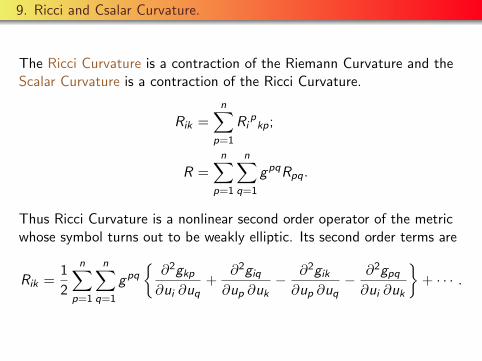
9. Ricci and Csalar Curvature.
The Ricci Curvature is a contraction of the Riemann Curvature and theScalar Curvature is a contraction of the Ricci Curvature.
Rik =n∑
p=1
Ripkp;
R =n∑
p=1
n∑q=1
gpqRpq.
Thus Ricci Curvature is a nonlinear second order operator of the metricwhose symbol turns out to be weakly elliptic. Its second order terms are
Rik =1
2
n∑p=1
n∑q=1
gpq
∂2gkp
∂ui ∂uq+
∂2giq
∂up ∂uk− ∂2gik
∂up ∂uq− ∂2gpq
∂ui ∂uk
+ · · · .

10. Recent Geometric Analysis Solution of Poincare Conjecture.
Figure: Richard Hamilton.
In 1904 Poincare conjecturedthat a closed simply connectedM3 is homeo to the sphere. Thisfollows from Thurston’sGeometrization Conjecture.
In a series of papers beginning 1982,Hamilton perfected PDE machinery tosolve the conjecture. Starting from anyRiemannian metric g0 for M, he evolvedit according to Ricci Flow
∂∂t g = −2Ric(g), g(0) = g0.
Since the solution generally encounterssingularities, he proposed to intervenewith surgery whenever singularitiesform. In 2003, Perelman found a way tocontrol the topology at singularitiesenough to say the flow with surgeryresults in standard topologicalmaneuvers ending at a geometrizablemanifold. Topological methods implythat the original manifold wasgeometrizable.

11. Schematic of Ricci Flow with Surgery.

12. Simplest Example: Heat Equation on the Circle.
The space S1 = R/2πZ is the circle of length 2π. We say that a functionf (θ) ∈ Ck(S1) if f (θ) is defined for all θ ∈ R, is k-times continuouslydifferentiable and is 2π-periodic.
If g(θ) ∈ C(S1) is the initial temperature on a thin unit circular rod. Letu(t, θ) ∈ C2([0,∞)× S1). The temperature for future times satisfies theheat equation
∂u
∂t=
∂2 u
∂θ2, for all t > 0 and θ ∈ S1.
u(0, θ) = g(θ), for all θ ∈ S1.

13. Separation of Variables (Fourier’s Method)
Figure: J. Fourier 1768–1830.
His 1822 Theorie analytique dela chaleur was called “a greatmathematical poem” by Kelvinbut Lagrange, Laplace andLegendre criticized it for alooseness of reasoning.
We make the ansatz that
u(t, θ) = T (t)Θ(θ)
for a 2π-periodic Θ. Heat equationbecomes
T ′(t)Θ(θ) = T (t)Θ′′(θ).
Separating variables implies that there isa constant λ so that
T ′(t)
T (t)= −λ =
Θ′′(θ)
Θ(θ).
This results in two equations
Θ′′ + λΘ = 0, Θ is 2π-periodic on R;
T ′ + λT = 0, for all t > 0.

14. Separate Variables in the Heat Equation.
2π-periodicity of solutions of the first equation imply λ = k2 for k ∈ Z
Θ′′ + λΘ = 0
which yields the solution Θ = A0 if λ = 0 and
Θ(θ) = Ak cos kθ + Bk sin kθ
if λ = k2 for some k ∈ N and constants Ak , Bk .These form a complete basis for L2(S1).The corresponding solution of T ′ + λT = 0 is
T (t) = e−k2t .
Thus, the PDE is solved for k ∈ N by
u(t, θ) = e−k2t (Ak cos kθ + Bk sin kθ) .

15. Separate Variables in the Heat Equation. -
By linearity, the solution is obtained by superposition
u(t, θ) = A0 +∞∑
k=1
e−k2t (Ak cos kθ + Bk sin kθ) . (1)
The initial condition is satisfied
g(θ) = u(0, θ) =1
2A0 +
∞∑k=1
(Ak cos kθ + Bk sin kθ)
if one takes the Fourier coefficients of g(θ). For k ∈ Z+,
Ak =1
π
π∫−π
g(θ) cos kθ dθ, Bk =1
π
π∫−π
g(θ) sin kθ dθ

16. Heat Equation Properties.
Theorem (Heat Equation Properties)
Suppose that g(θ) ∈ C(S1). Then there is a solutionu ∈ C ([0,∞)× S1) ∩ C 2((0,∞)× S1), given by (1), that satisfies theheat equation
ut = uθθ, for (t, θ) ∈ (0,∞)× S1;
u(0, θ) = g(θ), for all θ ∈ S1.
The solution has the following properties:
1 If u and v both satisfy the heat equation, and if u(0, θ) < v(0, θ) forall θ then u(t, θ) ≤ v(t, θ) for all t ≥ 0 and all θ.
2 minS1 g ≤ u ≤ maxS1 g.
3∫
S1(u − 12A0)
2 dθ ≤ e−2t‖g − A0‖22 for all t ≥ 0.
4 There are c1, c2 > 0 so that∫
S1 u2θ dθ ≤ c1e
−2t for all t ≥ c2.
5 u(t, θ) → 12A0 uniformly as t →∞.

17. Maximum Principle. (First Tool to Study Heat Equations.)
Theorem (Maximum Principle for Heat Equation on the Circle)
Suppose that u, v ∈ C([0,T )× S1) ∩ C2((0,T )× S1) both satisfy theheat equation and initial condition
ut = uθθ, vt = vθθ, on (0,T )× S1;
u ≥ v , on 0 × S1.
Thenu ≥ v , on [0,T )× S1.
The idea is that if there is a point (t0, θ0) where solutions first touchu(t0, θ0) = v(t0, θ0) then u(t0, θ) ≥ v(t0, θ) for all θ for all θ. Hence
uθθ(t0, θ0) ≥ vθθ(t0, θ0)
so ut(t0, θ0) ≥ vt(t0, θ0) and the solutions move apart.
However, we can’t draw this conclusion unless the inequalities are strict.

18. Proof of Maximum Principle.
Proof. Choose ε > 0. Let w(t, θ) = u(t, θ)− v(t, θ) + εt + ε. Note thatw satisfies
wt = ut − vt + ε = uθθ − vθθ + ε = wθθ + ε.
At t = 0 we have w(0, θ) > 0. I claim w > 0 for all (t, θ). If not, there isa first time t1 > 0 where w = 0, say at some point w(t1, θ1) = 0.Because w(t, θ1) > 0 for all 0 ≤ t < t1, we have wt(t1, θ1) ≤ 0. Becausew(t1, θ) ≥ 0 for all θ, we have wθθ(t1, θ1) ≥ 0. Plugging into theequation
0 ≥ wt(t1, θ1) = wθθ(t1, θ1) + ε ≥ 0 + ε > 0
which is a contradiction. Thus, w > 0 for all (t, θ), which implies
u(t, θ)− v(t, θ) > −εt − ε.
But for fixed (t, θ), by taking ε > 0 arbitrarily small, it follows that
u(t, θ)− v(t, θ) ≥ 0.

19. Maximum principle. -
To see (2), let
w(t, θ) = minS1
g , v(t, θ) = maxS1
g .
Since w and v are constant, they satisfy the heat equation. Since
w(0, θ) ≤ u(0, θ) ≤ v(0, θ),
it follows from (1) that that for all (t, θ),
w(t, θ) ≤ u(t, θ) ≤ v(t, θ).

20. Integral Estimates. (Second Tool to Study Heat Equations.)
Deduce co-evolution of interesting quantities such as averagetemperature.
To see (3), first notice that the average temperature remains constant intime
d
dt
(1
2π
∫S1
u dθ
)=
1
2π
∫S1
ut dθ =1
2π
∫S1
uθθ dθ = 0.
Thus, for all t ≥ 0,
1
2π
∫S1
u(t, θ) dθ =1
2A0 =
1
2π
∫S1
g(θ) dθ.

21. Co-evolution of Another Quantity: Squared Deviation.
Also the L2 deviation decreases. Using Wirtinger’s inequality
d
dt
∫S1
[u − 1
2A0
]2
dθ = 2
∫S1
[u − 1
2A0
]ut dθ
= 2
∫S1
[u − 1
2A0
]uθθ dθ
= −2
∫S1
u2θ dθ
≤ −2
∫S1
[u − 1
2A0
]2
dθ
This says y ′ ≤ −2y so y ≤ y0e−2t or∫
S1
[u − 1
2A0
]2
dθ ≤
(∫S1
[g(θ)− 1
2A0
]2
dθ
)e−2t .

22. Wirtinger’s Inequality.
Wirtinger’s Inequality bounds the L2 norm of a function by the L2 normof its derivative. It is also known as the Poincare Inequality in higherdimensions. We state stronger hypotheses than necessary.
Figure: Wilhelm Wirtinger1865–1945.
Theorem (Wirtinger’s inequality)
Let f (θ) be a piecewise C1(R) function withperiod 2π (for all θ, f (θ + 2π) = f (θ)). Letf denote the mean value of f
f = 12π
∫ 2π0 f (θ) dθ.
Then∫ 2π0
(f (θ)− f
)2dθ ≤
∫ 2π0 (f ′(θ))2 dθ.
Equality holds iff for some constants a, b,
f (θ) = f + a cos θ + b sin θ.

23. Proof of Wirtinger’s Inequality.
Idea: express f and f ′ in Fourier series. Since f ′ is bounded and f iscontinuous, the Fourier series converges at all θ
f (θ) = a02 +
∑∞k=1 ak cos kθ + bk sin kθ .
Fourier coefficients are determined by formally multiplying by sin mθ orcos mθ and integrating to get
am = 1π
∫ 2π0 f (θ) cos mθ dθ, bm = 1
π
∫ 2π0 f (θ) sinmθ dθ,
hence 2f = a0. Sines and cosines are complete so Parseval equation holds∫ 2π0
(f − f
)2= π
∑∞k=1
(a2k + b2
k
). (2)
Formally, this is the integral of the square of the series, where aftermultiplying out and integrating, terms like
∫cos mθ sin kθ = 0 or∫
cos mθ cos kθ = 0 if m 6= k drop out and terms like∫
sin2 kθ = πcontribute π to the sum.

24. Proof of Wirtinger’s Inequality..
The Fourier Series for the derivative is given by
f ′(θ) ∼∞∑
k=1
−kak sin kθ + kbk cos kθ
Since f ′ is square integrable, Bessel’s inequality gives
π
∞∑k=1
k2(a2k + b2
k
)≤∫ 2π
0(f ′)2. (3)
Wirtinger’s inequality is deduced form (2) and (3) since∫ 2π
0(f ′)2 −
∫ 2π
0
(f − f
)2 ≥ π
∞∑k=2
(k2 − 1)(a2k + b2
k
)≥ 0.
Equality implies that for k ≥ 2, (k2 − 1)(a2k + b2
k
)= 0 so ak = bk = 0,
thus f takes the form f (θ) = f + a cos θ + b sin θ.

25. Co-evolution of interesting quantities: Mean square heat flux.
By differentiating the equation, we get the evolution equation of heatflux uθ
(uθ)t = (ut)θ = (uθθ)θ = (uθ)θθ
L2 norm of heat flux decreases. Using Wirtinger’s inequality
d
dt
∫S1
u2θ dθ = 2
∫S1
uθuθt dθ
= 2
∫S1
uθuθθθ dθ
= −2
∫S1
u2θθdθ
≤ −2
∫S1
u2θdθ
Thus, for any 0 < t0 < t,∫S1
u2θ(t, θ) dθ ≤
(∫S1
u2θ(t0, θ) dθ
)e−2(t−t0).

26. Temperature converges uniformly to its average.
Since θ 7→ u(t, θ) is continuous, there is a point θ0 ∈ S1 such thatu(t, θ0) = 1
2A0 equals its average. Let θ0 ≤ θ1 < θ0 + 2π be any pointon the circle. By Schwarz inequality, for t ≥ c2,
|u(t, θ1)− u(t, θ0)|2 ≤∣∣∣∣∫ θ1
θ0
uθ(t, θ) dθ
∣∣∣∣2≤ (θ1 − θ0)
∫ θ1
θ0
u2θ dθ
≤ 2π
∫S1
u2θdθ
≤ 2πc1e−2t .
Thus temperature converges uniformly because for any θ1 and t ≥ c2,∣∣∣∣u(t, θ1)−1
2A0
∣∣∣∣ ≤ (2πc1)12 e−t .

27. Simplest Geometric Example: How to Round Out a Curve?
Figure: Deform Curve
Is it possible to continuously deforma curve in such a way that
The parts that are bent themost are unbent the fastest;
The curve doesn’t cross itself;
The deformation limits to acircle?
The answer is YES! Method:CURVATURE FLOW HeatEquation! Move curve with normalvelocity proportional to curvature.
Xt = κN.
It turns out
Xt = Xss .

28. Vaughn’s Applet.
Curvature flow applet written by Richard Vaugh, Paradise Valley CC,
http://www.pvc.maricopa.edu/∼vaughn/java/JDF/df.html

28. Vaughn’s Applet.
Curvature flow applet written by Richard Vaugh, Paradise Valley CC,
http://www.pvc.maricopa.edu/∼vaughn/java/JDF/df.html

28. Vaughn’s Applet.
Curvature flow applet written by Richard Vaugh, Paradise Valley CC,
http://www.pvc.maricopa.edu/∼vaughn/java/JDF/df.html

28. Vaughn’s Applet.
Curvature flow applet written by Richard Vaugh, Paradise Valley CC,
http://www.pvc.maricopa.edu/∼vaughn/java/JDF/df.html

28. Vaughn’s Applet.
Curvature flow applet written by Richard Vaugh, Paradise Valley CC,
http://www.pvc.maricopa.edu/∼vaughn/java/JDF/df.html

29. Sethian’s Applet.
Vaughn’s link seems to have disappeared. Here is another.
Curvature flow applets written by James Sethian, University of California,Berkeley.
http : //www.math.berkeley.edu/
∼ sethian/2006/Applets/EvolvingCurves/java curve flow.html

30. Regular Curves
Let X (u) be a regular smooth closed curve in the plane.(Regular means Xu 6= 0.)
X : [0, a] → R2,
X (0) = X (a);
Xu(0) = Xu(a).
The velocity vector is Xu. s is the arclength along the curves(u) = L(X ([0, u]). The speed of the curve is
ds
du= |Xu|
The unit tangent and normal vectors are thus
T =Xu
|Xu|; N = RT = R
(Xu
|Xu|
)where R =
(0 −11 0
)is the 90 rotation matrix.

31. Curvature of a Curve.
The curvature κ measures how fast the unit tangent vector turns relativeto length along the curve.Let θ be the angle of the tangent vector from horizontaL
T = (cos θ, sin θ) so N = RT = (− sin θ, cos θ)
Then the curvature is
κ =dθ
dsso
d
dsT = (− sin θ, cos θ)
dθ
ds= κN
and alsod
dsN = −κT .

32. Curvature of a Circle.
For example, for the circle of radius R,
X (u) = (R cos u,R sin u)
Xu = (−R sin u,R cos u)
ds
du= |Xu| = |(−R sin u,R cos u)| = R
T =(−R sin u,R cos u)
|(−R sin u,R cos u)|= (− sin u, cos u) = (cos θ(u), sin θ(u))
where θ(u) = u +π
2so
κ =dθ
ds=
du
ds
dθ
du=
1
|Xu|· 1 =
1
R.
Equivalently, since N = RT = (− cos u,− sin u),
dT
ds=
du
ds
dT
du=
1
|Xu|(− cos u,− sin u) =
1
RN = κN. so κ =
1
R.

33. Curvature of a Curve.
Note that the derivative of the speed gives
d
du|Xu| =
d
du
√Xu · Xu =
1
2
1
|Xu|2xu · Xuu =
Xu · Xuu
|Xu|.
κ determined from the formula
dT
ds= κN =
1
|Xu|d
du
(Xu
|Xu|
)=
1
|Xu|
(Xuu
|Xu|−
Xuddu |Xu||Xu|2
)
=1
|Xu|
(Xuu
|Xu|− (Xu · Xuu)Xu
|Xu|3
).
By the way, this formula decomposes acceleration into tangential andcentripetal pieces
Xuu =d
du|Xu|T + κ|Xu|2N

34. First Variation of Arclength.
Let’s work out how fast length changes when we perturb the curve.The length L(X ) is obtained from the integral
L0 =
∫Γds =
∫ a
0|Xu| du.
How does the length of Γt given by u 7→ X (t, u) change if we deform thecurve sideways at a velocity v? In a deformation of this kind
∂
∂tX = vN
where v is velocity of deformation and N is the normal to Γt at X (t, u).We seek the first variation of length which is the derivative of L(X ):
Theorem (First Variation of Arclength)
Suppose that X (t, u) is a smooth family of regular closed curves that aredeformed with normal velocity by Xt(t, u) = v(t, u)N(t, u). Then
d
dtL(X ) = −
∫Γt
κv ds. (4)

35. First Variation of Arclength. -
Proof. For arbitrary function g , derivatives with respect to arclength
gs =1
|Xu|gu and ds = |Xu| du
Differentiating,
∂
∂t|Xu| =
Xu · Xut
|Xu|=
Xu · Xtu
|Xu|= T · (Xt)s |Xu|
= T · (vN)s |Xu| = T · (vsN − vκT )|Xu| = −κv |Xu|.
Hence
d
dtL(X ) =
∫∂
∂t|Xu| du = −
∫κv |Xu| du = −
∫κv ds

36. First Variation of Arclength Example.
For example, Y (t, u) =((R − t) cos u, (R − t) sin u
)is a circle of radius
(R − t), N = (cos u, sin u) is the normal for all circles and
dY
dt= −(sin u, cos u) = −N
so v = 1 is constant. Since |Yu| = R − t, ds = (R − t) du and the
curvature of X is κ =1
R − t, the first variation is just
d L
dt= −
∫Γκv ds = −
∫ 2π
0
1
R − t· 1 (R − t)du
= −2π =d
dtL(Y ) =
d
dt2π(R − t).

37. First Variation of Area.
A similar computation gives the first variation of area. WritingX = (x , y), the area A(X ) is obtained from the line integral
A0 =1
2
∮Γx dy − y dx =
1
2
∫ a
0xyu − yxu du =
1
2
∫ a
0RX · Xu du
since RX = (−y , x).
How does the area changes if we deform the curve Γt given by X (t, u)with velocity v in the N direction?The first variation of area is the time derivative of A(X ):
Theorem (First Variation of Area.)
Suppose that X (t, u) is a smooth family of regular closed curves movingsuch that the normal velocity is Xt(t, u) = v(t, u)N(t, u). Then
d
dtA(X ) = −
∫Γt
v ds. (5)

38. First Variation of Area. -
Proof.
d
dtA(Γ) =
1
2
d
dt
∫ a
0RX · Xu du
=1
2
∫ a
0RXt · Xu +RX · Xut du
=1
2
∫ a
0RXt · Xu +RX · Xtu du
=1
2
∫ a
0RXt · Xu −RXu · Xt du
=1
2
∫ a
0
[R(vN) · T −RT · (vN)
]|Xu| du
=1
2
∫ a
0
[−(vT ) · T − N · (vN)
]ds
= −∫ a
0v ds.

39. First Variation of Area Example.
For example, if Y is the circle Y (t, u) =((R − t) cos u, (R − t) sin u
),
dY
dt= −(cos u, cos v) = −N
so v = 1 is constant. Then the first variation is just
dA
dt= −
∫Γ1 ds = −2π(R − t) =
d
dtπ(R − t)2.

40. The Curvature Flow.
Let us assume that we have a family of curves Γt given by X (t, u) fort ≥ 0 and 0 ≤ u ≤ a. If the curve is moving normally at a velocityv(t, u) = κ(t, u), at all points (t, u),
d
dtX (t, u) = κ(t, u)N(t, u),
we say that the family of curves moves by CURVATURE FLOW.
Since Xs = T and Ts = κN, the curvature flow satisfies
Xt = Xss
suggesting that it is a heat equation. Indeed, it is a nonlinear parabolicPDE.BUT, since arclength changes along the flow, this is a nonlinear equation.

41. The Circle Moving by Curvature Flow.
For example, for the family of circles X (t, u) = ρ(t)(cos u, sin u), Thepoints move in the normal direction because
d
dtX = ρ′(t)(cos u, sin u) = −ρ′N
Hence the circles flow by curvature if
−ρ′ = κ =1
ρ
It follows thatρ(t) =
√R2 − 2t
if the initial radius is ρ(0) = R.
The circles shrink and completely vanish when t approaches R2/2.

42. Curvature of Nonparametric Curves.
In the jargon, a curve given by y = f (x) is called nonparametric. It isstill a parameterized curve X (u) = (u, f (u)). Thus
Xu = (1, f ), |Xu| =√
1 + f 2, T =(1, f )√1 + f 2
, N =(−f , 1)√
1 + f 2.
Computing curvature
dT
ds=
1
|Xu|dT
du=
(−f f , f )
(1 + f 2)2=
f
(1 + f 2)32
(−f , 1)√1 + f 2
= κN (6)
so the curvature of a nonparametric curve is
κ =f
(1 + f 2)32

43. Translating Curve Flowing by Curvature.
There is no reason to track individual points of the curve as it flows. Wecould reparameterize as we go and then the trajectory t 7→ X (t, u) neednot be perpendicular to the curve Γt . We need only that the normalprojection of velocity be curvature
N · ∂X
∂t= κ (7)
For example, suppose that a fixed curve moves by steady verticaltranslation. If this is also curvature flow, it is called a soliton. In this case
X =(u, f (u) + ct
), Xu = (1, f ), |Xu| =
√1 + f 2, κ =
f
(1 + f 2)3/2
Then∂X
∂t= (0, c). By (7) the equation for a translation soliton satisfies
c√1 + f 2
=f
(1 + f 2)3/2(8)

44. The Grim Reaper.
The solution of (8) gives asoliton called the GrimReaper. (8) becomes
c =f
1 + f 2=
d
duAtn f
so
Atn f = cu + c1
f = tan(cu + c1)
f = c2 −1
cln cos(cu + c1).
If c = 1 and c1 = c2 = 0,
X (t, u) =(u, t − ln cos(u)
)

45. κN is Independent of Parameterization.
If we change variables according to v = h(u), where h′ is nonvanishing,then
∂
∂v=
∂u
∂v
∂
∂u= h′(v)
∂
∂u.
It follows that
∂
∂s=
1
|Xv |∂
∂v=
h′
|h′Xu|∂
∂u=
ε
|Xu|∂
∂u
where ε = ±1 according to whether h′ > 0 or h′ < 0. Hence Xss is thesame regardless of parameterization.
κN = Xss =1
|Xv |∂
∂v
(1
|Xv |∂
∂vX
)=
1
|Xu|∂
∂u
(1
|Xu|∂
∂uX
).
Note: even the orientation of Γ doesn’t matter.

46. Maximum Principle Prevents Flowing Curve from Touching Itself.
Initially, Γ0 is an embedded curve. The smoothly evolving curve cannoteventually cross itself at distinct points because if they would ever touch,their motion would tend to separate the points.
Suppose at some t0 > 0 the evolving curve first touches at two pointsu1 6= u2 but X (t0, u1) = X (t0, u2). The touch from inside Γ as if theenclosed region is pinched or from the outside as if the regions bendtogether.

47. Maximum Principle Prevents Flowing Curve from Touching Itself. -
Figure: At Instant of Touching
Let us call Y (t, u) the flow X near(t0, u1) and Z (t, u) the flow X near(t0, u2). Represent both curvesnonparametrivally as graphs over thesame variable
Y (t, v) = (v , f (t, v)),
Z (t, v) = (v , g(t, v)).
Suppose that f (t0, v0) = g(t0, v0)and f (t1, v) ≤ g(t1, v) for v near v0
as would be the case at the instantof the first interior touch. It followsthat
fv (t0, v0) = gv (t0, v0)
fvv (t0, v0) ≤ gvv (t0, v0)

48. Maximum Principle Prevents Flowing Curve from Touching Itself. - -
It follows from (6) that the flow velocity
Yss = fvv(−fv , 1)
(1 + f 2v )2
Zss = gvv(−gv , 1)
(1 + g2v )2
Since the vectors are equal at (t0, v0) since fv (t0, v0) = gv (t0, v0).
Because fvv (t0, v0) ≤ gvv (t0, v0), the upper curve is moving faster upwardthan the lower curve: the curves tend to move apart!
This idea can be turned into a proof.

49. Closed Curves Flowing by Curvature Vanish in Finite Time.
The same argument says that if one curve starts inside another, thenthey never touch as they flow. Thus the inside blob must extinguishbefore the shrinking disk does!
Figure: Flowing inside curve vanishes before the outside curve vanishes.
Also, closed curves inside the Grim Reaper die before it sweeps by!

50. Flow Shrinks Curves via Integral Estimate.
Let us assume that Γt are embedded closed curves on the intervalt ∈ I = [0,T ). Then the first variation formula (4), (5) tells us that thearea and length shrink.Under curvature flow, the normal velocity is v = κ. Thus at each instantt ∈ I we have
dL
dt= −
∫Γt
κ2 ds,
dA
dt= −
∫Γt
κ ds = −2π.
The latter integral is the total turning angle (= 2π) of an embeddedclosed curve. It follows that
A(Γt) = A0 − 2πt
where A0 = A(Γ0) is the area enclosed by the starting curve.
The flow can only exist up to vanishing time T =A0
2π.

51. Inradius / Circumradius
Let K be the region bounded by γ. The radius of the smallest circulardisk containing K is called the circumradius, denoted Rout. The radius ofthe largest circular disk contained in K is the inradius.
Rin = supr : there is p ∈ E2 such that Br (p) ⊆ KRout = infr : there exists p ∈ E2 such that K ⊆ Br (p)
Figure: The disks realizing the circumradius, Rout, and inradius, Rin, of K .

52. Bonnesen’s Inequality.
Figure: T. Bonnesen 1873–1935
Theorem (Bonnesen’s Inequality[1921])
Let Ω be a convex plane domainwhose boundary has length L andwhose area is A. Let Rin and Rout
denote the inradius andcircumradius of the region Ω. Then
rL ≥ A + πr2 (9)
for all Rin ≤ r ≤ Rout.

53. Proof of Bonnesen’s Inequality.
It suffices to show (9) for polygons Pn and for Rin < r < Rout and thenpass (9) to the limit as Pn → Ω. Let Br (x , y) be the closed disk ofradius r and center (x , y). Let Er denote the set of centers whose ballstouch Pn.
Er =(x , y) ∈ R2 : Br (x , y) ∩ Pn 6= ∅
Let n(x , y) denote the number of points in ∂Br (x , y) ∩ ∂Pn. Thetheorem follows by computing
I =
∫Er
n(x , y) dx dy
in two ways.
Since Br (x , y) can neither contain, nor be contained by Pn, except on aset of measure zero, n is finite and
n(x , y) ≥ 2 for almost all (x , y) ∈ Er .

54. Area of Er for Polygons.
Hence Er consists of all points in the interior of Pn as well as all pointswithin a distance r .
Figure: Er of polygon has area A(Pn) + L(∂Pn)r + πr2.
Thus2A + 2Lr + 2πr2 ≤ I .

55. Measure of points touching a single boundary segment.
It follows from Rin < r < Rout that Br touches Pn if and only if ittouches ∂Pn. Let σ be one of the boundary line segments. Let nσ(x , y)be the number of points in σ ∩ ∂Br (x , y). The set Iσ of centers of circlestouching σ is the union of circles with centers on σ.
∫σ∩∂Br (x ,y) 6=∅
nσ dx dy = 4r L(σ).

56. Proof of Bonnesen’s Inequality. -
Hence
I =
∫Er
n dx dy =∑
σ
∫σ∩Br (x ,y) 6=∅
nσ dx dy =∑
σ
4r L(σ) = 4r L(∂Pn).
Putting both computations together
2A + 2Lr + 2πr2 ≤ I ≤ 4rL
or (9),A + πr2 ≤ rL.

57. Support Function.
The distance of the tangent line to the origin is called the supportfunction
p = −X · N = −X · RXu
|Xu|.
Hence, the area is
A = −1
2
∫ΓX · RXu du =
1
2
∫Γp ds
The length is
L =
∫ΓT ·T ds =
∫ΓT ·Xs ds = −
∫ΓTs ·X ds = −
∫ΓκN ·X ds =
∫Γκp ds

58. Domains get Rounder under Curvature Flow.
Figure: M. Gage
Theorem (Gage’s Inequality [1983])
Let Ω be a C2 convex plane domain whoseboundary Γ has length L and whose area is A.Then
πL
A≤∫
Γκ2 ds. (10)
Proof. By Schwarz’s Inequality,
L2 =
(∫Γκp ds
)2
≤∫
Γκ2ds
∫Γp2 ds
(10) follows if Ω can be moved so∫Γp2 ds ≤ AL
π. (11)

59. Proof of Gage’s Inequality.
Proof. First we assume Ω is symmetric about the origin. Then
Rin ≤ p ≤ Rout.
Integrate Bonnesen’s Inequality
L
∫Γp ds ≥ A
∫Γ
ds + π
∫Γp2 ds
2AL ≥ AL + π
∫Γp2 ds
which is (11) for symmetric domains.Now assume Ω is any convex domain. We claim that Ω can be bisectedby a line that divides the area into equal parts and cuts both boundarypoints at parallel tangents.

60. Proof of Gage’s Inequality. -
The claim depends on the Intermediate Value Theorem. Let g(s) be thecontinuous function such that s < g(s) < s + L which gives the placealong Γ such that the line through the points X (s) and X (g(s)) bisectsthe area. Hence g(g(s)) = s + L. Consider the continuous function
h(s) =[T (s)× T (g(s))
]· Z
where Z is the positively oriented normal to the plane. h(s) = 0 iffT (s) = −T (g(s)).Observe h(0) = −h(g(0)). If h(0) = 0 then s0 = 0 determines the line.Otherwise, by IVT, there is an s0 ∈ (0, g(0)) where h(s0) = 0 and s0determines the line.
Let L be the line segment from X (s0) to X (g(s0)). Move the curve sothe midpoint of L is the origin.
Let γ1 and γ2 be the sides of Γ split by L.

61. Proof of Gage’s Inequality. - -
Figure: Cut and Reglue along Line L that Halves the Area and Touches theCurve at Parallel Tangents.

62. Proof of Gage’s Inequality. - - -
Erasing γ2 for the moment, reflect γ1 through the origin to form aclosed, convex curve, that is symmetric with respect to the origin. Notethat the tangents at the endpoints of γ1 must be parallel for γ1 ∪ (−γ1)to be convex. We apply (11)
2
∫γ1
p2 ds ≤ 2AL1
π.
where 2L1 is the length of γ1 ∪ (−γ1). Similarly with γ2 ∪ (−γ2),
2
∫γ2
p2 ds ≤ 2AL2
π.
Adding these two inequalities yields
2
∫Γp2 ds ≤ 2AL1 + 2LA2
π=
2AL
π
which is (11) for general convex domains.

63. Convex Curves get Rounder as they Flow.
For any closed curve, the isoperimetric inequality says that the boundarycannot be shorter than that of a circle with the same area
L2 ≥ 4πA.
Theorem (Gage [1983])
Let Γt be a C2 family of curves flowing by curvature Xt = Xss for0 ≤ t < T starting from a convex Γ0. Then
1 The isoperimetric ratio decreases: ddt
(L2
4πA
)≤ 0.
2 If the flow survives until T = 12πA0 (it does by the Gage and
Hamilton Theorem) and A → 0 as t → T, then
L2
4πA → 1 as t → T.
Hence, the curves become circular in the sense that
(Rout(t)−Rin(t))2
4R2out
≤ L2
4πA − 1 → 0

64. Decrease of Isoperimetric Ratio.
(1) is a computation with the first variation formulas and Gage’sInequality
d
dt
(L2
4πA
)=
2ALL′ − L2A′
4πA2
=L
2πA
(−∫
Γt
κ2 ds +πL
A
)≤ 0.
(2) is similar, using a stronger form of Gage’s Inequlity.
(3) follows from a the Strong Isoperimetric Inequality of Bonnesenand A ≤ πR2
out
π2 (Rout(t)− Rin(t))2
4π2R2out
≤ L2 − 4πA
4πA=
L2
4πA− 1.

65. Strong Isoperimetric Inequality of Bonnesen.
Theorem (Strong Isoperimetric Inequality of Bonnesen)
Let Ω be a convex planar domain with boundary length L and area A.Let Rin and Rout denote the inradius and circumradius of the Ω. Then
L2 − 4πA ≥ π2(Rout − Rin)2. (12)
Proof. Consider the quadratic function f (s) = πs2 − Ls + A. ByBonnesen’s inequality, f (s) ≤ 0 for all Rin ≤ s ≤ Rout. Hence thesenumbers are located between the zeros of f (s), namely
Rout ≤L +
√L2 − 4πA
2π
L−√
L2 − 4πA
2π≤ Rin.
Subtracting these inequalities gives
Rout − Rin ≤√
L2 − 4πA
π,
which is (12).

66. Curvature Flow Properties.
Theorem (M. Gage & R. Hamilton [1986], M. Grayson [1987])
Suppose that Γ0 ∈ C2 is an embedded curve in the plane with boundedcurvature and encloses area A0. Then there is a unique smooth family ofembedded curves independent of parametrization Γt that satisfiesXt = Xss on [0,T∞), where T∞ = 1
2πA0. The solution has the followingproperties:
1 If Γ0 is nonconvex, there is a time t1 ∈ (0,T∞) where Γt1 is convex.
2 If Γt1 is ever convex but possibly with straight line segments, then Γt
will be strictly convex for t > t1.3 The flow shrinks to a round point in the sense that
Rin
Rout→ 1 as t → T∞;
minΓt κ
maxΓt κ→ 1 as t → T∞;
Curvature stays bounded on compact intervals [0,T∞ − ε];maxΓt |∂α
θ κ| → 0 as t → T∞ for all α ≥ 1, where T = (cos θ, sin θ).

67. Commuting Derivatives.
Theorem
Let Γt be a C2 family of curves flowing by curvature Xt = Xss fort ∈ [0,T ). Then
1 If g(t, u) ∈ C2 is any function, then gst = gts + κ2gs ;
2 Tt = κsN and Nt = −κsT;
3 κt = κss + κ3.
Compute (1) using gtu = gut and Xtu = Xut (but gst 6= gts):
gst =
(gu
|Xu|
)t
=gtu
|Xu|− Xu · Xtu
|Xu|3gu
= gts − T · (Xt)s gs
= gts − T · (κN)s gs
= gts − T · (κsN − κ2T ) gs
= gts + κ2gs .

68. I’m Never Happier than when I’m Differentiating!
To see (2a), use (1) and Xt = κN,
Tt = Xst = Xts + κ2Xs = (κN)s + κ2T = κsN − κ2T + κ2T = κsN.
To see (2b), as the rotation R doesn’t depend on t,
Nt = (RT )t = R(Tt) = R(κsN) = −κsT .
Finally, to see (3), differentiate the defining equation for curvatureTs = κN, using (2b)
Tst = (κN)t = κtN + κNt = κtN − κκsT
Then using (1) and (2a)
Tst = Tts + κ2Ts = (κsN)s + κ3N = κssN − κκsT + κ3N.
Equating gives (3)κt = κss + κ3.

69. Convex curves stay convex.
Corollary
Let Γt be a C2 family of curves flowing by curvature Xt = Xss fort ∈ [0,T ). Suppose that Γ0 is convex. Then Γt is convex for allt ∈ [0,T ).
Proof idea. The curve is convex iff it’s curvature is nonnegative. Henceκ(0, s) ≥ 0 for all s. Apply the maximum principle to κ which satisfies
κt = κss + κ3.
If t0 ∈ [0,T ) is the first time κ is zero, say at s0, then we have
κ(t0, s0) = 0 and κ(t0, s) ≥ 0 for all s.
Thus κss(t0, s0) ≥ 0 and
κt(t0, s0) = κss(t0, s0) + κ3(t0, s0) ≥ 0 + 0
so the curvature is increasing and cannot dip below the x-axis.

70. Mean Curvature Flow Properties.
Theorem (G. Huisken, [1984].)
Suppose that Mn0 ⊂ Rn+1 is a C2 embedded closed convex hypersurface
in Euclidean Space with bounded curvature. Then there is a uniquesmooth family of embedded hypersurfaces, independent ofparametrization, Mt , that satisfy Xt = ∆X = nHN on a maximal interval[0,T∞). The solution has the following properties:
1 Mt will be strictly convex for t > 0.2 The flow shrinks to a round point in the sense that
Rin
Rout→ 1 as t → T∞;
minΓt κ1
maxΓt κn→ 1 as t → T∞, where the κ1 ≤ · · · ≤ κn are principal
curvatures of Mt (eigenvalues of the second fundamental form hij .);The principal curvatures stay bounded on compact intervals[0,T∞ − ε];maxΓt |∂α
θ hij | → 0 as t → T∞ for all α ≥ 1, where θ = N ∈ Sn.

71. Ricci Flow Properties.
Theorem (R. Hamilton, [1982].)
Suppose that (Mn0 , g0) be a smooth compact Riemannian Manifold (thus
g0 is a metric with bounded sectional curvature). Then there is a uniquesmooth family of metrics gt , that satisfy
gt = −2 Ric(g)
on a maximal interval [0,T∞). The solution has the following properties:
1 If (M3, g0) has positive sectional curvature, then it will have positivecurvature for t > 0. (Same for Ricci Curvature.)
2 The flow shrinks to a manifold of constant positive sectionalcurvature in the sense that
minΓt Sect(g)
maxΓt Sect(g)→ 1 as t → T∞, where the Sect(g) is the sectional
curvature of g ;The sectional curvatures stay bounded on compact intervals[0,T∞ − ε];maxΓt (T − t) |∇αRiem(g)| → 0 as t → T∞ for all α ≥ 1.

Thanks!