Heads Up - Deloitte

NUMERICAL LINEAR ALGEBRA WITH APPLICATIONSNumer. Linear Algebra Appl. 2008; 15:755–777Published online in Wiley InterScience (www.interscience.wiley.com). DOI: 10.1002/nla.622

Numerical solution of large-scale Lyapunov equations, Riccatiequations, and linear-quadratic optimal control problems

Peter Benner1,∗,†,‡, Jing-Rebecca Li2,§ and Thilo Penzl3,¶

1Fakultat fur Mathematik, TU Chemnitz, 09107 Chemnitz, Germany2INRIA-Rocquencourt, Projet POEMS, Domaine de Voluceau–Rocquencourt–B.P. 105,

78153 Le Chesnay Cedex, France3Last address: Department of Mathematics and Statistics, University of Calgary, Calgary, Alta., Canada T2N 1N4

SUMMARY

We study large-scale, continuous-time linear time-invariant control systems with a sparse or structuredstate matrix and a relatively small number of inputs and outputs. The main contributions of this paperare numerical algorithms for the solution of large algebraic Lyapunov and Riccati equations and linear-quadratic optimal control problems, which arise from such systems. First, we review an alternatingdirection implicit iteration-based method to compute approximate low-rank Cholesky factors of the solutionmatrix of large-scale Lyapunov equations, and we propose a refined version of this algorithm. Second, acombination of this method with a variant of Newton’s method (in this context also called Kleinmaniteration) results in an algorithm for the solution of large-scale Riccati equations. Third, we describe animplicit version of this algorithm for the solution of linear-quadratic optimal control problems, whichcomputes the feedback directly without solving the underlying algebraic Riccati equation explicitly. Ouralgorithms are efficient with respect to both memory and computation. In particular, they can be appliedto problems of very large scale, where square, dense matrices of the system order cannot be stored in thecomputer memory. We study the performance of our algorithms in numerical experiments. Copyright q2008 John Wiley & Sons, Ltd.

Received 5 January 2008; Revised 18 July 2008; Accepted 22 July 2008

KEY WORDS: Lyapunov equation; algebraic Riccati equation; linear-quadratic optimal control; LQRproblem; Newton’s method; low-rank approximation; control system; sparse matrices

∗Correspondence to: Peter Benner, Fakultat fur Mathematik, TU Chemnitz, 09107 Chemnitz, Germany.†E-mail: [email protected]‡This author’s part of the work was completed while he was with the Department of Mathematics, University ofBremen, Germany.§This author’s part of the work was completed while she was with the Department of Mathematics, MIT, Cambridge,MA, U.S.A.¶Thilo Penzl (28/06/1968–17/12/1999) was supported by DAAD (Deutscher Akademischer Austauschdienst), Bonn,Germany.

Copyright q 2008 John Wiley & Sons, Ltd.

756 P. BENNER, J.-R. LI AND T. PENZL

PREAMBLE

This is an unabridged reprint of an unpublished manuscript written by the authors in 1999. Thelatest version of this work was finalized on December 8, 1999. Thilo Penzl died in a tragicavalanche accident on December 17, 1999, in Canada, and thus, work on the manuscript came to anabrupt end. Nevertheless, this work was often cited and requested by people working on large-scalematrix equations as it forms the basis for parts of the software package LyaPack [1]. This specialissue on Large-Scale Matrix Equations of Special Type offered the possibility to make this draftavailable in the open literature. Due to this fact, we did not take into account any developmentsince 2000 except for updated references. Most changes regarding the original manuscript, in largeparts prepared by Thilo Penzl shortly before his sudden death, are to be found in some re-wordingand corrections of grammar and typos. Sometimes, we add a footnote if a statement in the originaldraft is no longer (completely) true due to recent developments. We hope that this publication ofthe manuscript serves the community and helps to bear in remembrance the influential scientificwork Thilo Penzl contributed in his by way too short career.

1. INTRODUCTION

Continuous-time, finite-dimensional, linear time-invariant (LTI), dynamical systems play an essen-tial role in modern control theory. In this paper we deal with state–space realizations

x(�) = Ax(�)+Bu(�), x(0)= x0

y(�) = Cx(�)(1)

of such systems. Here, A∈Rn,n , B∈Rn,m , C ∈Rq,n , and �∈R. (Throughout this paper, R, Rn,m ,C, Cn,m denote the sets of real numbers, real n×m matrices, complex numbers, and complexn×m matrices, respectively.) The vector-valued functions u, x , and y are called input, state, andoutput of the LTI system (1), respectively. The order of this LTI system is n. Typically, n�m,q .

In the last 2–3 decades, much research has addressed the construction of numerically robustalgorithms for a variety of problems that arise in context with linear systems as in (1). Suchproblems are, for example, optimal control, robust control, system identification, game theory,model reduction, and filtering, see e.g. [2–6]. However, these methods generally have at least amemory complexity O(n2) and a computational complexity O(n3), regardless whether or not thesystem matrix A is sparse or otherwise structured. Therefore, the majority of numerical algorithmsin linear control theory is restricted to systems of moderate order. Of course, the upper limit for thisorder depends on the problem to be solved as well as the particular computing environment and mayvary between a few hundreds and a few thousands. However, a significant number of applicationslead to dynamical systems of larger order. Large systems arise from the semidiscretization of(possibly linearized) partial differential equations (PDEs) by means of finite differences or finiteelements, see e.g. [7–10], and many more. Another source for such systems is circuit designand simulation (VLSI computer-aided design, RCL interconnect modeling, etc.) [11, 12]. Furtherexamples include, for instance, large mechanical space structures [13, 14].

Mostly, systems originating from the applications mentioned above possess two interesting prop-erties. First, their order n is large (say, n>1000), but the dimensions of the input and output spacesare relatively small (m,q�n, often m,q�10). For example, the order of a system arising from a

Copyright q 2008 John Wiley & Sons, Ltd. Numer. Linear Algebra Appl. 2008; 15:755–777DOI: 10.1002/nla

NUMERICAL SOLUTION OF LARGE-SCALE LYAPUNOV AND RICCATI EQUATIONS 757

parabolic PDE is about the number of grid points or mesh nodes used for the semidiscretization,which is relatively large. In contrast, m and q are often quite small and independent of the finenessof the discretization. Second, the system matrix A is structured. Often, A is a sparse matrix orit is implicitly represented as a product of sparse matrices and inverses of sparse matrices. Ingeneral, this structure allows the numerically inexpensive realization of matrix-vector products andthe efficient solution of systems of linear equations with A. The smallness of m and q and thestructure of A are most important for the usefulness of the algorithms we will present.

Basically, this paper contains three contributions which are algorithms for large continuous-timealgebraic Lyapunov equations (CALEs), continuous-time algebraic Riccati equations (CAREs),and linear-quadratic optimal control problems. Among the latter problem class, we will specificallybe concerned with the problem commonly known as linear-quadratic regulator problem in controltheory, see e.g. [3, 9, 15, 16]. We therefore use the common abbreviation LQR problem whenaddressing it. We will solve large CALEs by a method based on the well-known alternatingdirection implicit (ADI) iteration. The basic version of this method has been proposed before,but here we present an improved algorithm and discuss numerical aspects in more detail. Thereexist plenty of applications for CALEs, one of which is the solution of CAREs. We will combineNewton’s method with the ADI-based CALE solver to compute efficiently the stabilizing solutionof large CAREs. Among many other applications in control theory, LQR problems can be solvedby computing the solution of CAREs. An implicit version of our combined algorithm (similar toan algorithm proposed in [17]) will be used to solve LQR problems in a more memory efficientway without forming CARE solutions.

This paper is organized as follows. For the ease of exposition, we will introduce the problemsaddressed in it in reverse order. We describe the basics of the LQR problem in Section 2 and theclassical Newton method for CAREs in Section 3. In Section 4 ,we discuss the efficient solution oflarge CALEs by the ADI-based method. The combination of this method with the Newton iterationfor CAREs is proposed in Section 5, whereas the implicit formulation of the resulting algorithmis presented in Section 6. The results of numerical experiments with our algorithms are reportedin Section 7. Finally, concluding remarks are provided in Section 8.

2. THE LINEAR-QUADRATIC OPTIMAL CONTROL PROBLEM

Consider the linear-quadratic optimal control problem (referred to as LQR problem in the followingas explained above), where the cost functional

J(u, y, x0)= 1

2

∫ ∞0

y(�)TQy(�)+u(�)TRu(�)d� (2)

with

Q=QT�0 and R= RT>0 (3)

is to be minimized and the LTI system (1) represents the constraints. The solution of this problemis determined by the linear state feedback

u(�)=−R−1BTX∗x(�)=:−KT∗ x(�) (4)



where X∗ is the symmetric, positive semidefinite, stabilizing solution of the CARE

R(X)=CTQC+ATX+X A−XBR−1BTX=0 (5)

e.g. [4, 6]. A solution X of this CARE is called stabilizing iff the closed-loop matrix A−BR−1BTXis stable. We call a matrix stable iff each of its eigenvalues has a negative real part. Under moderateassumptions a unique stabilizing solution of (5) exists, see e.g. [2, 16]. The transpose of the matrixK∗ defined by (4) is called optimal state feedback.

The CARE offers a possibility to solve the LQR problem analytically using (4). Of course, thisis only feasible for very small dimension n. Therefore, usually the computation of the optimalcontrol involves the numerical solution of the CARE (5). Many methods for this purpose havebeen devised since the occurrence of the CARE in the solution of the LQR problem in the early60s [18]. We will give a brief survey on the usual approaches in the next section. But of course,there are other possibilities to solve the LQR problem:

1. Solve it as constrained optimization problem. This requires to discretize the integral expres-sion as well as the differential equation and to form a quadratic program, which can then besolved by any method feasible for quadratic programming.

2. Using either Pontryagin’s maximum principle or a direct proof based on the calculus ofvariations (see e.g. [4, 19] and references therein), it can be shown that the optimal controland the associated trajectory can be obtained from the two-point boundary value problem

[x(t)

�(t)

]=

[A BR−1BT

CTQC −AT

][x(t)

�(t)

],

x(0)= x0

limt→∞�(t)=0 (6)

where �(t) is called the co-state of the system and the optimal control is obtained from �as u(t)= R−1BT�(t). This offers the possibility to solve the LQR problem using numericalmethods for linear boundary value problems.

Both these approaches involve a discretization error. Moreover, the infinite time interval needs tobe truncated and it is difficult to define a suitable interval [0,T ] so that an accurate solution isobtained in a reasonable time. Another difficulty with the Approach 1 is the enormous size of theresulting quadratic program due to the discretization of the cost functional (2) and the differentialequation (1), see also [20] for more details on this approach. Another advantage of the solutionvia the CARE is the feedback form (4) of the optimal control. In contrast to the solutions obtainedby the other two approaches, this allows the direct implementation as a controller in a closed-loopcontrol system.

3. NEWTON’S METHOD FOR ALGEBRAIC RICCATI EQUATIONS

The numerical solution of CAREs of the form (5) is the central task in solving optimal controlor optimization problems for linear continuous-time systems, such as stabilization, LQR prob-lems, Kalman filtering, linear-quadratic Gaussian control, H2 optimal control, etc.; see e.g.[4, 6, 15, 16, 21] and the references given therein. We will assume here that Q is positive semidef-inite and R is positive definite and that a unique stabilizing solution of (5) exists. Note that the



methods to be considered here rely on these assumptions as we make use of the fact that theright-hand side in the equivalent formulation of (5),

(A−BR−1BTX)TX+X (A−BR−1BTX)=−CTQC−XBR−1BTX (7)

is positive semidefinite. CAREs as they occur in model reduction [22, 23] or H∞ (sub-) optimalcontrol [24–26] differ from (5) in that the right-hand side in (7) is in general indefinite. Therefore,these CAREs cannot be treated directly by the methods presented in this paper.

We are interested in solving (5) for large and structured coefficient matrices A and low-rankmatrices S and G. The usual solution methods for CAREs such as the Schur vector method [27],the sign function method [28–30], or symplectic methods [31–33] do not make (full) use of thesestructures and require O(n3) flops and workspace of size O(n2) even for sparse problems, andare therefore not suitable for our purpose. (For surveys of the most popular approaches with cubiccomplexity, see [3–6, 34].)

All the methods mentioned above use the corresponding Hamiltonian eigenvalue problem tosolve (5). Methods that exploit the sparsity in the Hamiltonian matrix are proposed in [35, 36]. Therethe Hamiltonian matrix is projected onto a reduced-order Hamiltonian for which the correspondingCARE of reduced size is solved. This solution is then prolongated to a full-size Riccati solutionmatrix. Similarly, low-rank methods that are based on the projection of the underlying LTI systemonto a reduced-order model can be found in [37, 38]. Usually, these projections are computedusing a Krylov subspace method. No convergence theory for these methods is known and often,small residuals can only be obtained with these approaches for relatively large ‘reduced-order’systems.

Another approach to solve CAREs is to treat them as systems of nonlinear equations. It is thenstraightforward to use Newton’s method or its relatives [39–42] for its solution. As the Newtoniteration (see Algorithms 1 and 2 below) consists of solving a sequence of Lyapunov equations, itcan be used to solve large-scale problems if efficient methods for solving large Lyapunov equationsare available. This idea has been used in [17, 43, 44]. The methods there rely on the implementationof an accelerated Smith iteration or a block SOR method for the Lyapunov equation. Althoughthe methods in [43, 44] explicitly rely on the specific structure of the underlying control problem,the method in [17] can be considered as a general-purpose solver for computing the optimal statefeedback in large and sparse LQR problems. This latter method has some close relations to themethod that will be developed in this paper. We discuss these relations and the differences inSection 6.

Our methods make use of a factorization T T T=CTQC+XBR−1BTX , where T ∈Rn×t witht�n and the fact that in this case, the solution of the CARE can be approximated by a productZ ZT of low rank.‖Similar approaches have been used to compute a factored solution of the CARE in [23, 45].

Both approaches use Hammarling’s method [46] for solving the Lyapunov equations during theiteration steps of Newton’s method. The method for solving Lyapunov equations suggested in[46] works with the n×n Cholesky factors of the solution and never forms the full solutionmatrix. Nevertheless, the use of the QR algorithm, as initial step in this approach, requires dense

‖It turns out that in some situations, we will have to use complex arithmetic so that the approximate CARE solutionwill have the form Z ZH , where ZH denotes the conjugate complex transpose of Z .



Algorithm 1. (Newton’s method for the CARE (5))

INPUT: A, B, C , Q, R as in (5) and a starting guess X (0).

OUTPUT: An approximate solution X (k) of (5).

FOR k=1,2, . . . ,K (i−1)= X (k−1)BR−1.Solve

(AT−K (k−1)BT)N (k)+N (k)(A−BK (k−1)T)=−R(X (k−1))

for N (k).

X (k)= X (k−1)+N (k).

(8)

END

Algorithm 2. (Newton’s method for the CARE (5)—Kleinman iteration)

INPUT: A, B, C , Q, R as in (5) and a starting guess K (0) for the feedback matrix.

OUTPUT: An approximate solution X (k) of (5) and an approximation K (k) of the optimal state feedback.

FOR k=1,2, . . . ,Solve

(AT−K (k−1)BT)X (k)+X (k)(A−BK (k−1)T)=−CTQC−K (k−1)RK (k−1)T

for X (k).

K (k)= X (k)BR−1.

(9)

END

matrix algebra at a cost of O(n3) flops and O(n2) memory and is therefore not suitable for ourpurpose.

In the remainder of this section we review Newton’s method for the special form of the CAREgiven in (5). Throughout this paper we use superscripts in parentheses to label variables withinthe Newton iteration.

There are two possible formulations of Newton’s method for CAREs. The first one (Algorithm 1)can be considered as the standard formulation of Newton’s method applied to a system of nonlinearequations. The formulation of Newton’s method proposed by Kleinman [41] (see Algorithm 2)is one of the standard methods for computing the stabilizing solution of the CARE (5). It isbased on (7).

Both formulations are mathematically equivalent. If K (0) is identical in both implementations,i.e. if in Algorithm 2, K (0)= X (0)BR−1, then they deliver the same sequences of X (k)’s and K (k)’s.The following theorem summarizes the convergence theory for Algorithms 1 and 2.



Theorem 1If (A, B) is stabilizable, i.e. rank [A−�In, B]=n for all �∈C with non-negative real part, then

choosing X (0)= X (0)T∈Rn×n in Algorithm 1 or K (0)∈Rn×m in Algorithm 2, such that A−BK (0)T

is stable, the iterates X (k) and K (k) satisfy the following assertions:

(a) For all k�0, the matrix A−BK (k)T is stable and the Lyapunov equations (8) and (9) admitunique solutions, which are positive semidefinite.

(b) {X (k)}∞k=1 is a non-increasing sequence, satisfying X (k)�X (k+1)�0 for all k�1. Moreover,X∗= limk→∞ X (k) exists and is the unique stabilizing solution of the CARE (5).

(c) There exists a constant �>0, such that

‖X (k+1)−X∗‖��‖X (k)−X∗‖2, k�1

i.e. the X (k) converge globally quadratic to X∗ from any stabilizing initial guess.

A complete proof of the above result can be found, e.g. in [16].Though Algorithms 1 and 2 look very similar, there are some subtle differences, which play a

fundamental role in their implementation for large-scale structured systems.The main disadvantage of Algorithm 1 is that the right-hand side of the CALE (8) is the

residual of the CARE, which is in general an indefinite, full-rank matrix. As the performance ofthe CALE solver that will be used in this paper strongly depends on the low-rank structure of theright-hand side, the formulation of Algorithm 2 is preferable as the right-hand side of the CALE(9) has rank at most m+q . Moreover, if the solution of (9) is computed by a low-rank method likethe method presented in Section 4, yielding a low-rank solution of the CALE, the approximatesolutions of the CARE computed by Algorithm 2 themselves will be of low rank. This cannot beguaranteed for Algorithm 1 as there, the low-rank solution of the CALE is added to the last iteratesuch that in general, the rank of the iterates computed this way will be increasing. Moreover, forinitialization, a stabilizing symmetric matrix X (0)∈Rn,n is needed in Algorithm 1, whereas onlya stabilizing feedback K (0)∈Rn,m is needed in Algorithm 2. Starting from K (0) is in particularfavorable for problems, where m�n and the implicit version of Newton’s method, computing anapproximation to K∗ as presented in Section 6, is to be used. For these reasons, in this paper weexclusively use implementations of Newton’s method for CAREs based on the formulation given inAlgorithm 2.

Remark 2The computation of a stabilizing initial guess X (0) or feedback K (0), respectively, is a computationalchallenge by itself if A is not stable—otherwise, i.e. if all eigenvalues of A have negative realpart, one can simply use X (0)=0 or K (0)=0. Stability of A can often be assumed in applicationsarising from parabolic PDEs, so that for a large class of practical applications, we do not need tocompute stabilizing initial guesses or feedbacks. In case we have to find a stabilizing X (0) or K (0),one can follow the approach taken in [17] based on Chandrasekhar’s method. For small, densesystems (partial) stabilization techniques based on solving a Lyapunov equation or pole placementhave been suggested, see e.g. [3, 6] and references therein. It is an open problem to extend thesemethods to large and sparse systems. We will not discuss this any further in this paper.

In the following section, we discuss methods for solving the Lyapunov equations arising in eachNewton step of Algorithms 1 and 2.



4. SOLUTION OF LARGE LYAPUNOV EQUATIONS

Besides Newton’s method for CAREs, several topics in control theory, such as stability analysis,stabilization, balancing, and model reduction involve CALEs; see e.g. [47–50]. These linear matrixequations usually have the structure

FX+XFT=−GGT (10)

where G∈Rn,t is a rectangular matrix with t�n and the matrix F ∈Rn,n is stable. The stabilityof F is sufficient for the existence of a solution matrix X ∈Rn,n , which is unique, symmetric, andpositive semidefinite. If the pair (F,G) is controllable, then X is even positive definite. Theseand other theoretical results on CALEs can be found in [51, 52], for example. Note that (10) ismathematically equivalent to a system of linear equations with O(n2) unknowns. For this reason,CALEs of order n>1000 are said to be of large scale.

The Bartels–Stewart method [53] and Hammarling’s method [45] are the numerical standardmethods for CALEs. While the first is applicable to the more general Sylvester equation, thesecond tends to deliver more accurate results in the presence of round-off errors. Both methodsrequire the computation of the Schur form of F . As a consequence, they generally cannot profitfrom sparsity or other structures in the equation. The squared Smith method [54] and the signfunction method [30] are iterative methods, which cannot exploit sparsity or structures as well.∗∗However, they are of particular interest when dense CALEs are to be solved on parallel computers[57, 58].

ADI [59, 60] is an iterative method, which often delivers good results for sparse or structuredCALEs. The solution methods mentioned so far have the computational complexity O(n3), exceptfor the ADI method. Its complexity strongly depends on the structure of F and can be muchlower. All methods have the memory complexity O(n2) because they generate the dense solutionmatrix X explicitly. It should be stressed that often the memory complexity, rather than theamount of computation, is the limiting factor for the applicability of solution methods for largeCALEs.

In many cases, large CALEs have right-hand sides of very low rank t�n. If this is true, thenon-negative eigenvalues of the solution X tend to decay very fast, which is discussed in [61–63].Thus, the solution matrix can be approximated very accurately by a positive semidefinite matrixof relatively low rank. This property is important for what we call low-rank methods for CALEs.Low-rank methods are the only existing methods, which can solve very large CALEs. (Here,in particular, problems of order n are considered to be ‘very large’, if it is impossible to storedense n-by-n matrices in the computer memory.) Low-rank methods avoid forming the solutionX explicitly. Instead, they generate low-rank Cholesky factors (LRCFs) Z , such that the LRCFproduct Z ZH approximates X . Note that throughout this paper the attribute ‘low-rank’ is used,when the rank of the corresponding matrix is much smaller than the system order n. For instance,the matrix Z ∈Cn,r with r�n is called a LRCF, although its (column) rank is generally full.Moreover, the term Cholesky factor will not imply triangular structure—usually, the LRCFs Z aredense, rectangular matrices. Most low-rank methods [38, 64–66] are Krylov subspace methods,which are based either on the Lanczos process or the Arnoldi process (see e.g. [67, Section 9]).

∗∗Recent results show that data-sparse structures like the hierarchical matrix format can be exploited, see [55, 56],so that these methods have become alternatives for certain classes of large-scale problems.



Furthermore, there are low-rank methods [66, 68] based on the explicit representation of the CALEsolution in integral form [51].

In this paper, we use low-rank methods based on the ADI iteration [60](F+ pi In)Xi−1/2 = −GGT−Xi−1(FT− pi In)

(F+ pi In)XiT = −GGT−Xi−1/2T(FT− pi In)

(11)

where X0=0, Xi−1/2∈Cn,n are auxiliary matrices, and pi ∈C− (where C− denotes the open leftcomplex half-plane) are certain shift parameters. If optimal parameters are used, the sequence{Xi }∞i=0 converges superlinearly toward the solution X of (10). See, for example, [69–71] andreferences given therein for a more detailed discussion on the convergence of the ADI iteration.

Different low-rank methods based on the ADI iteration were independently derived in [72] and[73] and later published in a more complete form in [74]. In this paper we make use of a slightmodification of the iteration proposed in [72]. This method, which we refer to as LRCF-ADI, isderived as follows. We first replace the ADI iterates Xi by the product Zi Z H

i and rewrite theiteration in terms of the LRCFs Zi . LRCF-ADI, as described in Algorithm 3 below, is obtainedby a rearrangement of the resulting iteration. This rearrangement lowers the computational costsignificantly. Note that, unlike in the original ADI iteration, the parameters pi−1 and pi are involvedin the i th iteration step. See [72] for details.

Algorithm 3. (Low-rank Cholesky factor ADI iteration (LRCF-ADI))

INPUT: F , G as in (10), {p1, p2, . . . , pimax }.OUTPUT: Z= Zimax ∈Cn,timax , such that Z ZH ≈ X , where X solves (10).

1. V1=√−2Re p1(F+ p1 In)

−1G.

2. Z1=V1.

FOR i=2,3, . . . , imax

3. Vi =√Re pi/Re pi−1(Vi−1−(pi+ pi−1)(F+ pi In)

−1Vi−1).4. Zi =[Zi−1 Vi ].

END

Let P j be either a negative real number or a pair of complex conjugate numbers with nega-tive real part and non-zero imaginary part. We call a parameter set of type {p1, p2, . . . , pi }={P1,P2, . . . ,P j } a proper parameter set. Throughout this paper, we assume that proper parametersets {p1, p2, . . . , pimax} are used in the LRCF-ADI iterations.

If Xi = Zi Z Hi is generated by a proper parameter set {p1, . . . , pi }, then Xi is real, which follows

from (11). However, if there are non-real parameters in this subsequence, Zi is not real. As weconsider real CALEs, one is often interested in real LRCFs. Moreover, it is often desired toimplement numerical algorithms using exclusively real arithmetics. Both objectives are attainedby the following reformulation of LRCF-ADI.



Let {p1, . . . , pimax} be a proper parameter (sub)set. Then, the subsequences of LRCFs Zi , whichare formed in Steps 5 and 8 of Algorithm 4 on page 765 are real and their products Zi ZT

i areequal to the corresponding products Zi Z H

i in Algorithm 3 as well as to the matrix Xi in (11)when exact arithmetic is used.

In the remaining part of this section we shall discuss implementational details of Algorithm 3,most of which can easily be extended to Algorithm 4.

4.1. Basic matrix operations

An efficient implementation of LRCF-ADI relies on the following two basic matrix operations:

Y ←− FW (12)

Y ←− (F+ pIn)−1W (Re p<0) (13)

Here, W ∈Cn,t with t�n. For structured matrices F , a large variety of numerical techniques existto compute (12) and (13) very efficiently. For example, if F is a circulant matrix, both operationscan be realized inexpensively by means of fast Fourier transformations; e.g. [67, 75]. If F is asparse matrix, then the computation (12) is trivial and highly efficient, whereas the solution ofthe system of linear equations (13) can be realized by direct or iterative methods. In the firstcase, sparse direct solvers (e.g. [76]) can be applied in combination with bandwidth reductionalgorithms; e.g. [77]. In the second case, a large number of iterative methods are available, suchas preconditioned Krylov subspace methods for systems of linear equations (for instance, GMRESor QMR combined with ILU; e.g. [78]), geometric multigrid methods (e.g. [79]), or algebraicmultilevel methods; e.g. [80]. Note that in contrast to LRCF-ADI, where systems with right-handsides containing only few vectors must be solved, the applicability of iterative methods for thesolution of the systems of linear equations in the conventional ADI formulation (11) is severelyrestricted, because those systems have right-hand sides containing as many as n vectors.

4.2. Stopping criteria

Only in rare cases (e.g. when F is symmetric and its spectral bounds are known), the number ofADI (or LRCF-ADI) steps needed to attain a certain accuracy can be determined a priori. Instead,the decision when to terminate the iteration must generally be made ad hoc. For example, thisissue is quite straightforward in context with iterative methods for systems of linear equations,such as GMRES or QMR. There, the (normalized) residual norms, which are often generated asa by-product in these algorithms, are generally used for this purpose. In contrast, the constructionof inexpensive stopping criteria for the LRCF-ADI iteration is a non-trivial issue because thegeneration of the n-by-n residual matrix and the computation of its (Frobenius) norm would requirea prohibitive amount of memory and computation. A much less expensive way to compute thisnorm without forming the residual matrix explicitly is described in [73, Equation (20)]. However,its computational cost is still relatively high and often larger than that of the actual iterationitself.

We propose an alternative stopping criterion that avoids computing the residual norm. Here,the key observation is the following. Unlike, for example, Krylov subspace methods for systemsof linear equations, where the convergence curves (in terms of residual norms) can be quiteerratic (e.g. spikes in CGS, plateaus in GMRES or QMR), (LRCF-)ADI with a suitably orderedsequence of (sub-)optimal shift parameters tends to converge smoothly and (super)linearly.



Algorithm 4. (LRCF-ADI iteration - real version (LRCF-ADI-R))

INPUT: F , G as in (10), {p1, p2, . . . , pimax }.OUTPUT: Z= Zimax ∈Rn,timax , such that Z ZT≈ X , where X solves (10).

IF p1 is real

1. V1=(F+ p1 I )−1G, V1=

√−2p1V1,Z1=V1, i=2.

ELSE

2. V1=(F2+2Re p1F+|p1|2 In)−1G, V2=FV1,

V1=2√−Re p1|p1|V1, V2=2

√−Re p1V2,Z2=[V1 V2], i=3.

END

WHILE i�imax

IF pi is real

IF pi−1 is real

3. Vi = Vi−1−(pi−1+ pi )(F+ pi In)−1Vi−1,

ELSE

4. Vi = Vi−1 −2Re(pi−1+ pi )Vi−2+(|pi−1|2+2pi Re pi−1+ p2i )(F+ pi In)

−1Vi−2.END

5. Vi =√−2pi Vi , Zi =[Zi−1 Vi ], i← i+1.

ELSE

IF pi−1 is real

6. Vi =(F2+2Re pi F+|pi |2 In)−1(FVi−1− pi−1Vi−1),ELSE

7. Vi = Vi−2 +(F2+2Re pi F+|pi |2 In)−1×((|pi−1|2−|pi |2)Vi−2−2Re(pi−1+ pi )Vi−1).

END

8. Vi =2√−Re pi |pi |Vi , Vi+1=FVi ,

Vi+1=2√−Re pi Vi+1, Zi+1=[Zi−1 Vi Vi+1], i← i+2.

END

END

Moreover, the norms ‖Vi‖F tend to decay quite evenly. Thus, it seems natural to terminate theiteration when

‖Vi‖F‖Zi‖F �� (14)



where � is a tiny, positive constant (for example, �=n�mach, where �mach is the machine precision).To do this we need not compute ‖Zi‖F in each iteration step. Instead, ‖Zi‖2F can be accumulated inthe course of the iteration as ‖Zi‖2F=‖Zi−1‖2F+‖Vi‖2F , which is inexpensive because Vi containsonly very few columns.

4.3. Shift selection

The choice of the shift parameters pi is related to a rational approximation problem. Severalalgorithms for the computation of suboptimal parameter sets or asymptotically optimal param-eter sequences have been proposed; see e.g. [69–71, 81] and references therein. These algorithmsgenerally rely on the availability of certain bounds for the spectrum of F . A quite simple, numer-ically inexpensive, heuristic algorithm that circumvents this problem can be found in [73]. Thisalgorithm delivers suboptimal, proper parameter sets.

4.4. Comparison of LRCF-ADI and Krylov subspace methods

In the remainder of this section we would like to explain why we prefer ADI-based low-rankmethods to the aforementioned Krylov subspace methods ([38, 65, 66] etc.) to compute low-ranksolutions to CALEs. As a first aspect, we compare the convergence and the robustness of both typesof low-rank methods. ADI-based low-rank methods converge linearly or superlinearly. In contrast,Krylov subspace methods for CALEs generally exhibit a sublinear convergence; e.g. [38, Figures 1and 2]. Often a stagnation of the convergence curves can be observed; e.g. [73, Table 5]. Note thatthis even happens for many symmetric problems, for which the performance of ADI is very fastand reliable. The slower convergence of Krylov subspace methods is not surprising because theyare related to polynomials in F , whereas ADI is based upon a rational approximation problem. Asa consequence, LRCFs delivered by Krylov subspace methods generally have a higher rank and,hence, demand more memory for storage than LRCFs of the same accuracy computed by LRCF-ADI. This is indicated by the results of comparing numerical tests reported in [73]. Furthermore,the smallness of this rank is often crucial for the complexity of ‘outer’ algorithms, such as themodel reduction algorithms in [72, 82]. Undoubtedly, when combined with preconditioners (e.g.ILU), Krylov subspace methods, such as GMRES or QMR, are powerful tools for the solution ofvery large systems of linear equations. Nevertheless, in our opinion, the applicability of Krylovsubspace methods for CALEs is much more limited because no way has been found to involvepreconditioning in these algorithms. (A Krylov subspace method for CALEs with preconditioninghas been proposed in [83]. However, this algorithm does not deliver LRCFs.) In view of robustness,it should also be noted that Krylov subspace methods for CALEs can fail, if F+FT is not negativedefinite. In contrast, only the stability of F is needed for the convergence of ADI-based methods.The second important aspect is the complexity w.r.t. memory and computation. Here, the basicdifference is that Krylov subspace methods for CALEs are based on matrix products (12), whereasshifted systems of linear equations (13) need to be solved in LRCF-ADI, which is sometimes—butnot always—a serious drawback. First, in a number of cases (e.g. if F has a thin band structureor if the underlying system arises from a finite element semidiscretization [82, Example 1]), theoperations (12) and (13) require about the same amount of computation. In many other situations,Krylov subspace methods for systems of linear equations with preconditioning can be applied tosolve (13) efficiently. Finally, we would like to stress that the computational cost per iteration



step is raising in Krylov subspace methods for CALEs based on the Arnoldi process, whereas itis constant for Algorithms 3 and 4. Taking all these considerations into account, we believe thatLRCF-ADI is in many situations the method of choice for solving large CALEs of type (10), inparticular, when the smallness of the rank of the computed LRCF products plays a crucial roleand a high accuracy of this approximate solution is desired.††

In the following section, we discuss how to incorporate LRCF-ADI into Newton’s method forCAREs.

5. THE LOW-RANK CHOLESKY FACTOR NEWTON METHOD

Due to (3) the matrices Q and R can be factored, e.g. by a Cholesky factorization, as

Q= Q QT and R= R RT

where the matrices Q∈Rq,h (h�q) and R∈Rm,m have full rank. Thus, the CALEs to be solvedin (9) have the structure

F (k)X (k)+X (k)F (k)T=−G(k)G(k)T

where F (k)=AT−K (k−1)BT and G(k)=[CT Q K (k−1) R]. Note that G(k) contains only t=m+h�ncolumns. Hence, these CALEs can be solved efficiently by LRCF-ADI. The CALE solutionsform a sequence of approximate solutions to the CARE (5). Therefore, employing Algorithm 3

in Algorithm 2 for solving (9) yields a method to determine LRCF products Z (k)Z (k)H , whichapproximate the solutions of CAREs. The resulting algorithm, which we refer to as LRCF-NM,allows the efficient solution of a class of large-scale CAREs. Unlike conventional methods asdiscussed in Section 3, it can be applied to CAREs, which are so large that the dense n-by-nsolution matrix cannot be stored in the computer memory.

The remaining part of this section addresses implementational issues and numerical aspects withrespect to this algorithm.

5.1. Convergence toward the stabilizing solution

In general, the CARE (5) has further solutions besides the stabilizing one, which is computed byAlgorithms 1 and 2 according to Theorem 1. In theory, the standard Newton method can be provedto converge to the stabilizing solution provided that the initial feedback or the initial iterate isstabilizing. Since the CALEs in Step 3 of Algorithm 5 are solved only approximately, convergencetoward the stabilizing solution cannot be taken for granted. No theoretical results are known onhow accurate these CALEs must be solved to ensure convergence toward the stabilizing solution.At least, convergence toward a non-stabilizing CARE solution can be detected in Algorithm 5,because LRCF-ADI in the kth iteration step diverges (i.e. lim supi→∞‖V (k)

i ‖=∞), if the feedbackiterate K (k−1) is not stabilizing. That means, taking an additional iteration step in Algorithm 5 canbe used to verify that the computed LRCF product is an approximation to the stabilizing solution

††In [84], a generalized Krylov subspace method is suggested that overcomes some of the drawbacks of Krylovsubspace methods discussed here. This approach yields a viable alternative to LRCF-ADI.



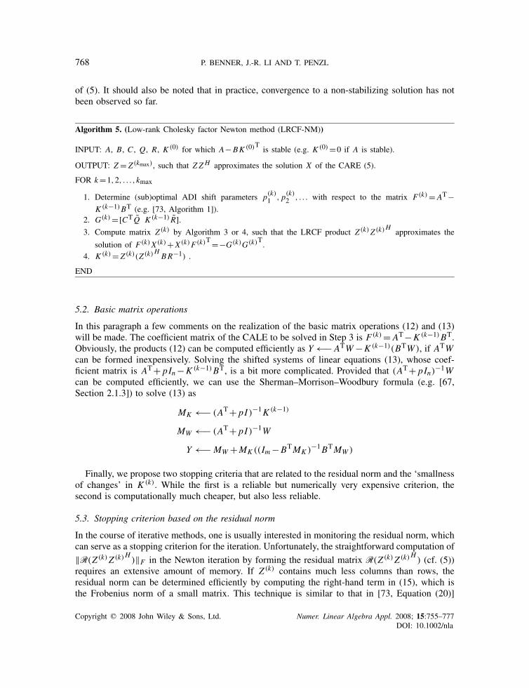
of (5). It should also be noted that in practice, convergence to a non-stabilizing solution has notbeen observed so far.

Algorithm 5. (Low-rank Cholesky factor Newton method (LRCF-NM))

INPUT: A, B, C , Q, R, K (0) for which A−BK (0)T is stable (e.g. K (0)=0 if A is stable).

OUTPUT: Z= Z (kmax), such that Z ZH approximates the solution X of the CARE (5).

FOR k=1,2, . . . ,kmax

1. Determine (sub)optimal ADI shift parameters p(k)1 , p(k)

2 , . . . with respect to the matrix F(k)= AT−K (k−1)BT (e.g. [73, Algorithm 1]).

2. G(k)=[CT Q K (k−1) R].3. Compute matrix Z (k) by Algorithm 3 or 4, such that the LRCF product Z (k)Z (k)H approximates the

solution of F(k)X (k)+X (k)F(k)T=−G(k)G(k)T.4. K (k)= Z (k)(Z (k)H BR−1) .

END

5.2. Basic matrix operations

In this paragraph a few comments on the realization of the basic matrix operations (12) and (13)will be made. The coefficient matrix of the CALE to be solved in Step 3 is F (k)= AT−K (k−1)BT.Obviously, the products (12) can be computed efficiently as Y←− ATW−K (k−1)(BTW ), if ATWcan be formed inexpensively. Solving the shifted systems of linear equations (13), whose coef-ficient matrix is AT+ pIn−K (k−1)BT, is a bit more complicated. Provided that (AT+ pIn)−1Wcan be computed efficiently, we can use the Sherman–Morrison–Woodbury formula (e.g. [67,Section 2.1.3]) to solve (13) as

MK ←− (AT+ pI )−1K (k−1)

MW ←− (AT+ pI )−1W

Y ←− MW+MK ((Im−BTMK )−1BTMW )

Finally, we propose two stopping criteria that are related to the residual norm and the ‘smallnessof changes’ in K (k). While the first is a reliable but numerically very expensive criterion, thesecond is computationally much cheaper, but also less reliable.

5.3. Stopping criterion based on the residual norm

In the course of iterative methods, one is usually interested in monitoring the residual norm, whichcan serve as a stopping criterion for the iteration. Unfortunately, the straightforward computation of

‖R(Z (k)Z (k)H )‖F in the Newton iteration by forming the residual matrix R(Z (k)Z (k)H ) (cf. (5))requires an extensive amount of memory. If Z (k) contains much less columns than rows, theresidual norm can be determined efficiently by computing the right-hand term in (15), which isthe Frobenius norm of a small matrix. This technique is similar to that in [73, Equation (20)]



and yields

‖R(Z (k)Z (k)H )‖F =

∥∥∥∥∥∥∥∥∥[CT Q ATZ (k) Z (k)]

⎡⎢⎢⎣Ih 0 0

0 0 Izk

0 Izk −Z (k)H BR−1BTZ (k)

⎤⎥⎥⎦

⎡⎢⎢⎢⎣

QTC

Z (k)H A

Z (k)H

⎤⎥⎥⎥⎦

∥∥∥∥∥∥∥∥∥F

=

∥∥∥∥∥∥∥∥R(k)

⎡⎢⎢⎣Ih 0 0

0 0 Izk

0 Izk −Z (k)H BR−1BTZ (k)

⎤⎥⎥⎦ R(k)T

∥∥∥∥∥∥∥∥F

(15)

Here, Ih, Izk denote identity matrices of proper dimensions, where zk is the number of columns ofZ (k). The triangular matrix R(k) is computed by an ‘economy size’ QR factorization U (k)R(k)=[CT Q ATZ (k) Z (k)]. Note that U (k) is not accumulated as it is not needed in the evaluation of(15). This way of evaluating the residual norm is much cheaper than computing the explicit residualmatrix, but it can still be much more expensive than computing Z (k) itself.

5.4. Stopping criterion based on K (k)

If the LQR problem is to be solved, one is interested in the state-feedback matrix K rather thanthe LRCF Z . Therefore, it seems to be reasonable to stop the iteration as soon as the changes inthe matrices K (k) become small or more precisely,

‖K (k)−K (k−1)‖F‖K (k)‖F �� (16)

Here, � is a tiny, positive constant (e.g. �=n�mach). Apparently, this criterion is very inexpensive,because K ∈Rn,m and m�n.

6. THE IMPLICIT LOW-RANK CHOLESKY FACTOR NEWTON METHOD

The solution of the LQR problem (1) and (2) is described by the optimal state-feedback matrix K ,whereas the solution of the CARE or its low-rank approximations only play the role of auxiliaryquantities. This provides the motivation for the LRCF-NM-I, which is a mathematically equivalent,implicit version of LRCF-NM. It computes an approximation to K without forming LRCF-NMiterates Z (k) and LRCF-ADI iterates Z (k)

i at all.The basic idea behind LRCF-NM-I is to generate the matrix K (k) itself in Step 3 of Algorithm 5

instead of solving the CALE for Z (k) and computing the product K (k)= Z (k)Z (k)H BR−1 inStep 4. Note that the matrix K (k) can be accumulated in the course of the ‘inner’ LRCF-ADIiteration as

K (k)= limi→∞K (k)

i



where

K (k)i := Z (k)

i Z (k)i

HBR−1=

i∑j=1

V (k)j (V (k)

j

HBR−1) (17)

Eventually, the desired matrix K is the limit of the matrices K (k)i for k, i→∞. This consideration

motivates Algorithm 6, which is best understood as a version of LRNM with an inner loop (Steps 4and 5), consisting of interlaced sequences based on Step 3 in Algorithm 3 and the partial sums givenby the right-hand term in (17). An analogous algorithm based on the real version of LRCF-ADI(Algorithm 4) can be derived in the same way.

Algorithm 6. (Implicit low-rank Cholesky factor Newton method (LRCF-NM-I))

INPUT: A, B, C , Q, R, K (0) for which A−BK (0)T is stable (e.g. K (0)=0, if A is stable).

OUTPUT: K (kmax), which approximates K given by (4).

FOR k=1,2, . . . ,kmax

1. Determine (sub-)optimal ADI shift parameters p(k)1 , p(k)

2 , . . . with respect to the matrix

F(k)= AT−K (k−1)BT (e.g. [73, Algorithm 1]).2. G(k)=[CT Q K (k−1) R].3. V (k)

1 =√−2Re p(k)

1 (F(k)+ p(k)1 In)−1G(k).

FOR i=2,3, . . . , i (k)max

4. V (k)i =

√Re p(k)

i /Re p(k)i−1(V

(k)i−1−(p(k)

i + p(k)i−1)(F(k)+ p(k)

i In)−1V (k)i−1).

5. K (k)i =K (k)

i−1+V (k)i (V (k)

iHBR−1).

END

6. K (k)=K (k)

i (k)max.

END

Most remarks on numerical aspects of LRCF-NM made in Section 5 also apply to LRCF-NM-I.Here, we only point out the differences between both methods.

It is easy to see that the computational costs of Algorithms 5 and 6 are identical. However,the memory demand of the latter is smaller. In fact, it is as low as O(n) in many situations. Forexample, this is the case when A is a band matrix with bandwidth O(1), where the shifted systemsof linear equations (13) are solved directly. Another such scenario is sparse matrices with O(n)

non-zero entries, where these systems of linear equations are solved by a Lanczos- or Arnoldi-based Krylov subspace method combined with a preconditioner, whose memory demand is O(n).In such cases, an improvement by one order of magnitude compared with standard methods isachieved. Note further that, unlike LRCF-NM, the application of LRCF-NM-I can still make sensewhen no accurate low-rank approximations to the CALE solutions exist at all.



The essential drawback of LRCF-NM-I is that the safe stopping criterion (15) cannot be applied,because Z (k) is not stored. That means one has to rely on criterion (16). Likewise, (14) must beused as stopping criterion in the inner loop, since computing the CALE residual would requireforming the iterates Z (k)

i .Basically, the same concept of a Newton–Kleinman-based ‘feedback iteration’ is used for the

numerical solution of the LQR problem in [17], although the method suggested there differs fromLRCF-NM-I in the way it is implemented. The formulation of Newton’s method in [17] is basedon the difference of two consecutive Newton steps from Algorithm 2. With the notation employedhere, this leads to

(AT−K (k−1)BT)N (k−1)+N (k−1)(A−BK (k−1)T)=N (k−2)BR−1BTN (k−2)T, k=2, . . . (18)

where X (k)= X (k−1)+N (k−1). The advantage of this formulation is that the constant term CTQCdisappears starting with the 2nd Newton step—in the first step, X (1) has to be computed as inAlgorithm 2 or needs to be known—so that the right-hand side of the Lyapunov equation has alower rank than the Lyapunov equation in (9). Unfortunately, numerical experience shows that thisiteration is less robust with respect to the accuracy of the computed solutions of the Lyapunovequations. Often, the limiting accuracy of this version of the Newton iteration is inferior to theaccuracy obtained by Algorithm 2. Also note that in [17], (18) is only used for deriving an iterationdirectly defined for the feedback matrices similar to (17), while the computation of approximatelow-rank solutions to CALEs or CAREs, which are of interest in many other applications besidesthe LQR problem, is not discussed there at all.

7. NUMERICAL EXPERIMENTS

In this section we report the results of numerical experiments with LRCF-NM and LRCF-NM-Iapplied to two large-scale test examples. These experiments were conducted at the Department ofMathematics and Statistics of the University of Calgary. The computations were performed usingMATLAB 5.3 on a SUN Ultra 450 workstation with IEEE double precision arithmetics (machineepsilon �mach=2−52≈2.2 ·10−16). In our tests, ADI shift parameters are computed by the heuristicalgorithm proposed in [73, Algorithm 1].

The following test example is used to show the performance of LRCF-NM. That means, ourgoal is to compute a LRCF Z= Z (kmax), such that Z ZH approximates the solution of (5).

Example 1Here, the dynamical system (1) arises from the model of a cooling process, which is part of theproduction of steel rails; see [82, 85]. The cooling process is described by an instationary two-dimensional heat equation, which is semidiscretized by the finite element method. The problemdimensions are n=3113,m=6, and q=6. The matrix A has the structure A=−U−1M NU−TM , whereN is the stiffness matrix and UM is the Cholesky factor of the mass matrix M . The factorizationof M and the solution of shifted systems of linear equations are realized by sparse direct methods.We consider the following three choices of R and Q:

Example 1a: R= I6, Q= I6,Example 1b: R=10−2 I6, Q= I6,Example 1c: R=10−4 I6, Q= I6.



Table I. Test results for LRCF-NM applied to Example 1.

Example 1a 1b 1c

CARE Iterations steps 5 8 12No. of columns of Z 540 492 522r(Z) 7.3×10−14 4.2×10−14 1.0×10−14

CALEs Iterations steps Minimum 45 40 42Average 45.2 41.4 44.6Maximum 46 45 46

In the three test runs, we use the inexpensive stopping criteria (16) for the Newton iteration and(14) for the LRCF-ADI iterations. We require that the latter is fulfilled in 10 consecutive iterationsteps, so that the risk of a premature termination of these inner iterations is tiny. To verify theresults of LRCF-ADI, we subsequently compute the normalized residual norm

r(Z) := ‖CTQC+ATZ ZH+Z ZH A−Z ZH BR−1BTZ ZH‖F

‖CTQC‖F (19)

using (15). Table I shows the test results. Besides r(Z), we also display the number of Newtonsteps (i.e. kmax) and the number of columns of the LRCF Z . We also provide information aboutthe number of iteration steps in the inner LRCF-ADI iterations.

Obviously, the number of Newton steps strongly depends on the choice of R. However, thenumber of columns in the delivered LRCFs Z is about the same in each test run. Note thatthis quantity is much smaller than the system order n, although the LRCF products Z ZH arevery accurate approximations to the CARE solution X in terms of r(Z). It should be noted thatsolving the CARE in this example with standard solvers like the CARE solvers in MATLAB andits toolboxes are impossible using current desktop computers.‡‡

We now investigate LRCF-NM-I using a second, more theoretical test example of scalable size.

Example 2In this example, the system (1) is related to a three-dimensional convection–diffusion problem

��

r =��r−1000�1 ��1

r−100�2 ��2

r−10�3 ��3

r+b(�)u(�)

y(�)=∫

�c(�)r d�

where �=(0,1)3, �=[�1 �2 �3]T, r=r(�,�), and r=0 for �∈��, i.e. R satisfies homogeneousDirichlet boundary conditions. b and c are the characteristic functions of the two smaller cubes(.7, .9)3 and (.1, .3)3, respectively, contained in the unit cube �. The finite-dimensional model(1) of order n=n30 is gained from a finite difference semidiscretization of the problem. Here, n0is the number of inner grid points in each space dimension. We consider three discretizations

‡‡With nowadays 64-Bit MATLAB, this has become feasible, but it still requires a much higher execution time dueto the cubic order of complexity of these solvers.



Table II. Test results for LRCF-NM-I applied to Example 2.

Example 2a 2b 2c

(n,m,q) (1000,1,1) (5832,1,1) (27000,1,1)CARE Iterations 4 4 3

eK 1.3×10−8 8.8×10−8 —CALEs Iiterations steps Minimum 103 143 96

Average 109.5 143 96Maximum 129 143 96

of different mesh size:

Example 2a: n0=10, n=1000,Example 2b: n0=18, n=5832,Example 2c: n0=30, n=27000.

The resulting matrices A are sparse and have a relatively large bandwidth. We use QMR with ILUpreconditioning to solve the shifted systems of linear equations (13). In this example, we chooseR=10−8 and Q=108.§§We solve the LQR problem (2) subject to (1) for Example 2 by computing an approximation

K (I ) to K in (4) via LRCF-NM-I. Again, we use the stopping criteria (16) and (14). To verifythe results, we also apply the (explicit) LRCF-NM with stopping criteria based on residual norms,determine the corresponding feedback K (E), and compare the results by evaluating the normalizeddeviation

eK := ‖K (I )−K (E)‖Fmax{‖K (I )‖F ,‖K (E)‖F }

This is only done for Example 2a and b, because Example 2c is too large for an application ofLRCF-NM. The results of the three test runs with LRCF-NM-I are shown in Table II.

Note that the underlying PDE has a quite strong convection term, which results in the dominanceof the skew-symmetric part of the stiffness matrix A, if a rather coarse grid is used in thediscretization. Such a dominance has usually a negative effect on the convergence of iterativemethods. In this sense, the algebraic properties of A are better for larger values of n0, whichexplains why in the third test run smaller numbers of Newton and LRCF-ADI steps are needed.

8. CONCLUSIONS

In this paper we have presented algorithms for the solution of large-scale Lyapunov equations,Riccati equations, and related linear-quadratic optimal control problems. Basically, the papercontains three contributions. First, the LRCF-ADI iteration for the computation of approximatesolutions to Lyapunov equations is described. This method had been proposed before, but inthis paper we discuss numerical aspects, which arise in context with this method, in detail. In

§§Extreme values for Q, R had to be chosen as otherwise, the convergence of Newton’s method (1–2 steps) is toofast to show any effects.



particular, we have presented a novel modification of LRCF-ADI that delivers real LRCFs andavoids complex computation. Second, we have proposed an efficient variant of Newton’s methodfor Riccati equations, which we call LRCF-NM. The third contribution is an implicit variant ofLRCF-NM, which we refer to as LRCF-NM-I. LRCF-ADI has been used as a basis for thesetwo variants of Newton’s method. LRCF-NM delivers low-rank approximations to the solutionof the Riccati equations. It can be applied to problems that are so large that the dense solutionmatrix cannot be stored in the computer memory. LRCF-NM-I can be applied to problems ofeven higher dimension, because this method directly forms approximations to the optimal statefeedback, which describes the solution of the linear-quadratic optimal control problem, rather thancomputing approximations to the solution of the corresponding Riccati equation. Note that LRCF-NM can be combined with any other solver yielding low-rank approximate solutions of Lyapunovequations, but LRCF-NM-I makes explicit use of LRCF-ADI so that the latter cannot be replacedeasily in LRCF-NM-I by other Lyapunov solvers, like, e.g. Krylov subspace methods. The resultsof numerical experiments show the efficiency of LRCF-NM and LRCF-NM-I.

REFERENCES

1. Penzl T. Lyapack users guide. Technical Report SFB393/00-33, Sonderforschungsbereich 393 NumerischeSimulation auf massiv parallelen Rechnern, TU Chemnitz, FRG 2000. Available from: http//www.tu-chemnitz.de/sfb393/sfb00pr.html.

2. Abou-Kandil H, Freiling G, Ionescu V, Jank G. Matrix Riccati Equations in Control and Systems Theory.Birkhauser: Basel, Switzerland, 2003.

3. Datta B. Numerical Methods for Linear Control Systems. Elsevier Academic Press: San Diego, CA, U.S.A.,London, U.K., 2004.

4. Mehrmann V. The Autonomous Linear Quadratic Control Problem, Theory and Numerical Solution. LectureNotes in Control and Information Sciences, vol. 163. Springer: Berlin, Heidelberg, 1991.

5. Petkov P, Christov N, Konstantinov M. Computational Methods for Linear Control Systems. Prentice-Hall:Hertfordshire, U.K., 1991.

6. Sima V. Algorithms for Linear-Quadratic Optimization, Pure and Applied Mathematics, vol. 200. Marcel Dekker,Inc.: New York, NY, 1996.

7. Banks H, Kunisch K. The linear regulator problem for parabolic systems. SIAM Journal on Control andOptimization 1984; 22:684–698.

8. Ito K. Finite-dimensional compensators for infinite-dimensional systems via Galerkin-type approximation. SIAMJournal on Control and Optimization 1990; 28:1251–1269.

9. Lasiecka I, Triggiani R. Differential and Algebraic Riccati Equations with Application to Boundary/Point ControlProblems: Continuous Theory and Approximation Theory. Lecture Notes in Control and Information Sciences,vol. 164. Springer: Berlin, 1991.

10. Morris K. Design of finite-dimensional controllers for infinite-dimensional systems by approximation. Journal ofMathematical Systems, Estimation, and Control 1994; 4:1–30.

11. Freund R. Reduced-order modeling techniques based on Krylov subspaces and their use in circuit simulation. InApplied and Computational Control, Signals, and Circuits, Datta B (ed.). vol. 1, Chapter 9. Birkhauser: Boston,MA, 1999; 435–498.

12. Freund R. Krylov-subspace methods for reduced-order modeling in circuit simulation. Journal of Computationaland Applied Mathematics 2000; 123(1–2):395–421.

13. Gawronski M. Balanced Control of Flexible Structures. Lecture Notes in Control and Information Sciences,vol. 211. Springer: Berlin, London, U.K., 1996.

14. Papadopoulos P, Laub A, Ianculescu G, Ly J, Kenney C, Pandey P. Optimal control study for the space stationsolar dynamic power module. Proceedings of the Conference on Decision and Control CDC-1991, Brighton,1991; 2224–2229.

15. Anderson B, Moore J. Optimal Control–Linear Quadratic Methods. Prentice-Hall: Englewood Cliffs, NJ, 1990.16. Lancaster P, Rodman L. The Algebraic Riccati Equation. Oxford University Press: Oxford, 1995.



17. Banks H, Ito K. A numerical algorithm for optimal feedback gains in high dimensional linear quadratic regulatorproblems. SIAM Journal on Control and Optimization 1991; 29(3):499–515.

18. Kalman R. Contributions to the theory of optimal control. Boletin Sociedad Matematica Mexicana 1960; 5:102–119.

19. Pinch E. Optimal Control and the Calculus of Variations. Oxford University Press: Oxford, U.K., 1993.20. Durrazi C. Numerical solution of discrete quadratic optimal control problems by Hestenes’ method. Supplemento

ai Rendiconti del Circolo Matematico di Palermo, Series II 1999; 58:133–154.21. Saberi A, Sannuti P, Chen B. H2 Optimal Control. Prentice-Hall: Hertfordshire, U.K., 1995.22. Green M. Balanced stochastic realization. Linear Algebra and its Applications 1988; 98:211–247.23. Varga A. On computing high accuracy solutions of a class of Riccati equations. Control-Theory and Advanced

Technology 1995; 10(4):2005–2016.24. Doyle J, Glover K, Khargonekar P, Francis B. State–space solutions to standard H2 and H∞ control problems.

IEEE Transactions on Automatic Control 1989; 34:831–847.25. Green M, Limebeer D. Linear Robust Control. Prentice-Hall: Englewood Cliffs, NJ, 1995.26. Zhou K, Doyle J, Glover K. Robust and Optimal Control. Prentice-Hall: Upper Saddle River, NJ, 1996.27. Laub A. A Schur method for solving algebraic Riccati equations. IEEE Transactions on Automatic Control 1979;

AC-24:913–921.28. Byers R. Solving the algebraic Riccati equation with the matrix sign function. Linear Algebra and its Applications

1987; 85:267–279.29. Gardiner J, Laub A. A generalization of the matrix-sign-function solution for algebraic Riccati equations.

International Journal of Control 1986; 44:823–832.30. Roberts J. Linear model reduction and solution of the algebraic Riccati equation by use of the sign function.

International Journal of Control 1980; 32:677–687. (Reprint of Technical Report No. TR-13, CUED/B-Control,Cambridge University, Engineering Department, 1971.)

31. Ammar G, Benner P, Mehrmann V. A multishift algorithm for the numerical solution of algebraic Riccatiequations. Electronic Transactions on Numerical Analysis 1993; 1:33–48.

32. Bunse-Gerstner A, Mehrmann V. A symplectic QR-like algorithm for the solution of the real algebraic Riccatiequation. IEEE Transactions on Automatic Control 1986; AC-31:1104–1113.

33. Byers R. A Hamiltonian QR-algorithm. SIAM Journal on Scientific and Statistical Computing 1986; 7:212–229.34. Benner P. Computational methods for linear-quadratic optimization. Supplemento ai Rendiconti del Circolo

Matematico di Palermo, Series II 1999; 58:21–56.35. Benner P, Faßbender H. An implicitly restarted symplectic Lanczos method for the Hamiltonian eigenvalue

problem. Linear Algebra and its Applications 1997; 263:75–111.36. Ferng W, Lin WW, Wang CS. The shift-inverted J -Lanczos algorithm for the numerical solutions of large sparse

algebraic Riccati equations. Computers and Mathematics with Applications 1997; 33(10):23–40.37. Hodel A, Poolla K. Heuristic approaches to the solution of very large sparse Lyapunov and algebraic Riccati

equations. Proceedings of the 27th IEEE Conference on Decision and Control, Austin, TX, 1988; 2217–2222.38. Jaimoukha I, Kasenally E. Krylov subspace methods for solving large Lyapunov equations. SIAM Journal on

Numerical Analysis 1994; 31:227–251.39. Benner P, Byers R. An exact line search method for solving generalized continuous-time algebraic Riccati

equations. IEEE Transactions on Automatic Control 1998; 43(1):101–107.40. Blackburn T. Solution of the algebraic matrix Riccati equation via Newton-Raphson iteration. AIAA Journal

1968; 6:951–953. See also: Proceedings of the Joint Automatic Control Conference, University of Michigan,Ann Arbor, 1968.

41. Kleinman D. On an iterative technique for Riccati equation computations. IEEE Transactions on AutomaticControl 1968; AC-13:114–115.

42. Pandey P. Quasi-Newton methods for solving algebraic Riccati equations. Proceedings of the American ControlConference, Chicago, IL, 1992; 654–658.

43. Rosen I, Wang C. A multi-level technique for the approximate solution of operator Lyapunov and algebraicRiccati equations. SIAM Journal on Numerical Analysis 1995; 32(2):514–541.

44. Zecevic A, Siljak D. Solution of Lyapunov and Riccati equations in a multiprocessor environment. NonlinearAnalysis, Theory, Methods and Applications 1997; 30(5):2815–2825.

45. Hammarling S. Newton’s method for solving the algebraic Riccati equation. NPL Report DITC 12/82, NationalPhysical Laboratory, Teddington, Middlesex, U.K., 1982.

46. Hammarling S. Numerical solution of the stable, non-negative definite Lyapunov equation. IMA Journal onNumerical Analysis 1982; 2:303–323.



47. Gajic Z, Qureshi M. Lyapunov Matrix Equation in System Stability and Control. Mathematics in Science andEngineering. Academic Press: San Diego, CA, 1995.

48. Mullis C, Roberts R. Synthesis of minimum roundoff noise fixed point digital filters. IEEE Transactions onCircuits and Systems 1976; CAS-23(9):551–562.

49. Moore B. Principal component analysis in linear systems: controllability, observability, and model reduction.IEEE Transactions on Automatic Control 1981; AC-26:17–32.

50. Glover K. All optimal Hankel-norm approximations of linear multivariable systems and their L∞ norms.International Journal on Control 1984; 39:1115–1193.

51. Lancaster P. Explicit solutions of linear matrix equation. SIAM Review 1970; 12:544–566.52. Lancaster P, Tismenetsky M. The Theory of Matrices (2nd edn). Academic Press: Orlando, 1985.53. Bartels R, Stewart G. Solution of the matrix equation AX+XB=C : Algorithm 432. Communications of the

ACM 1972; 15:820–826.54. Smith R. Matrix equation X A+BX=C . SIAM Journal on Applied Mathematics 1968; 16(1):198–201.55. Baur U, Benner P. Factorized solution of Lyapunov equations based on hierarchical matrix arithmetic. Computing

2006; 78(3):211–234.56. Grasedyck L, Hackbusch W, Khoromskij B. Solution of large scale algebraic matrix Riccati equations by use of

hierarchical matrices. Computing 2003; 70:121–165.57. Benner P, Quintana-Ortı E. Solving stable generalized Lyapunov equations with the matrix sign function. Numerical

Algorithms 1999; 20(1):75–100.58. Gardiner J, Laub A. Parallel algorithms for algebraic Riccati equations. International Journal on Control 1991;

54(6):1317–1333.59. Peaceman D, Rachford H. The numerical solution of elliptic and parabolic differential equations. Journal of the

Society for Industrial and Applied Mathematics 1955; 3:28–41.60. Wachspress E. Iterative solution of the Lyapunov matrix equation. Applied Mathematics Letters 1988; 107:87–90.61. Antoulas A, Sorensen D, Zhou Y. On the decay rate of Hankel singular values and related issues. Systems and

Control Letters 2002; 46(5):323–342.62. Grasedyck L. Existence of a low rank or H -matrix approximant to the solution of a Sylvester equation. Numerical

Linear Algebra with Applications 2004; 11:371–389.63. Penzl T. Eigenvalue decay bounds for solutions of Lyapunov equations: the symmetric case. Systems and Control

Letters 2000; 40:139–144.64. Hodel A, Tenison B, Poolla K. Numerical solution of the Lyapunov equation by approximate power iteration.

Linear Algebra and its Applications 1996; 236:205–230.65. Hu D, Reichel L. Krylov-subspace methods for the Sylvester equation. Linear Algebra and its Applications 1992;

172:283–313.66. Saad Y. Numerical solution of large Lyapunov equation. In Signal Processing, Scattering, Operator Theory and

Numerical Methods, Kaashoek MA, van Schuppen JH, Ran ACM (eds). Birkhauser: Basel, 1990; 503–511.67. Golub G, Van Loan C. Matrix Computations (3rd edn). Johns Hopkins University Press: Baltimore, 1996.68. Gudmundsson T, Laub A. Approximate solution of large sparse Lyapunov equations. IEEE Transactions on

Automatic Control 1994; 39:1110–1114.69. Ellner NS, Wachspress EL. Alternating direction implicit iteration for systems with complex spectra. SIAM

Journal on Numerical Analysis 1991; 28(3):859–870.70. Starke G. Rationale Minimierungsprobleme in der komplexen Ebene im Zusammenhang mit der Bestimmmung

optimaler ADI-Parameter. Dissertation, Fakultat fur Mathematik, Universitat Karlsruhe, Germany, 1993 (inGerman).

71. Wachspress E. The ADI model problem 1995. Available from the author.72. Li JR, Wang F, White J. An efficient Lyapunov equation-based approach for generating reduced-order models of

interconnect. Proceedings of the 36th IEEE/ACM Design Automation Conference, New Orleans, LA, 1999.73. Penzl T. A cyclic low rank Smith method for large sparse Lyapunov equations. SIAM Journal on Scientific

Computing 2000; 21(4):1401–1418.74. Li JR, White J. Low rank solution of Lyapunov equations. SIAM Journal on Matrix Analysis and Applications

2002; 24(1):260–280.75. Davis P. Circulant Matrices. Wiley: New York, NY, 1979.76. Duff I, Erisman A, Reid J. Direct Methods for Sparse Matrices. Clarendon Press: Oxford, U.K., 1989.77. Cuthill E. Several strategies for reducing the bandwidth of matrices. In Sparse Matrices and their Applications,

Rose D, Willoughby R (eds). Plenum Press: New York, NY, 1972.



78. Saak J. Effiziente numerische Losung eines Optimalsteuerungsproblems fur die Abkuhlung von Stahlprofilen.Diplomarbeit, Fachbereich 3/Mathematik und Informatik, Universitat Bremen, Bremen, September 2003.

79. Hackbusch W. Multigrid Methods and Applications. Springer: Berlin, Heidelberg, FRG, 1985.80. Stuben K. Algebraic multigrid (AMG): an introduction with applications. In Multigrid, Trottenberg U, Osterlee C,

Schuller A (eds). Academic Press: New York, 1999.81. Calvetti D, Reichel L. Application of ADI iterative methods to the restoration of noisy images. SIAM Journal

on Matrix Analysis and Applications 1996; 17:165–186.82. Penzl T. Algorithms for model reduction of large dynamical systems. Linear Algebra with Applications 2006;

415(2–3):322–343. (Reprint of Technical Report SFB393/99-40, TU Chemnitz, 1999.)83. Hochbruck M, Starke G. Preconditioned Krylov subspace methods for Lyapunov matrix equations. SIAM Journal

on Matrix Analysis and Applications 1995; 16(1):156–171.84. Simoncini V. A new iterative method for solving large-scale Lyapunov matrix equations. SIAM Journal on

Scientific Computing 2007; 29:1268–1288.85. Troltzsch F, Unger A. Fast solution of optimal control problems in the selective cooling of steel. Zeitschrift fur

Angewandte Mathematik und Mechanik 2001; 81:447–456.


Heads Up - Deloitte

Documents

Transcript of Heads Up - Deloitte