Hazardous Materials Response and Assessment DivisionOffice of Ocean Resources Conservation and AssessmentNational Ocean ServiceNational Oceanic and Atmospheric AdministrationU.S. Department of CommerceSilver Spring, Maryland

NOTICE

This report has been reviewed by the National Ocean Service of the National Oceanic and AtmosphericAdministration (NOAA) and approved for publication. Such approval does not signify that the contents of thisreport necessarily represent the official position of NOAA or of the Government of the United States, nor doesmention of trade names or commercial products constitute endorsement or recommendations for their use.

Office of Ocean Resources Conservation and AssessmentNational Ocean Service

National Oceanic and Atmospheric AdministrationU.S. Department of Commerce

The Office of Ocean Resources Conservation and Assessment (ORCA) provides decisionmakerscomprehensive, scientific information on characteristics of the oceans, coastal areas, and estuaries of theUnited States of America. The information ranges from strategic, national assessments of coastal and estuarineenvironmental quality to real-time information for navigation or hazardous materials spill response. Through itsNational Status and Trends (NS&T) Program, ORCA uses uniform techniques to monitor toxic chemicalcontamination of bottom-feeding fish, mussels and oysters, and sediments at about 300 locations throughoutthe United States. A related NS&T Program of directed research examines the relationships betweencontaminant exposure and indicators of biological responses in fish and shellfish.

Through the Hazardous Materials Response and Assessment Division (HAZMAT) Scientific SupportCoordination program, ORCA provides critical scientific support to the U.S. Coast Guard for planning andresponding to spills of oil or hazardous materials into marine or estuarine environments. Technical guidanceincludes spill trajectory predictions, chemical hazard analyses, and assessments of the sensitivity of marine andestuarine environments to spills. To fulfill the responsibilities of the Secretary of Commerce as a trustee forliving marine resources, HAZMAT's Coastal Resource Coordination program provides technical support to theU.S. Environmental Protection Agency during all phases of the remedial process to protect the environment andrestore natural resources at hundreds of waste sites each year. As another part of its marine trusteeshipresponsibilities, ORCA conducts comprehensive assessments of damages to coastal and marine resourcesfrom discharges of oil and hazardous materials.

ORCA collects, synthesizes, and distributes information on the use of the coastal and oceanic resources of theUnited States to identify compatibilities and conflicts and to determine research needs and priorities. It conductscomprehensive, strategic assessments of multiple resource uses in coastal, estuarine, and oceanic areas fordecisionmaking by NOAA, other Federal agencies, state agencies, Congress, industry, and public interestgroups. It publishes a series of thematic data atlases on major regions of the U.S. Exclusive Economic Zoneand on selected characteristics of major U.S. estuaries.

ORCA implements NOAA responsibilities under Title 11 of the Marine Protection, Research, and SanctuariesAct of 1972; Section 6 of the National Ocean Pollution Planning Act of 1978; the Oil Pollution Act of 1990; theNational Coastal Monitoring Act of 1992; and other Federal laws. It has four major line organizations: CoastalMonitoring and Bioeffects Assessment Division, Hazardous Materials Response and Assessment Division,Strategic Environmental Assessment Division, and the Damage Assessment Center.

i

CONTENTS

Page

Introduction . . . . . . . . . . . . . . . . . . . . . . . . . . . . . . . . . . . . . . . . . . . . . . . . . . . . . . . . . . . . . . 1

Site History . . . . . . . . . . . . . . . . . . . . . . . . . . . . . . . . . . . . . . . . . . . . . . . . . . . . . . . . . . 1

Previous Investigations of the Sudbury River . . . . . . . . . . . . . . . . . . . . . . . . . . . . . . . 1

NOAA's Involvement - This Study . . . . . . . . . . . . . . . . . . . . . . . . . . . . . . . . . . . . . . . . 7

Use of Bivalves in Monitoring Programs . . . . . . . . . . . . . . . . . . . . . . . . . . . . . . . . . . . . . . . . 8

Objectives . . . . . . . . . . . . . . . . . . . . . . . . . . . . . . . . . . . . . . . . . . . . . . . . . . . . . . . . . . . . . . . 11

Methods . . . . . . . . . . . . . . . . . . . . . . . . . . . . . . . . . . . . . . . . . . . . . . . . . . . . . . . . . . . . . . . . 11

Description of Study Area . . . . . . . . . . . . . . . . . . . . . . . . . . . . . . . . . . . . . . . . . . . . . 11

Mussel Collection, Processing, Deployment, and Retrieval Procedures . . . . . . . . . . 12

Mid-Test Measurements . . . . . . . . . . . . . . . . . . . . . . . . . . . . . . . . . . . . . . . . . . . . . . . 14

End-of-Test Measurements . . . . . . . . . . . . . . . . . . . . . . . . . . . . . . . . . . . . . . . . . . . . . 17

Chemical Analyses . . . . . . . . . . . . . . . . . . . . . . . . . . . . . . . . . . . . . . . . . . . . . . . . . . . . . . . . 17

Temperature . . . . . . . . . . . . . . . . . . . . . . . . . . . . . . . . . . . . . . . . . . . . . . . . . . . . . . . . . . . . . 18

Testing for Differences in Mean Temperature . . . . . . . . . . . . . . . . . . . . . . . . . . . . . 19

Testing for Differences in Temperature Range . . . . . . . . . . . . . . . . . . . . . . . . . . . . . 20

Statistical Analyses of Growth Parameters . . . . . . . . . . . . . . . . . . . . . . . . . . . . . . . . . . . . . 24

Results . . . . . . . . . . . . . . . . . . . . . . . . . . . . . . . . . . . . . . . . . . . . . . . . . . . . . . . . . . . . . . . . . . 25

Sediment Chemistry and Conventional Analyses . . . . . . . . . . . . . . . . . . . . . . . . . . . 28

Tissue Chemistry . . . . . . . . . . . . . . . . . . . . . . . . . . . . . . . . . . . . . . . . . . . . . . . . . . . . 29

Initial Tissue Mercury . . . . . . . . . . . . . . . . . . . . . . . . . . . . . . . . . . . . . . . . . . . 30

Mid-Test Tissue Mercury . . . . . . . . . . . . . . . . . . . . . . . . . . . . . . . . . . . . . . . . . 30

End-of-Test Tissue Mercury . . . . . . . . . . . . . . . . . . . . . . . . . . . . . . . . . . . . . . . 34

ii

CONTENTS, cont.

Page

RESULTS, cont.

Mussel Growth . . . . . . . . . . . . . . . . . . . . . . . . . . . . . . . . . . . . . . . . . . . . . . . . . . . . . . 35

Mid-test Observations . . . . . . . . . . . . . . . . . . . . . . . . . . . . . . . . . . . . . . . . . . . . 36

End-of-test Growth . . . . . . . . . . . . . . . . . . . . . . . . . . . . . . . . . . . . . . . . . . . . . . 36

Comparisons Between Tissue Mercury Concentrations and Growth . . . . . . . . . . . . 38

Ancillary Observations . . . . . . . . . . . . . . . . . . . . . . . . . . . . . . . . . . . . . . . . . . . . . . . . 38

Discussion . . . . . . . . . . . . . . . . . . . . . . . . . . . . . . . . . . . . . . . . . . . . . . . . . . . . . . . . . . . . . . . 39

Extent of Mercury Bioaccumulation . . . . . . . . . . . . . . . . . . . . . . . . . . . . . . . . . . . . . 39

Sources of Bioavailable Mercury . . . . . . . . . . . . . . . . . . . . . . . . . . . . . . . . . . . . . . . . . 47

Effects of Mercury Exposure . . . . . . . . . . . . . . . . . . . . . . . . . . . . . . . . . . . . . . . . . . . . . . . . 50

Effects of Temperature . . . . . . . . . . . . . . . . . . . . . . . . . . . . . . . . . . . . . . . . . . . . . . . . . . . . . 53

Reference Station and Collection Site Concerns . . . . . . . . . . . . . . . . . . . . . . . . . . . . . . . . . 55

Limits of Data Interpretation and Future Work . . . . . . . . . . . . . . . . . . . . . . . . . . . . . . . . . 55

Summary and Conclusions . . . . . . . . . . . . . . . . . . . . . . . . . . . . . . . . . . . . . . . . . . . . . . . . . 56

References . . . . . . . . . . . . . . . . . . . . . . . . . . . . . . . . . . . . . . . . . . . . . . . . . . . . . . . . . . . . . . . 58

iii

FIGURES

Page

1A The Nyanza site and the Sudbury River drainage basin in Middlesex County,Massachusetts . . . . . . . . . . . . . . . . . . . . . . . . . . . . . . . . . . . . . . . . . . . . . . . . . . . . . . . . 2

1B White Hall Reservoir Impoundment Reference (Station # 1) and Wood StreetRiver Reference (Station #2) . . . . . . . . . . . . . . . . . . . . . . . . . . . . . . . . . . . . . . . . . . . . . 3

IC Sediments collected from Reservoir 2, the first major depositional areadownstream of the Nyanza site, contained the highest concentrations of mercuryat 55 mg/kg . . . . . . . . . . . . . . . . . . . . . . . . . . . . . . . . . . . . . . . . . . . . . . . . . . . . . . . . . 4

ID Saxonville Dam (Station #5) . . . . . . . . . . . . . . . . . . . . . . . . . . . . . . . . . . . . . . . . . . . . 5

1E Sherman Street Bridge (Station #6), Fairhaven Bay (Station #7), and ThoreauStreet Bridge (Station #8) . . . . . . . . . . . . . . . . . . . . . . . . . . . . . . . . . . . . . . . . . . . . . . 6

2A Mussel rack arrangement used in study: five mussels per mesh bags, seven bagsper rack . . . . . . . . . . . . . . . . . . . . . . . . . . . . . . . . . . . . . . . . . . . . . . . . . . . . . . . . . . . 15

2B Individual mesh bags showing procedure used to distribute animals. All bags ofa common number were filled before any of the next number . . . . . . . . . . . . . . . . 15

3 Elliptio complanata showing the length, height, and width measurements madeat the beginning and end of the test . . . . . . . . . . . . . . . . . . . . . . . . . . . . . . . . . . . . . 16

4 Average daily temperature . . . . . . . . . . . . . . . . . . . . . . . . . . . . . . . . . . . . . . . . . . . . . 21

5 Boxplots showing the center and spread of the distribution of weeklytemperature ranges (C) by station. The line within the box is the median value;the height of the box is equal to the interquartile difference, or IQD (thedifference between the 3rd quartile and the 1st quartile of the data); the"whiskers" extend to the minimum/ maximum values, or a distance 15xIQDfrom the center, whichever is less. Extreme values falling outside the whiskersare indicated by horizontal lines . . . . . . . . . . . . . . . . . . . . . . . . . . . . . . . . . . . . . . . . 23

6 Initial and end-of-test tissue concentrations of total-, inorganic- andmethylmercury (ng/g-dry station (± 2 standard errors [SE]). Station 6 data arepresented for comparative purposes only open bar); they were not included inthe statistical analyses * = end-of-test concentration significantly different thaninitial concentration . . . . . . . . . . . . . . . . . . . . . . . . . . . . . . . . . . . . . . . . . . . . . . . . . 32

7 Iitial and end-of-test tissue content of total-, inorganic-, and methylmercury(ng/g-dry) by station. Station 6 data are presented for comparative purposesonly (o en bar); they were not included in the statistical analyses * = end-of-testconcentration significantly different than initial concentration . . . . . . . . . . . . . . . . 33

iv

FIGURES, cont.Page

8 Mussel growth rates (based on whole-animal wet weights), changes in tissueweight, changes in whole-animal length, and changes in shell weight by station. Station 6 data are presented for comparative purposes only (open bar); theywere not included in the statistical analyses. *** = stations that form astatistically similar group (based on non-parametric ANOVA, and multiplerange tests . . . . . . . . . . . . . . . . . . . . . . . . . . . . . . . . . . . . . . . . . . . . . . . . . . . . . . . . . . 40

9 Percent water (± 2 SE measured) in mussel tissues by station at the end of the test 41

10 Percent water vs growth rate Stations with similar mussel growth metrics are grouped 42

11 Regression relationships for mussel tissue concentrations of total, methyl-, andinorganic mercury and mussel growth rates based on changes in whole-animalwet weights. Station 6 (S6) was excluded from these regressions . . . . . . . . . . . . . . 44

12 Regression relationships for mussel tissue concentrations of total-, methyl-, andinorganic mercury and changes in mussel tissue dry weight. Station 6 (S6) wasexcluded from these regressions . . . . . . . . . . . . . . . . . . . . . . . . . . . . . . . . . . . . . . . . 45

13 Regression relationships for mussel tissue concentrations of total, methyl-, andinorganic mercury and overall increases in mussel shell length. Station 6 (S6)was excluded from these regressions . . . . . . . . . . . . . . . . . . . . . . . . . . . . . . . . . . . . . . . . . . . . . . . . . . . . . . . . . 46

14 Relationship between mussel growth rates and temperature in the SudburyRiver . . . . . . . . . . . . . . . . . . . . . . . . . . . . . . . . . . . . . . . . . . . . . . . . . . . . . . . . . . . . . . . 54

v

TABLES

Page

1 Sediment sampling and mussel deployment locations Stations were eitherimpoundment (I) or river (R) conditions. Approximate distance from suspectedmercury source is provided . . . . . . . . . . . . . . . . . . . . . . . . . . . . . . . . . . . . . . . . . . . . 12

2 Mean shell length width, height, mm), whole-animal wet weight (g), and tissueweight (g-wet) measurements (± standard deviation) by station for animals at T0(n= 10 5) . . . . . . . . . . . . . . . . . . . . . . . . . . . . . . . . . . . . . . . . . . . . . . . . . . . . . . . . . . . 13

3 Summary of temperature conditions by station during study period . . . . . . . . . . . 19

4 Results of Newman-Keuls Multiple Range Test on weekly temperature ranges . . . . . . . . . . . . . . . . . . . . . . . . . . . . . . . . . . . . . . . . . . . . . . . . . . . . . . . . . . . . . 22

5A Mussel measurement at the start of the test (initial) and after 42 days' (mid-test) exposure in the Sudbury River. Mussels in bags I and 2 were used . . . . . . . . . . . . . . . . . . . . . . . . . . . . . . . . . . . . . . . . . . . . . . . . . . . . . . . . . . . . . . . 26

5B Mussel measurement after 84 days exposure (end of test) in the Sudbury River.Mussels in bags 3 through 7 were used . . . . . . . . . . . . . . . . . . . . . . . . . . . . . . . . . . . 27

6 Results of selected trace element analyses and conventional parametersfor sediments collected from Whitehall Reservoir and the Sudbury River . . . . . . . . 29

7 Tissue mercury concentrations (±SD) in mussels collected from LakeMassesecum at the start of the test, growth, and tissue mercuryconcentrations by station for mussels after 84 days exposure in theSudbury River . . . . . . . . . . . . . . . . . . . . . . . . . . . . . . . . . . . . . . . . . . . . . . . . . . . . . . 31

8 Results of correlation analyses (r values) on selected parameters. Boldnumbers = significant correlation (rcrit=0.707; 95% confidence level) . . . . . . . . . . . 37

9 Ranges in response for the different growth metrics measured at the endof the study . . . . . . . . . . . . . . . . . . . . . . . . . . . . . . . . . . . . . . . . . . . . . . . . . . . . . . . . 38

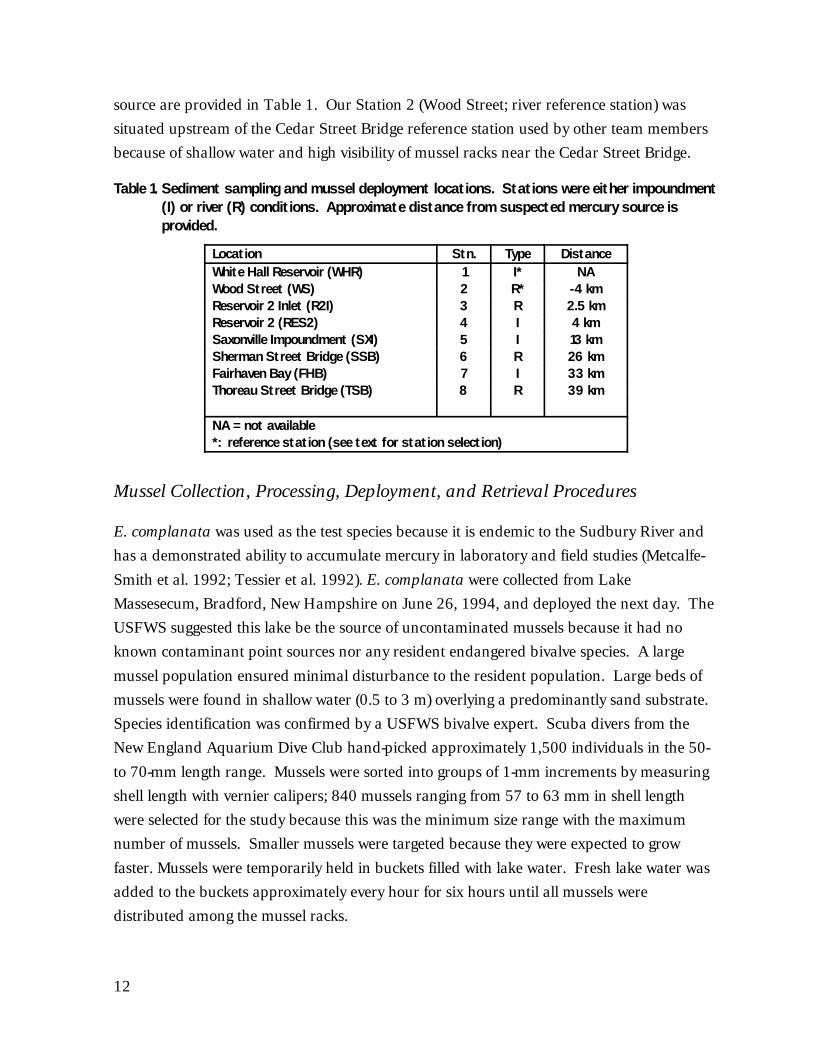
10 Significant correlation coefficients . . . . . . . . . . . . . . . . . . . . . . . . . . . . . . . . . . . . . . 39

vi

ACKNOWLEDGMENTS

The authors would like to thank the following people for their participation in this effort:

Susan von Oettingen of the U.S. Fish and Wildlife Service for her support and guidance in

locating a source of test animals and assistance during the initial collection and setup; Tom

Gloria and the New England Dive Club for their excellent job of collecting mussels from and

returning unused individuals to Lake Massesecum, and measuring animals during the setup;

Pat Boyd for her technical expertise, perseverance, and good humor during all phases of the

project; Doug Smith for technical expertise regarding freshwater mussels; David Strayer for

guidance regarding mussel population ecology; and the EVS staff (Berit Bergquist, Dan

Hennessy, Rich Sturim, and Kimberly Galimanis) who provided support during field and

report preparation activities. A special thanks to the Lake Massesecum campground for

access to the lake and space during the initial setup activities.

1

Introduction

Site History

The Nyanza Chemical Waste Dump Site (Nyanza) is the former location of several textile dyeproduction companies near the Sudbury River in Ashland, Massachusetts (MA; Figure 1A),approximately 35 km west of Boston. Mercury and chromium were used as catalysts in theproduction of textile dyes from 1917 to 1978. Approximately 2.3 metric tons of mercurywere used per year from 1940 to 1970 [JBF Scientific Corporation (JBF) 1972] withapproximately 45 to 57 metric tons of mercury released to the Sudbury River during thisperiod (JBF 1973). From 1970 until the facility closed in 1978, wastes were treated on siteand wastewater was discharged to Ashland’s town sewer system. These changes in wastemanagement practices reduced the amounts of mercury released to the Sudbury River tobetween 23 and 30 kg per year. Since dye production stopped in 1978, the property hasbeen leased to various light industries and commercial companies. The Nyanza site wasadded to the National Priorities List and declared a Superfund site in 1982.

Land along the Sudbury River ranges from semi-rural to urban-suburban. There are severalimpoundments, including Mill Pond and the Saxonville Dam Impoundment, behind intactor partially collapsed dams built for milling operations during the early 1900s (NOAA 1993). Below the Saxonville Dam, the river is primarily depositional and meanders through anextensive floodplain. Figures 1B through 1E detail the pathway of the Sudbury River fromits inception near Cedar Swamp to its confluence with the Assabet River to form theConcord River. These figures also illustrate the various dams and bays associated with theSudbury River.

Previous Investigations of the Sudbury River

Numerous studies have been conducted since 1970 to assess mercury contamination in the

Sudbury River (JBF 1971, 1972, 1973; MA Division of Fish and Wildlife (DFW) 1977; MA

Department of Environmental Quality Engineering (DEQE) 1980, 1986; Maietta 1990; U.S.

Fish and Wildlife Service (USFWS) 1990; NUS 1992). The most intensive and thorough

sampling was conducted as part of the remedial investigation for Operable Unit III (the

Sudbury River and wetlands next to the site) in 1989 and 1990 (c.f., NUS 1992). The

Operable Unit III sampling plan emphasized depositional areas of the Sudbury River, such

as those near stream confluences or inside river bends. Sediments collected from Reservoir

2 (Figure 1C), the first major depositional area downstream of the Nyanza site, contained the

7

highest concentrations of mercury at 55 mg/kg; sediments collected near the Concord River

had mercury concentrations as high as 0.5 mg/kg. This latter concentration was

approximately five times higher than observed in background sediments collected from

Southville Pond, Sudbury Reservoir, and Reservoir 3, where mercury concentrations were all

less than the detection limit of 0.1 mg/kg. Two background samples collected in the

downstream section of Reach 1 had sediment mercury concentrations of 1.6 and 0.5 mg/kg

(Figure 1A). These historical data suggest that mercury contamination extends throughout

the Sudbury River.

Fish collected from the major reservoirs on the Sudbury River contained tissue

concentrations of mercury as high as 12 mg/kg (MA DEQE 1980). Limited data are

available regarding mercury in fish between 1971 and 1990. When the fish tissue data from

1971 (JBF 1972) are compared to 1990 data (NUS 1992) on a qualitative basis, it does not

appear that there has been a substantial reduction in bioavailable mercury. In 1971, fish

tissues contained approximately 10 mg/kg; in 1990, concentrations were detected as high as

8 mg/kg. Mercury was detected in 74 percent of the fish sampled between the site and

Concord, Massachusetts 39 km away; a maximum concentration of 7.6 mg/kg was

measured in fish collected from Reservoir 2 (NUS 1992). In Fairhaven Bay, approximately

33 km downstream of the Nyanza site, 93 percent of the fish sampled contained detectable

concentrations of mercury with a maximum concentration of 3.2 mg/kg.

Since mercury appeared to be readily bioavailable within the Sudbury River system, the

Massachusetts Department of Environmental Protection (MA DEP) and the U.S.

Environmental Protection Agency (EPA) posted and maintained signs advising against

consumption of fish from the river. Studies have been performed in the Sudbury River to

evaluate mercury bioavailability and the geographical extent of the mercury contamination

in biota. General trends have been established for the predominant form of mercury within

sediments and the biological effects of exposure to mercury. However, additional data are

necessary to specify the sources of mercury in sediments and biota, and to conclude whether

environmental concentrations pose a substantial threat to aquatic resources.

NOAA’s Involvement - This Study

To address these concerns and develop a scientifically defensible ecological risk assessment

for the Sudbury River (Operable Unit-IV), EPA has elicited the help of other Federal agencies

who have interests and concerns regarding natural resources and the improvement of

impacted habitats. This study is one part of a larger, multi-agency program. Decisions about

the site will be based on the combined results from all of the studies. The findings presented

8

in this report could be enhanced when supporting data are available.

Because habitats could be used for migration, spawning, and nursery activities, the lower

reaches of the Sudbury River are of concern to NOAA, who acts for the U.S. Department of

Commerce as a trustee for natural resources. Trust resources (e.g., anadromous fish) will

have access to the Sudbury River as far upstream as the Saxonville Dam Impoundment

(approximately 13.5 km from the Nyanza site) when proposed fish passage facilities on the

Concord River become operational. Sections of the river above this dam provide habitat for

the catadromous American eel. As part of EPA’s joint effort, NOAA conducted a study to

measure total- and methylmercury bioaccumulation and to estimate chronic effects on a

resident bioindicator species. The freshwater mussel Elliptio complanata was selected to

test effects from exposure to mercury-contaminated water, sediments, and food. Mussels

were transplanted both to selected sites along the Sudbury River and a reference site in a

distant reservoir. Our goal was to estimate mercury exposure and effects that could be used

in EPA’s quantitative ecological risk assessment. The information obtained in the mussel

transplant study will also help NOAA assess potential impacts to trustee natural resources.

Use of Bivalves in Monitoring Programs

Resident and transplanted populations of both freshwater and marine bivalves have been

used as biomonitors of environmental contamination for almost 30 years, although the use

of marine bivalves like Mytilus spp. has been more extensive (Bedford et al. 1968; Godsil

and Johnson 1968; Young et al. 1976; Eganhouse and Young 1978b; Phillips 1980;

McMahon 1991). Monitoring resident bivalve populations for the accumulation of

contaminants has been the most common form of biomonitoring, but the development of

transplant methodologies has increased the use of caged animals and has facilitated synoptic

measurements of bioaccumulation and bioeffects (Salazar and Salazar 1995). This in-situ

approach combines the experimental control of laboratory studies with the environmental

realism of field monitoring to assess site-specific contamination and effects. Freshwater and

marine mussels are probably the most common bioindicators because they are ubiquitous,

sedentary, and responsive to their environment on both micro- and macro-geographical

scales (Green et al. 1985). Their hard shells make them easy to collect, handle, cage, and

measure; their sedentary nature makes them excellent for transplant studies. Mussels can

integrate and accumulate bioavailable contaminants at concentrations orders of magnitude

above those found in other environmental media (e.g., water or sediment). Their soft tissues

can be analyzed to estimate contaminant uptake and exposure. Even though they can

9

tolerate elevated contaminant concentrations, mussels respond to environmental perturba-

tions by altering their physiology and metabolism. Growth is commonly used as a measure

of effects because it provides an integration of many biological processes (Salazar and

Salazar 1995).

E. complanata is a filter-feeding bivalve that is widely distributed in the streams of

northeastern North America (Magnin and Stanczykowska 1971; Curry 1977; Heit et al.

1980). It is a long-lived, sedentary organism that comes into contact with both sediment and

water during filtration activities (feeding and respiration), and it can accumulate trace metals,

including mercury, and organic contaminants (Kauss and Hamdy 1991; Metcalfe-Smith et

al. 1992). E. complanata has been used in a number of monitoring studies with both

resident populations (Tessier et al. 1984; Creese et al. 1986; Hinch and Stephenson 1987;

Servos et al. 1987; Russell and Gobas 1989; Metcalfe and Charlton 1990; Campbell and

Evans 1991; Elder and Collins 1991; Metcalfe-Smith and Green 1992; Metcalfe-Smith et al.

1992) and transplanted animals (Curry 1977; Hinch and Green 1989; Day et al. 1990;

Koenig and Metcalfe 1990; Kauss and Hamdy 1991; Langdon 1993). Freshwater bivalves

are increasingly used as sentinels for trace metals, including mercury. The database

associating bioaccumulation, bioeffects, and contamination in various environmental

compartments such as water and sediment is making the results more useful in

environmental assessments.

Bioaccumulation of contaminants by the freshwater mussel E. complanata has been used to

evaluate several major waterways, including the Niagara, St. Clair, and St. Mary’s rivers

(Creese et al. 1986). In 1977, Curry (1977) proposed caged E. complanata as a practical

approach for detecting organic trace contaminants in water after an exposure period of four

to six weeks. Creese et al. (1986) presented a preliminary, standard, biomonitoring

methodology for caged E. complanata based on their ability to accumulate environmental

contaminants such as organochlorine compounds and heavy metals. Hinch and Green

(1989) studied the effects of source and destination on growth and metal uptake in E.

complanata reciprocally transplanted in Ontario lakes. Kauss and Hamdy (1991) used

caged E. complanata to assess the availability of polynuclear aromatic hydrocarbons in

sediment. Metcalfe-Smith et al. (1992) used two species of freshwater mussels (E.

complanata and Lampsilis radiata) to evaluate the relationships between concentrations of

metals in sediment and in mussel tissues. Metcalfe-Smith et al. (1992) also sought to

determine whether mussels could provide useful information on the bioavailability of

sediment-bound metals that is necessary to predict environmental effects. Metcalfe-Smith

(1994) found that Elliptio complanata demonstrated a broader response range to metal

10

exposures (including mercury) than other species, suggesting that this species may be more

sensitive to changes in pollution status.

Tessier et al. (1992) evaluated mercury bioaccumulation kinetics in E. complanata and

suggested that this species concentrates mercury primarily from the water column (e.g., in

the dissolved phase or as food particles). Others have found similar results with different

bivalve species (Davies and Pirie 1978; Fowler et al. 1978; King and Davies 1987;

Muncaster et al. 1990).

Investigators have shown that mercury is biologically available in marine, estuarine, and

freshwater systems with availability partially dependent on the form of mercury present

(Fowler et al. 1978; Riisgård and Hansen 1990). Mercury undergoes methylation and

behaves differently than other “metals.” Methylmercury, the form of particular concern,

more closely resembles organic compounds than metals with respect to mobility,

bioavailability, accumulation/depuration, and toxicity. Previous studies have shown a

preferential accumulation of methylmercury over other forms of mercury (Fowler et al. 1978;

Tessier et al. 1984; Mohlenberg and Riisgrd 1990; Metcalfe-Smith et al. 1992).

Relationships between the concentrations of mercury in water and in tissues have been

demonstrated more consistently than those for sediment and tissue (Fowler et al. 1978;

Tessier et al. 1994; Malley et al. in press). Although the concentrations of mercury measured

in the water column are usually much lower than in bivalve tissues, the relationship between

sediment and tissue mercury concentrations is equivocal, because sediment concentrations

have been shown to be higher, lower, or the same as tissue concentrations (Bryan and

Langston 1992; Metcalfe-Smith et al. 1992). Similarly, a number of studies have shown

positive correlations between tissue burdens and sediment concentrations (Langston 1982

1986; Bryan and Langston 1992) while others have shown no relationship (Luoma 1977;

Rubinstein et al. 1983; Lasorsa and Allen-Gil 1995).

11

Objectives

The primary objectives of the mussel transplant study conducted by NOAA were to:

! Demonstrate the extent of bioavailable mercury within the downstream reaches of the

Sudbury River resulting from operations at the Nyanza site;

! Identify areas that could act as sources of mercury for transport downstream; and

! Determine the effect of mercury exposure on a resident species.

The data generated in this study can be used to identify areas that show significant mercury

bioaccumulation and biological impacts as candidates for EPA remedial action.

Methods

Description of Study Area

Mussels (E. complanata) were transplanted to eight stations during this study: six stations in

the river downstream of the Nyanza site, one reference station upstream (river reference) of

the facility, and one reference station in White Hall Reservoir (reservoir reference; Figures

1A-1E). The White Hall Reservoir is connected to the Sudbury River by a small creek. EPA

and other agencies participating in the investigation (NOAA, the National Biological Survey,

the U.S. Geological Survey (USGS), the USFWS, and the Army Corps of Engineers) selected

these reference stations and the impoundment stations. Each team member attempted to

establish stations in the areas identified in the investigation.

We selected stations that represented a gradient of mercury contamination associated with

sediments. Highest sediment mercury concentrations were expected at Station 3,

approximately 2.5 km from the Nyanza site. Stations were located as far downstream as the

Concord River, approximately 39 km from the site. Final station locations were situated

near the shore (water depths 0.6 to 1.3 m) for easy access from the shoreline.

To compare mercury availability in free-flowing and impounded areas in the river, three

stations plus one reference were located in impoundments (Stations 1, 4, 5, and 7) and three

stations plus one reference were located in free-running segments of the Sudbury River

(Stations 2, 3, 6, and 8). Stations 6 and 8 were located within wetland areas of the river in

an attempt to assess availability of mercury where methylmercury production may be higher

(St. Louis et al. 1994). Station descriptions and distances from the suspected mercury

12

source are provided in Table 1. Our Station 2 (Wood Street; river reference station) was

situated upstream of the Cedar Street Bridge reference station used by other team members

because of shallow water and high visibility of mussel racks near the Cedar Street Bridge.

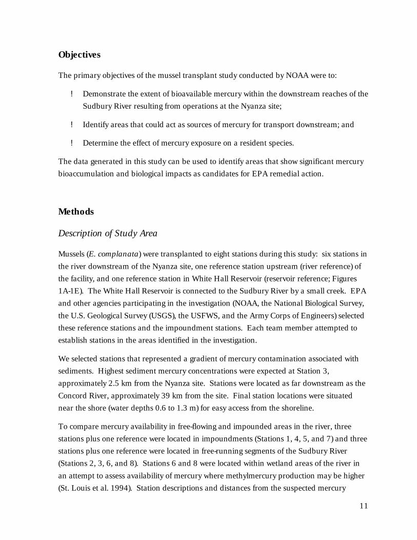
Table 1. Sediment sampling and mussel deployment locations. Stations were either impoundment(I) or river (R) conditions. Approximate distance from suspected mercury source isprovided.

Location Stn. Type DistanceWhite Hall Reservoir (WHR) 1 I* NAWood Street (WS) 2 R* -4 kmReservoir 2 Inlet (R2I) 3 R 2.5 kmReservoir 2 (RES2) 4 I 4 kmSaxonville Impoundment (SXI) 5 I 13 kmSherman Street Bridge (SSB) 6 R 26 kmFairhaven Bay (FHB) 7 I 33 kmThoreau Street Bridge (TSB) 8 R 39 km

NA = not available*: reference station (see text for station selection)

Mussel Collection, Processing, Deployment, and Retrieval Procedures

E. complanata was used as the test species because it is endemic to the Sudbury River and

has a demonstrated ability to accumulate mercury in laboratory and field studies (Metcalfe-

Smith et al. 1992; Tessier et al. 1992). E. complanata were collected from Lake

Massesecum, Bradford, New Hampshire on June 26, 1994, and deployed the next day. The

USFWS suggested this lake be the source of uncontaminated mussels because it had no

known contaminant point sources nor any resident endangered bivalve species. A large

mussel population ensured minimal disturbance to the resident population. Large beds of

mussels were found in shallow water (0.5 to 3 m) overlying a predominantly sand substrate.

Species identification was confirmed by a USFWS bivalve expert. Scuba divers from the

New England Aquarium Dive Club hand-picked approximately 1,500 individuals in the 50-

to 70-mm length range. Mussels were sorted into groups of 1-mm increments by measuring

shell length with vernier calipers; 840 mussels ranging from 57 to 63 mm in shell length

were selected for the study because this was the minimum size range with the maximum

number of mussels. Smaller mussels were targeted because they were expected to grow

faster. Mussels were temporarily held in buckets filled with lake water. Fresh lake water was

added to the buckets approximately every hour for six hours until all mussels were

distributed among the mussel racks.

13

Each rack consisted of a square frame (made from three-quarter-inch plastic PVC pipe) to

which seven mesh bags were attached, each containing five mussels (total 35 mussels per

rack; Figure 2A). Tube-shaped, plastic mesh bags (four-inch diameter; 0.5-inch mesh size)

were knotted at each end to prevent mussels from escaping. Mussels within the bags were

separated from each other by constricting the mesh with plastic washers. A random-number

table was used to distribute the 24 racks among the eight stations (three racks per station). A

total of 105 mussels was deployed at each of the eight stations. Procedures described by

Salazar and Salazar (1995) were used to ensure a statistically similar mussel size distribution

among all racks. The mesh bags on each rack were numbered from 1 to 7. Starting with the

smallest-sized class mussels, all bags of a given number were filled consecutively (e.g., all 24

racks had #1 bags filled before #2 bags). All mussels in each 1-mm size class were

distributed before the next size class was used (Figure 2B).

Before placement in mesh bags, each mussel was measured for shell length, width, height

(Figure 3), and whole-animal wet weight. Each shell measurement was made to the nearest

0.1 mm with vernier calipers; whole-animal wet weights were made to the nearest 0.01 g with

a portable analytical balance. Mean values (± standard deviation [SD]) by rack and station

measured at the start of the test are provided in Table 2. The field assessment procedures of

Salazar and Salazar (1995) are based on shell length and whole-animal wet weight; the

additional shell measurements were made in this study to provide background information

on this species of freshwater mussels. At the start of the test, there were no statistical

differences in mussel lengths or whole-animal wet weights among the individual racks, or the

groups of three racks randomly selected for each station (" = 0.05).

Table 2. Mean shell (length, width, height; mm), whole-animal wet weight (g), and tissue weight (g-wet)measurements (± SD) by station for animals at T0 ( n = 105).

Station Length1 Width1 Height1Whole-Animal Wet

WeightTissue Weight2

1-WHR 59.5 (1.55) 15.2 (1.21) 30.7 (1.64) 15.15 (2.56) 3.87 (0.54)2-WS 59.5 (1.69) 15.1 (1.14) 30.6 (1.61) 15.18 (2.38) 3.88 (0.51)3-R2I 59.5 (1.50) 15.4 (2.24) 30.7 (1.33) 15.10 (2.00) 3.86 (0.42)4-RES2 59.5 (1.45) 15.0 (1.11) 30.4 (1.45) 15.07 (2.23) 3.85 (0.47)5-SXI 59.5 (1.55) 15.3 (1.22) 30.8 (1.30) 15.09 (2.15) 3.86 (0.46)6-SSB 59.6 (1.43) 15.2 (1.11) 31.3 (3.37) 15.23 (2.17) 3.89 (0.46)7-FHB 59.6 (1.40) 15.2 (1.17) 30.5 (1.35) 15.12 (2.03) 3.87 (0.43)8-TSB 59.6 (1.42) 15.1 (1.13) 31.0 (1.47) 15.11 (2.23) 3.87 (0.47)1 See Figure 3 for measurement information.

2 Tissue weights calculated from regression equation based on a subsample of 30 individuals; see text for further details.

14

Mussels prepared for field-deployment were held in racks overnight in Lake Massesecum.

Racks were retrieved the next morning and mesh bags containing mussels were placed in

coolers containing only ice and newspaper. (Newspaper was used to separate mussels from

the ice.) The mussels were not held in water during transportation. Mussels were moved

from New Hampshire to Massachusetts by automobile. Deployment started at Station 8 and

finished at Station 1. Mussels were out of water from 3 to 12 hours. Based on the current

literature and discussions with Dr. Stansbery (Curator of Bivalve Mollusks, College of

Biological Sciences, Ohio State University), this is the preferred method to transport E.

complanata as it results in minimal stress for periods of up to 72 hours.

Before deployment at each station, mussel bags were removed from the cooler and attached

to the PVC racks with an overhand knot and plastic cable ties. Each of three racks was

tethered with a one-meter line to a cinder block and placed on the river bottom. All practical

attempts were made to situate the caged mussels over soft (i.e., muddy) substrates; areas with

large rocks or boulders were avoided.

Three sediment grabs were collected from each station for chemical analysis using a hand-

held ponar. The grab was checked for integrity and completeness after sediment collection.

Samples that contained rocks or other foreign material were discarded as were samples in

grabs that did not completely close upon retrieval. On shore, the grab was released and

sediments were deposited into a plastic tray. The top 5 cm of each sample was collected for

analysis of selected chemicals and conventional parameters.

Mid-Test Measurements

Mid-test measurements were made after 42 days’ exposure (August 8, 1994) to ensure that

the mussel racks were undisturbed and not overly fouled; to determine whether the mussels

were growing; to determine whether mussels were accumulating mercury in the soft tissues;

and to obtain another datum point for rate of mercury accumulation.

Bags 1 and 2 were removed from each rack and all surviving mussels (n=10) processed.

Mussels were presumed missing (i.e., not dead) if their respective space in the bag was

empty. Mussels were considered dead only if empty shells or gaping, unresponsive

individuals were found. Mussels were held in tubs containing site water to help ensure that

the internal shell chambers were completely filled prior to whole-mussel, wet-weight

measurement. Whole-animal wet-weights, shell measurements (i.e., length, width, and

height), and tissue wet-weights were determined for each animal. For each rack, tissues from

all mussels in

16

Bags 1 and 2 (n < 10) were composited and chemically analyzed for total mercury. All

equipment used during the shucking procedure was first decontaminated with a warm soap

wash, then rinsed, acetone-rinsed, hexane-rinsed, air-dried, and wrapped in foil.

During the mid-test measurements, high mortality (>50 percent) was noted for animals

transplanted at Station 6 (Sherman Street Bridge). Dissolved oxygen concentrations were

suspected to be low at the original deployment location due to the high density of aquatic

vegetation in the immediate area and the presence of a sulfur odor. The State of

Massachusetts confirmed that episodes of low dissolved oxygen occurred during the summer

in the area of the Sherman Street Bridge (Goldman Environmental Consultants, Inc. 1994).

After retrieving Bags 1 and 2, the three racks were relocated approximately 50 m upstream

in a less vegetated area.

17

End-of-Test Measurements

The mussel racks were retrieved on September 18, 1994, after 84 days’ exposure. The mesh

tubes containing mussels were removed from the arrays and placed in coolers containing

crushed ice and newspaper; again using newspaper to separate the mussels from the ice.

Mussels were measured according to methods previously described. Decontamination

procedures were the same as at mid-test. Tissues from all surviving mussels for each rack

(for all stations except Station 6: minimum of 19; maximum of 25 mussels) were pooled and

frozen before chemical analysis. This procedure provided three replicates at all sites except

Station 6 where only two replicates were available due to high mortality. A minimum of

eight mussels were used in the composites for Station 6.

Chemical Analyses

The 24 sediment samples (three replicates for each of eight stations) collected during mussel

deployment were analyzed for selected metals (antimony, arsenic, cadmium, chromium, lead,

and mercury) and conventionals (total solids, total organic carbon, and grain size). The

metals selected for analysis were the same as those analyzed by other agencies evaluating

Sudbury River sediments. Antimony, arsenic, and lead were analyzed by graphite furnace

atomic absorption spectrophotometry (GFA), cadmium and chromium were analyzed by

inductively coupled argon plasma (ICP), and mercury by cold vapor atomic absorption (CVA).

All metals analyses and grain-size determinations were conducted according to Puget Sound

Estuary Program (PSEP) protocols (PSEP 1989). Total organic carbon (TOC) was analyzed

according to the procedure provided in Plumb (1981) and total solids according to U.S. EPA

Method 160.3 SM 2540 B (APHA/AWWA/WEF 1992).

Mussel tissues were analyzed for total mercury and methylmercury concentrations according to

the methods provided in Bloom (1989, 1992) and Bloom and Fitzgerald (1988). Initial total

and methylmercury concentrations in mussel tissues before deployment in the Sudbury River

were estimated by measuring a subsample of 30 mussels (61.3 to 63.8 mm in length; ten

mussels in each of three replicates) collected from Lake Massesecum. Mid-test mussels were

analyzed only for total mercury; end-of-test analyses included both methyl- and inorganic

mercury. Methylmercury was analyzed in 50 -Fl aliquots of potassium hydroxide digest by

aqueous-phase ethylation, isothermal gas-chromatograph separation, and cold vapor atomic

fluorescence (CVAFS) detection (instrument detection limits of approximately 0.2 picograms).

Total mercury was analyzed in 50-Fl aliquots of acid digest by SnCl2 reduction, dual gold

amalgamation, and CVAFS detection. Detection limits for total and methylmercury were

18

0.0005 and 0.0002 Fg/g, respectively. The dry fraction material of the samples was determined

by drying an aliquot (approximately 5 grams) overnight at 105EC in aluminum drying pans.

Inorganic mercury concentration was calculated as the difference between total and

methylmercury:

Inorganic mercury concentration (ng/g) = total mercury concentration (ng/g) -

methylmercury concentration (ng/g) Equation (1)

The total and methylmercury content were determined for all tissue samples by the following

equation:

Content (ng) = Concentration (ng/g) * Animal Weight (g) Equation (2)

Inorganic mercury content was calculated as the difference between total- and methylmercury:

Inorganic mercury content (ng) = total mercury content (ng) - methylmercury

content (ng) Equation (3)

The content information can be used to determine whether growing mussels have accumulated

mercury, since the overall mercury concentrations (ng/g-dry weight) may actually decrease in

fast-growing individuals due to growth dilution. Salazar and Salazar (1995) and Riisgård and

Hansen (1990) have shown that faster-growing, smaller animals take up more contaminants,

even though tissue concentrations decrease. Therefore, mercury content provides data on net

uptake or depuration and was used in this study to determine whether mussels transplanted in

the Sudbury River for 84 days contained more mercury than they did at the onset of the study.

Temperature

Water temperature conditions at each station were recorded at 24-minute intervals (i.e., 60

observations per day) from June 26, 1994 to September 16, 1994 using one in-situ

computerized data logger per station (HoboTemp, Onset Instruments). Data were downloaded

from the logging devices using the instruments’ data recovery software. Temperature data for

Station 1 (reference station) were recorded only from June 26, 1994 to July 13, 1994, due to a

19

malfunction in the temperature recording device. Data for this station was not included in the

analysis.

Water temperature conditions were fairly similar with short- and long-term cycles during the first

half of the study and declining temperatures after the first week of August. Minimum and

maximum temperatures are summarized in Table 3. Apparent differences between upstream

and downstream stations, and between river and impoundment stations were observed. These

differences were investigated using statistical approaches to test two primary hypotheses:

1. Is the mean temperature different across stations, and

2. Is the range of temperatures different across stations?

Table 3. Summary of temperature conditions by station during study period.

Station Date Range Minimum—Maximum ( C)1 6/26 - 7/13/94 22.7 - 31.52 6/26 - 9/17/94 13.2 - 26.93 6/26 - 9/17/94 14.8 - 28.14 6/26 - 9/17/94 18.1 - 29.65 6/26 - 9/17/94 16.5 - 29.46 6/26 - 9/17/94 15.1 - 29.07 6/26 - 9/17/94 15.6 - 30.08 6/26 - 9/17/94 15.6 - 30.0

The water temperatures measured during the study are within the natural range for E.

complanata in the northeastern United States (Stansbery personal communication 1994), and

are not expected to be a significant factor for either bioaccumulation or growth in this species.

However, these data were subjected to a statistical evaluation to investigate the presence of any

trends. The two hypotheses are addressed separately in the following sections.

Testing for Differences in Mean Temperature

The temperature series at Stations 2-8 displayed similar patterns with daily and seasonal cycles,

as well as both short and long-term trends. These series showed very strong autocorrelations (a

measure of the dependence between observations of the same series). The standard analysis of

mean differences (e.g., t-test) requires independent observations. Therefore, the data from these

series required transformation and subsampling to produce an uncorrelated series which would

20

adequately summarize the data.

The data sets were reduced to daily mean temperatures to reduce both the internal variability

and autocorrelation of each temperature series (Figure 4). The series of daily means for all

stations displayed very similar patterns. Each series of daily means (each of length 82) exhibited

autocorrelation beyond 20 lags. Each of the seven stations which had sufficient temperature

data was paired with every other station resulting in 21 station pairs. An independent sample of

daily mean differences of the stream temperatures was associated with each of these pairs. The

pattern of these differences indicate whether one station is consistently warmer than another; if

the differences are not distinguishable from zero, then the two stations can be said to have

similar daily mean temperatures. The test of the hypothesis for differences in mean temperature

was accomplished by comparing each independent sample of differences between two stations

to zero via a one-sample t-test (using a two-tailed -level of 0.05). The results indicate that the

mean temperatures were significantly different between most stations, with the exception of

Stations 4 and 8, Stations 5 and 6, Stations 5 and 7, and Stations 5 and 8. The order of the

mean temperatures was as follows:

Sta 2 (WS) < Sta 3 (R2I) < Sta 6 (SSB) < Sta 5 (SXI) < Sta 7 (FHB) < Sta 8 (TSB) < Sta 4 (RES2).

This temperature pattern is consistent with water residence times in a river system. Upstream

stations (shorter water residence times) are cooler than the downstream stations, and stations in

impoundments (i.e., Stations 4, 5, and 7) are generally warmer than faster flowing river stations.

Testing for Differences in Temperature Range

E. complanata is highly adaptable and can readily acclimate to changes in temperature; its

natural habitat ranges from the Great Lakes area to the Gulf of Mexico and it therefore naturally

experiences a wide temperature range (Stansbery personal communication 1994). To assess the

effects of environmental conditions on growth in E. complanata, we evaluated temperature

ranges over periods of one week. This time interval was selected because: seven days is a

manageable time period, as opposed to comparisons based on an hourly or daily basis, it is

expected to have some biological relevance, and it is a common interval used to measure

changes in environmental conditions and growth in aquatic organisms.

21

22

Although some dramatic changes in temperature were observed on a daily basis, the overall

trend was for temperatures to change slowly over time, with marked differences evident within

periods of four to seven days. From a biological viewpoint, a seven-day period should provide

time for the manisfestation and measurement of effects due to exposure to adverse condition.

Although we did not monitor the mussels on a weekly basis, we calculated growth rates as

mg/week.

We calculated 12 weekly temperature ranges per station by subtracting minimum weekly

temperatures from the maximum weekly. This series did not need additional subsampling

because it was not significantly autocorrelated. The sample distribution (Figure 5) showed

sufficient approximate normality and equality of variances to apply a one-way ANOVA.

Weekly temperature ranges among the stations were signigicantly different (p = 0.032). To

identify which stations in particular were different from one another, a Newman-Keuls Multiple

Range test was used. The results of the analysis are presented in Table 4.

Table 4. Results of Newman-Keuls Multiple Range Test on weekly temperature ranges.

Station: 4 (RES2) 7 (FHB) 8 (TSB) 5 (SXI) 3 (R2I) 6 (SSB) 2 (WS)Mean of Ranges (EEC) 3.66 4.37 4.38 4.50 4.87 4.91 5.08Stations with significant difference: Sta 4 vs Sta 2 (p = 0.025*) Sta 4 vs Sta 6 (p = 0.051*)

*Value is interpolated and not exact.

Station 4 had the lowest average range of temperatures over the weekly periods. Stations 2 and4 were the only significantly different stations in their range of weekly temperatures. The resultsof the temperature range analysis are also consistent with the physical influence of flow patternsin rivers. Longer water residence times affect both the mean temperature as well as thevariability due to an extended exposure to the heat in the surrounding environment. Residencetime effects are consistent with our study’s results. Stations located in impoundments(particularly Station 4 located in Reservoir 2), had warmer temperatures and lower variabilitythan would be expected from their relative position along the river system.

23

24

Statistical Analyses of Growth Parameters

Growth of individual mussels was measured in this study. Individuals were identified by rack

position and measured at the beginning and end of the study. Growth can be estimated from a

variety of mussel metrics. In this study, mussel growth was calculated from changes in whole-

animal wet weight, shell length, shell weight, and tissue weight. Changes in whole-animal wet

weight and length provide integrated measures of animal response. The error associated with

the whole-animal wet-weight measurement is primarily due to air within the shell cavity that

could add a low bias to the measurements. The error associated with the length measurement is

uncertainty in locating the longest axis. The researchers minimized initial variability within and

among stations by selecting mussels within a very narrow size range.

Changes in tissue weights can also be used as an estimate of mussel growth. Determining soft-

body wet-weights is a destructive process. Thus, the initial tissue weight measurement could

only be estimated from the following regression equation generated for the subsample of 30

individuals measured at the start of the test:

Initial tissue weight (g-wet) = 0.21 (whole-animal wet-weight) + 0.66 Equation (4)

The error associated with using end-of-test tissue weight as an estimate of growth is primarily

due to not knowing the exact tissue weight of the individuals before deployment.

Shell weight also provides a measure of animal growth. However, as with tissue weights, only

end-of-test shell weights can be obtained because this is a destructive process. The following

regression equation was generated from the subsample of 30 individuals measured at the start

of the test and used to estimate initial shell weights for the transplanted individuals:

Initial shell weight (g-wet) = 0.44 (whole-animal wet-weight) + 0.21 Equation (5)

All mussel metrics were recorded and analyzed; whole-animal wet weight, tissue weight, and

shell weight were the metrics with the greatest potential for identifying stressed animals. To

reduce variability attributable to water and facilitate comparisons with current literature, the dry-

weight data were used throughout our analyses. Both dry- and wet-weight tissue mercury data

are provided in this report. The wet- to dry-weight conversions were made using the percent-dry

fraction data provided by the analytical laboratory. There was a very high, significant

correlation between wet and dry tissue weights (r2=0.97, "=0.05).

25

Mussels selected for deployment were between 57 and 63 mm in length. At the start of the test,

mussels were sorted by length (to the nearest 0.1 mm), weighed (to the nearest 0.01 g), and

distributed among the mesh bags. An analysis of variance (ANOVA; n = number of arrays) was

used to ensure even distribution within arrays. No statistical difference was found in the

distribution of mussels among the racks. Following the rack-by-rack analysis, the data for all

mussels assigned to a station were pooled and re-analyzed on a station-by-station basis.

Growth rates (mg/wk) were calculated for individuals according to the following equation:

Growth rate (mg/wk) = weight(f)- weight(i)/number of weeks Equation (6)

All data sets were analyzed for homogeneity in variances (Zar 1974) before conducting ANOVAs

and Duncan’s multiple range test (NW Analytical StatPak, Ver. 4.1) to determine differences

among stations. If data did not meet the requirements for parametric analyses, the non-

parametric equivalents were used (i.e., Kruskal-Wallis non-parametric ANOVA and Dunn’s

Multiple Comparison Test). At no station was there a significant difference among the three

replicate racks. This allowed pooling of the data for each station and analyses on a station-by-

station basis. A correlation analysis was run between selected variables to help identify trends

and potential relationships. All statistical analyses were run at the 95-percent confidence level.

Results

Overall, the test was considered successful because all mussel racks were retrieved. Results for

mid- and end-of-test mussel measurements are presented in Tables 5A and B. End-of-test

survival ranged from 83 to 95 percent at all sites except Station 6, where it was 36 percent;

growth rates for these mussels were significantly lower than other downstream sites. Mussels at

Stations 7 and 8 had the greatest increases in tissue weight, shell length, and whole-animal wet

weight. Survival at Stations 1 and 2 was 83 and 91 percent, respectively; animals at these

stations had negative changes in whole-animal wet weight suggesting no growth (Table 5B).

Since mussels at Stations 1 and 2 appeared to be in poor condition and the mercury

concentrations were much higher than expected, they did not qualify as reference stations, and

the planned comparisons could not be made. These data will be included in the statistical

analyses, but the results must be interpreted with caution. Although the data for Station 6 will

be included for completeness, they were not included in statistical comparisons because of high

mortality, low growth rates, and the station relocation at mid-test.

26

Table 5A. Mussel measurements at the start of the test (initial) and after 42 days’ (mid-test) exposure inthe Sudbury River. Mussels in Bags 1 and 2 were used.

Initial T0 (n=30) Mid-test Increase % %Station Mean ±SD Mean ±SD Mean ±SD Moisture N Survival

Tissue Weights (g-wet)1-WHR 3.47 0.27 3.72 0.64 0.25 0.57 86.9 23 77%2-WS 3.58 0.40 3.49 0.58 -0.09 0.46 87.6 29 97%3-R2I 3.56 0.37 3.85 0.45 0.29 0.42 86.9 30 100%4-RES2 3.55 0.37 4.84 0.48 1.29 0.43 84.9 22 73%5-SXI 3.66 0.36 5.11 0.55 1.44 0.52 84.3 30 100%6-SSB 3.62 0.26 4.25 0.67 0.63 0.77 87.2 13 43%7-FHB 3.69 0.39 5.36 0.71 1.67 0.44 82.9 24 80%8-TSB 3.62 0.33 5.70 0.89 2.08 0.66 82.5 27 90%

Whole-Animal Length (mm)1-WHR 57.8 1.10 57.8 1.10 0.0 0.37 23 77%2-WS 57.9 0.83 57.9 0.89 -0.1 0.20 29 97%3-R2I 57.8 0.70 57.9 0.74 0.0 0.25 30 100%4-RES2 57.9 0.73 59.6 1.22 1.6 0.66 22 73%5-SXI 58.1 0.72 59.3 1.08 1.2 0.70 30 100%6-SSB 58.2 0.68 58.7 1.04 0.5 0.26 13 43%7-FHB 58.0 0.66 59.0 1.08 1.0 0.94 24 80%8-TSB 58.0 0.65 59.5 1.33 1.6 1.14 27 90%

Growth RateWhole-Animal Wet-Weight (g) (mg/wk)1

1-WHR 13.27 1.3 13.22 1.33 -0.05 0.41 -24 23 77%2-WS 13.77 1.9 13.37 1.74 -0.40 0.34 -64 29 97%3-R2I 13.68 1.7 13.68 1.69 0.00 0.30 0 30 100%4-RES2 13.64 1.7 15.38 1.75 1.74 0.74 252 22 73%5-SXI 14.16 1.7 15.69 2.03 1.53 0.78 255 30 100%6-SSB 13.95 1.2 14.72 1.31 0.77 0.35 15 13 43%7-FHB 14.28 1.8 16.14 1.98 1.86 0.96 281 24 80%8-TSB 13.93 1.6 16.04 1.98 2.11 1.21 318 27 90%

27

Table 5B. Mussel measurements at the start of the test (initial) after 84 days’ exposure (end of test) in theSudbury River. Mussels in Bags 3 through 7 were used.

Initial Exposed Increase % %Mean ±SD Mean ±SD Mean ±SD Moisture N Survival

Tissue Weights (g-wet)1-WHR 4.03 0.54 4.29 0.7 0.26 0.49 88.4 62 83%2-WS 4.00 0.50 3.99 0.6 -0.01 0.49 87.1 68 91%3-R2I 3.98 0.39 4.26 0.5 0.28 0.50 86.5 70 93%4-RES2 3.98 0.46 5.79 0.8 1.81 0.61 85.4 71 95%5-SXI 3.94 0.47 5.09 0.9 1.15 0.92 84.9 65 87%6-SSB 4.00 0.48 5.33 0.7 1.33 0.68 84.3 27 36%7-FHB 3.94 0.43 6.26 1.1 2.32 1.15 82.8 66 88%8-TSB 3.97 0.49 6.87 1.2 2.90 1.15 81.8 65 87%

Whole-Animal Length (mm)1-WHR 60.2 1.2 60.5 0.3 0.2 0.29 62 83%2-WS 60.1 1.6 60.2 0.1 0.1 0.26 68 91%3-R2I 60.2 1.1 60.4 0.2 0.3 0.27 70 93%4-RES2 60.1 1.2 62.0 1.9 1.9 1.14 71 95%5-SXI 60.3 1.1 62.1 1.8 1.9 1.65 65 87%6-SSB 60.2 1.2 60.6 0.4 0.3 0.64 27 36%7-FHB 60.2 1.0 62.4 2.2 2.1 1.35 66 88%8-TSB 60.1 1.2 62.8 2.7 2.6 1.76 65 87%

Growth RateWhole-Animal Wet-Weight (g) (mg/wk)1

1-WHR 15.90 2.56 15.62 2.43 -0.28 0.57 -21 62 83%2-WS 15.74 2.34 15.43 2.29 -0.31 0.49 -38 68 91%3-R2I 15.67 1.82 15.80 1.62 0.13 0.44 23 70 93%4-RES2 15.64 2.16 17.84 2.16 2.20 1.28 185 71 95%5-SXI 15.46 2.21 17.62 2.60 2.16 1.99 198 65 87%6-SSB 15.74 2.26 16.25 2.37 0.51 1.75 46 27 36%7-FHB 15.46 2.02 18.82 2.17 3.36 1.86 270 66 88%8-TSB 15.59 2.29 19.26 2.40 3.67 1.51 303 65 87%1Growth Rates based on changes in whole-animal wet-weight

28

Sediment Chemistry and Conventional Analyses

Mean total mercury concentrations in sediments ranged from 0.07 at Station 7 (Fairhaven Bay)

to 17.9 mg/kg-dry at Station 3 (Reservoir 2 Inlet). The second highest total mercury

concentration, 5.4 mg/kg-dry, was measured in sediments from Station 5 (Saxonville

Impoundment). Although the high measurement was over two orders of magnitude greater than

the low measurement, sediments from six of the eight stations had total mercury concentrations

less than or equal to 0.5 mg/kg (Table 6). Total-mercury concentrations in sediments collected

from Reservoir 2 (Station 4) were very low. Elevated concentrations of chromium and lead were

also detected in sediments, with the highest concentrations at Stations 3 (Reservoir 2 Inlet) and

5 (Saxonville Impoundment; Table 6).

Correlation analyses were run on the following metals measured in sediment: mercury,

chromium, lead, and cadmium. These metals were selected for correlation analysis because

measured concentrations in sediments exceeded concentrations known to produce adverse

effects in aquatic organisms in other studies; mercury and chromium are the primary

contaminants of concern associated with Nyanza. Results of the correlation analyses (Table 7)

show a strong, significant association between mercury and chromium, with a correlation

coefficient of 0.98 (r0.05,(2),6=0.707). Mercury was not strongly associated with other metals, but

there was a strong association between cadmium and lead (r2 = 0.91). Both mercury and

chromium concentrations were moderately associated with TOC concentration (r2= 0.72 and

0.77, respectively). Lead and cadmium were weakly associated with TOC (r2 = 0.53 and 0.5,

respectively).

The grain size analyses showed sediments varying in composition (Table 6). Although attempts

were made to locate stations in similar substrate types, Stations 2, 4, 7 and 8 were

predominantly sand (>80 percent sand) while the remaining stations were predominantly fines

(61 to 80 percent silt and clay). TOC concentrations ranged from 1.62 to 11.7 percent (Table

6). The correlation analysis indicates a significant positive correlation between fines and TOC

(r2 = 0.80).

29

Table 6. Results of selected trace element analyses and conventional parameters for sediments collectedfrom Whitehall Reservoir and the Sudbury River.

1-WHR 2-WS 3-R21 4-RES2 5-SXI 6-SSB 7-FHB 8-TSB

Trace Elements (mg/kg-dry) 1

Mercury 0.17 0.11 17.9 0.17 5.4 0.5 0.07 0.36Chromium 24.3 10.3 152.3 14 78 22.3 7.9 28Lead 132.7 107 225 17.7 410 58.7 5.4 40Antimony U (0.4) U (0.3) 1.4 U (0.2) 1.1 U (0.5) U (0.2) U (0.2)Arsenic 5.9 3.7 12.2 3 11.9 8.1 9.2 10.7Cadmium U (0.8) 0.6 3.3 0.4 10 3.6 0.3 1

Physical Parameters (%) 2

TOC 5.93 3.45 11.7 3.37 7.7 10 1.62 4.58Total solids

Grain size

22.87 43.97 18.57 49.43 19.28 18.98 65.98 38.79

Sand 17 82 30 80 38 34 90 85Silt 70 14 58 16 46 42 6 10Clay 10 3 10 2 14 22 4 5U Undetected; concentration in parentheses equals the detection limit.1 Concentrations were determined as the mean of three replicate samples.2 Measurements were made on one sample only at each station, except for grain size at Station 6, determined

as a mean of triplicate samples.

Detection Limits (mg/kg)Cadmium 0.2Chromium 0.5Arsenic 0.1Lead 0.1Antimony 0.1

Mercury 0.05

Tissue Chemistry

All tissue chemistry data reported here (Table 7; Figures 6 and 7) represent the mean of three

replicate samples and have been rounded to two significant digits. Although results in Table 7

are presented on both a wet- and dry-weight basis, only the dry-weight data are discussed in the

text. The laboratory that performed the chemical analyses obtained a uniform homogenate.

The laboratory conducted both duplicate analyses of the same digest, and duplicate digestions of

a mussel composite. Their results indicate that the variance between replicates is similar to the

variance associated with multiple extractions of a given sample (approximately 16 to 20 percent

variability).

30

The laboratory quality assurance results provided for tissue analyses were within the specified

control limits for this study. Analytical and injection replicate results for both total and

methylmercury analyses indicated that results are within the acceptable limits of ±35 relative

percent difference (RPD). Samples were not affected by the total- or methylmercury detected in

the method blanks, because all sample results were greater than five times the amount of

contamination found in the corresponding method blank.

Standard Reference Materials (SRM) were analyzed for both total and methylmercury

determinations on mussel tissue. All SRM percent recoveries for total mercury in the initial,

middle, and final stages of the study fell within the control limits. The SRM percent recovery for

methylmercury in the initial stage also fell within control limits. Methylmercury analysis was not

conducted for samples collected in the middle stage. The SRM percent recovery for

methylmercury in the final stage fell slightly below the control limits (86 percent vs. 92 percent).

Initial Tissue Mercury

Tissues of mussels collected from Lake Massesecum had mean total and methylmercury

concentrations of 640 (±103) and 140 (±9.29) ng/g-dry, respectively (Table 7). These

concentrations were much higher than expected for mussels collected from a relatively pristine

lake. Methylmercury accounted for approximately 22 percent of the total mercury. Initial mean

tissue total mercury content was 510 (±125) ng; initial mean tissue methylmercury content was

110 (±18.2) ng. Initial mean tissue inorganic mercury concentration was 500 ng/g-dry; initial

mean tissue inorganic mercury content was 400 ng per mussel.

Mid-Test Tissue Mercury

After 42 days’ exposure, mussels had mean tissue total mercury concentrations ranging from

330 to 930 ng/g-dry. The tissue total mercury concentrations decreased with distance from

Nyanza (Table 7; Figure 6). Mean total mercury concentrations in mussel tissues at the

reference stations (Stations 1 and 2) increased by approximately 110 to 140 ng/g-dry. Mean

total mercury concentrations in tissues of mussels closest to Nyanza (Station 3) increased by

about 290 ng/g-dry. Mean tissue total mercury concentrations decreased by 90 to 310 ng/g-dry

for mussels at all other stations.

31

Table 7. Tissue mercury concentrations (±SD) in mussels collected from Lake Massesecum at the start of the test; growth and tissue mercuryconcentrations by station for mussels after 84 days’ exposure in the Sudbury River.

StationGrowth Rate

(mg/wk)Total Hg

(ng/g wet)Methyl Hg(ng/g wet)

Total Hg(ng/g dry)

Methyl Hg(ng/g dry)

Inorganic Hg(ng/g dry)

Total HgContent (ng)

Methyl HgContent (ng)

InorganicContent (ng) % MeHg

Initial - 120 (20) 25 (1.66) 640 (103) 140 (9.29) 500 510 (125) 110 (18.2) 400 22

Mid Test1-WHR -24 99 (22.4) - 750 (165) - - 370 (116) - - -2-WS -64 96 (17.7) - 780 (179) - - 330 (66.3) - - -3-R2I 0 120 (9.60) - 930 (79.4) - - 470 (60.0) - - -4-RES2 252 84 (8.02) - 550 (47.1) - - 400 (54.3) - - -5-SXI 255 85 (7.81) - 550 (70.0) - - 440 (56.4) - - -6-SSB 15 67 (13.6) - 520 (104) - - 310 (66.5) - - -7-FHB 281 63 (8.66) - 370 (60.6) - - 330 (45.2) - - -8-TSB 318 58 (6.46) - 330 (31.9) - - 320 (50.7) - - -

End of Test1-WHR -21 100 (5.43) 41 (4.19) 890 (85.5) 360 (46.7) 530 440 (70.4) 180 (28.5) 270 402-WS -38 110 (17.3) 33 (5.41) 850 (71.9) 260 (44.3) 600 440 (90.5) 130 (28.0) 310 303-R2I 23 130 (5.53) 43 (3.89) 950 (33.3) 320 (29.6) 640 550 (73.1) 180 (25.2) 370 334-RES2 185 100 (26.3) 38 (2.08) 690 (228) 260 (24.8) 430 570 (140) 220 (33.4) 350 385-SXI 198 78 (5.40) 29 (6.47) 520 (56) 200 (49.8) 320 390 (64.5) 150 (31.0) 240 386-SSB 46 94 (26.6) 27 (3.96) 590 (127) 170 (42.8) 420 450 (108) 150 (25.5) 350 337-FHB 270 69 (8.95) 24 (2.44) 400 (51.1) 140 (11.0) 260 430 (92.5) 150 (31.2) 280 348-TSB 303 62 (5.96) 24 (0.81) 340 (35.7) 130 (3.5) 210 430 (59.5) 170 (20.1) 260 39- = Not Measured or Not Applicable

32

200

400

600

800

1000

Tota

l Hg

(ng/

g-dr

y) Initial

A: Total Mercury Concentration* * *

* *

500

Initial

B: Methyl Mercury Concentration

200

400

300

100MeH

g (n

g/g-

dry) *

* ** *

Figure 6. Initial and end-of-test tissue concentrations of total, methyl, and inorganic mercury (ng/g-dry) by station (+/- 2SE). * indicates end-of-test tissue concentration significantly different than initial concentration. Station 6 data are presented for comparative purposes only (open bar); they were not included in the statistical analyses.

Inor

gani

c H

g (n

g/g-

dry)

200

400

600

800

Sta 1WHR

Sta 2WS

Sta 3R2I

Sta 4RES2

Sta 5SXI

Sta 6SSB

Sta 7FHB

Sta 8TSB

Initial

C: Inorganic Mercury Concentration

**

33

250

MeH

g (n

g-dr

y)

200

150

100

50

* * ** * *B: Methyl Mercury Content

Initial

400

600

800

Tota

l Hg

(ng-

dry)

A: Total Mercury ContentInitial

200

C: Inorganic Mercury Content

Inor

gani

c H

g (n

g-dr

y)

Initial

100

200

300

400

500

Sta 1WHR

Sta 2WS

Sta 3R2I

Sta 4RES2

Sta 5SXI

Sta 6SSB

Sta 7FHB

Sta 8TSB

Figure 7. Initial and end-of-test tissue content of total, methyl, and inorganic mercury (ng-dry) by station (+/- 2SE). * indicates end-of-test tissue content significantly different than initial content. Station 6 data are presented for comparative purposes only (open bar); they were not included in the statistical analyses.

34

End-of-Test Tissue Mercury

The mean concentrations of total, inorganic, and methylmercury in mussel tissues decreased

downstream (with distance away) from Nyanza (Figure 6). Compared to initial values, mean

methylmercury content in mussel tissues increased at all stations, while mean inorganic content

decreased and mean total content remained about the same (Figure 7).

Mean tissue total mercury concentrations ranged from 340 ng/g-dry at Station 8 to 950 ng/g-dry

at Station 3. These concentrations were similar to mid-test tissue total mercury concentrations.

The downstream gradient of decreasing tissue total mercury concentrations persisted through

the end of the test (Figure 4). Mean tissue total mercury concentrations for mussels at the two

reference stations (Stations 1 and 2) increased above the mid-test concentrations to final

concentrations of 890 and 850 ng/g-dry, respectively. These concentrations were slightly lower

than those measured in mussels deployed at Station 3, the station closest to Nyanza. Mean

tissue total mercury concentrations were significantly higher at Stations 1, 2, and 3 at the end of

the test than at the start; mean tissue total mercury concentrations at Stations 7 and 8 were

significantly lower at the end of the test than at the start ("=0.05). At the end of the test, the

tissue total mercury concentrations for mussels at Stations 1, 2, and 3 (850 to 950 ng/g) were

significantly higher than for mussels at Stations 7 and 8 (340 to 400 ng/g).

Mean tissue methylmercury concentrations ranged from 130 ng/g-dry to 360 ng/g-dry, with the

lowest concentration measured in a mussel from Station 8 and the highest at Station 1. Tissue

methylmercury concentrations generally paralleled those of total mercury (Figure 6):

concentrations were significantly higher at Stations 1 through 4 at the end of test than at the

start, and the tissue methylmercury concentrations for mussels at Stations 1 and 3 (320 to 360

ng/g) were significantly higher than measured in mussels at Stations 7 and 8 (130 to 140 ng/g).

The mean inorganic mercury concentration in tissues decreased for mussels at all stations

downstream of Station 3 (Figure 6). Tissue concentrations of inorganic mercury for the

reference mussels and Station 3 mussels were higher than the initial concentration, but this

increase was not statistically significant. The tissue inorganic mercury concentrations at Stations

7 and 8 were significantly lower than at the start of the test.

The mean concentrations of total-, inorganic-, and methylmercury in tissues of mussels at

Stations 1 and 2 (the reference stations) were not significantly different than the concentrations

measured in mussels transplanted at the station situated nearest Nyanza. The data suggest that

35

mussels at Stations 1 and 2 were exposed to bioavailable mercury and thus may not be

appropriate as reference animals.

The mean tissue content data indicate that there were no significant changes in the total amount

of mercury within the mussel tissues (Table 7; Figure 7). Except for Stations 3 and 4, the total

mercury content in all mussel tissues was slightly lower at the end of the test. Total mercury

content increased slightly for mussels at Stations 3 and 4. Methyl-mercury content per mussel

increased at all stations during the course of the test (Table 7; Figure 7). This increase was

statistically significant for mussels at all stations except Stations 2 and 6, where the

methylmercury content increased by 20 and 30 ng, respectively. For mussels at the other

stations, the methylmercury content increased by 40 to 110 ng, with the greatest increase at

Station 4. Mussels at all stations had inorganic mercury contents that were lower than at the

start of the test, but these decreases were not statistically significant (Figure 7).

The proportion of methylmercury within the total mercury content of mussels increased at all

stations during the test. Methylmercury accounted for 30 to 40 percent of the total mercury

content in mussels at the end of the test, compared to an initial composition of 22 percent

methylmercury (Table 7).

The correlation analysis for total mercury concentrations in sediment and tissues resulted in an

r-value of 0.446 (Table 7). This relationship is not significant at the 95-percent confidence level

(r0.05,(2),6= 0.707; Zar 1974). Correlation analyses were also conducted on TOC-normalized

sediment mercury concentrations, but normalizing did not raise the correlation. Since high total

mercury concentrations were predicted for Station 4 sediments, and other investigators’ results

were up to two orders of magnitude higher, their chemistry data were used in a separate

correlation analysis. This substitution did not increase the correlation. An r-value of 0.381 was

obtained for sediment total mercury versus tissue methylmercury concentration (Table 8).

Mussel Growth

The best estimates of mussel growth in this study were final tissue weights and change in tissue

weight, change in whole-animal wet weights, and change in shell length. Although changes in

shell weight differed among stations, the ecological significance of these data are unclear (Figure

8; Table 5B). Apparent changes in shell width and height were within measurement error and

were not useful metrics. The ranges in response measured among animals at all test stations at

the end of the study are presented in Table 9.

36

Mid-test Observations

Mid-test survival rates varied from 43 to 100 percent (Table 5A). The low survival for

individuals transplanted to Station 6, in addition to observations of sulfur in the sediment and

dense plant material, caused us to relocate Station 6 mussels mid-test.

Mussels at Stations 1 and 2 decreased slightly in whole-animal wet-weight; mid-test growth rates

(based on changes in whole-animal wet weights) for these mussels were -24 and -62 mg/week,

respectively. Mussels at Station 3 (near Reservoir 2 Inlet) did not grow. Mussels appeared to

grow at all stations below Nyanza, although mussels at Station 6 had a very low growth rate (15

mg/week). Mussels from Station 8 had the highest growth rates at 318 mg/week. Table 5A

presents mid-test growth measurements.

Changes in tissue weight and shell length were similar to the changes observed for whole-animal

wet weights. There was little change for animals at Stations 1, 2, 3, and 6, while mussels at

Stations 4, 5, 7, and 8 showed increases.

End-of-test Growth

In general, mussel growth increased from Station 1 to Station 8 as shown by increases in whole-

animal wet weights, lengths, tissue weights, and shell weights (Figure 8). Based on changes in

tissue weight, whole-animal wet-weight, and whole-animal shell length, Stations 1, 2, and 3 had

very low or negative growth and form a statistical grouping. Stations 7 and 8 had the highest

growth and also form a separate statistical grouping. It is difficult to include Stations 1 and 2 in

these comparisons. Mussels at both the White Hall Reservoir and Station 2 had unexpectedly

high tissue concentrations of mercury. Beginning with Station 4, mussel growth rates generally

increased with distance away from the site, except for Station 6.

Considering all the metrics evaluated, mussels at Stations 1, 2, and 3 demonstrated little to no

growth (Figure 8; Table 5B). Based on changes in whole-animal wet-weight, mussels at Stations

7 and 8 had the highest growth rates. Similarly, statistical analyses confirm that mussel growth

metrics from Stations 1, 2, and 3 were similar (although only Stations 1 and 2 sometimes form

the group), as they were at Stations 7 and 8 (Figure 8).

Figure 9 shows the change in percent water in mussel tissues during the test period. There is a

decreasing gradient with distance from the White Hall Reservoir. End-of-test percent water

concentrations ranged from 81.8 to 88.4; initial concentration was 81.9 percent. Mussels at

Stations 7 and 8 showed very little change in water concentration during the test. There was a

37

Table 8. Results of correlation analyses (r-values) on selected parameters. Bold numbers = significantcorrelation (rcrit = 0.707; 95% confidence level)

A. Sediment Metal Concentrations and Conventionals versus tissue mercury levels.Mercury Chromium Lead Cadmium TOC % Sand % Silt % Clay

Mercury 1Chromium 0.981 1Lead 0.547 0.662 1Cadmium 0.393 0.527 0.913 1Total Organic Carbon 0.720 0.767 0.529 0.503 1% Sand -0.447 -0.525 -0.569 -0.451 -0.797 1% Silt 0.182 0.559 0.582 0.405 0.740 1% Clay 0.182 0.267 0.383 0.528 0.767 1Tissue[THg] 0.446Tissue[MeHg] 0.381Tissue-THg-Content 0.359Tissue-MeHg-Content 0.176

B. Tissue mercury levels versus mussel metrics (with Sta6 included in analyses).|------------Concentration-----------

||--------------Content---------------|

Tissue Tissue Tissue Tissue Tissue Tissue Tissue Percent[THg] [MeHg] [InoHg] THg MeHg InoHg Weight Water

Tissue Weight -0.924 -0.858 -0.910 -0.184 0.031 -0.299 1 0.965Whole Animal Growth -0.982 -0.754 -0.918 -0.232 0.149 -0.198 0.913 0.868Whole Animal Length -0.850 -0.684 -0.893 -0.249 0.207 -0.172 0.858 0.791Shell Weight -0.873 -0.746 -0.894 -0.176 0.183 -0.135 0.902 0.844

C. Tissue mercury levels versus mussel metrics (without Sta6 included in analyses).|------------Concentration-----------

||--------------Content---------------|

Tissue Tissue Tissue Tissue Tissue Tissue Tissue Percent[THg] [MeHg] [InoHg] THg MeHg InoHg Weight Water

Tissue Weight -0.925 -0.881 -0.911 -0.195 0.050 -0.309 1 0.972Whole Animal Growth -0.947 -0.875 -0.946 -0.203 0.080 -0.340 0.949 0.945Whole Animal Length -0.941 -0.853 -0.948 -0.210 0.111 -0.368 0.923 0.907Shell Weight -0.931 -0.872 -0.924 -0.144 0.013 -0.274 0.941 0.925

38

Table 9. Ranges in response for the growth metrics measured at the end of the study.

Growth Metric Lowest Value Highest Value Observed

Growth rate based on whole-animal wet weight -21 mg/wk 303 mg/wk

Change in tissue weight (g-wet) 0 g 2.90 g

Change in whole-animal shell length 0.1 mm 2.6 mm

Change in empty shell weight -0.25 g 2.01 g

negative relationship between percent water and growth rate, with the data falling into four

distinct groups (Figure 10).

Comparisons Between Tissue Mercury Concentrations and Growth.

Correlation analyses (NW Analytical StatPak, Ver. 4.1) were conducted on various mussel

growth metrics and mercury concentrations (Table 8). Station 6 was not included in these

analyses because the station was considered an outlier. The significant correlation coefficients

resulting from that analysis are shown in Table 10.

No significant correlations were found for tissue mercury content (on a per-animal basis) and

mussel growth metrics. Station 6 data were excluded from these analyses because of the high

mortality and the low growth rates observed for these mussels. Regression analyses (NW

StatPak, Ver. 4.1) were conducted on the three forms of mercury and the three mussel growth

metrics (Figures 11-13). Based on the r2 values, for each mussel growth metric, the relationship

between methylmercury is not as strong as for either total or inorganic mercury.

Ancillary Observations

Mussels and racks at reference Station 1 (White Hall Reservoir) looked clean and scrubbed.

Unlike the other stations, there was very little algal fouling or growth of plant matter directly on

the racks. Mussels deployed at Station 2 had very fragile shells and the plastic tag labels were

39

Table 10. Significant correlation coefficients.

Comparison r valueWAWW* growth vs. tissue total mercury concentration -0.95WAWW growth vs. tissue methylmercury concentration: -0.88WAWW growth vs. tissue inorganic mercury concentration -0.95EOT** tissue weight vs. tissue total mercury concentration -0.93EOT tissue weight vs. tissue methylmercury concentration -0.88EOT tissue weight vs. tissue inorganic mercury concentration -0.91EOT shell length vs. tissue total mercury concentration -0.94EOT shell length vs. tissue methylmercury concentration -0.85EOT shell length vs. tissue inorganic mercury concentration 0.95EOT shell weight vs. tissue total mercury concentration -0.93EOT shell weight vs. tissue methylmercury concentration -0.87EOT shell weight vs. tissue inorganic mercury concentration: -0.92* whole-animal wet weight** end of test (Critical r-value r0.05,(2),5=0.755; all correlations are significant at the 95-percent confidence level.)

were dissolved. Mussels deployed at Station 4 (Reservoir 2) had an oily sheen and distinct odor

of petroleum product. Mussels at Station 6 (Sherman Street Bridge) required relocation because

of presumed low-oxygen conditions and poor mussel survival. Most of the dead mussels were in

the smaller size classes. The surviving mussels were relocated to an area where dissolved oxygen

concentrations were expected to be better. No other abnormalities were noted.

Discussion

Extent of Mercury Bioaccumulation

The primary goal of this study was to determine the geographic extent of bioavailable

methylmercury within the reaches of the Sudbury River below Nyanza. Results based on

evaluations of methylmercury concentration and content data suggest that methylmercury was

biologically available to E. complanata in an area extending from the White Hall Reservoir to

Thoreau Street Bridge.

40

Growth Rate (mg/wk) -1

00

Length (mm)

Tiss

ue W

eigh

ts3.

0

2.0

1.0 0

Tissue Weight (g-wet)

She

ll W

eigh

ts

Shell Weight (g-wet)2.0

1.0 0

-1.0

Who

le-A

nim

al W

et-W

eigh

t G

rowt

h

Who

le-A

nim

al L

engt

h

0

10

0

20

0

30

0

0

1.0

2.

0

3.

0

****

****

***

****

****

****

****

****

****

****

****

***

****

***

****

****

*

****

****

****

***

****

****

****

****

****

****

***

****

****

****

***

****

****

****

****

****

****

**

(Sta

6 N

ot In

clud

ed)

(Sta

6 N

ot In

clud

ed)

(Sta

6 N

ot In

clud

ed)

Sta

1W

HR

Sta

2W

SS

ta 3

R2I

Sta

4RE

S2S

ta 5

SXI

Sta

6S

SBS

ta 7

FHB

Sta

8TS

BS

ta 1

WH

RS

ta 2

WS

Sta

3R2

IS

ta 4

RES2

Sta

5S

XIS

ta 6

SSB

Sta

7FH

BS

ta 8

TSB

Figu

re 8

. M

usse

l gro

wth

rate

s (b

ased

on

whol

e-an

imal

wet

-wei

ghts

), ch

ange

s in

tis

sue

weig

ht, w

hole

-ani

mal

leng

th, a

nd s

hell

weig

ht

by

stat

ion.

**

* ind

icat

es s

tati

ons

that

form

a s

tati

stic

ally

sim

ilar g

roup

(bas

ed o

n no

n-pa

ram

etric

AN

OVA

and

mul

tipl

e

ran

ge t

ests

). S

tati

on 6

dat

a ar

e pr

esen

ted

for c

ompa

rati

ve p

urpo

ses

only

(ope

n ba

r); t

hey

were

not

incl

uded

in s

tati

stic

s.

41

0.78

0.8

0

0.8

2

0.8

4

0.8

6

0.8

8

0.90

Percent Water

Init

ial

Sta

1W

HR

Sta

2W

SSt

a 3

R2I

Sta

4RE

S2St

a 5

SXI

Sta

6SS

BSt

a 7

FHB

Sta

8TS

B

Figu

re 9

. Pe

rcen

t wa

ter (

+/- 2

SE) m

easu

red

in m

usse

l tis

sues

at

the

end

of t

he s

tudy

.

42

-1000

100

200

300

400

80

81

82

83

84

85

86

87

88

89

90

Perc

ent

Wat

er

Growth Rate (mg/wk)

STA

8

STA

7

STA

5S

TA4

STA

6

STA

3

STA

2S

TA1

r =

0.7

72y =

-529

0x +

46

25

Figu

re 10

. Pe

rcen

t wa

ter v

ersu

s gr

owth

rate

(ba

sed

on w

hole

-ani

mal

wet

-wet

). S

tati

ons

with

sim

ilar

mus

sel m

etric

s (i.

e., g

rowt

h

rat

e, t

issu

e we

ight

s, s

hell

leng

th, a

nd s

hell

weig

ht)

are

grou

ped.

43

The concentration data suggest that only mussels at Stations 1, 2, and 3 (stations where mussel

growth was minimal) accumulated methylmercury, hence elevating their total mercury burdens.

However, the content data, which normalizes the data for growth, strongly suggests that mussels

at all stations actively increased their methylmercury burden. Total mercury burdens were

maintained by a decrease in the inorganic mercury burden for mussels at all stations. Measured

increases in methylmercury are attributed to accumulation from either water or sediments.

Study results are consistent with elevated concentrations of methylmercury in the water column

(Coleman 1994), in sediments, and in fish tissues (NUS 1992), and with current advisories

against the consumption of fish in this area (Maietta 1990). Concentrations of methylmercury

increased during the study period in transplanted mussels at all stations except 7 and 8, which

were closest to the Concord River and surrounded by wetlands. The lack of change in

methylmercury concentration for mussels at these two stations could suggest an interpretation,

based on concentration data, that methylmercury was only available in the non-wetland areas

near Nyanza (Stations 3-5). However, the significant increases in methylmercury content for

mussels at all stations except 2 and 6 suggest that methylmercury is bioavailable in all areas,

including the wetlands, and is not being depurated by the mussels. Calculations of the amount of

growth that would be necessary to account for the changes in measured tissue methylmercury

concentrations demonstrate that growth dilution cannot completely explain increases in

methylmercury. The results of this study emphasize the difficulty in interpreting data, and

demonstrate the need to examine not only concentration, but also content per animal and growth

effects. These results also reaffirm the importance of making synoptic measurements of bioaccu-

mulation and growth as suggested previously by others (Depledge and Rainbow 1990).

Measuring both total and methylmercury helped us identify the corresponding decreases in

inorganic mercury. Although we did not measure inorganic mercury directly, we have assumed

that inorganic mercury is equivalent to the difference between total and methylmercury. Two

methods were used to determine total mercury concentration in tissues at the end of the test: hot

acid digestion and sum of species. Overall, the totals determined by acid digestion were about 10

percent higher than the totals determined by sum of species. Almost all of this difference was in

the animals from Stations 1, 2, and 3; the analytical laboratory suggests other forms of organic

mercury (e.g., methylmercury) make up the difference.

The inorganic mercury content in mussels decreased at all Sudbury River stations. Except at

Stations 3 and 4, this loss of inorganic mercury would most likely be significant with expected

lower variances in the chemical data. The depuration of inorganic mercury was not unexpected,

since several investigators have reported similar results (Cunningham and Tripp 1975; Fowler et

44

200 400 600 800 1000Tissue Total Hg (ng/g-dry)

Gro

wth

Rate

(mg/

wk)

100

200

300

400r = 0.902

0

Gro

wth

Rate

(mg/

wk)

200100 300 400Tissue MeHg (ng/g-dry)

r = 0.772

100

200

300

0

100 300 500 700

0

100

200

300

Gro

wth

Rate

(mg/

wk)

Tissue Inorganic Hg (ng/g-dry)

r = 0.892

Figure 11. Regression relationships for mussel tissue concentrations of total, methyl- and inorganic mercury and mussel growth rates (changes in whole-animal wet- weights). Station 6 was excluded from these analyses.

45

Figure 12. Regression relationships for mussel tissue concentrations of total, methyl-and inorganic mercury and changes in mussel tissue dry weight. Station 6 was excluded from these analyses.

Tissue MeHg (ng/g-dry)

r = 0.782

100 200 300 400 0

0.4

0.8

1.2

Tiss

ue W

eigh

t (g

-wet

)

Tissue Inorganic Hg (ng/g-dry)

r = 0.832

0

0.4

0.8

1.2

Tiss

ue W

eigh

t (g

-wet

)

100 500 700300

1000400 600 800Tissue Total Hg (ng/g-dry)

200 0

r = 0.862

0.4

0.8

1.2Ti

ssue

Wei

ght

(g-w

et)

46

0

1

2

3

200

Leng

th In

crea

se (m

m)

400 600 800Tissue MeHg (ng/g-dry)

r = 0.732

Figure 13. Regression relationships for mussel tissue concentrations of total, methyl- and inorganic mercury and overall increases in mussel shell length. Station 6 was excluded from these analyses.

0

1

2

3

200 400 600 800

Leng

th In

crea

se (m

m)

1000Tissue Total Hg (ng/g-dry)

r = 0.892

0

1

2

3

100 300 500

Leng

th In

crea

se (m

m)

Tissue Inorganic Hg (ng/g-dry)700

r = 0.902

47

al. 1978; Riisgård et al. 1985). In general, filter-feeding bivalves and other animals tend to

accumulate methylmercury and release inorganic mercury. The tissue inorganic mercury

concentration data suggest a trend similar to that seen for the total and methylmercury

data—accumulation by animals closest to Nyanza and depuration by those farthest away.

Decreases in inorganic mercury content on a per-mussel basis indicate that mussels at all stations

depurated inorganic mercury. Examining only total mercury concentrations can be equally

deceiving. The concentration data suggest accumulation by animals closest to Nyanza and

depuration by those in the wetland area near the Concord River. However, the total mercury

content data indicate that there were no statistically significant changes in total mercury content

on a per animal basis, although a less variable dataset might have shown some statistical

differences. However, the balance shifted: methylmercury increased while inorganic mercury

decreased.

There is little evidence that mussels convert inorganic mercury to methylmercury; most of the

evidence suggests that bivalves are incapable of methylation (Fowler et al. 1978; Bryan and

Langston 1992). Thus the likeliest explanation for the increase noted in methylmercury

concentration in mussel tissues during the field exposure is preferential accumulation of organic

mercury. This has been demonstrated in several species of freshwater, estuarine, and marine

bivalves (Fowler et al. 1978; Riisgård and Hansen 1990; Bryan and Langston 1992; Tessier et al.

1994; Malley et al. in press). Methylmercury was accumulated at all sites, but it is not clear

whether all of this mercury originated at Nyanza.

Sources of Bioavailable Mercury

A second objective of our study was to identify areas near Nyanza that might act as sources of

methylmercury for transport to downstream locations. We anticipated that sediments from

Stations 3, 4, and 5 would have high total mercury concentrations. Sediment mercury

concentrations were low at all stations except Station 3 (17.9 mg/kg) and Station 5 (5.4 mg/kg),

which were about two orders of magnitude above concentrations measured at Station 4 in

Reservoir No. 2. Data presented by Wiener et al. (1994) suggest a total mercury concentration in

sediments of about 18 mg/kg for Reservoir No. 2 compared to our value of 0.17 mg/kg. Our

station was located nearshore, at the base of an embankment. Clean soil from the embankment

is likely to have eroded into the local area of our station.

Total mercury in sediment did not correlate with total mercury in mussel tissue when all stations

(except 6) were used. This correlation remained statistically insignificant even after normalizing

48

for total organic carbon or using the sediment data from Wiener et al. (1994). However, tissue

and sediment mercury concentration were significantly correlated when the reference stations

were excluded from the analysis. Despite a low concentration of total mercury in sediment at

Station 4, mussels at this site accumulated the most methylmercury content on a per-animal

basis. The high methylmercury concentrations in tissue could be associated with a high

methylmercury concentration in water, as measured in another concurrent study (Coleman

1994).

Sediment and water are both potential sources of mercury to mussels. Mussels most likely

accumulated water-borne methylmercury by ingesting contaminated food or sediment particles.

Tessier et al. (1992) indicate that E. complanata actively accumulates mercury from the water

and found a significant relationship in laboratory exposures. Both laboratory and field studies

have demonstrated the importance of food particles (King and Davies 1987; Bruner et al.

1994b). Metcalfe-Smith et al. (1992) found some relationships between mercury in sediment and

accumulation by E. complanata and Lampsilis radiata in a field study, but the results were

equivocal. In two studies in Southern California with Mytilus californianus, Eganhouse and

Young (1978 a,b) found no relationship between tissue concentrations of mercury in caged

mussels placed different distances away from the sediment, and concluded that the sediment was

not a source of bioavailable mercury to the mussels. In other studies with natural populations

(Eganhouse and Young 1976, 1978a), mercury was not available close to the source of

contamination (a sewage outfall), but became more available with distance away from the source

of mercury. Organic material associated with outfall material apparently made the mercury less

available to the mussels (Eganhouse et al. 1978). Similar results have been reported for

freshwater unionids in both laboratory and field exposures (Breteler et al. 1981; Bryan and

Langston 1992).

In our study, it is not clear whether the immediate source was dissolved or particulate methylmer-

cury, or both. Based on laboratory studies, Tessier et al. (1984) has shown that E. complanata

filters particles that are predominantly in the 10 to 13 F size range. These small particles also

tend to sequester the highest concentration of contaminants because of their relatively high

surface-to-volume ratio (Boese et al. 1988). Mercury accumulation from sediments accounts for

relatively high concentrations in deposit feeders in both freshwater and estuarine systems

(Jernelov and Lann 1971, Kiorboe et al. 1980, Langston 1986, Bryan and Langston 1992).

Particles may be the primary source of mercury to suspension feeders such as Mytilus, despite the

high bioavailability of dissolved forms (King and Davies 1987). Even detritus and other sediment

particles have been shown to be a significant food source for several species of marine and

freshwater bivalves (Breteler et al. 1981; Williams 1981; King and Davies 1987; V.-Balogh 1988;

49

Bruner et al. 1994 a,b). These questions regarding bioavailability and routes of exposure call for

more site-specific studies such as this one to supplement laboratory studies that do not include

many of the variables inherent in field studies. This is particularly true in light of the different

bioaccumulation and depuration findings of laboratory versus field studies of mercury.

The origin of the methylmercury accumulated by mussels at Stations 6, 7, and 8 is unknown.

Methylmercury could have formed upstream, within the river, or within nearby wetlands (St.

Louis et al. 1994). Studies conducted by USGS (Coleman 1994) as part of this cooperative effort

indicate that total and methylmercury concentrations in the water column correlate with

proximity to wetlands. They question, however, whether the source of this methylmercury is

upstream contamination. Concentrations of total and methyl-mercury measured by USGS in

water collected near our Station 6 were approximately 8 to 10 ng/l and 0.21 to 0.75 ng/l,

respectively. Additionally, Coleman (1994) suggests that aqueous mercury from Nyanza does not

pass the Saxonville impoundment. Some of the lowest methylmercury concentrations (0.07 to

0.2 ng/l) were measured in water collected from the Sudbury River below the Saxonville

impoundment—an area removed from wetlands.

The USGS stations did not extend beyond the Sherman Street Bridge (our Station 6), and USGS

does not have data for the part of the Sudbury River near the Concord River (i.e., near our

Stations 7 and 8). Methylmercury in this portion of the river may be entering from the wetlands

(Coleman 1994), a possible source of methylmercury accumulated by our mussels at Stations 6,

7, and 8.

Recent studies have shown that some watersheds in northern latitudes have naturally high

concentrations of both total and methylmercury, when compared to watersheds in more southern

latitudes (St. Louis et al. 1994; Lasorsa and Allen-Gil 1995). Tissues of fish collected from

Locust Pond, a presumed unaffected area in the northeast, contained total mercury

concentrations of approximately 1.1 mg/kg-wet (Metcalf and Eddy 1994). In addition, St. Louis

et al. (1994) have shown that the methylmercury produced in lake sediments is often retained

within lakes with little opportunity for transport or migration. These factors could account for the

elevated mercury concentrations measured in the Lake Massesecum mussels. Since there is a

similar temperature effect on methylmercury production in lake sediments and wetlands, mussels

collected from Lake Massesecum could contain a maximum tissue burden. The Lake

Massesecum mussels would accumulate more methylmercury when summer temperatures

increased its bioavailability.

50

Effects of Mercury Exposure

Changes in tissue weight were the most informative growth metric for mussels in this study. We

believe that the growth measured for mussels at Stations 7 and 8 was not an artifact of caging or

reproductive tissue development. Mussel growth rates at these stations were greater than those

reported for this size range by Kat (1982), but the conditions in the two studies are different.

Increase in reproductive tissue is unlikely since none of the animals in our study contained

glochidia (a larval stage retained by the female).

Even though we have been unable to identify the source of methylmercury, our data indicate that

accumulation of methylmercury may significantly affect mussel growth. The statistical clusterings

of three or four groups found for each of the mussel metrics suggest that areas closest to Nyanza

are most impacted and may elicit adverse effects in exposed organisms. The impact of

conditions in the midsection of the river is less certain. Perhaps more exposure time is required

to evaluate this area. The biological effects of the methylmercury at the stations furthest

downstream are unclear.

The regression relationships (Figures 11-13) between growth and tissue mercury concentrations

suggest that the highest concentrations of mercury in mussel tissues were associated with, and

may have caused, reductions in mussel growth. It cannot be stated conclusively that mercury

caused all the observed growth effects because there could be other physical or chemical factors

influencing mussel growth. It is unlikely that the transplant procedure of caging and relocating

animals significantly stressed the mussels. The effects of caging could have been evaluated by

deploying additional mussels at Lake Massesecum. We did not add this element to the study

because of budgetary constraints and the additional time required to revisit the collection site at

the end of the study. In addition, our previous work with marine mussels (Salazar and Salazar,

in press) and the evidence in the literature indicate that caging and transplanting do not add

significant stress under proper handling conditions (Muncaster et al. 1990; Stansbery 1994).

The observed trend of increasing final tissue weights and decreasing tissue mercury

concentrations with distance from Nyanza must be evaluated judiciously. These data could

suggest that tissue concentrations of mercury are being diluted by the growth process. By

analyzing the growth data concurrently with the tissue content data, it becomes apparent that

mussels are accumulating methylmercury and effects are occurring that could be related to

bioaccumulated mercury. Each growth metric (i.e., whole-animal wet weight, change in tissue

weight, change in shell length) strongly correlated with all three forms of mercury evaluated. The

highest tissue concentrations of total, inorganic, and methylmercury were associated with the

lowest mussel growth rates. The literature suggests that methylmercury is the most toxic form

51

(Bryan and Langston 1992) and that it is the most readily accumulated. In our study, the

strongest relationships (based on r2 values from the regression equations) were found with total and

inorganic mercury. With only seven stations (Station 6 was omitted for reasons previously described) in

one short study, we cannot conclude that methylmercury is less toxic, but this finding is of interest

Even though our data set is limited in size (n=8) and the reference stations were inappropriate,

some trends are apparent with respect to tissue burdens of mercury and growth. Growth rates for

animals that had tissue burdens above 800 ng/g total mercury-dry were at least ten times lower

than growth rates for animals with less total mercury in their tissues. Animals with less than 800

ng/g total mercury-dry increased in tissue weight by as much as 75 percent. Animals with tissue

burdens greater than 800 ng/g had no increase in tissue weight. These data are not sufficient to

establish effect concentrations but they can be used as a starting point for comparative purposes.

Our data also suggest that the tissue concentration of total mercury for mussels at Stations 7 and

8 did not adversely impact mussel growth. However, without comparable growth data from

reference animals, it cannot be established that this is a no-effect tissue concentration, even

though growth rates are comparable with literature values. The trends demonstrated in this study

require further testing and confirmation.

Sediment mercury concentrations and mussel growth did not correlate when all stations (except

6) were used. However, when the five Sudbury River stations were used and the reference

stations were excluded, mussel growth correlated significantly with sediment mercury

concentrations.

There was no significant relationship between mercury content and any of the mussel growth

metrics, and we did not expect to find one. The concentration of contaminants in mussel tissues

appears to elicit toxic responses and not the per-animal content (Depledge and Rainbow 1990).

While the total mercury content is informative for understanding accumulation and depuration

processes, action levels and effects concentrations must be determined by using concentrations.

Several investigators have advocated moving toward criteria based on tissue burdens in addition

to, or instead of, the concentration of contaminants in water or sediment (McKim and Schmeider

1991, Calabrese and Baldwin 1993). Niimi and Kissoon (1994) have suggested that whole-body

concentrations of 1 to 5 mg total mercury/kg tissue could have chronic effects on adult fish and

other aquatic organisms. Widdows and Donkin (1992) have pioneered using synoptic

measurements of bioaccumulation and physiological responses (scope for growth) to predict

tissue concentrations at which adverse effects are expected in mussels. This approach is gaining

importance because of the applications to ecological risk assessments.

52

The final percent water concentration data provide another interesting correlation, although the

environmental significance is unclear. Percent water concentration steadily decreases with

distance from the White Hall Reservoir. Although there could be a relationship between percent

water and mercury exposure, the decrease appears too regular to be associated with mercury

alone and may be due to other physical or chemical factors associated with distance downstream.

The similar percent water content between Station 8 and Lake Massesecum mussels suggests that

the animals were of similar health. Mussels with the greatest deviation from the initial percent

water concentration may have been under stress and less healthy. This interpretation is

supported by the relationship between percent water and growth rate. The groupings shown in

Figure 8 are similar to those obtained for tissue mercury concentration. Although the usefulness

of percent water as an effects measurement endpoint requires further investigation, these data

may indicate that mussels at Stations 7 and 8 were unaffected by exposure conditions.

53

Effects of Temperature

Although water temperatures differences measured in the Sudbury River are expected given the

nature of the system being tested, these differences are statistically significant. However,

separating statistical significance from ecological significance is important. What affect, if any, do

the measured temperature differences have on the observed growth results? Temperatures and

mussel growth rates are positively correlated (R2=0.73; Figure 14). The R2 value obtained for this

regression is slightly smaller than the R2 values obtained for the regression relationships for

mussel tissue concentrations of mercury and growth parameters (Figures 11-13).

Unionid mussels, including E. complanata, are slow growing and can live for decades. Mean

shell length increases with increasing age over the entire life span of these mussels, but as the

mussels reach maturity, the increase in shell length declines with age. Tissue weight increases

with increasing age over the entire life span of these organisms, sometimes increasing

exponentially. Mussels in our study were estimated to be 9 years old based on an average shell

length of approximately 60 mm. Mussels of this age grow about 5 mm per year and increase

tissue weights by about 1 g (wet weight)/year (McMahon 1991). The 84-day exposure period

used in this study represents a very small portion of their life and the overall effects of the slight

differences in temperatures measured across stations on growth are expected to be minimal. The

indirect effects of temperature on growth may be greater than the direct effects. For example, it is

possible that food and nutrient availability was less in areas where temperatures were lower.

Downstream stations and stations in impoundments have slightly elevated temperatures from

upstream stations—this temperature increase may result in a slight increase in tissue growth

causing a dilution effect on the tissue concentration of total and methylmercury. This might

explain the phenomenon of downstream stations having a lower tissue residue, even though the

local mercury concentration in water or sediment may be higher at these stations through an

accumulation of mercury from the entire watershed.

We are not able to determine the relative importance of temperature or mercury exposure on

growth because of the lack of proper reference stations (see following section). We do have a

good correlation between tissue mercury concentration and growth as well as a reasonably good

correlation between temperature and growth. However, we can not determine how much

different growth would have been in the absence of mercury because we don’t have

uncontaminated reference stations with the same temperature ranges.

54

Y = 94.444x - 2052.6 R2 = 0.7274

Y = 94.444x - 2052.6 R2 = 0.7274

-100

-50

0

50

100

150

200

250

300

350

21 21.5 22 22.5 23 23.5 24 24.5 25

Average Temperature (C)

Gro

wth

Rate

Figure 14. Relationship between mussel growth rates and temperature in the Sudbury River.

Sta 2

Sta 3

Sta 6

Sta 5

Sta 4

Sta 7

Sta 8

55

Reference Station and Collection Site Concerns

Stations 1 and 2 clearly do not represent uncontaminated “background” conditions, and mussel

growth data from these stations cannot be used as reference data to compare with data from

mussels transplanted to stations below Nyanza. The tissue mercury concentrations in mussels

from the White Hall Reservoir were among the highest measured in our study, and a

methylmercury source has been identified for this reservoir (Coleman 1994) that could account

for these data. Mussels transplanted to Stations 1 and 2 had negative growth rates, confirming

their inappropriateness as reference animals. Correlations that included these stations (sediment

mercury and tissue mercury, sediment mercury and mussel growth) became significant when

these reference stations were excluded.

The initial mercury concentrations from the Lake Massesecum mussels were higher than

anticipated. Although the presence of mercury in tissues of mussels from Lake Massesecum may

have affected animal health and their ability to accumulate mercury at the beginning of the test,

mussels transplanted to some stations had significant increases in growth, and all mussels

accumulated methylmercury on a content-per-animal basis (Figure 7). The effects on the mussel

population in Lake Massesecum is unknown. They may have adapted and remained unaffected.

Enhanced mercury tolerance by induction of metallothioneins has been demonstrated in Mytilus

exposed to mercury (Roesijadi et al. 1982) and even increased mercury tolerance after exposure

to copper, cadmium, and zinc (Roesijadi and Fellingham 1987).

Limits of Data Interpretation and Future Work

While methylmercury appears to be available to mussels throughout the Sudbury River, we

cannot extrapolate the potential impact to higher trophic species. Given mercury’s potential to

biomagnify, exposure of lower trophic species to low environmental concentrations may cause

higher trophic species to have unacceptably high levels. Fish throughout the Sudbury River have

elevated tissue mercury concentrations (NUS 1992); concentrations measured in fish collected

from the river between 1971 and 1991 are similar to those predicted to cause effects in other fish

species (Niimi and Kissoon 1994). Recent observations indicate that the abundance of E.

complanata is lower at Nyanza than in downstream areas (Wicklow 1995). It would be useful to

compare methylmercury concentrations in resident mussels with the concentration findings in

this report.

56

It is difficult to extrapolate the apparent effects on growth in E. complanata to other species or

biological endpoints. More sensitive species or life stages (e.g., larval or juvenile stages) may

experience greater effects as a result of mercury exposure in the Sudbury River. Further, the

limited number of stations in this study do not provide a detailed picture of the availability of

mercury throughout the Sudbury River. Variability within impoundments was not measured,

nor the effect of depth. Another uncertainty is what influence wetland areas have on the

availability of methylmercury. Adding one or two stations in the Great Meadows National

Wildlife Refuge and one directly upstream away from the wetland could help to establish the

distribution of methylmercury in the wetlands.

A more integrated program measuring exposure, dose, and bioeffects would help to explain some

of our results. Using appropriate reference areas for a study of this type is extremely important

because poor reference data limit both interpretation of the data and conclusions. While growth

at upstream stations clearly differed from that of downstream stations, growth effects at Stations 7

and 8 cannot be determined because of the poor performance of reference animals. Although it

appears that mussels at Stations 7 and 8 were unaffected, we do not know what the growth would

have been under pristine conditions. Similarly, lack of suitable reference data for determining

ambient methylmercury concentrations precludes definitive conclusions about the extent of

Nyanza methylmercury contamination. Future work should begin by locating reference areas for

data on growth and ambient methylmercury concentration. Reference areas should be

unaffected by direct sources of contamination and should not have unusual water chemistry.

Summary and Conclusions

The objectives of this mussel transplant study were to determine how far downstream from the

Nyanza site mercury was bioavailable, and whether adverse effects were associated with exposure

to bioavailable mercury. We used sediment and tissue chemistry data to estimate mercury

availability; various mussel growth metrics were used in the effects assessment. Study results

indicate the following:

! Total mercury concentrations in the sediment were highest near Reservoir 2 and the

Saxonville Impoundment.

! Total mercury concentrations in mussel tissues increased significantly at the two reference

stations and at the station nearest the Nyanza site. Total mercury concentrations in

mussel tissues decreased significantly at the two stations farthest downstream, in Fairhaven

Bay and the wetland area near the confluence of the Sudbury and the Assabett Rivers.

57

! Methylmercury concentrations in mussel tissues increased significantly at all stations

except Stations 7 and 8, the two stations farthest downstream from the Nyanza site.

! Total mercury content in mussel tissues did not change significantly at any station during

the study.

! Methylmercury content in mussel tissues was significantly higher for mussels at all stations

except Station 1, a reference station.

! Mussel growth rates had a downstream trend: growth rates were lowest near the Nyanza

site and increased with distance away from the site. Mussels at Stations 1, 2, and 3 had

lower soft tissue weights. Changes in whole-animal wet-weights for these mussels yielded

negative growth rates. Mussels at Stations 1, 2, and 3 also had elevated percent-water

concentrations. The increase in soft tissue weights for mussels at Stations 7 and 8 were

comparable to literature values. Changes in whole-animal wet-weights and soft tissue

weights for mussels at Stations 4 and 5 were intermediate between those from the

upstream and farthest downstream stations. Poor survival of mussels at Station 6

appeared to be related to environmental factors (i.e., dissolved oxygen) and not mercury

exposure.

! Temperatures were statistically lower in upstream stations; impoundment stations were

generally warmer than faster flowing river stations. Except for the extremes, there was no

difference in the mean temperature ranges across stations. A positive correlation was

found between average temperatures and growth rates.

Based on this information, we are able to conclude that methylmercury was bioavailable

throughout our study area. The affects on mussel growth are correlated to, and likely associated

with exposure to methylmercury. However, without supporting sediment and water chemistry

data we can not definitively conclude that the measured effects are due only to mercury exposure.

The presence of other unmeasured chemicals or environmental factors, such as food availability,

may also have influenced mussel growth. The influence of temperature on mussel growth cannot

be determined with the current study design. Uncontaminated reference stations with similar

temperature ranges would be needed to clarify this issue. Differences in temperature measured

across stations may have had more indirect effects, such as in limiting food and nutrient

availability, than direct effects. The data presented in this report should be interpreted in

combination with data collected from the other studies in this collaborative effort.

The source of methylmercury that was accumulated by mussels throughout the study area is

uncertain. It is likely that the Nyanza site is the primary source, particularly in the areas

58

represented by Stations 3, 4 and 5. It is uncertain whether the source of methylmercury in the

wetland area is due to the downstream transport of sediment-bound mercury or other more

localized sources.

References

American Public Health Association/American Water Works Association/Water Environment

Federation. 1992. Standard methods for the evaluation of water and wastewater. Washington

D.C.: American Public Health Association.

Bedford, J. W., E. W. Roelofs, and M. J. Zabik. 1968. The freshwater mussel as a biological

monitor of pesticide concentrations in a lotic environment. Limno. Oceanogr. 13:118-126.

Bloom, N. S. 1989. Determination of picogram levels of methylmercury by aqueous phase

ethylation, followed by cryogenic gas chromatography with cold vapor atomic fluorescence

detection. Can. J. Fish. Aq. Sci. 46:1131-1140.

Bloom, N. S. 1992. On the chemical speciation of mercury in edible fish muscle tissue.

Can. J. Fish. Aq. Sci. 49:1010.

Bloom, N. S. and W. F. Fitzgerald. 1988. Determination of volatile mercury species at the

picogram level by low temperature gas chromatography with cold vapor atomic fluorescence

detection. Anal. Chim. Acta. 208:151-161.

Boese, B. L., H. Lee II and D. T. Specht. 1988. Efficiency of uptake of hexachlorobenzene from

water by the tellinid clam Macoma nasuta. Aquat. Toxicol. 12(4):345-356.

Breteler, R. J., I. Valiela, and J. M. Teal. 1981. Bioavailability of mercury in several northeastern

U.S. Spartina ecosystems. Estuarine Coast. Shelf Sci. 12:155-166.

Bruner, K. A., S. W. Fisher, and P. F. Landrum. 1994a. The role of the zebra mussel, Dreissena

polymorpha, in contaminant cycling. I. The effect of body size and lipid content on the

bioconcentration of PCBs and PAHs. J. Great Lakes Res. 20(4):725-734.

59

Bruner, K. A., S. W. Fisher, and P. F. Landrum. 1994b. The role of the zebra mussel, Dreissena

polymorpha, in contaminant cycling. II. Zebra mussel contaminant accumulation from algae

and suspended particles, and transfer to the benthic invertebrate, Gammarus fasciatus. J. Great

Lakes Res. 20(4):735-750.

Bryan, G. W. and W. J. Langston. 1992. Bioavailability, accumulation and effects of heavy

metals in sediments with special reference to United Kingdom estuaries: a review. Environ.

Pollut. 76:89-131.

Calabrese, E. J. and L. A. Baldwin. 1993. Performing ecological risk assessments. Boca Raton,

Florida: Lewis Publishers. 257 pp.

Campbell, J. and R. D. Evans. 1991. Cadmium concentrations in the freshwater mussel (Elliptio

complanata) and their relationship to water chemistry. Arch. Environ. Contam. Toxicol.

20:125-131.

Coleman, J. A., U.S. Geological Survey, personal communication, November 1994.

Creese, E., D. Lewis, and A. Melkic. 1986. Toward the development of a standard clam

biomonitoring methodology: preliminary results. Proc. Technology Transfer Conference, Part B,

Water Quality Res., Toronto, Dec. 8-9 1986, pp. 205-218.

Cunningham, P. A. and M. R. Tripp. 1975. Accumulation, tissue distribution and elimination

of 203-HgCl(2) and CH(3) 203-HgCl in the tissues of the American oyster Crassostrea virginica.

Mar. Biol. 31:321-334.

Curry, C. A. 1977. The freshwater clam Elliptio complanata, a practical tool for monitoring

water quality. Water Pollut. Res. Can. 13:45-52.

Davies, I. M. and J. M. Pirie. 1978. The mussel Mytilus edulis as a bioassay organism for

mercury in seawater. Mar. Poll. Bull. 9:128-132.

Day, K. E., J. L. Metcalfe, S. P. Batchelor. 1990. Changes in intracellular free amino acids in

tissues of the caged mussel, Elliptio complanata, exposed to contaminated environments. Arch.

Environ. Contam. Toxicol. 19:816-827.

Depledge, M. H. and P. S. Rainbow. 1990. Models of regulation and accumulation of trace

metals in marine invertebrates. Comp. Biochem. Physiol. 97C(1):1-7.

60

Eganhouse, R. P. and D. R. Young. 1976. Mercury in tissues of mussel off southern California.

Mar. Pollut. Bull. 7(8):145-147.

Eganhouse, R. P, and D. R. Young. 1978a. Total and organic mercury in benthic organisms

near a major submarine wastewater outfall system. Bull. Environ. Contam. Toxicol. 19:758-766.

Eganhouse, R. P. and D. R. Young. 1978b. In situ uptake of mercury by the intertidal mussel,

Mytilus californianus. Mar. Poll. Bull. 9:214-217.

Eganhouse, R. P., D. R. Young, and J. N. Johnson. 1978. Geochemistry of mercury in Palos

Verdes sediments. Environ. Sci. Technol. 12(10):1151-1157.

Elder, J. F. and J. J. Collins. 1991. Freshwater molluscs as indicators of bioavailability and

toxicity of metals in surface-water systems. Rev. Environ. Contam. Toxicol. 122:37-79.

Fowler, S. W., M. Heyraud and J. La Rosa. 1978. Factors affecting methyl and inorganic

mercury dynamics in mussels and shrimp. Mar. Biol. 46:267-276.

Frazier, J. M. 1975. The dynamics of metals in the American oyster, Crassostrea virginica. I.

Seasonal effects. Chesa. Sci. 16(3):162-171.

Godsil, P. J. and W. C. Johnson. 1968. Residues in fish, wildlife, and estuaries—pesticide

monitoring of the aquatic biota at the Tule Lake National Wildlife Refuge. Pest. Monit. J.

1(4):21-26.

Goldman Environmental Consultants, Inc. 1994. Water Resource Study: Sudbury, Assabet, and

Concord Rivers. Boston: Massachusetts Department of Environmental Management.

Green, R. H., S. M. Singh and R. C. Bailey. 1985. Bivalve mollusks as response systems for

modeling spatial and temporal environmental patterns. Sci. Total Environ. 46(0):147-170.

Heit, M., C. S. Klusek, and K. M. Miller. 1980. Trace element, radionuclide, and polynuclear

aromatic hydrocarbon concentrations in unionidae mussels from northern Lake George.

Environ. Sci. Technol. 14(4):465-468.

Hinch, S. G. and R. H. Green. 1989. The effects of source and destination on growth and metal

uptake in freshwater clams reciprocally transplanted among south central Ontario lakes. Can. J.

61

Zool. 67:855-863.

Hinch, S. G. and L. A. Stephenson. 1987. Size- and age-specific patterns of trace metal

concentrations in freshwater clams from an acid-sensitive and a circumneutral lake. Can. J.

Zool. 65:2436-2442.

JBF Scientific Corporation. 1971. Memorandum with attachments. Subject: Data on sediment

samples collected on August 3 , 1971.

JBF Scientific Corporation. 1972. Control of mercury contamination in freshwater sediments.

EPA-R2-72-077. Washington, D.C.: U.S. Environmental Protection Agency, Office of Research

and Monitoring.

JBF Scientific Corporation. 1973. An investigation of mercury problems in Massachusetts.

Boston: Massachusetts Water Resources Commission, Division of Water Pollution Control

Jernelov, A. and H. Lann. 1971. Mercury accumulation in food chains. Oikos 22:403-406.

Kat, P. W. 1982. Effects of population density and substratum type on growth and migration of

Elliptio complanata (Bivalvia: Unionidae). Malacol. Rev. 15:119-127.

Kauss, P. B. and Y. S. Hamdy. 1991. Polycyclic aromatic hydrocarbons in surficial sediments

and caged mussels of the St. Mary's River 1985. Hydrobiologia 219:37-62.

King, D. G. and I. M. Davies. 1987. Laboratory and field studies of the accumulation of

inorganic mercury by the mussel Mytilus edulis (L.). Mar. Poll. Bull. 18(1):40-45.

Kiorboe, T., F. Mohlenberg, and O. Nohr. 1980. Feeding, particle selection and carbon

adsorption in Mytilus edulis in different mixtures of algae and resuspended bottom material.

Ophelia 19:193-205.

Koenig, B. G. and C. D. Metcalf. 1990. The distribution of PCB congeners in bivalves, Elliptio

complanata, introduced into the Otonabee River, Peterborough, Ontario. Chemosphere 21

12:1441-1449.

Langdon, R. 1993. Mussel monitoring for toxic contaminants in twelve Lake Champlain

tributaries. Waterbury, Vermont: Vermont Agency of Natural Resources, Department of

Environmental Conservation Laboratory.

62

Langston, W. J. 1982. The distribution of mercury in British estuarine sediments and its

availability to deposit-feeding bivalves. Mar. Biol. Assoc. U.K. 62:667-684.

Langston, W. J. 1986. Metals in sediments and benthic organisms in the Mersey Estuary.

Estuar. Coast. Shelf Sci. 23:239-261.

Lasorsa, B. and S. Allen-Gil. 1995. The methylmercury to total mercury ratio in selected

marine, freshwater, and terrestrial organisms. Water, Air, and Soil Pollution 80:905-913.

Luoma, S. N. 1977. The dynamics of biologically available mercury in a small estuary. Estuar.

Coast. Mar. Sci. 5:643-652.

Magnin, E. and A. Stanczykowska. 1971. Quelques données sûr la croissance, la biomasse et la

production annuelle de trois mollusques Unionidae de la région de Montrèal. Can. J. Zoo.

49:491-497.

Maietta, R. 1990. Concord and Sudbury Rivers fish toxics monitoring (BIO88-17).

Memorandum to Arthur S. Johnson, February 27 1990. Boston: Massachusetts Department of

Environmental Quality Engineering.

Malley, D. F., B. D. Hall, and A. R. Stewart. In press. Uptake of methyl mercury by the floater

mussel, Anodonta grandis grandis (Bivalvia, Unionidae) caged in a flooded wetland. Environ.

Toxicol. Chem.

Massachusetts Department of Environmental Quality Engineering (DEQE). 1980. Preliminary

site assessment report, Nyanza chemical waste dump, Megunco Road, Ashland, Massachusetts.

Massachusetts Department of Environmental Quality Engineering (DEQE). 1986.

Memorandum for the record and attachments. Subject: Sudbury River contamination, Heard

Pond sampling, Wayland, MA. November 18, 1986.

Massachusetts Division of Fisheries and Wildlife. 1977. Memorandum for the record. Subject:

mercury analysis of fish from Sudbury Reservoir No. 2. November 18, 1977.

63

McKim, J. M. and P. K. Schmieder. 1991. Bioaccumulation: does it reflect toxicity? In: R.

Nagel and R. Loskill (Eds.), Bioaccumulation in Aquatic Systems: Contributions to the

Assessment. Proceedings, International Workshop, Berlin. 1990. New York: VCG Publishers.

pp. 161-188.

McMahon, 1991. Table 11.5: List of recent investigations involving utilization of bivalves to

monitor effect or levels of pollutants in freshwater habitats. In: Thorp, J.H. and A.P. Covich,

Eds. Ecology and classification of North American freshwater invertebrates.

Metcalf and Eddy. 1994. Draft Report - Five Year Review. Charles George Reclamation

Landfill, Tyngsborough, Massachusetts. EPA Work Assignment No. 34-1R16. EPA Contract

No. 68-W9-0036. Boston: U.S. Enviromental Protection Agency.

Metcalfe, J. L. and M. N. Charlton. 1990. Freshwater mussels as biomonitors for organic

industrial contaminants and pesticides in the St. Lawrence River. Sci. Total Environ.

97/98:595-615.

Metcalfe-Smith, J. L. 1994. Influence of species and sex on metal residues in freshwater mussels

(Family Unionidae) from the St. Lawrence River, with implications for biomonitoring programs.

Environ. Toxicol. Chem. 13(9):1433-1443.

Metcalfe-Smith, J. L. and R. H. Green. 1992. Ageing studies on three species of freshwater

mussels from a metal-polluted watershed in Nova Scotia, Canada. Can. J. Zool. 70:1284-1291.

Metcalfe-Smith, J. L., J. C. Merriman, and S. P. Batchelor. 1992. Relationships between

concentration of metals in sediment and two species of freshwater mussels in the Ottawa River.

Water Pollut. Res. J. Canada 27(4):845-869.

Mohlenberg, F. and H. U. Riisgård . 1988. Partitioning of inorganic and organic mercury in

cockles Cardium edule (L.) and C. glaucum (Brugulere) from a chronically polluted area:

Influence of size and age. Environ. Pollut. 55:137-148.

Muncaster, B. W., P. D. N. Herbert, and R. Lazar. 1990. Biological and physical factors

affecting the body burden of organic contaminants in freshwater mussels. Arch. Environ.

Contam. Toxicol. 19:25-34.

Niimi, A. J., and G. P. Kissoon. 1994. Evaluation of the critical body burden concept based on

inorganic and organic mercury toxicity to rainbow trout (Oncorhynchus mykiss). Arch. Environ.

64

Contam. Toxicol., 26:169-178.

NOAA. 1993. Preliminary natural resource survey: Nyanza, Inc. Unpublished. Seattle: Coastal

Resources Coordination Branch, Hazardous Materials Response and Assessment Division.

NW Analytical StatPak. Version 4.1. Portland, Oregon: Northwest Analytical, Inc.

NUS Corporation. 1992. Final remedial investigation report. Nyanza Operable Unit III -

Sudbury River Study. Middlesex County, Massachusetts. Volumes I - IV. EPA Work

Assignment No. 02-1L15. EPA Contract No. 68-W8-0117. Boston: U.S. Environmental

Protection Agency.

Phillips, D. J. H. 1980. Quantitative Aquatic Biological Indicators. London: Applied Science

Publishers, Ltd. 488 pp.

Plumb, R. H., Jr. 1981. Procedures for handling and chemical analysis of sediment and water

samples. Contract EPA-4805572010. Washington, D.C.: U.S. Environmental Protection

Agency/Corps of Engineers Technical Committee on Criteria for Dredged and Fill Material. 478

pp.

Puget Sound Estuary Program. 1989. Recommended guidelines for measuring metals in Puget

Sound water, sediment, and tissue samples. In: Recommended protocols for measuring selected

environmental variables in Puget Sound. Seattle: U. S. Environmental Protection Agency,

Region 10.

Riisgård , H. U. and S. Hansen. 1990. Biomagnification of mercury in a marine grazing

food-chain: algal cells Phaeodactylum tricornutum, mussels Mytilus edulis and flounders

Platichthys flesus studied by means of a stepwise-reduction-CVAA method. Mar. Ecol. Prog. Ser.

62:259-270.

Riisgård , H. U., T. Kiorboe, F. Mohlenberg, I. Drabek, and P. P. Madsen. 1985. Accumulation,

elimination, and chemical speciation of mercury in the bivalves Mytilus edulis and Macoma

balthica. Mar. Biol. 86:55-62.

Roesijadi, G. and G. W. Fellingham. 1987. Influence of Cu, Cd, and Zn preexposure on Hg

toxicity in the mussel Mytilus edulis. Can. J. Fish. Aquat. Sci. 44:680-684.

Roesijadi, G., A. S. Drum, J. M. Thomas and G. W. Fellingham. 1982. Enhanced mercury tolerance in

65

marine mussels and relationship to low molecular weight, mercury-binding proteins. Mar. Poll. Bull.

13(7):250-253.

Rubinstein, N. I., E. Lores, and N. R. Gregory. 1983. Accumulation of PCBs, mercury, and cadmium by

Nereis virens, Mercenaria merccenaria, and Palaemonetes pugio from contaminated harbor sediments.

Aquatic Toxicol. 3:249-260.

Russell, R. W., and F. A. P. C. Gobas. 1989. Calibration of the freshwater Mussel, Elliptio complanata,

for quantitative biomonitoring of hexachlorobenzene and octachlorostyrene in aquatic systems. Bull. Env.

Contam. Toxicol. 43:576-582.

Salazar, M. H. and S. M. Salazar. 1995. In-situ bioassays using transplanted mussels. I. Estimating

chemical exposure and bioeffects with bioaccumulation and growth. ASTM STP 1218. In: J. S. Hughes,

G. R. Biddinger, and E. Mones (Eds.). Third symposium on environmental toxicology and risk

assessment. Philadelphia: American Society for Testing and Materials.

Salazar, M. H., P. B. Duncan, S. M. Salazar, and K. A. Rose. 1995. In-situ bioassays using transplanted

mussels. II. Assessing contaminated sediment at a Superfund site in Puget Sound. ASTM STP 1218.

In: J. S. Hughes, G. R. Biddinger, and E. Mones (Eds.). Third symposium on environmental toxicology

and risk assessment. Philadelphia: American Society for Testing and Materials.

Salazar, M. H. and S. M. Salazar. In press. Mussels as bioindicators: Effects of TBT on survival,

bioaccumulation and growth under natural conditions. In: M. A. Champ and P. F. Seligman (Eds.),

Organotins: Environmental Fate and Effects. New York: Elsevier.

Servos, M. R., D. F. Malley, G. L. Mackie, and B. D. LaZerte. 1987. Lack of bioaccumulation of metals

by Elliptio complanata (Bivalvia) during acidic snowmelt in three south-central Ontario streams. Bull.

Environ. Contam. Toxicol. 38:762-768.

Stansbery, David H., Curator of Bivalve Mollusks, Ohio State University, Museum of Zoology, Museum of

Biological Diversity, Columbus, Ohio, personal communication, 1994.

St. Louis, V. L., J. W. M. Rudd, C. A. Kelly, K. G. Beaty, N. S. Bloom, and R. J. Flett. 1994. Importance

of wetlands as sources of methyl mercury to boreal forest ecosystems. Can. J. Fish. Aquat. Sci.

51:1065-1076.

Tessier, A., P. G. C. Campbell, J. C. Auclair, and M. Bisson. 1984. Relationships between the

partitioning of trace metals in sediments and their accumulation in the tissues of the freshwater mollusc

Elliptio complanata in a mining area. Can. J. Fish. Aquat. Sci. 41:1463-1472.

66

Tessier, L., G. Vaillancourt, and L. R. Pazdernik. 1992. Comparison of mercury bioaccumulation

capacity between the short-lived gastropod Viviparus georgianus (Lea) and the Pelecypod Elliptio

complanata (Lightfoot) in the freshwater of the St. Lawrence Estuary. Water Pollut. Res. J. Canada

27(4):773-785.

Tessier, L., G. Vaillancourt, and L. Pazdernik. 1994. Comparative study of the cadmium and mercury

kinetics between the short-lived gastropod Viviparus georgianus (Lea) and pelecypod Elliptio complanata

(Lightfoot), under laboratory conditions. Environ. Pollut. 85:271-282.

U.S. Fish and Wildlife Service. 1990. Fish surveys, Nyanza Hazardous Waste Site, Sudbury River

System, Massachusetts. Boston: U.S. Environmental Protection Agency, Waste Management Division.

V.-Balogh, K. 1988. Comparison of mussels and crustacean plankton to monitor heavy metal pollution.

Water Air Soil Pollut. 37:281-292.

V.-Balogh, K. and J. Salanki. 1984. The dynamics of mercury and cadmium uptake into different organs

of Anodonta cygnea L. Water Res. 18(11):1381-1387.

von Oettingen, Susan, U.S. Fish and Wildlife Service, Concord, New Hampshire, personal

communication, April 20, 1994.

Wicklow, Dr., St. Anselm College, Manchester, New Hampshire, personal communication, February 2,

1995.

Wiener, J. G., R. G. Rada, and B. E. Frazier. 1994. Stratigraphy of mercury in depositional

sediments in the Sudbury River. Interim progress report for May 1 - November 1, 1994.

Widdows, J. and P. Donkin. 1992. Mussels and environmental contaminants: bioaccumulation and

physiological aspects. In: E. Gosling (Ed.), The mussel Mytilus: ecology, physiology, genetics and culture.

Amsterdam: Elsevier Science Publishers B.V. pp. 383-424.

Williams, P. 1981. Detritus utilization by Mytilus edulis. Estuar. Coast. Shelf Sci. 12:729-746.

Young, D. R., T. C. Heesen, and D. J. McDermott. 1976. An offshore biomonitoring system for

chlorinated hydrocarbons. Mar. Poll. Bull. 7(8):156-160.

Zar, J. H. 1974. Biostatistical Analysis. Englewood Cliffs, New Jersey: Prentice-Hall. 620 pp.