Hashing Round-down Prefixes for Rapid Packet Classification Fong Pong Nian-Feng Tzeng

Broadcom Corp. Center for Advanced Computer Studies 2451 Mission College Blvd., Santa Clara, CA 95054 University of Louisiana at Lafayette, LA 70504

fpong@broadcom.com tzeng@cacs.louisiana.edu

Abstract — Packet classification is complex due to multiple fields present in each filter rule, easily manifesting itself as a router performance bottleneck. Most known classification approaches involve either hardware support or optimization steps (to add precomputed markers and insert rules in the search data structures). Unfortunately, an approach with hardware support is expensive and has limited scalability, whereas one with optimization fails to handle incremental rule updates effectively. This work treats a rapid packet classification mechanism, realized by hashing round-down prefixes (HaRP) in a way that the source and the destination IP prefixes specified in a rule are rounded down to “designated prefix lengths” (DPL) for indexing into hash sets. Utilizing the first ζ bits of an IP prefix with l bits (for ζ ≤ l, ζ∈DPL) as the key to the hash function (instead of using the original IP prefix), HaRP exhibits superb hash storage utilization, able to not only outperform those earlier software-oriented classification techniques but also well accommodate dynamic creation and deletion of rules. HaRP makes it possible to hold all its search data structures in the local cache of each core within a contemporary processor, dramatically elevating its classification performance. Empirical results measured on our Broadcom BCM-1480 multicore platform under nine filter datasets obtained from a public source unveil that HaRP enjoys up to some 5× (or 10×) throughput improvement when compared with well-known HyperCuts (or Tuple Space Search).

1 Introduction Packet classification is basic to a wide array of Internet

applications and services, performed at routers by applying “rules” to incoming packets for categorizing them into flows. It employs multiple fields in the header of an arrival packet as the search key for identifying the best suitable rule to apply. Rules are created to differentiate packets based on the values of their corresponding header fields, constituting a filter set. Header fields may contain network addresses, port numbers, the protocol type, TCP flags, ICMP message type and code number, VLAN tags, DSCP and 802.1p codes, etc. A field value in a filter can be an IP prefix (e.g., source or destination sub-network), a range (e.g., source or destination port numbers), or an exact number (e.g., protocol type or TCP flag). A real filter dataset often contains multiple rules for a pair of communicating networks, one for each application. Similarly,

an application is likely to appear in multiple filters, one for each pair of communicating networks using the application. Therefore, lookups over a filter set with respect to multiple header fields are complex [9] and often become router performance bottlenecks.

Various classification mechanisms have been considered, and they aim to quicken packet classification through hardware support or the use of specific data structures to hold filter datasets (often in SRAM and likely with optimization) for fast search [25]. Hardware support frequently employs FPGAs (field programmable gate arrays) or ASIC logics [4, 21], plus TCAM (ternary content addressable memory) to hold filters or registers for rule caching [8]. Key design goals with hardware support lie in simple data structures and search algorithms to facilitate ASIC or FPGA implementation and low storage requirements to reduce the TCAM costs. They tend to prevent a mechanism with hardware support from handling incremental rule updates efficiently, and any change to the mechanism (in its search algorithm or data structures) is usually expensive. Additionally, such a mechanism exhibits limited scalability, as TCAM employed to hold a filter set dictates the maximal set size allowable. Likewise, search algorithms dependent on optimization via preprocessing (used by recursive flow classification [9]) or added markers and inserted rules (stated in rectangle tuple space search (TSS) [24], binary TSS on columns [28], diagonal-based TSS [15], etc.) for speedy lookups often cannot deal with incremental rule updates effectively. A tuple under TSS specifies the involved bits of those fields employed for classification, and probes to tuple space for appropriate rules are conducted via fast exact-match search methods like hashing.

Many TSS-based classifiers employ extra SRAM (in addition to processor caches). Unlike TCAM, SRAM costs far less and consumes much lower energy. Further, if the required SRAM size is made small to fit in an on-chip module, the cost incurred for the on-chip SRAM can be very low, since it shares the same fabrication processes as those for on-chip caches. However, the inherent limitation of a TSS classifier in dealing with incremental rule updates (deemed increasingly common due to such popular applications as voice-over-IP, gaming, and video conferencing, which all involve dynamically triggered insertion and removal of rules in order for the firewall to handle packets properly) will soon become a major concern [30].

This article treats hashing round-down prefixes (HaRP) for rapid packet classification, where an IP prefix with l bits is rounded down to include its first ζ bits only (for ζ ≤ l, ζ

∈DPL, “designated prefix lengths” [17]). With two-staged search, HaRP achieves high classification throughput and superior memory efficiency by means of (1) rounding down prefixes to a small number of DPL (denoted by m, i.e., m possible designated prefix lengths), each corresponding to one hash unit, for fewer (than 32 under IPv4, when every prefix length is permitted without rounding down) hash accesses per packet classification, and (2) collapsing those hash units to one lumped hash (LuHa) table for better utilization of table entries, which are set-associative. Based on a LuHa table keyed by the source and destination IP prefixes rounded down to designated lengths, HaRP not only enjoys fast classification (due to a small number of hash accesses) but also handles incremental rule updates efficiently (without precomputing markers or inserting rules often required by typical TSS). While basic HaRP identifies up to two candidate sets in the LuHa table to hold a given filter rule, generalized HaRP (denoted by HaRP*) may store the rule in any one of up to 2m candidate sets, considerably elevating table utilization to lower the probability of set overflow and achieving good scalability even for a small set-associative degree (say, 4). Each packet classification under HaRPP

* requires to examine all the possible 2m candidate sets (in parallel for those without conflicts, i.e., those in different memory modules which constitute the LuHa Table), where those sets are identified by the hash function keyed with the packet’s source and destination IP addresses, plus their respective round-down prefixes. HaRP is thus to exhibit fast classification, due to its potential of parallel search over candidate sets. With SRAM for the LuHa table and the application-specific information table (for holding filter fields other than source and destination IP prefixes), HaRP exhibits a lower cost and better scalability than its hardware counterpart. With its required SRAM size dropped considerably (to some 200KB at most for all nine filter datasets examined), HaRP makes it possible to hold all its search data structures in the local cache of a core within a contemporary processor, further boosting its classification performance.

Our LuHa table yields high storage utilization via identifying multiple candidate sets for each rule (instead of just a single one under a typical hash mechanism), like the earlier scheme of d-left hashing [1]. However, the LuHa table differs from d-left hashing in three major aspects: (1) the LuHa table requires just one hash function, as opposed to d functions needed by d-left hashing (which divides storage into d fragments), one for each fragment, (2) the hash function of the LuHa table under HaRP

Extensive evaluation on HaRP has been conducted on our platform comprising a Broadcom’s BCM-1480 SoC (System on Chip) [18], which has four 700MHz SB-1TM MIPS cores [12], under nine filter datasets obtained from a public source [29]. The proposed HaRP was made multithreaded so that up to 4 threads could be launched to take advantage of the 4 SB-1TM cores for gathering real elapsed times via the BCM-1480 ZBus counter, which ticks at every system clock. Measured throughput results of HaRP are compared with those of its various counterparts (whose source codes were downloaded from a public source [29] and then made multithreaded for) executing on the same platform to classify millions of packets generated from the traces packaged with the filter datasets. Our measured results reveal that HaRPP

* boosts classification throughput by some 5× (or 10×) over well-known HyperCuts [20] (or Tuple Space Search [24]), when its LuHa table has a total number of entries equal to 1.5n and there are 4 designated prefix lengths, for a filter dataset sized n. HaRP attains superior performance, on top of its efficient support for incremental rule updates lacked by previous techniques, making it a highly preferable software-based packet classification technique.

2 Pertinent Work and Tuple Space Search Packet classification is challenging and its cost-effective

solution is still in pursuit actively. Known classification lookup mechanisms may be categorized, in accordance with their implementation approaches, as being hardware-centric and software-oriented, depending upon if dedicated hardware logics or specific storage components (like TCAM or registers) are used. Different hardware-centric classification mechanisms exist. In particular, a mechanism with additional registers to cache evolving rules and dedicated logics to match incoming packets with the cached rules was pursued [8]. Meanwhile, packet classification using FPGA was considered [21] by using the BV (Bit Vector) algorithm [13] to look up the source and destination ports and employing a TCAM to hold other header fields, with search functionality realized by FPGA logic gates. Recently, packet classification hardware accelerator design based on the HiCuts and HyperCuts algorithms [3, 20] (briefly reviewed in Section 2.1), has been presented [11]. Separately, effective methods for dynamic pattern search were introduced [4], realized by reusing redundant logics for optimization and by fitting the whole filter device in a single Xilinx FPGA unit, taking advantage of built-in memory and XOR-based comparators in FPGA. Hardware approaches based on TCAM are considered

attractive due to the ability for TCAM to hold the don’t care state and to search the header fields of an incoming packet against all TCAM entries in a rule set simultaneously [16, 27]. While deemed as most widely employed storage components in support of fast lookups, TCAM has such noticeable shortcomings (listed in [25]) as lower density, higher power consumption, and being pricier and unsuitable for dynamic

P

* is keyed by 2m different prefixes produced from each pair of the source and the destination IP addresses, and (3) a single LuHa table obtained by collapsing separate hash units is employed to attain superior storage utilization, instead of one hash unit per prefix length to which d-left hashing is applied.

rules, since incremental updates usually require many TCAM entries to be shifted (unless provision like those given earlier [19, 27] is made). As a result, software-oriented classification is more attractive, provided that its lookup speed can be quickened by storing rules in on-chip SRAM.

2.1 Software-Oriented Classification Software-oriented mechanisms are less expensive and

more flexible (better adaptive to rule updates), albeit to slower filter lookups when compared with their hardware-centric counterparts. Such mechanisms are abundant, commonly involving efficient algorithms for quick packet classification with an aid of caching or hashing (via incorporated SRAM). Their classification speeds rely on efficiency in search over the rule set (stored in SRAM) using the keys constituted by corresponding header fields. Several representative software classification techniques are reviewed in sequence.

Recursive flow classification (RFC) carries out multistage reduction from a lookup key (composed of packet header fields) to a final classID, which specifies the classification rule to apply [9]. Given a rule set, preprocessing is required to decide memory contents so that the sequence of RFC lookups according to a lookup key yields the appropriate classID [9]. Preprocessing results can be put in SRAM for fast accesses, important for RFC as it involves multiple stages of lookups. Any change to the rule set, however, calls for memory content recomputation, rendering it unsuitable for frequent rule updates.

Based on a precomputed decision tree, HiCuts (Hierarchical Intelligent Cuts) [10] holds classification rules merely in leaf nodes and each classification operation needs to traverse the tree to a leaf node, where multiple rules are stored and searched sequentially. During tree search, HiCuts relies on local optimization decisions at each node to choose the next field to test. Like HiCuts, HyperCuts is also a decision tree-based classification mechanism, but each of its tree nodes splits associated rules possibly based on multiple fields [20]. It builds a decision tree, aiming to involve the minimal amount of total storage and to let each leaf node hold no more than a predetermined number of rules. HyperCuts is shown to enjoy substantial memory reduction while considerably quickening the worst-case search time under core router rule sets [20], when compared with HiCuts and other earlier classification solutions.

An efficient packet classification algorithm was introduced [2] by hashing flow IDs held in digest caches (instead of the whole classification key comprising multiple header fields) for reduced memory requirements at the expense of a small amount of packet misclassification. Recently, fast and memory-efficient (2-dimensional) packet classification using Bloom filters was studied [7], by dividing a rule set into multiple subsets before building a crossproduct table [23] for each subset individually. Each classification search probes only those subsets that contain matching rules (and skips the rest) by means of Bloom filters, for sustained high throughput. The mean memory requirement is claimed to be some 32 ~ 45 bytes per rule. As will be

demonstrated later, our mechanism achieves faster lookups (involving 8~16 hash probes plus 4 more SRAM accesses, which may all take place in parallel, per packet) and consumes fewer bytes per rule (taking 15 ~ 25 bytes per rule).

A fast dynamic packet filter, dubbed Swift [30], comprises a fixed set of instructions executed by an in-kernel interpreter. Unlike packet classifiers, it optimizes filtering performance by means of powerful instructions and a simplified computational model, involving a kernel implementation.

2.2 Tuple Space Search (TSS) Having rapid classification potentially (with an aid of

optimization) without additional expensive hardware, TSS has received extensive studies. It embraces versatile software-oriented classification and involves various search algorithms. Under TSS, a tuple comprises a vector of k integer elements, with each element specifying the length or number of bits of a header field of interest used for the classification purpose. As the possible numbers of bits for interested fields present in the classification rules of a filter dataset tend to be small, all length combinations of the k fields constituting tuple space are rather contained [24]. In other words, while the tuple space T in theory comprises totally Πi=1..k prefix.length(fieldi) tuples, it only needs to search existing tuples rather than the entire space T.

A search key can be obtained for each incoming packet by concatenating those involved bits in the packet header. Consider a classic 5-dimensional classification problem, with packets classified by their source IP address (sip), source port number (spn), destination IP address (dip), destination port number (dpn), and protocol type (pt). An example tuple of (sip, dip, spn, dpn, pt) = (16, 24, 6, 4, 6) means that the source and the destination IP addresses are respectively a 16-bit prefix and a 24-bit prefix. The number of prefix bits used to define the tuple elements of sip and dip is thus clear. On the other hand, the port numbers and the protocol type are usually specified in ranges; for example, [1024, 2112] referring to the port number from 1024 to 2112. For TSS, those range files are (1) handled separately (like what was stated in [3]), (2) encoded by nested level and range IDs [24], or (3) transformed into collections of sub-ranges each corresponding to a prefix (namely, a range with an exact power of two), resulting in rule dataset expansion.

TSS Implementation Consideration TSS intends to achieve high memory efficiency and fast

lookups by exploiting a well sanctioned fact of rule construction resulting from optimization. Its optimization methods include:

1. Tuple Pruning and Rectangle Search, using markers and pre-computed best-matched rules to achieve the worst-case lookup time of 2W-1 for two-dimensional classification, with W being the length of source and destination IP prefixes [24],

2. Binary Search on Columns, considered later [28] to reduce the worst-case lookup time down to O(log2W), while involving O(N×log2W) memory for N rules, and

Prefix Pair Pointer

(sip, dip) index ……..

….

(sip, dip) index

Figure 1. HaRP classification mechanism comprising one set-associative hash table (obtained by lumping multiple hash tables together) and an application-specific information table.

Collapse

hash table for prefixes P|lm

hash table for prefixes P|li

hash table for prefixes P|lk

Source Port Dest. Port Proto. Type

(spnlow, spnhi) (dpnlow, dpnhi) (ptlow, pthi) …….. ……..

(spnlow, spnhi) (dpnlow, dpnhi) (ptlow, pthi)

(spnlow, spnhi) (dpnlow, dpnhi) (ptlow, pthi)

(spnlow, spnhi) (dpnlow, dpnhi) (ptlow, pthi)

Lumped Hash (LuHa) table

Application-Specific Information (ASI) table

3. Diagonal-based Search to exhibit the search time of O(logW) for two-dimensional filters, with a large memory requirement of O(N2) [15].

While TSS (with optimization) is generally promising, it suffers from the following limitations. Expensive Incremental Updates. Dynamic creation and removal of classification rules may prove to be challenging to those known TSS methods. However, dynamic changes to rule datasets take place more frequently going forward, due to many growing popular applications, such as voice-over-IP, gaming, and video conferencing, which all require dynamically triggered insertion and removal of rules in order for the firewall to handle packets properly. This inability in dealing with frequent rule updates is common to TSS-based packet classification, because its high search rate and efficient memory (usually SRAM) utilization result from storing contents in a way specific to contents themselves, and any change to the rule dataset requires whole memory content recomputed and markers/rules reinserted. With its nature of complex and prohibitively expensive memory management in response to rule changes, TSS is unlikely to arrive at high performance. Limited Parallelism. TSS with search optimization lends itself to sequential search, as the next tuple to be probed depends on the search result of the current tuple. Its potential in parallelism is rather limited as the number of speculative states involved grows exponentially when the degree increases. Extensibility to Additional Fields. Results for two-dimensional TSS have been widely reported. However, it is unclear about TSS performance when the number of fields rises (to accommodate many other fields, including TCP flags, ICMP message type and code number, VLAN tags, DSCP and 802.1p codes, besides commonly mentioned five fields), in particular, if markers and precomputation for best rules are to be applied.

3 Proposed HaRP Architecture 3.1 Fundamentals and Pertinent Data Structures

As eloquently explained earlier [25, 26], a classification rule is often specified with a pair of communicating networks, followed by the application-specific constraints (e.g., port

numbers and the protocol type). Our HaRP exploits this situation by considering the fields on communicating networks and on application-specific constraints separately, comprising two search stages. Its first stage narrows the search range via communicating network prefix fields, and its second stage checks other fields on only entries chosen in the first stage.

Basic HaRPAs depicted in Figure 1, the first stage of HaRP comprises

a single set-associative hash table, referred to as the LuHa (lumped hash) table. Unlike typical hash table creation using the object key to determine one single set for an object, our LuHa table aims to achieve extremely efficient table utilization by permitting multiple candidate sets to accommodate a given filter rule and yet maintaining fast search over those possible sets in parallel during the classification process. It is made possible by (1) adopting designated prefix length, DPL: {l1, l2, … li, … lm}, where li denotes a prefix length, such that for any prefix P of length w (expressed by P|w) with li ≤ w < li+1, P is rounded down to P|li before used to hash the LuHa table, and (2) storing a filter rule in the LuHa table hashed by either its source IP prefix (sip, if not wild carded) or destination IP prefix (dip, if not wild carded), after they are rounded down. Each prefix length ζ, with ζ∈DPL, is referred to as a tread. Given P, it is hashed by treating P|li as an input to a hash function to get a d-bit integer, where d is dictated by the number of sets in the LuHa table. Since treads in DPL are determined in advance, the numbers of bits in an IP address of a packet used for hash calculation during classification are clear and their hashed values can be obtained in parallel for concurrent search over the LuHa table. Our classification mechanism results from hashing round-down prefixes (HaRP) during both filter rule installation and packet classification search, thereby so named.

The LuHa table comprises collapsed individual hash tables (each of which is assigned originally to hold all prefixes P|w (li ≤ w < li+1) under chosen DPL, as shown in Figure 1 by the leftmost component before collapsing) to yield high table utilization and is made set-associative to alleviate the overflow problem. Each entry in the LuHa table keeps a prefix pair for the two communicating networks, namely, sip (the source IP prefix) and dip (the destination IP prefix). While different (sip,

dip) pairs after being rounded down may become identical and distinct prefixes possibly yield the same hashed index, the set-associative degree of the LuHa table can be held low in practice. Given the LuHa table composed of 2d sets, each with α entries, it experiences overflow if the number of rules hashed into the same set exceeds α. However, this overflow problem is alleviated, since a filter rule can be stored in either one of the two sets indexed by its sip and dip. With the LuHa table, our HaRP arrives at (1) rapid packet classification due to a reduced number of hash probes through a provision of parallel accesses to all entries in a LuHa set and also to a restricted scope of search (pointed to by the matched LuHa entry) in the second stage, and (2) a low SRAM requirement due to one single set-associated hash table (for better storage utilization).

Generalized HaRPGiven a filter rule with its sip or dip being P|w and under

DPL = {l1, l2, … li, … lm}, HaRP can be generalized by rounding down P|w, with li ≤ w < li+1, to P|lb, for all 1 ≤ b ≤ i, before hashing P|lb to identify more candidate sets for keeping the filter rule. In other words, this generalization in rounding down prefixes lets a filter rule be stored in any one of those 2×i sets hashed by P|lb in the LuHa table, referred to as HaRP*. This is possible because HaRP takes advantage of the “transitive property” of prefixes – for a prefix P|w, P|t is a prefix of P|w for all t < w, considerably boosting its pseudo set-associative degree. A classification lookup for an arrived packet under DPL with m treads involves m hash probes via its source IP address and m probes via its destination IP address, therefore allowing the prefix pair of a filter rule (say, (Ps|ws , Pd|wd ), with lis ≤ ws < lis+1 and lid ≤ wd < lid+1) to be stored in any one of the is sets indexed by round-down Ps (i.e., Ps|{l1, l2, … lis}, if Ps is not a wildcard), or any one of the id sets indexed by round-down Pd (i.e., Pd|{l1, l2, … lid}, if Pd is not a wildcard). HaRP* balances the prefix pairs among many candidate sets (each with α entries), making the LuHa table behave like an (is + id)×α set-associative design under ideal conditions to enjoy high storage efficiency. Given DPL with 5 treads: {28, 24, 16, 12, 1}, for example, HaRP* rounds down the prefix of 010010001111001× (w = 15) to 010010001111 (ζ = 12) and 0 (ζ = 1) for hashing.

This potentially high pseudo set-associativity makes it possible for HaRP* to choose a small number of treads (m). A small m lowers the number of hash probes per lookup accordingly, thus improving lookup performance. Adversely, as m drops, more rules can be mapped to a given set in the LuHa table, requiring m to be moderate practically, say 6 or so. Note that a shorter prefix (either Ps or Pd) leads to fewer candidate sets for storing a filter rule, but the number of filter rules with shorter prefixes is smaller, naturally curbing the likelihood of set overflow. Furthermore, HaRP* enjoys virtually no overflow, as long as * is greater than 2, to be seen in the following analysis.

Our basic HaRP stated earlier is denoted by HaRP1 (where P|w, with li ≤ w < li+1, is rounded down to P|li). Rounding down

P|w to both P|li and P|li-1, dubbed HaRP2, specifies up to four LuHa table sets for the filter rule. Clearly, HaRP* experiences overflow only when 2×i sets in the LuHa table are all full. The following analyzes the LuHa table in terms of its effectiveness and scalability, revealing that for a fixed, small α (say, 4), its overflow probability is negligible, provided that the ratio of the number of LuHa table entries to the number of filter rules is a constant, say ρ. Effectiveness and Scalability of LuHa Table

From a theoretic analysis perspective, the probability distribution could be approximated by a Bernoulli process, assuming a uniform hash distribution for round-down prefixes. (As round-down prefixes for real filter datasets may not be hashed uniformly, we performed extensive evaluation of HaRP* under publicly available 9 real-world datasets, with the results provided in Section 4.2.) The probability of hashing a round-down prefix P|li randomly to a table with r sets equals 1/r. Thus, the probability for k round-down prefixes, out of n samples (i.e., the filter dataset

size), hashing to a given set is . As

each set has α entries, we get prob.(overflow | k round-down prefixes mapped to a set, for all k > α) =

, with r = (n×ρ)/α .

knrkrkn −−⎟

⎠⎞⎜

⎝⎛ )/11()/1(

∑=

−−⎟⎟⎠

⎞⎜⎜⎝

⎛−

α

0)/11()/1(1

k

knrkrkn

The above expression can be shown to give rise to almost identical results over any practical range of n, for given ρ and α. When ρ = 1.5 and α = 4, for example, the overflow probability equals 0.1316 under n = 500, and it becomes 0.1322 under n = 100,000. Consequently, under a uniform hashing distribution of round-down prefixes, the set overflow probability of HaRPP

* holds virtually unchanged as the filter dataset size grows, indicating good scalability of HaRP* with respect to its LuHa table. We therefore provide in Figure 2, the probability of overflowing a set with α = 4 entries versus ρ (called the dilation factor) for one filter dataset size (i.e., n = 100,000) only. As expected, the overflow probability dwindles as ρ rises (reflecting a larger table). For ρ = 1.5 (or 2), the probability of overflowing a typical 4-way set-associative table is 0.13 (or 0.05).

HaRP1 achieves better LuHa table utilization, since it permits the use of either sip or dip for hashing, effectively yielding “pseudo 8-way” if sip and dip are not wildcards. It selects the less occupied set in the LuHa table from the two candidate sets hashed on the non-wild carded sip and dip. The overflowing probability of HaRPP

1can thus be approximated by the likelihood of both candidate LuHa table sets (indexed by sip and dip) being fully taken (i.e., each with 4 active entries). In practice, the probability results have to be conditioned by the percentage of filter rules with wild carded IP addresses. With a wild carded sip

(or dip), a filter rule cannot benefit from using either sip or dip for hashing (since a wild carded IP address is never used for hashing). The set overflowing probability results of HaRP1 with wild carded IP address rates of 60% and 0% are depicted in Figure 2. They are interesting due to their representative characteristics of real filter datasets used in this study (as detailed in Section 4.1; the rates of filter rules with wild carded IP addresses for 9 datasets are listed with the right box). With a dilation factor ρ = 1.5, the overflowing probability of HaRP1 drops to 1.7% (or 8.6%), for the wildcard rate of 0% (or 60%).

Figure 2. Overflow probability versus ρ for a 4-way set.

Meanwhile, HaRP2 and HaRPP

3 are seen in the figure to outperform HaRP1

P smartly. In particular, HaRP2 (or HaRP3) achieves the overflowing probability of 0.15% (or 1.4 E-07 %) for ρ = 1.5, whereas HaRPP

3 exhibits the overflowing probability less than 4.8 E-05 % even under = 1.0 (without any dilation for the LuHa table). These results confirm that HaRP* indeed leads to virtually no overflow with α = 4 under * > 2, thanks to its exploiting the high set-associative potential for effective table storage utilization. As will be shown in Section 4, HaRP* also achieves great storage efficiency under real filter datasets, making it possible to hold a whole dataset in local cache practically for superior lookup performance. Application-Specific Information (ASI) Table

The second stage of HaRP involves a table, each of whose entry keeps the values of application-specific filter fields (e.g., port numbers, protocol type) of one rule, dubbed the application-specific information (ASI) table (see Figure 1). If rules share the same IP prefix pair, their application-specific fields are stored in contiguous ASI entries packed as one chunk pointed by its corresponding entry in the LuHa table. For fast lookups and easy management, ASI entries are fragmented into chunks of a fixed size (say 8 contiguous entries). Upon creating a LuHa entry for one pair of sip and dip, a free ASI chunk is allocated and pointed to by the created LuHa entry. Any subsequent rule with an identical pair of sip and dip puts its application-specific fields in a

free entry insider the ASI chunk, if available; otherwise, another free ASI chunk is allocated for use, with a pointer established from the earlier chunk to this newly allocated chunk. In essence, the ASI table comprises linked chunks (of a fixed size), with one link for each (sip, dip) pair.

The number of entries in a chunk is made small practically (say, 8), so that all the entries in a chunk can be accessed simultaneously in one cycle, if they are put in one word line (of 1024 bits, which can physically comprise several SRAM modules). This is commonly achievable with current on-chip SRAM technologies. The ASI table requires a comparable number of entries as the filter dataset to attain desirable performance, with the longest ASI list containing 36 entries, according to our evaluation results based on real filter datasets outlined in Sections 4.3 and 4.4.

As demonstrated in Figure 1, each LuHa table entry is assumed to have 96 bits for accommodating a pair of sip and dip together with their 5-bit length indicators, a 16-bit pointer to an ASI list, and a 6-bit field specifying the ASI list length. Given the word line of 1024 bits and all entries of a set put within the same word line with on-chip SRAM technology for their simultaneous access in one cycle, the set-associative degree (α) of the LuHa table can easily reach 10 (despite that α = 4 is found to be adequate in practice). 3.2 Installing Filter Rules

Given a set of filter rules, HaRP installs them by putting their corresponding field contents to the LuHa and the ASI tables sequentially. When adding a rule, one uses its source (or destination) IP prefix for finding a LuHa entry to hold its prefix pair after rounded down according to chosen DPL, if its destination (or source) IP field is a don’t care (×). Under HaRP*, the number of round-down prefixes for a given non-wildcard IP prefix is up to * (dependent upon the given IP prefix and chosen DPL). When both source and destination IP fields are specified, they are hashed separately (after rounded down) to locate an appropriate set for accommodation. The set is selected as follows: (1) if a hashed set contains the (sip, dip) prefix pair of the rule in one of its entry, the set is selected (and thus no new LuHa table entry is created to keep its (sip, dip) pair), (2) if none hashed set has an entry keeping such a prefix pair, a new entry is created to hold its (sip, dip) pair in the set with least occupancy; if all candidate sets are with the same occupancy, the last candidate set (i.e., the one indexed by the longest round-down dip) is chosen to accommodate the new entry created for keeping the rule. Note that a default table entry exists to hold the special pair of (×, ×), and that entry has the lowest priority since every packet meets its rule.

The remaining fields of the rule are then put into an entry in the ASI table, indexed by the pointer stored in the selected LuHa entry. As ASI entries are grouped into chunks (with all entries inside a chunk accessed at the same time, in the way like accesses to those set entries in the LuHa table), the rule will find

any available entry in the indexed chunk for keeping the contents of its remaining fields, in addition to its full source and destination IP prefixes (without being rounded down). Should no entry be available in the indexed chunk, a new chunk is allocated for use (and this newly allocated chunk is linked to the earlier chunk, as described in Section 3.1).

Input: Received packet, with dip (destination IP address), sip, sport

(source port), dport (destination port), proto (protocol type)

#define mask(L) ~((0x01 <<L) -1) int match_rule_id = n_rules;

Hash_Probe (key_select) :: key = (key_select == USE_DIP) ? dip : sip; for each tread t in DPL { h = hash_func(key&mask(t), t); /* round down prefix & hash */ for each entry s in hash set LuHa[h] { if (PfxMatch((s.dip_prefix, dip), s.dip_prefix_length) &&

PfxMatch((s.sip_prefix, sip), s.sip_prefix_length) { /* a prefix-pair matched, continue on checking ASI */ for each asi entry e in the chunk pointed by s.asi_pointer { if (e.sport_low <= sport <= e.sport_high && e.dport_low <= dport <= e.dport_high && e.proto_low <= proto <= e.proto_high) { /* Match! Choose rule with lower rule number */ if (match_rule_id >= e.ruleno) match_rule_id = e.ruleno; }}}}}} /* Pass 1: hash via dip */

Hash_Probe(USE_DIP); /* Pass 2: hash via sip */

Hash_Probe(USE_SIP);

Figure 3. Pseudo code for prefix-pair lookups.

3.3 Classification Lookups Given the header of an incoming packet, a two-staged

classification lookup takes place. During the LuHa table lookup, two types of hash probes are performed, one keyed with the source IP address (specified in the packet header) and the other with the destination IP address. Since rules are indexed to the LuHa table using the round-down prefixes during installation, the type of probes keyed by the source IP address involves m hash accesses, one associated with a length listed in DPL = {l1, l2, … li, … lm}. Likewise, the type of probes keyed by the destination IP address also contains m hash accesses. This way ensures that no packet will be misclassified regardless of how a rule was installed, as illustrated by the pseudo code given in Figure 3.

Lookups in the ASI table are guided by the selected LuHa entries, which have pointers to the corresponding ASI chunks. The given source and destination IP addresses could match multiple entries (of different prefix lengths) in the LuHa table. Each matched entry points to one chunk in the ASI table, and the pointed chunks are all examined to find the best matched

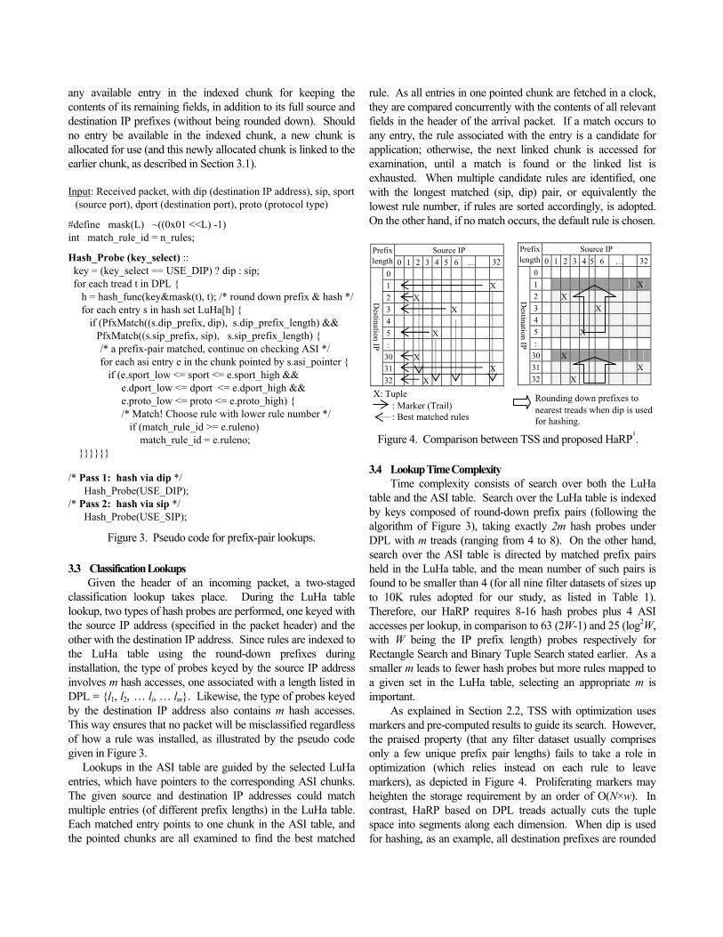
rule. As all entries in one pointed chunk are fetched in a clock, they are compared concurrently with the contents of all relevant fields in the header of the arrival packet. If a match occurs to any entry, the rule associated with the entry is a candidate for application; otherwise, the next linked chunk is accessed for examination, until a match is found or the linked list is exhausted. When multiple candidate rules are identified, one with the longest matched (sip, dip) pair, or equivalently the lowest rule number, if rules are sorted accordingly, is adopted. On the other hand, if no match occurs, the default rule is chosen.

Source IP Prefix length 0 1 2 3 4 5 6 … 32

0 1 X 2 X 3 X 4 5 X :

30 X 31 X

Destination IP

32 X X: Tuple : Marker (Trail) : Best matched rules

Source IP Prefix length 0 1 2 3 4 5 6 … 32

0 1 X 2 X 3 X 4 5 X :

30 X 31 X

Destination IP

32 X

Rounding down prefixes to nearest treads when dip is used for hashing.

Figure 4. Comparison between TSS and proposed HaRP1.

3.4 Lookup Time Complexity Time complexity consists of search over both the LuHa

table and the ASI table. Search over the LuHa table is indexed by keys composed of round-down prefix pairs (following the algorithm of Figure 3), taking exactly 2m hash probes under DPL with m treads (ranging from 4 to 8). On the other hand, search over the ASI table is directed by matched prefix pairs held in the LuHa table, and the mean number of such pairs is found to be smaller than 4 (for all nine filter datasets of sizes up to 10K rules adopted for our study, as listed in Table 1). Therefore, our HaRP requires 8-16 hash probes plus 4 ASI accesses per lookup, in comparison to 63 (2W-1) and 25 (log2W, with W being the IP prefix length) probes respectively for Rectangle Search and Binary Tuple Search stated earlier. As a smaller m leads to fewer hash probes but more rules mapped to a given set in the LuHa table, selecting an appropriate m is important.

As explained in Section 2.2, TSS with optimization uses markers and pre-computed results to guide its search. However, the praised property (that any filter dataset usually comprises only a few unique prefix pair lengths) fails to take a role in optimization (which relies instead on each rule to leave markers), as depicted in Figure 4. Proliferating markers may heighten the storage requirement by an order of O(N×w). In contrast, HaRP based on DPL treads actually cuts the tuple space into segments along each dimension. When dip is used for hashing, as an example, all destination prefixes are rounded

down to designated length specified by the DPL set, as demonstrated in Figure 4 for HaRPP

1 with designated prefix lengths equal to 30 and 1 shown. The selection of DPL can be made to match the distribution of unique prefix lengths for the best hashing results. Based on the fact that there are not many unique prefix pair length combinations [24, 25], HaRP design makes very efficient use of the LuHa table, in a way better than TSS over the tuple space. The storage requirement is a constant O(N), linear to the number of rules. 3.5 Handling Incremental Rule Updates and Additional Fields

HaRP admits dynamic filter datasets very well. Adding one rule to the dataset may or may not cause any addition to the LuHa table, depending upon if its (sip, dip) pair has been present therein. An entry from the ASI table will be needed to hold the remaining fields of the rule. Conversely, a rule removal requires only to make its corresponding ASI entry available. If entries in the affected ASI chunk all become free after this removal, its associated entry in the LuHa table is released as well.

Packet classification often involves many fields, subject to large dimensionality. As the dimension increases, the search performance of a TSS-based approach tends to degrade quickly while needed storage may grow exponentially due to the combinatorial specification of many fields. By contrast, adding fields under HaRP does not affect the LuHa table at all, and they only need longer ASI entries to accommodate them, without increasing the number of ASI entries. Search performance hence holds unchanged in the presence of additional fields.

4 Evaluation and Results This section evaluates HaRP using the publicly available

filter databases, focusing on the distribution results of prefix pairs in the LuHa table. Because the LuHa table is consulted 2m times for DPL with m treads, the distribution of prefix pairs plays a critical role in hashing performance. Our evaluation assumes a 4-way set-associative LuHa table design, with default DPL comprising 8 treads: {32, 28, 24, 20, 16, 12, 8, 1}, chosen conveniently, not necessary to yield the best results. It will show that our use of a single set-associative table obtained by collapsing individual hash tables (see Figure 1) is effective.

This work assumes overflows to be handled by linked lists, and each element in the linked list contains 4 entries able to hold 4 additional prefix pairs. HaRP is compared with other algorithms, including the Tuple Space Search, BV, and HyperCuts in terms of the storage requirement and measured execution time on a multi-core SoC.

4.1 Filter Datasets

Our evaluation employed the filter database suite from the open source of ClassBench [26]. The suite contains three seed filter sets: covering Access Control List (ACL1), Firewall (FW1), and IP Chain (IPC1), made available by service

providers and network equipment vendors. By their different characteristics, various synthetic filter datasets with large numbers of rules are generated in order to study the scalability of classification mechanisms. For assistance in, and validation on, implementation of different classification approaches, the filter suite is accompanied with traces, which can also be used for performance evaluation as well [29]. The filter datasets utilized by our study are listed in the following table.

Table 1. Filter datasets Seed Filters

(#filters, trace length)Synthetic Filters

(#filters, trace length) ACL1(752, 8140) ACL-5K(4415, 45600) ACL-10K(9603, 97000) FW1(269, 2830) FW-5K(4653, 46700) FW-10K(9311, 93250)

IPC1(1550, 17020) IPC-5K(4460, 44790) IPC-10K(9037, 90640)

4.2 Prefix Pair Distribution in LuHa Table The hash function is basic to HaRP. In this article, a

simple hash function is developed for use. First, a prefix key is rounded down to the nearest tread in DPL. Next, simple XOR operations are performed on the prefix key and the found tread length, as follows:

tread = find_tread_in_DPL(length of the prefix_key); pfx = prefix_key & (0xffffffff << (32-tread)); // round down h = (pfx) ^ (pfx>>7) ^ (pfx>>15) ^ tread ^ (tread<<5) ^ (tread<<12)^ ~(tread<<18) ^ ~(tread<<25); set_num = (h ^ (h >> 5) ^ (h<<13)) % num_of_set;

While better results may be achieved by using more sophisticated hash functions (such as cyclic redundancy codes, for example), it is beyond the scope of this article. Instead, we show that a single lumped LuHa table can be effective, and most importantly, HaRP* works satisfactorily under a simple hash function.

The results of hashing prefix pairs into the LuHa table are shown in Figure 5, where the LuHa tables are properly sized. Specifically, the LuHa table is provisioned with ρ = 2 (dilated by a factor of 2 relative to the number of filter rules) for HaRP1, whereas its size is then reduced by 25% (i.e., ρ = 1.5) to show how the single set-associative LuHa table performs with respect to fewer treads in DPL under HaRP*. Figure 5(a) illustrates that HaRP1 exhibits no more than 4% of overflowing sets in a 4-way set-associative LuHa table. Note that those results for 5K filter datasets (i.e., ACL-5K, FW-5K, and IPC-5K) were omitted in Figure 5 so that the remaining 6 curves can be read more easily, given that those omitted results lying between the set of results for 1K filter datasets and that for 10K datasets. Only the IPC1 dataset happens to have 20 prefix pairs mapped into one set. This congested set is caused partly by the non-ideal hash function and partly by the round-down mechanism of HaRP. Nevertheless, the single 4-way LuHa table exhibits good resilience in accommodating hash collisions for the vast majority (96%) cases.

When the number of DPL treads is reduced to 6 under HaRP*, improved and well-balanced results can be observed in

Figure 5. Results of hashing round-down prefixes into LuHa table.

(a)

(c)

HaRP*, with dilation factor = 1.5 and DPL of 6 treads

0%

20%

40%

60%

80%

100%

0 1 2 3 4 5 6 7 8 9 10 11 12 13

Number of Prefix Pairs in a Set

Per

cent

age(

/Tot

al S

ets)

FW1

ACL1

IPC1

FW-10K

ACL-10K

IPC-10K

(d)

HaRP1, with dilation factor = 2 and DPL of 8 treads

0%

20%

40%

60%

80%

100%

0 1 2 3 4 5 6 7 8 9 10 11 12 13 14 15 16 17 18 19 20

Number of Prefix Pairs in a Set

Per

cent

age(

/Tot

al S

ets)

FW1

ACL1

IPC1

FW-10K

ACL-10K

IPC-10K

(b)

HaRP*, with dilation factor = 1.5 and DPL of 4 treads

0%

20%

40%

60%

80%

100%

0 1 2 3 4 5 6 7 8 9 10 11 12 13

Number of Prefix Pairs in a Set

Per

cent

age(

/Tot

al S

ets)

FW1

ACL1

IPC1

FW-10K

ACL-10K

IPC-10K

HaRP*, with dilation factor = 2 and DPL of 6 treads

0%

20%

40%

60%

80%

100%

0 1 2 3 4 5 6 7 8 9 1

Number of Prefix Pairs in a Set

Per

cent

age(

/Tot

al S

ets)

0

FW1

ACL1

IPC1

FW-10K

ACL-10K

IPC-10K

Figure 5(b), where ρ equal 2. All datasets now experience less than 1% overflowing sets, except for ACL1 and IPC1 (which have some 4% and 8% overflows, respectively). Noticeably, even the most punishing case of IPC1 encountered in Figure 5(a) is reassured. These desirable results hold true when the LuHa table size is reduced by 25% and DPL contains fewer thread, as shown in Figures 5(c) and 5(d). Although a few congested sets emerge, they are still manageable. With 6 treads in DPL, fewer congested sets, albeit marginal, occur, as demonstrated in Figure 5(c), than with 4 threads depicted in Figure 5(d). This is expected, since the hash values are calculated over round-down prefixes, and a less number of treads leads to wider strides between consecutive treads, likely to make more prefixes identical in hash calculation after being rounded down. Furthermore, fewer treads in DPL implies a smaller number of LuHa table candidate sets among which prefix pairs can be stored. These results indicate that a single lumped set-associative table for HaRP* is promising in accommodating prefix pairs of filter rules in a classification dataset effectively.

4.3 Search over ASI Table

The second stage of HaRP probes the ASI (application-specific information) table, each of whose entry holds values of all remaining fields, as illustrated in Figure 1. As LuHa table

search has eliminated all rules whose source and destination IP prefixes do not match, pointing solely to those candidate ASI entries for further examination. It is important to find out how many candidate ASI entries exist for a given incoming packet, as they govern search complexity involved in the second stage.

As described in Section 3.1, we adopt a very simple design which puts rules with the same prefix pairs in an ASI chunk. While a more optimized design with smaller storage and higher lookup performance may be achieved by advanced techniques and data structures, we study the effectiveness of HaRP by using basic linear lists because of its simplicity.

The ASI lists are generally short, as shown in Figure 6, where the results for 5K filter datasets were omitted again for clarity. Over 95% of them have less than 5 ASI entries each, and hence, linear search is adequate. The ACL1 dataset is an exception, experiencing a long ASI list with 36 entries. By scrutinizing the outcome, we found that this case is caused by a large number of rules specified for a specific host pair, leading to a poor case since those rules for such host pairs fall in the same list. Furthermore, those rules have the form of (0:max_destination_port, ×, tcp), that is, a range is specified for the destination port, with the source port being wild carded and the protocol being TCP. Importantly, the destination port range (0, dpi) for Rule i is a sub-range of (0, dpi+1) for Rule i+1. This is believed to

represent a situation where a number of applications at the target host rein accesses from a designated host. Nevertheless, fetching all ASI entries within one chunk at a time (achievable by placing them in the same word line) helps to address long ASI lists, if present (since one ASI chunk may easily accommodate 8 entries, each with 80 bits, as stated in the next subsection).

Note that the ASI distribution is orthogonal to the selection of DPL and to the LuHa table size. Filter rules are put in the same ASI list only if they have the same prefix pair combination.

4.4 Storage Requirements Table 2 shows memory storage measured for the rule

datasets. Each LuHa entry is 12-byte long, comprising two 32b IP address prefixes, two 5b prefix length indicators, a 16b pointer to the ASI table, and a 6b integer indicating the length of its associated linked list. Each ASI entry needs 10 bytes to keep the port ranges and the protocol type, plus two bytes for the rule number (i.e., the priority).

Table 2. Memory size

Total Storage (in KB, or

otherwise MB as specified) Per Rule Storage(Byte, or otherwise KB as specified)

HaRP Tuple Space BV Hyper-

Cuts HaRP TupleSpace BV Hyper

-Cuts

FW1 4.64 22.72 10.50 10.19 17.66 86.49 40 36.79

ACL1 13.79 44.19 52.14 20.24 18.78 60.18 71 25.56

IPC1 29.17 56.26 92.33 91.19 19.27 37.17 61 58.25

FW-5K 101.0 629.5 3.07M 4.10M 22.23 138.5 691 922.3

ACL-5K 76.54 157.7 1.08M 136.8 17.75 36.57 257 29.73

IPC-5K 90.56 199.4 1.52M 332.6 20.79 45.79 358 74.34

FW-10K 217.3 1.68M 14.05M 25.05M 23.9 189.2 1.54K 2.75K

ACL-10K 192.5 403.4 7.31M 279.4 20.52 43.02 798 27.79

IPC-10K 187.5 449.8 6.79M 649.5 21.24 50.97 788 71.60

As listed in Table 2, HaRP enjoys clear superiority

when compared with its previous counterparts, whose implemented source codes were available publicly [29] and

employed to gather their respective results included here. HaRP dramatically reduces memory storage needed and demonstrates consistent levels of storage requirement across all datasets examined. Previous techniques, especially those using decision-tree- or trie-based algorithms, exhibit rather unpredictable outcomes because the size of a trie largely depends on if datasets have comparable prefixes to enable trie contraction; otherwise, a trie can grow quickly toward full expansion. Among prior techniques, tuple space search (TSS) [24] and HyperCuts [20] show better results, although they still require more memory than HaRP. Those listed outcomes generally indicate what can be best achieved by the cited techniques. For TSS, as an instance, Tuple Pruning is implemented, but not pre-computed markers which increase storage requirement (see Section 2.2 and Figure 4 for details). For HyperCuts, its refinement options are all turned on, including rule overlapping and rule pushing for the most optimization results [20].

0%

10%

20%

30%

40%

50%

60%

70%

80%

90%

100%

1 2 3 4 5 6 7 8 9 10 11 12 13 14 15+Num. of ASI Entries per List

Perc

enta

ge(/T

otal

ASI

ent

ries)

FW1

ACL1

IPC1

FW-10K

ACL-10K

IPC-10K

Figure 6. Length distribution of ASI link lists.

The results of memory efficiency, defined as the ratio between the total storage of constituent data structures (which include the provisioned but not occupied entries for the LuHa table in HaRP) and the minimal storage required to keep all filter rules (as in a linear array of rules), for various algorithms are listed in Table 3.

Table 3. Memory efficiency

HaRP (ρ = 2)

HaRP (ρ = 1.5)

Tuple Space BV Hyper-

Cuts FW1 1.62 1.35 3.60 1.67 1.93

ACL1 1.58 1.31 2.51 2.96 1.38 IPC1 1.58 1.31 1.55 2.54 3.01

FW-5K 1.59 1.32 5.77 28.83 46.21 ACL-5K 1.58 1.31 1.52 10.69 1.59 IPC-5K 1.58 1.31 1.91 14.89 3.82 FW-10K 1.58 1.31 7.88 65.93 141.0 ACL-10K 1.58 1.31 1.79 33.26 1.49 IPC-10K 1.59 1.37 2.12 32.83 3.68

There are a number of interesting findings. First of all,

HaRP consistently delivers greater efficiency than all other algorithms. When the LuHa table is dilated by a factor ρ = 2, all memory data structures allocated are no more than 50% of the amount required to keep the rules. If the LuHa table size is reduced to ρ = 1.5, total storage drops by 25%. In general, a smaller LuHa table yields lower performance because of more hash collisions. However, the next section will show measured results on multi-core systems under a small LuHa table (with ρ = 1.5) and small DPL to deliver satisfactory performance comparable to that under larger tables.

Contrary to HaRP enjoying consistent efficiency always, all other methods exhibit unsteady results. When the number of filter rules is small, those methods may achieve reasonable memory efficiency. As the dataset size grows, their efficiency results vary dramatically. For HyperCuts [20] (which uses a multi-way branch trie), its size largely depends on if datasets

have comparable prefixes that enable trie contraction; otherwise, the trie can grow exponentially toward full expansion. A decision tree-based method suffers from the fact that its number of kept rules may blow up quickly under a filter dataset with plentiful wild-carded rules. The less specific filter rules are, the lower memory efficiency it becomes, because a wild-carded rule holds true for all children at a node irrespective of the number of branches (cuts) made therein. (We have seen consistent trends for large datasets comprising 20K and 30K rules generated using the tool included in the ClassBench [26].) As analyzed in Section 3.1 and shown in Figure 2, the FW applications have over 60% wild-carded IP addresses (versus some 0.1% to 8% for ACL and IPC), yielding the worst memory efficiency consistently in Table 3. To a large degree, TSS [24] and BV [13] also leverage tries to narrow the search scope and hence are subject to the same problem. Furthermore, TSS employs one hash table per tuple in the space, likely to bloat the memory size because of underutilized hash tables. For BV, the n-bit vector stored at each leaf node of a trie is the main culprit for being memory guzzler.

Section 5.2 will demonstrate the measured performance results of HaRP, revealing that it not only achieves the best memory efficiency among all known methods but also classifies packet at four times faster than HyperCuts, and an order of magnitude higher than TSS and BV, under our multi-core evaluation platform.

5 Scalability and Lookup Performance on Multi-Cores As each packet can be handled independently, packet

classification suits a multi-core system well [6]. Given a multi-core processor with np cores, a simple implementation may assign a packet to any available core at a time so that np packets can be handled in parallel by np cores.

In this section, we present and discuss performance and scalability of HaRP in comparison with those of its counterparts BV [13], TSS [24], and HyperCuts [20]. Two HaRP configurations are considered: (1) basic HaRP with the LuHa table under a dilation factor ρ = 2 and with 8 treads in DPL, and (2) HaRP* with the LuHa table under ρ = 1.5 and with only 4 treads in DPL. By comparing results obtained for basic HaRP and HaRP*, we can gain insight into how the LuHa table size and the number of treads affect lookup performance.

For gathering measures of interest on our multi-core platform, our HaRP code was made multithreaded for execution. With those source codes for BV, TSS and HC implementations taken from the public source [29], we closely examined and polished them by removing unneeded data structures and also replacing some poor code segments with in order to get best performance levels of those referenced techniques. All those program codes were also made multithreaded to execute on the same multi-core platform, with their results presented in next sections.

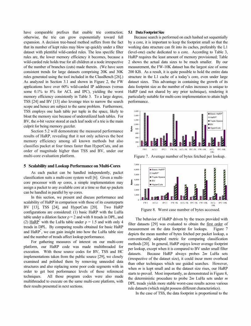
5.1 Data Footprint Size Because search is performed on each hashed set sequentially

by a core, it is important to keep the footprint small so that the working data structure can fit into its caches, preferably the L1 (level-one) cache dedicated to a core. According to Table 3, HaRP requires the least amount of memory provisioned; Table 2 shows the actual data sizes to be much smaller. By our measurement, the FW-10K dataset has the largest size of some 200 KB. As a result, it is quite possible to hold the entire data structure in the L1 cache of a today’s core, even under large dataset sizes. This advantage in containing the growth of its data footprint size as the number of rules increases is unique to HaRP (and not shared by any prior technique), rendering it particularly suitable for multi-core implementation to attain high performance.

0

200

400

600

800

1,000

1,200

1,400

1,600

FW1 ACL1 IPC1 FW-5K ACL-5K IPC-5K FW-10K ACL-10K

IPC-10K

Byt

es

Basic HaRP

HaRP*

Tuple Space

BV

HyperCuts

Figure 7. Average number of bytes fetched per lookup.

0

1,000

2,000

3,000

4,000

5,000

6,000

7,000

FW1 ACL1 IPC1 FW-5K ACL-5K IPC-5K FW-10K ACL-10K

IPC-10K

Byt

es

Basic HaRP

HaRP*

Tuple Space

BV

HyperCuts

Figure 8. Worst case number of bytes accessed.

The behavior of HaRP driven by the traces provided with filter datasets [29] was evaluated to obtain the first order of measurement on the data footprint for lookups. Figure 7 depicts the mean number of bytes fetched per packet lookup, a conventionally adopted metric for comparing classification methods [20]. In general, HaRP enjoys lower average footprint per lookup, except when it is compared to BV under small filter datasets. Because HaRP always probes 2m LuHa sets (irrespective of the dataset size), it could incur more overhead than other techniques which use guided searches. However, when m is kept small and as the dataset size rises, our HaRP starts to prevail. Most importantly, as demonstrated in Figure 8, the deterministic procedure to probe 2m LuHa sets under m DPL treads yields more stable worst-case results across various rule datasets (which might possess different characteristics).

In the case of TSS, the data footprint is proportional to the

num

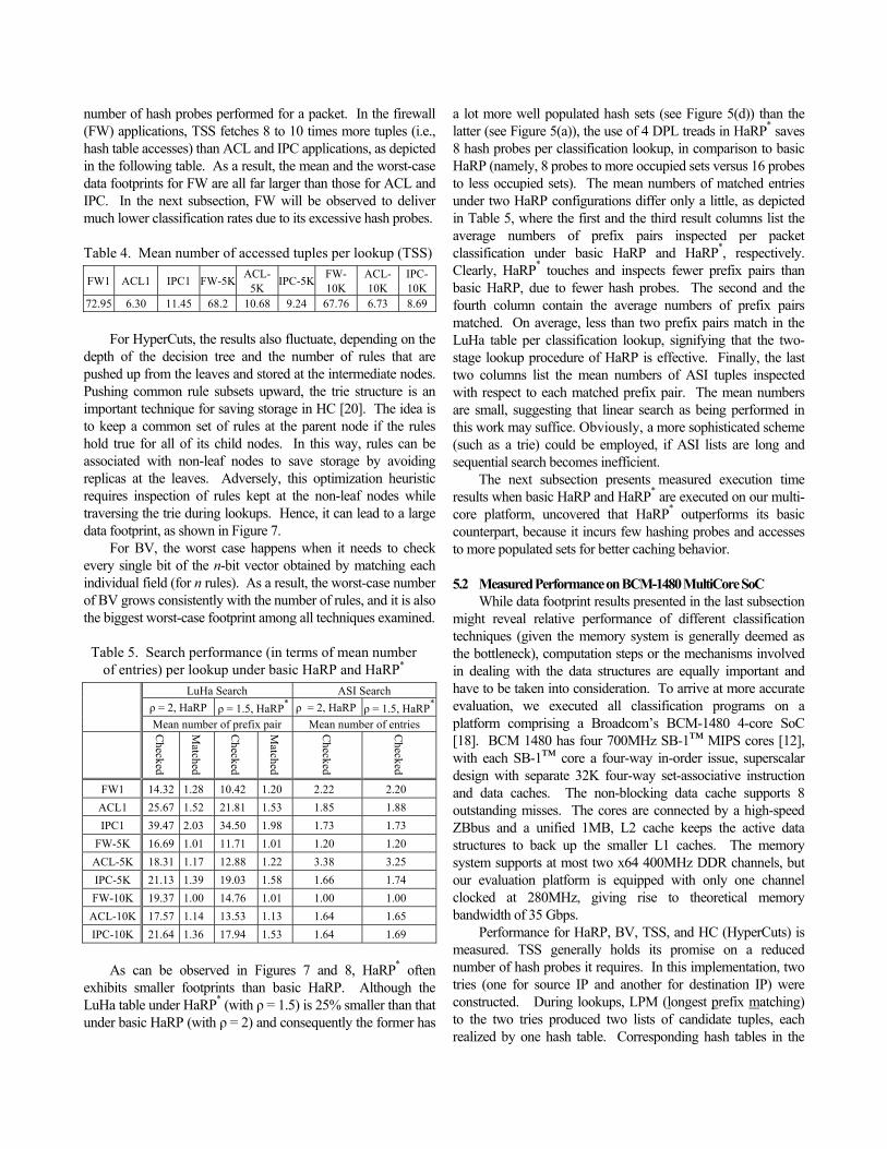
Table 4. Mean number of accessed tuples per lookup (TSS)

ber of hash probes performed for a packet. In the firewall (FW) applications, TSS fetches 8 to 10 times more tuples (i.e., hash table accesses) than ACL and IPC applications, as depicted in the following table. As a result, the mean and the worst-case data footprints for FW are all far larger than those for ACL and IPC. In the next subsection, FW will be observed to deliver much lower classification rates due to its excessive hash probes.

FW1 ACL1 IPC1 FW-5K ACL- IPC-5K FW- ACL- IPC-5K 10K 10K 10K

72.95 6.30 11.45 68.2 1 0.68 9.24 67.76 6.73 8.69 For HyperCuts, the results also fluctuate, depending on the

dept

en it needs to check ever

Table 5. Search performance (in terms of mean number

h of the decision tree and the number of rules that are pushed up from the leaves and stored at the intermediate nodes. Pushing common rule subsets upward, the trie structure is an important technique for saving storage in HC [20]. The idea is to keep a common set of rules at the parent node if the rules hold true for all of its child nodes. In this way, rules can be associated with non-leaf nodes to save storage by avoiding replicas at the leaves. Adversely, this optimization heuristic requires inspection of rules kept at the non-leaf nodes while traversing the trie during lookups. Hence, it can lead to a large data footprint, as shown in Figure 7.

For BV, the worst case happens why single bit of the n-bit vector obtained by matching each

individual field (for n rules). As a result, the worst-case number of BV grows consistently with the number of rules, and it is also the biggest worst-case footprint among all techniques examined.

of entries) per lookup under basic HaRP and HaRP*

LuHa Search ASI Search ρ = 2, H HaRP* ρ = 2, H , HaRP*aRP ρ = 1.5, aRP ρ = 1.5 Mean number of prefix pair Mean number of entries

Checked

Ma

Matched

Checked

tched

Checked

Checked

FW1 1 1 1 2 214.32 .28 0.42 .20 .22 .20 ACL1 25.67 1.52 21.81 1.53 1.85 1.88 IPC1 39.47 2.03 34.50 1.98 1.73 1.73

F W-5K 16.69 1.01 11.71 1.01 1.20 1.20 ACL-5K 18.31 1.17 12.88 1.22 3.38 3.25 IPC-5K 21.13 1.39 19.03 1.58 1.66 1.74 FW-10K 19.37 1.00 14.76 1.01 1.00 1.00

ACL-10K 17.57 1.14 13.53 1.13 1.64 1.65 IPC-10K 21.64 1.36 17.94 1.53 1.64 1.69

As can be observed in Figures 7 and 8, HaRPP

* often exhibits smaller footprints than basic HaRP. Although the LuHa table under HaRP* (with ρ = 1.5) is 25% smaller than that under basic HaRP (with ρ = 2) and consequently the former has

a lot more well populated hash sets (see Figure 5(d)) than the latter (see Figure 5(a)), the use of 4 DPL treads in HaRPP

* saves 8 hash probes per classification lookup, in comparison to basic HaRP (namely, 8 probes to more occupied sets versus 16 probes to less occupied sets). The mean numbers of matched entries under two HaRP configurations differ only a little, as depicted in Table 5, where the first and the third result columns list the average numbers of prefix pairs inspected per packet classification under basic HaRP and HaRP*

P

easured execution time resu

, respectively. Clearly, HaRP* touches and inspects fewer prefix pairs than basic HaRP, due to fewer hash probes. The second and the fourth column contain the average numbers of prefix pairs matched. On average, less than two prefix pairs match in the LuHa table per classification lookup, signifying that the two-stage lookup procedure of HaRP is effective. Finally, the last two columns list the mean numbers of ASI tuples inspected with respect to each matched prefix pair. The mean numbers are small, suggesting that linear search as being performed in this work may suffice. Obviously, a more sophisticated scheme (such as a trie) could be employed, if ASI lists are long and sequential search becomes inefficient.

The next subsection presents mlts when basic HaRP and HaRP* are executed on our multi-

core platform, uncovered that HaRPP

5.2 Measured Performance on BCM-1480 MultiCore SoC ection

migh

P, BV, TSS, and HC (HyperCuts) is mea

* outperforms its basic counterpart, because it incurs few hashing probes and accesses to more populated sets for better caching behavior.

While data footprint results presented in the last subst reveal relative performance of different classification

techniques (given the memory system is generally deemed as the bottleneck), computation steps or the mechanisms involved in dealing with the data structures are equally important and have to be taken into consideration. To arrive at more accurate evaluation, we executed all classification programs on a platform comprising a Broadcom’s BCM-1480 4-core SoC [18]. BCM 1480 has four 700MHz SB-1™ MIPS cores [12], with each SB-1™ core a four-way in-order issue, superscalar design with separate 32K four-way set-associative instruction and data caches. The non-blocking data cache supports 8 outstanding misses. The cores are connected by a high-speed ZBbus and a unified 1MB, L2 cache keeps the active data structures to back up the smaller L1 caches. The memory system supports at most two x64 400MHz DDR channels, but our evaluation platform is equipped with only one channel clocked at 280MHz, giving rise to theoretical memory bandwidth of 35 Gbps.

Performance for HaRsured. TSS generally holds its promise on a reduced

number of hash probes it requires. In this implementation, two tries (one for source IP and another for destination IP) were constructed. During lookups, LPM (longest prefix matching) to the two tries produced two lists of candidate tuples, each realized by one hash table. Corresponding hash tables in the

3.7 5.03.2 3.9 5.1

4.53.9 4.3

4.0

2.4 3.42.5

2.4 3.63.3

2.4 3.02.9

0246810121416182022

Rel

ativ

e Sc

ale

to H

yper

Cut

s(1)

FW1

AC

L1

IPC

1FW

1-5K

AC

L1-5

K

IPC

1-5K

FW1-

10K

AC

L1-1

0K

IPC

1-10

K

BV

(1)

BV

(2)

BV

(4)

Hyp

erC

uts(

1)

Tupl

e(1)

HaR

P(1

)

HaR

P*(

1)

Hyp

erC

uts(

2)

Tupl

e(2)

HaR

P(2

)

HaR

P*(

2)

Hyp

erC

uts(

4)

Tupl

e(4)

HaR

P(4

)

HaR

P*(

4)

BV(1) BV(2) BV(4)HyperCuts(1) Tuple(1) HaRP(1)HaRP*(1) HyperCuts(2) Tuple(2)HaRP(2) HaRP*(2) HyperCuts(4)Tuple(4) HaRP(4) HaRP*(4)

Figure 9. Measured throughput results on Broadcom BCM-1480 4-core SoC (in relative scale).

intersection of the two lists (namely, intersected tuples) are then probed. All executed programs were made multithreaded such that up to 4 threads could be launched to take advantage of the 4 SB-1TM cores. Millions of packets were generated from the traces packaged together with the rule datasets to measure the real elapsed times via the BCM-1480 ZBus counter, which ticks at every system clock.

Results depicted in Figure 9 are all relatively scaled to one thread HyperCuts performance, which is shown as a consistent scal

2.4 t

stemming from the fact it employs DPL

e of one across the graph for clear and system configuration-independent comparison. Labels on the x-axis of Figure 9 denote different techniques (i.e., BV, HyperCuts, TSS, and HaRP) executed on varying numbers of BCM-1480 cores (i.e., 1, 2, and 4). For example, BV(2) (or Tuple(4)) refers to BV (or TSS) run on 2 (or 4) cores. When the number of threads rises from 1 to 2 and then 4, HC shows a nearly linear scalability (in terms of raw classification rates) with respect to the number of cores. This scalability trend indeed exists for all techniques because packet classification is inherently parallel, as expected.

Overall, HaRP demonstrates the highest throughput among all techniques. On a per core basis, HaRP consistently delivers

o 3.5 times improvement over HC under the nine filter datasets. When compared with TSS, basic HaRP performs 2 to 3 times better than TSS under ACL and IPC filter datasets, and 8 times under the firewall applications (FWs). This is because HaRP requires fewer hash probes than TSS under firewall datasets. Our HaRP always performs 2m lookups, equal to 16 for m = 8. Contrary to HaRP, TSS performs as many as four times more hash probes under Firewall (see Table 4). For ACL and IPC datasets, TSS may require slightly fewer hash table lookups, but that advantage is more than negated by its two LPM search passes over the tries, with respect to the source and the destination IP prefixes. Furthermore, the smaller data footprint enjoyed by HaRP (demonstrated in Figure 7) leads to better cache performance.

Relative performance exhibited by HaRP* is even greater than that by basic HaRP,

with 4 treads, as opposed to 8 treads for HaRP. This brings the number of hash probes per lookup from 16 down to 8, incurring less hashing overhead. Most importantly, HaRPP

* is expected to be more caching-friendly, because accessing prefix pairs located in 8 sets should enjoy better caching locality than prefix pairs spread across 16 sets. Even though HaRP*

P uses a LuHa table which is 25% smaller than that of HaRP, HaRPP

it sta

ent filter

m that TSS can outperform HC in such a wide ma

* outperforms HC (or TSS) by 4 to 5 times (or 3 to 10 times), on an average, under the nine datasets, as demonstrated in Figure 9.

When compared to HC, BV shows poor performance with O(10) degradation, especially for large filter datasets. Because

rts with five LPM search processes across separate tries for individual header fields to produce a list of candidate rules in order to get a 5-field cross product, BV is inefficient for software implementation run on a multi-core platform, since its processor caches are expected to be trashed due to the large footprint incurred, as revealed in Figures 7 and 8. Thus, BV is better suitable for custom hardware with parallelism supported by high memory bandwidth, suffering from poor scalability.

Table 4 lists the average number of tuples (i.e., hash tables) fetched per packet lookup under TSS, with respect to differ

datasets examined. Hash probes for firewall applications (FWs) are far more than those for ACL and IPC datasets. This is consistent with the results of Figures 7 and 8, where FWs exhibit large footprints. Under FWs, TSS delivers 50% to 70% less performance than HC on a per-core basis. However, TSS outperforms HC under ACL and IPC datasets by as much as nearly 100%.

According to the average footprint results given in Figure 7, it does not see

rgin. For ACL-5K and ACL-10K datasets, HC reads roughly the same amount (but no more than 10%) of data bytes as TSS. However, TSS delivers almost 100% higher

throughputs per core. Under IPC-5K and IPC-10K, TSS fetches about 50% less data than HC and shows 47% higher throughput. It confirms that the data footprint can indeed give first-order estimation on how well a technique could perform, but the code path during execution is nevertheless critical. By inspecting the disassembled HC code, we found that the code path for HC could be long. For example, at each step traversing the decision tree, the number of bits to be extracted from a field needs to be determined, and next the extracted bits are used to calculate the location of the next child in the decision tree. In brief, the total number of splits (i.e., children) of a node is specified by NC = Πi nc(i), where nc(i) is the number of cuts performed on the ith header field. During search, log2(nc(i)) bits are extracted from the appropriate positions in the ith field; assuming the decimal value represented by the extracted bits is vi, the number of child positions in the linear array covering the

NC space is then expressed by DD

ij

D

ii vjncv +Π×∑

+=

−

=)(

1

1

1 for D

dimensions. These operations seem hey can take hundreds of cycles to com ificant performance loss, as observed above.

simple, but in fact, tplete, causing a sign

6 Concluding Remarks Packet classification is

functionality and services, bessential for most network system ut it is complex since it involves

comparing multiple fields in a packet header against entries in the filter dataset to decide the proper rule to apply for handling the packet [9]. This article has considered a rapid packet classification mechanism realized by hashing round-down prefixes (HaRP) able to not only exhibit high scalability in terms of both the classification time and the SRAM size involved, but also effectively handle incremental updates to the filter datasets. Based on a single set-associative LuHa hash table (obtained by lumping a set of hash table units together) to support two-staged search, HaRP promises to enjoy better classification performance than its known software-oriented counterpart, because the LuHa table narrows the search scope effectively based on the source and the destination IP addresses of an arrival packet during the first stage, leading to fast search in the second stage. With its required SRAM size lowered considerably, HaRP makes it possible to hold entire search data structures in the local cache of each core within a contemporary processor, further elevating its classification performance.

The LuHa table admits each filter rule in a set with lightest occupancy among all those indexed by hash(round-down sip) and hash(round-down dip), under HaRPP

has

HaRP , as we have witn

and M. Mitzenmacher, “Using Multiple Hash o Improve IP Lookups,” Proceedings of 20th Annual

[2] k Processors and

[3] ernational

[4] ings of 12

[5] Proc. of IEEE Int’l Conf. on

[6] ACM

*. This lowers substantially the likelihood of set overflow, which occurs only when all indexed sets are full, attaining high SRAM storage utilization. It also leads to great scalability, even for small LuHa table set-associativity (of 4), as long as the table is dilated by a small factor (say, ρ = 1.5 or 2). Our evaluation results have shown that HaRP* with the set associative degree of 4, generally experiences very rare set overflow instances (i.e., no more than

1% of those sets in the LuHa table with ρ = 2 under all studied filter datasets other than ACL1 and IPC1, if DPL has 6 treads).

Empirical assessment of HaRP has been conducted on our platform comprising a Broadcom’s BCM-1480 SoC [18], which

four 700MHz SB-1TM MIPS cores [12]. A simple hashing function was employed for our HaRP implementation. Extensive measured results demonstrate that HaRP* outperforms HC [20] (or TSS [24]) by 4 to 5 times (or 3 to 10 times), on an average, under the nine databases examined, when its LuHa table is with ρ = 1.5 and there are 4 DPL treads. Besides its efficient support for incremental rule updates, our proposed HaRP also enjoys far better classification performance than previous software-based techniques.

Note that theoretically pathological cases may occur despite encouraging pragmatic results by *

essed in this study. For example, a large number of (hosts on the same subnet with) prefixes P|w can differ only in a few bits. Hence, those prefixes can be hashed into the same set after being rounded down, say P|w to P|li, for li ≤ w < li+1, under HaRP*. There are possible ways to deal with such cases and to avoid overwhelming the indexed set. A possible means is to use one and only one entry to keep the round-down prefix P|li, as opposed to holding all P|w’s in individual entries following the current design. Subsequently, the (w - li) round-down bits can form a secondary indexing structure to provide the differentiation (among rules specific to each host) and/or the round-down bits can be mingled with the remaining fields of the filter rules. Thus, each stage narrows the range of search by small and manageable structures. These possible options will be explored in the future.

References [1] A. Broder

Functions tJoint Conf. of IEEE Computer and Communications Societies (INFOCOM 2001), pp. 1454–1463, Apr. 2001. F. Chang et al., “Efficient Packet Classification with Digest Caches,” Proceedings of Workshop on NetworApplications (NP-3, in conjunction with 10th Int’l Conference on High-Performance Computer Architecture), Feb. 2004. W. T. Chen, S. B. Shih, and J. L. Chiang, “A Two-Stage Packet Classification Algorithm,” Proceedings of 17th IntConference on Advanced Information Networking and Applications (AINA ’03), pp. 762-767, Mar. 2003. Y. H. Cho and W. H. Magione-Smith, “Deep Packet Filter with Dedicated Logic and Read Only Memories,” Proceed th

IEEE Symposium on Field-Programmable Custom Computing Machines, pp. 125-134, Apr. 2004. Y.-T. Chen and S.-S. Lee, “An Efficient Packet Classification Algorithm for Network Processors,”Communications (ICC 2003), pp. 1596-1600, May 2003. H. Cheng et al., “Scalable Packet Classification Using Interpreting a Cross-Platform Multi-Core Solution,” Proceedings 13th

SIGPLAN Symposium on Principles and Practice of Parallel

Programming (PPoPP ’08), pp. 33-42, Feb. 2008. S. Dharmapurikar et al., “Fast Packet Classification Using Bloom Filters,” Proc. ACM/IEEE Symp. Architectures fo

[7] r Networking

[8]

[9] Conference of Special

[10] ings,” IEEE Micro, vol. 20, pp. 34-41,

[11] on Hardware Accelerator,” Proceedings of IEEE

[12] ,” Proceedings of IEEE Symp.

[13] l Range

[14] Advanced Packet Classification with Ternary

[15] earch,” Computer Networks, vol. 50, pp.

[16] urnal on Selected Areas in

[17] E Conf.

[18]

and Communications Systems (ANCS ’06), pp. 61-70, Dec. 2006. Q. Dong et al., “Wire Speed Packet Classification without TCAMs: A Few More Registers (and a Bit of Logic) Are Enough,” Proceedings of ACM International Conference on Measurement and Modeling of Computer Systems (SIGMETRICS ’07), pp. 253-264, June 2007. P. Gupta and N. McKeown, “Packet Classification on Multiple Fields,” Proceedings of ACM Annual Interest Group on Data Communication (SIGCOMM ’99), pp. 147-160, Aug./Sept. 1999. P. Gupta and N. McKeown, “Classifying Packets with Hierarchical Intelligent CuttJan. 2000. A. Kennedy, X. Wang, and B. Liu, “Energy Efficient Packet ClassificatiInternational Symposium on Parallel and Distributed Processing (IPDPS 2008), pp. 1-8, Apr. 2008. D. Kruckemyer, “The SB-1TM Core: A High Performance, Low Power MIPSTM 64 Implementationon High Performance Chips (Hot Chips 12), Aug. 2000. T. V. Lakshman and D. Stiliadis, “High-Speed Policy-Based Packet Forwarding Using Efficient Multi-DimensionaMatching,” Proc. of ACM Annual Conference of Special Interest Group on Data Communication (SIGCOMM ’98), pp. 191-202, Aug./Sept. 1998. K. Lakshminarayanan, A. Rangarajan, and S. Venkatachary, “Algorithms for CAMs,” Proceedings of ACM Annual Conference of Special Interest Group on Data Communication (SIGCOMM 2005), pp. 193-204, Aug. 2005. F.-Y. Lee and S. Shieh, “Packet Classification Using Diagonal-Based Tuple Space S1406-1423, 2006. J. van Lunteren and T. Engbersen, “Fast and Scalable Packet Classification,” IEEE JoCommunications, vol. 21, no. 4, pp. 560-571, May 2003. F. Pong and N.-F. Tzeng, “Storage-Efficient Architecture for Routing Tables via Prefix Transformation,” Proc. 32nd IEEon Local Computer Networks (LCN 2007), pp. 55-62, Oct. 2007. S. Santhanam et al., “A 1GHz Power Efficient Single Chip Multiprocessor System for Broadband Networking Applications,”Proc. of 15th Symp. on VLSI Circuits, June 2001, pp. 107-110.

[19] D. Shah and P. Gupta, “Fast Incremental Updates on Ternary-CAMs for Routing Lookups and Packet Classification,” Proc. of 8th Annual IEEE Symposium on High-Performance Interconnects (Hot Interconnects 8), pp. 145-153, Aug. 2000.

[20] S. Singh et al., “Packet Classification using Multidimensional Cutting,” Proceedings of ACM Annual Conference of Special Interest Group on Data Communication (SIGCOMM 2003), pp. 213-114, Aug. 2003.

[21] H. Song and J. W. Lockwood, “Efficient Packet Classification for Network Intrusion Detection Using FPGA,” Proceedings of ACM/SIGDA 13th International Symposium on Field Programmable Gate Arrays (FPGA ’05), pp. 238-245, Feb. 2005.

[22] E. Spitznagel, D. Taylor, and J. Turner, “Packet Classification Using Extended TCAMs,” Proceedings of 11th IEEE Int’l Conf. on Network Protocols (ICNP ’03), pp. 120-131, Nov. 2003.

[23] V. Srinivasan et al., “Fast and Scalable Layer Four Switching,” Proc. of ACM Annual Conference of Special Interest Group on Data Communication (SIGCOMM ’98), pp. 191-202, Sept. 1998.

[24] V. Srinivasan, S. Suri, and G. Varghese, “Packet Classification Using Tuple Space Search,” Proceedings of ACM Annual Conference of Special Interest Group on Data Communication (SIGCOMM ’99), pp. 135–146, Aug./Sept. 1999.

[25] D. E. Taylor, “Survey and Taxonomy of Packet Classification Techniques,” ACM Computing Surveys, vol. 37, no. 3, pp. 238-275, Sept. 2005.

[26] D. E. Taylor and J. S. Turner, “ClassBench: A packet Classification Benchmark,” Proc. 24th IEEE Int’l Conference on Computer Communications (INFOCOM 2005), March 2005.

[27] G. Wang and N.-F. Tzeng, “TCAM-Based Forwarding engine with Minimum Independent Prefix Set (MIPS) for Fast Updating,” Proceedings of IEEE International Conference on Communications (ICC ’06), June 2006.

[28] P. Warkhede, S. Suri, and G. Varghese, “Fast Packet Classification for Two-Dimensional Conflict-Free Filters,” Proc. 20th Annual Joint Conf. of IEEE Computer and Communications Societies (INFOCOM 2001), pp. 1434–1443, Apr. 2001.

[29] Washington University, “Evaluation of Packet Classification Algorithms,” at http://www.arl.wustl.edu/~hs1/PClassEval.html.

[30] Z. Wu, M. Xie, and H. Wang, “Swift: A Fast Dynamic Packet Filter,” Proceedings of 5th USENIX Networked Systems Design and Implementation (NSDI ’08), pp. 279-292, Apr. 2008.