Hartree -Fock Theoryatlas.physics.arizona.edu/~shupe/Indep_Studies... · Hartree -Fock...

Lecture 7Lecture 7

HartreeHartree--Fock TheoryFock Theory

WS2012/13WS2012/13: : ‚‚Introduction to Nuclear and Particle PhysicsIntroduction to Nuclear and Particle Physics‘‘, Part I, Part I

ParticleParticle--number representation: General formalismnumber representation: General formalism

The simplest starting point for a many-body state is a system of noninteracting

particles, i.e. the Hamiltonian of the total system H is the sum of the single-

particle Hamiltonians h(i) for each individual particle; there are no interaction

terms depending on the coordinates of more than one particle:

A solution of the Schrödinger equation can be found in terms of a product of

single-particle states: i.e. a set of single-particle wave functions ψψψψk(r) that fulfil

A product state like

will be an eigenstate of H with

Additionally the wave function must still be symmetrized for bosons and

antisymmetrized for fermions in order to fulfil the requirement that the wave

function takes the same value (bosons) or changes its sign (fermions) under the

exchange of two particles.

Second quantization: General formalismSecond quantization: General formalism

� For fermions suitable basis states are given by Slater-determinants:

where ππππ is a permutation of the indices i = 1,..., A (ππππ =1,..,A!) and (-1)ππππ is its sign,

i.e., +1 for even and -1 for odd permutations. The permutation changes the index

i into iπ π π π . For bosons this sign is left out.

� Quantum mechanics: the information which particle occupies a particular

state is meaningless because the particles are indistinguishable.

The only meaningful information is how many particles populate each state ψψψψi(r)

= the occupation numbers ni �� one can define the many-particle state as an

abstract (normalized) vector in the occupation-number representation:

The space of these abstract vectors characterized by varying particle numbers is

called Fock space. Each of the occupation numbers ni can take values of 0 or 1

for fermions, and 0,..., for bosons.

Second quantization for bosonsSecond quantization for bosons

� Introduce the annihilation operator aa and the creation operator aa++ describing the

annihilation and creation of excitations (phonons), respectively, in a given single-

particle state. For bosons they are required to fulfil the commutation relations

� The particle-number operator nn :

aa and aa++ lower and raise, respectively, the eigenvalues of nn by 1:

The eigenvalue n:

with

The states n may also be generated from the vacuum by repeated application of aa++ :

The states of the system are characterized by all the occupation numbers:

and may be written in terms of the vacuum state as

with

�For the case of many single-particle states (for bosons) the operators are indexed

by i to denote which state they affect, and the commutation relations become

There is now also a particle-number operator for each single-particle state i:

as well as one operator counting the total number of particles for all possible

single-particel states i

Second quantization for bosonsSecond quantization for bosons

Second quantization for fermionsSecond quantization for fermions

� In case of fermions the annihilation operator aa and the creation operator aa++

follow anticommutation relations:

For systems with many single-particle levels:

the states are characterized by the eigenvalues of the particle-number operators

and may be written in terms of the vacuum state

as

Representation of operators: oneRepresentation of operators: one--body operatorsbody operators

� Let‘s translate operators in occupation-number representation (i.e. second second

quantization)quantization) as it has been done for the wave functions.

Consider one-body operators that depend only on the coordinates of one particle,

for example: the kinetic energy or an external potential; two-body operators

involve coordinates of two particles, such as an interaction potential.

�Let‘s consider fermions.

A one-body operator has the general form ff(r(rkk)) , where the coordinate rrkk of the kth

particle also represents the momentum, spin, and any other needed degrees of

freedom.

Note: quantum mechanics: in a system of nondistinguishable particles it makes no

sense to ask for the properties of a certain particle; instead only quantities should

be evaluated that are invariant under an arbitrary permutation of the particles.

The reasonable definition of a one-body operator is thus

Representation of operators: oneRepresentation of operators: one--body operatorbody operator

� Matrix elements of such operators have to be evaluated between Slater

determinants and then an operator in second quantization has to be constructed that

yields the same matrix elements in the equivalent occupation-number states.

�� Consider the matrix element between the two determinantal wave functions :

The products can be split up into A single-particle matrix elements. One of these

involves the operator ff(r(rkk))

whereas the others can be reduced because of orthonormality of the wave functions

and the total matrix element may now be written as

The matrix element is totally independent of the permutation. It only contains the

factor σσσσσσσσ and the matrix element always obtains the same indices: those of

the two single-particle states which differ between ΨΨΨΨ and Ψ Ψ Ψ Ψ ‘ (let us simply call

them j and j‘ ).



� One-body operator in second quantization:

It must remove one particle from state j' and put it into the state j while not

doing anything to the other states; the resulting matrix element is

and this agrees with the previous result.

The rule for transcribing a single-particle operator in second-quantized form is

thus

with the single-particle matrix elements given by

Representation of operators: twoRepresentation of operators: two--body operatorsbody operators

� Consider two-body operators such as the potential energy:

The second quantized operator is

with the two-particle matrix element defined by

•Note that the operator can change two single-particle states simultaneously

and that the index order in the operator products has the last two indices

interchanged relative to the ordering in the matrix element.

•Note also the symmetry of the matrix element under the interchange of two

pairs of single-particle wave functions:

� The lowest state – ground state - of the A-fermion system is

with an energy

� The highest occupied state with energy εεεεA is the Fermi level.

� The expectation value of an operator ОО in the ground state may then be written as

The particleThe particle--hole picturehole picture

For the vacuum state:

The ground state fulfills

Ai,0a

Ai,0a

0i

0i

≤≤≤≤====

>>>>====

++++ΨΨΨΨ

ΨΨΨΨ (above Fermi level)

(below Fermi level)

�The simplest excited states will have one particle lifted from an occupied state into

an unoccupied one:

and the associated excitation energy is

The state |ΨΨΨΨmi> has an unoccupied level i, a hole below the Fermi energy, and a

particle in the state m above the Fermi energy.

For that reason it is called a one-particle / one-hole state or 1p1h state.

�The next excitation is a two-particle/two-hole (2p2h) state:

with excitation energy

The particleThe particle--hole picturehole picture

Hamiltonian Hamiltonian with with twotwo--body interactionsbody interactions

The aim: develop a microscopic model that describes the structure of the nucleus

in terms of the degrees of freedom of its microscopic constituents - the nucleons.

�Consider a nonrelativistic Hamiltonian containing only two-body interactions;

a general form is provided in particle-number representation (‚second

quantization‘) by

where the indices i,j, k, and l label the single-particle states in some complete

orthonormal basis and run over all available states. The complex numbers

υυυυijkl are the matrix elements of the nucleon-nucleon interaction.

�An eigenstate of this Hamiltonian can be expanded as a sum over states which

all have the same total number of nucleons, but with the nucleons occupying the

available single-particle states in all possible combinations:

where in (n= 1,... ,A) select a subset of A single-particle states occupied from the

infinite number of available states.

Variational methodVariational method

� Consider the nonrelativistic Schrödinger equation

How to find an exact solution:

Ek – eigenvalues and ΨΨΨΨk - eigenfunctions in Hilbert space

Let‘s assume a solution in the form of a trial wave function ΦΦΦΦ which is restricted

in its functional form, so that all possible ΦΦΦΦ span a subspace of the Hilbert space

available with ΨΨΨΨk . Any function ΦΦΦΦ can be expanded in terms of ΨΨΨΨk :

where k=0 corresponds to the ground-state of the Hamiltonian.

Then the expectation value of the Hamiltonian in ΦΦΦΦ will be:

(1)

(2)

(3)

and <ΦΦΦΦ|H|ΦΦΦΦ> will always be larger than or equal to E0 with the minimum

realized if c0 = 1 and ск = 0 for к > 0 = ground-state (exact solution). Any

admixture of states к > 0 to Ф will increase its energy.

Variational methodVariational method

� Variational principle:

The optimal approximation to the ground state for the Hamiltonian H is

obtained for the wave function Ф whose energy expectation value is minimal:

(4)

for normalized ΦΦΦΦ : <Φ|ΦΦ|ΦΦ|ΦΦ|Φ>=1

For a nonnormalized wave function Φ Φ Φ Φ :

where E is a variational parameter.

The variation in (5) can be carried out either with respect to <Ф| or |Ф>,

since they correspond to two different degrees of freedom, like a number and its

complex conjugate. Since the resulting equations are hermitian conjugates of each

other, it suffices to examine one of these cases. Varying <Ф| yields

(5)

(6)

HartreeHartree--Fock approximationFock approximation

� The variational method allows to find an optimal approximation to the groundstate

within a restricted space of wave functions.

� We need to select the set of allowed single-particle wave functions ��

� The lowest order choice: single Slater determinant �� Hartree-Fock approximation

I. Hartree approximation: a single Slater determinant, i.e., a wave function of the form

or �� (6)

Here the index of the creation operators refers to a set of single particle states

with the corresponding wave functions φφφφi(r), i = 1,... ,A to be determined from the

variational principle.

•Consider a system of two particles (1,2): (((( )))) (((( )))) (((( ))))212112 , rrrrrrrr

ψψψψψψψψψψψψ ====

The joint probability reads:

�� two particles are independent of each other = no correlations included

(((( )))) (((( )))) (((( )))) 2

2

2

1

2

2112 |||||,| rrrrrrrr

ψψψψψψψψψψψψ ==== (7)

HartreeHartree--Fock approximationFock approximation

(8)

II. Hartree-Fock approximation: account additionally for the Fermi

antisymmetrization. For a system of two particles:

(9)

Now the joint probability is:

(9) is no longer the same as the product of the single probabilities!

If rr11=r=r22=r=r33=r , =r , the joint probability is zero: the probability for finding two

fermions at the same location vanishes, so that there is always a strong

correlation between the particles, i.e. deviations from the joint probability (7).

This effect is always present for fermions and even does not need any

interaction between the particles!

The HartreeThe Hartree--Fock EquationsFock Equations

� How can the wave function be varied?

The single-particle wave functions φφφφi(r) are the objects to be determined.

They can be varied via an infinitesimal admixture of other wave functions

from the complete set:

Equivalently the creation operators can be varied as:

Insert the new operator into the wave function of (6). The result of varying

only the single-particle wave function δδδδΨΨΨΨj gives:

Eq. (11) may also be expressed more compact by using an annihilation

operator to depopulate the wave function j:

(10)

(11)

(12)

with σσσσ = ± 1 keeping track of the sign changes caused by permuting the

operators to put them in front of all the other operators in |ΨΨΨΨ >.

For the variation it is not necessary to keep the sign or the sum over j and к, as all

of these variations are independent; it suffices to demand that the expectation

value of H is stationary with respect to variations of the form

as a function of the parameter εεεε for arbitrary values of the indices fulfilling к > А

and j < A .

Notation: it will be necessary to distinguish three types of indices: those referring

to occupied or unoccupied states only, and others that are unrestricted.

• The indices i,j and their subscripted forms i1 ,j1 , etc., refer to occupied states only,

i.e., they take values from 1 through A exclusively, where A is the number of

occupied states: i,j =1,... ,A

• The indices m, n and their subscripted forms refer to unoccupied single-particle

states only: m,n = A + 1,...,

• The letters к and l are reserved for unrestricted indices: k,l = 1,...,


(13)

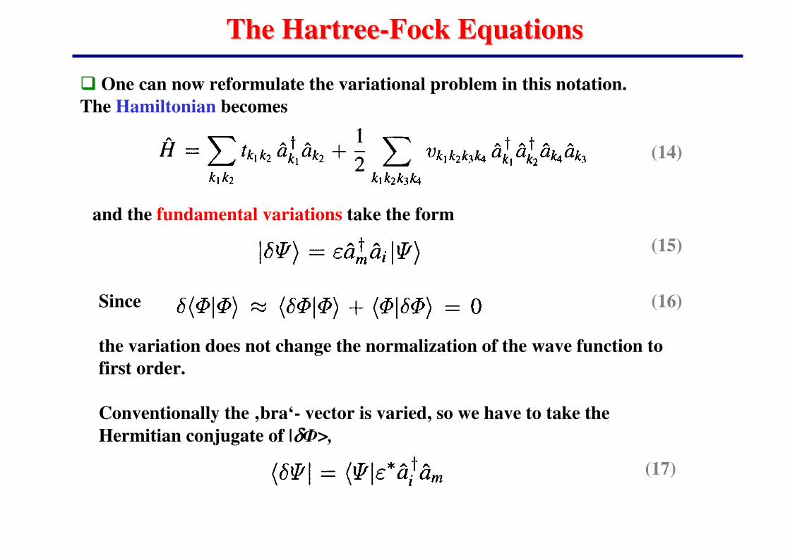
Since

the variation does not change the normalization of the wave function to

first order.

Conventionally the ‚bra‘- vector is varied, so we have to take the

Hermitian conjugate of |δδδδФ>,


(14)

� One can now reformulate the variational problem in this notation.

The Hamiltonian becomes

and the fundamental variations take the form

(15)

(16)

(17)


The variational equation now becomes

(18)

Insert (14) into (18) ….. ��

From the definition of the matrix elements follows that they do not change

their value if the first index is exchanged with the second and simultaneously

the third with the fourth ( ), so the equation can be simplified to

the matrix equation:

(19)

The notation is further simplified by abbreviating the antisymmetrized

matrix element as

(20)

(21)

Here i denotes an occupied state (i< A), m an unoccupied one (m > A), and j

sums over all occupied states.

The equation (22) requires that the single-particle states should be chosen such

that the matrix elements

vanish between occupied and unoccupied states.

If we allow (k,l) to refer to arbitrary combinations of states, this defines a single-

particle operator h in the Hilbert space, which is called the single-particle or

Hartree-Fock Hamiltonian.

The condition (22) characterizes the set of occupied states and not those states

individually.


We obtain (22)

(23)


(24)

Let‘s split the operator h h into four parts corresponding to different index ranges:

� hhрррр (particle-particle) denotes those matrix elements with both indices referring

to unoccupied single-particle states,

�� hhhhhh (hole-hole) has both states occupied,

�� hhphph and hhhhpp denote the appropriate mixed cases:

with the condition (22):

To fulfill these conditions: the states may be chosen such as to make hh itself

diagonal:

(25)

(25) - Hartree-Fock equations with single-particle energies εεεεk

The HartreeThe Hartree--Fock EquationFock Equation

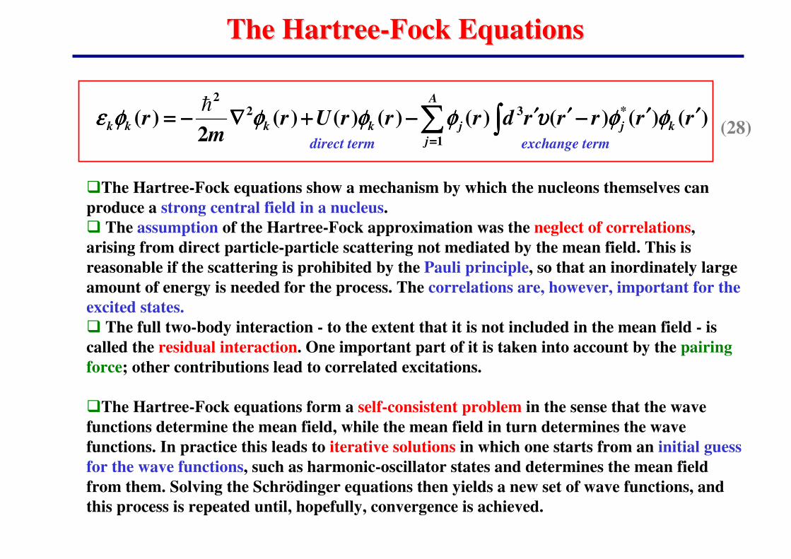
Writing the Hartree-Fock equations (25) in configuration space we get:

(26)

�The equations are quite similar in form to Schrödinger equations for each of

the single-particle states. The second term on the right-hand side is the

average potential(27)

which has the simple interpretation of the mean-field potential generated by

folding the interaction with the density distribution of nucleons.

�The last term is the exchange term; together with the average potential it defines

the mean field.

�The Hartree-Fock approximation is often called the mean-field approximation.

average potential

exchange term


�The Hartree-Fock equations show a mechanism by which the nucleons themselves can

produce a strong central field in a nucleus.

� The assumption of the Hartree-Fock approximation was the neglect of correlations,

arising from direct particle-particle scattering not mediated by the mean field. This is

reasonable if the scattering is prohibited by the Pauli principle, so that an inordinately large

amount of energy is needed for the process. The correlations are, however, important for the

excited states.

� The full two-body interaction - to the extent that it is not included in the mean field - is

called the residual interaction. One important part of it is taken into account by the pairing

force; other contributions lead to correlated excitations.

�The Hartree-Fock equations form a self-consistent problem in the sense that the wave

functions determine the mean field, while the mean field in turn determines the wave

functions. In practice this leads to iterative solutions in which one starts from an initial guess

for the wave functions, such as harmonic-oscillator states and determines the mean field

from them. Solving the Schrödinger equations then yields a new set of wave functions, and

this process is repeated until, hopefully, convergence is achieved.

)()()()()()()(2

)( *3

1

22

rrrrrdrrrUrm

r kj

A

j

jkkkk′′′′′′′′−−−−′′′′′′′′−−−−++++∇∇∇∇−−−−==== ∫∫∫∫∑∑∑∑

====

φφφφφφφφυυυυφφφφφφφφφφφφφφφφεεεεh

exchange termdirect term(28)

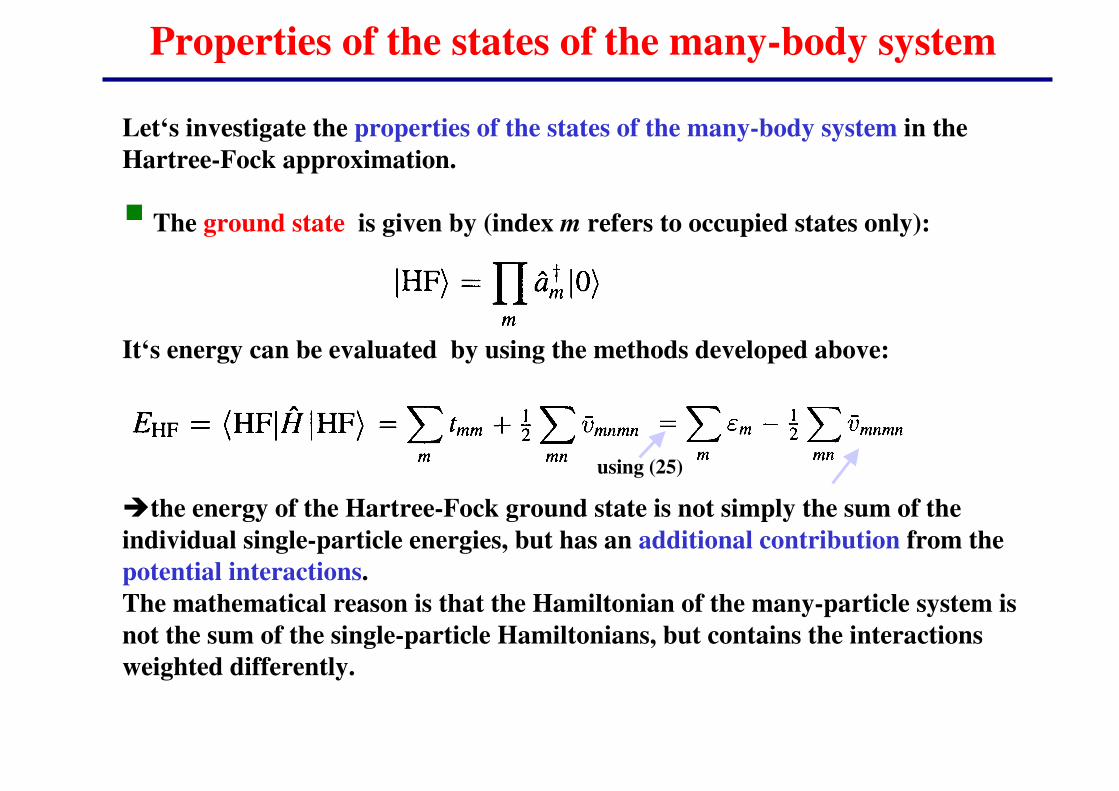
Properties of the states of the many-body system

Let‘s investigate the properties of the states of the many-body system in the

Hartree-Fock approximation.

� The ground state is given by (index m refers to occupied states only):

It‘s energy can be evaluated by using the methods developed above:

�the energy of the Hartree-Fock ground state is not simply the sum of the

individual single-particle energies, but has an additional contribution from the

potential interactions.

The mathematical reason is that the Hamiltonian of the many-particle system is

not the sum of the single-particle Hamiltonians, but contains the interactions

weighted differently.

using (25)


�Let‘s now construct excited states based on the Hartree-Fock ground state:

these should simply be given by the particle-hole excitations of various orders.

Construct excited states as one-particle/one-hole (1p1h) excitations :

or two-particle/two-hole (2p2h) excitations :

The expectation value of the energy of (1p1h) states:

Thus in addition to the expected contribution from the single-particle energies

of the two particles involved, there is also one arising from the change in the

mean field.

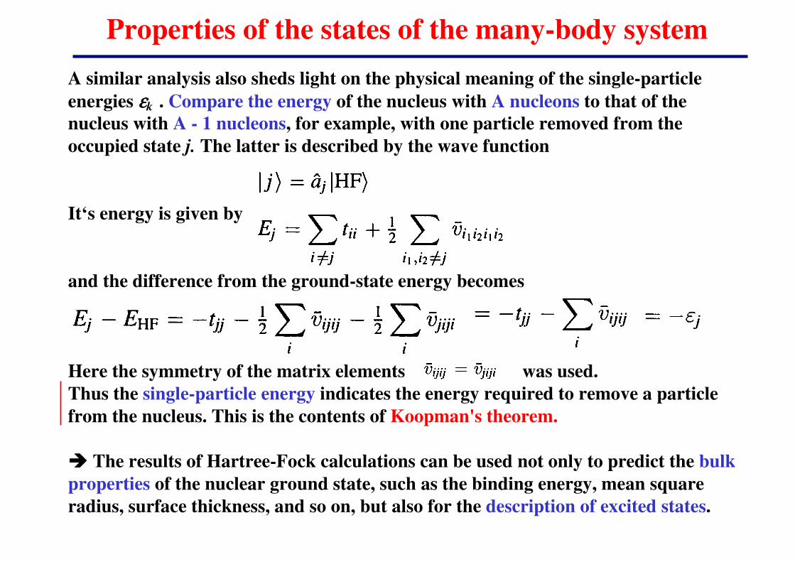
A similar analysis also sheds light on the physical meaning of the single-particle

energies εεεεk . Compare the energy of the nucleus with A nucleons to that of the

nucleus with A - 1 nucleons, for example, with one particle removed from the

occupied state j. The latter is described by the wave function

It‘s energy is given by

and the difference from the ground-state energy becomes

Here the symmetry of the matrix elements was used.

Thus the single-particle energy indicates the energy required to remove a particle

from the nucleus. This is the contents of Koopman's theorem.

�� The results of Hartree-Fock calculations can be used not only to predict the bulk

properties of the nuclear ground state, such as the binding energy, mean square

radius, surface thickness, and so on, but also for the description of excited states.


Hartree -Fock Theoryatlas.physics.arizona.edu/~shupe/Indep_Studies... · Hartree -Fock...

Documents

Transcript of Hartree -Fock Theoryatlas.physics.arizona.edu/~shupe/Indep_Studies... · Hartree -Fock...