131

NORTHWESTERN NATURALIST 86:131–143 WINTER 2005

HABITAT SELECTION MODELS FOR PACIFIC SANDLANCE (AMMODYTES HEXAPTERUS ) IN

PRINCE WILLIAM SOUND, ALASKA

WILLIAM D OSTRAND AND TRACEY A GOTTHARDT1

US Fish and Wildlife Service, Migratory Bird Management, 1011 E Tudor Road,Anchorage, Alaska 99503 USA: williampostrand@fws.gov

SHAY HOWLIN

Western EcoSystems Technology, Inc., 2003 Central Avenue,Cheyenne, Wyoming 82001 USA

MARTIN D ROBARDS2

Alaska Biological Science Center, Biological Resources Division, US Geological Survey,1011 E Tudor Road, Anchorage, Alaska 99503 USA

ABSTRACT—We modeled habitat selection by Pacific sand lance (Ammodytes hexapterus) by ex-amining their distribution in relation to water depth, distance to shore, bottom slope, bottomtype, distance from sand bottom, and shoreline type. Through both logistic regression and clas-sification tree models, we compared the characteristics of 29 known sand lance locations to 58randomly selected sites. The best models indicated a strong selection of shallow water by sandlance, with weaker association between sand lance distribution and beach shorelines, sand bot-toms, distance to shore, bottom slope, and distance to the nearest sand bottom. We applied aninformation-theoretic approach to the interpretation of the logistic regression analysis and de-termined importance values of 0.99, 0.54, 0.52, 0.44, 0.39, and 0.25 for depth, beach shorelines,sand bottom, distance to shore, gradual bottom slope, and distance to the nearest sand bottom,respectively. The classification tree model indicated that sand lance selected shallow-water hab-itats and remained near sand bottoms when located in habitats with depths between 40 and 60m. All sand lance locations were at depths ,60 m and 93% occurred at depths ,40 m. Probablereasons for the modeled relationships between the distribution of sand lance and the indepen-dent variables are discussed.

Key words: Ammodytes hexapterus, sand lance, habitat selection, logistic regression, classifi-cation tree models, Prince William Sound, Alaska.

Pacific sand lance (Ammodytes hexapterus)play an important ecological role as energy-rich prey (Anthony and Roby 1997) for sea-birds, marine mammals, and predatory fishesin Prince William Sound (PWS), Alaska (Kuletzand others 1997). Elsewhere, sand lance popu-lation dynamics have been correlated to the re-

1 Present address: Alaska Natural Heritage Program,Environment and Natural Resource Institute, Universityof Alaska Anchorage, 707 A Street, Anchorage, Alaska99501 USA.2 Present address: Resilience and Adaptation Program,Department of Biology and Wildlife, PO Box 756100,Fairbanks, Alaska 99775-6100 USA.

productive success of several seabirds, includ-ing great skuas (Catharacta skua), parasitic jae-gers (Stercorarius parasiticus), shags (Phalacro-corax aristotelis), black-legged kittiwakes (Rissatridactyla), Arctic terns (Sterna paradisaea), com-mon terns (Sterna hirundo), Atlantic puffins(Fratercula arctica), tufted puffins (Fratercula cir-rhata), and rhinoceros auklets (Cerorhinca mon-ocerata) (Willson and others 1999). In contrast toits importance in marine food webs, there hasbeen little quantification of ecological parame-ters that regulate distribution of this species(McGurk and Warburton 1992).

Pacific sand lance are commonly found inshallow, near-shore habitats where they bur-

132 NORTHWESTERN NATURALIST 86(3)

row in sandy substrates, avoiding rocky, mud-dy, and coarse gravel bottoms (Reay 1970). Byburrowing into substrates for refuge (while notforaging or during winter) sand lance effec-tively reduce their risk of predation and energyexpenditure (Pinto and others 1984). Sandlance burrow in both subtidal (Hobson 1986)and intertidal (Dick and Warner 1982) sub-strates and are associated with moderatelysloped beaches composed of well-washed grav-el or finer sands (Dick and Warner 1982).Wright and others (2000) also observed thatlesser sand eels (A. marinus) associate withsandy substrates and avoid those with .10%fine material. While not burrowed, Pacific sandlance generally remain close to sandy refuges(Kohlmann and Karst 1967; Hobson 1986).Kohlmann and Karst (1967) observed that sandeels (Ammodytes sp.) of the Baltic Sea forageddiurnally, moving farther offshore during day-light hours and returning to burrow in shallownearshore sand bottoms at night.

We infer from the apparent ecological im-portance of sand lance that resource managersand planners will find it useful to be able topredict important sand lance habits in order tomaintain productivity of nearshore ecosys-tems. The studies above present descriptive in-formation on habitat variables associated withsand lances (Ammodytes spp.). We have accept-ed that each of the variables presented aboveare important factors in sand lance habitat se-lection. We did not seek to find new habitat as-sociations; rather, our goals were to gain fur-ther understanding of the relative importanceof these variables and to demonstrate how theymight be used to model Pacific sand lance hab-itat selection.

METHODS

Study Area

We conducted this study in PWS, an embay-ment of about 10,000 km2 located on the south-central coast of Alaska. The climate is maritimewith a mean annual precipitation of approxi-mately 1.6 m and moderate air temperatures forthe subarctic. The coastline of PWS is rugged,with mountains #4000 m in elevation, numer-ous islands, fjords, and tidewater glaciers.Nearshore bathymetry is characterized by bothshallow water shelves and steeply sloping bot-toms.

Four study areas were selected in PWS: (1)the northern study area, which included ValdezArm and Port Valdez; (2) the central study area,which included waters near Naked and KnightIslands; (3) the southern study area, which in-cluded Icy and Jackpot Bays; and (4) the northshore of Montague Island (Fig. 1). These loca-tions were selected because seabird foragingstudies indicated that sand lance were presentwithin each area (Irons and others 1997; Suryanand others 2000).

Hydroacoustic Data Collection

Some habitat variables (depth, bottom slope,and bottom type) were determined through theanalysis of hydroacoustic data. Haldorson andothers (1997) conducted both nearshore andpelagic hydroacoustic and catch studies withinPWS. Sand lance were only detected nearshore,consistent with the observations of Raey (1970).Therefore, we chose to utilize the most exten-sive nearshore hydroacoustic data set, whichwas collected 17–27 July 1997 (Haldorson andothers 1997; Ostrand and others 2005). Thissurvey used a commercial purse seiner, the 18-m F/V Miss Kaylee, as a data-collection plat-form. Data were collected with a single beam120 kHz BioSonics DT4000 system with a 68beam angle. Transects were run at 11 kph withthe transducer towed beside the vessel. The ef-fective range of the equipment was 117 m fromthe transducer. Location data were obtainedfrom a precision lightweight global positioningreceiver (PLGR). PLGR units have a worst-casehorizontal position accuracy of 10 m at speeds,36 kph (Anonymous 1995).

Hydroacoustic Survey Design

The hydroacoustic study used 1- 3 12-kmshoreline blocks located within the 4 study ar-eas (Haldorson and others 1997; Ostrand andothers 2005). Prior to the survey, contiguousblocks were delineated in study areas, whichincluded all available shoreline. Due to thelarge extent of the northern and southern areasand the impracticality of sampling their entireshorelines, alternate blocks and 1 additionalrandomly selected block were deleted fromthese areas. All possible blocks were retainedin the central and Montague areas. The ulti-mate study design contained 9, 8, 8, and 2blocks in the north, central, south, and Monta-gue Island areas, respectively (see Table 1 for

WINTER 2005 133OSTRAND AND OTHERS: SAND LANCE HABITAT SELECTION

FIGURE 1. The 4 study areas, hydroacoustic transects, and sediment sample locations in Prince WilliamSound, Alaska.

134 NORTHWESTERN NATURALIST 86(3)

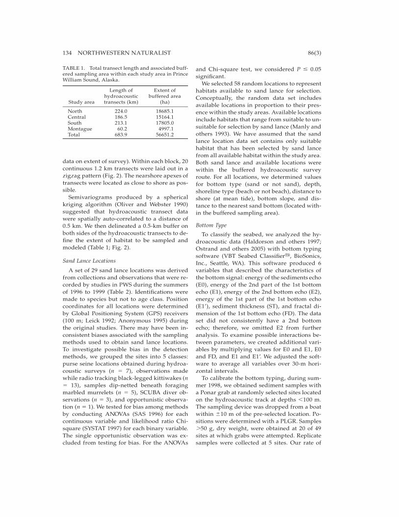
TABLE 1. Total transect length and associated buff-ered sampling area within each study area in PrinceWilliam Sound, Alaska.

Study area

Length ofhydroacoustictransects (km)

Extent ofbuffered area

(ha)

NorthCentralSouthMontagueTotal

224.0186.5213.160.2

683.9

18685.115164.117805.04997.1

56651.2

data on extent of survey). Within each block, 20continuous 1.2 km transects were laid out in azigzag pattern (Fig. 2). The nearshore apexes oftransects were located as close to shore as pos-sible.

Semivariograms produced by a sphericalkriging algorithm (Oliver and Webster 1990)suggested that hydroacoustic transect datawere spatially auto-correlated to a distance of0.5 km. We then delineated a 0.5-km buffer onboth sides of the hydroacoustic transects to de-fine the extent of habitat to be sampled andmodeled (Table 1; Fig. 2).

Sand Lance Locations

A set of 29 sand lance locations was derivedfrom collections and observations that were re-corded by studies in PWS during the summersof 1996 to 1999 (Table 2). Identifications weremade to species but not to age class. Positioncoordinates for all locations were determinedby Global Positioning System (GPS) receivers(100 m; Leick 1992; Anonymous 1995) duringthe original studies. There may have been in-consistent biases associated with the samplingmethods used to obtain sand lance locations.To investigate possible bias in the detectionmethods, we grouped the sites into 5 classes:purse seine locations obtained during hydroa-coustic surveys (n 5 7), observations madewhile radio tracking black-legged kittiwakes (n5 13), samples dip-netted beneath foragingmarbled murrelets (n 5 5), SCUBA diver ob-servations (n 5 3), and opportunistic observa-tion (n 5 1). We tested for bias among methodsby conducting ANOVAs (SAS 1996) for eachcontinuous variable and likelihood ratio Chi-square (SYSTAT 1997) for each binary variable.The single opportunistic observation was ex-cluded from testing for bias. For the ANOVAs

and Chi-square test, we considered P # 0.05significant.

We selected 58 random locations to representhabitats available to sand lance for selection.Conceptually, the random data set includesavailable locations in proportion to their pres-ence within the study areas. Available locationsinclude habitats that range from suitable to un-suitable for selection by sand lance (Manly andothers 1993). We have assumed that the sandlance location data set contains only suitablehabitat that has been selected by sand lancefrom all available habitat within the study area.Both sand lance and available locations werewithin the buffered hydroacoustic surveyroute. For all locations, we determined valuesfor bottom type (sand or not sand), depth,shoreline type (beach or not beach), distance toshore (at mean tide), bottom slope, and dis-tance to the nearest sand bottom (located with-in the buffered sampling area).

Bottom Type

To classify the seabed, we analyzed the hy-droacoustic data (Haldorson and others 1997;Ostrand and others 2005) with bottom typingsoftware (VBT Seabed Classifiery, BioSonics,Inc., Seattle, WA). This software produced 6variables that described the characteristics ofthe bottom signal: energy of the sediments echo(E0), energy of the 2nd part of the 1st bottomecho (E1), energy of the 2nd bottom echo (E2),energy of the 1st part of the 1st bottom echo(E1’), sediment thickness (ST), and fractal di-mension of the 1st bottom echo (FD). The dataset did not consistently have a 2nd bottomecho; therefore, we omitted E2 from furtheranalysis. To examine possible interactions be-tween parameters, we created additional vari-ables by multiplying values for E0 and E1, E0and FD, and E1 and E1’. We adjusted the soft-ware to average all variables over 30-m hori-zontal intervals.

To calibrate the bottom typing, during sum-mer 1998, we obtained sediment samples witha Ponar grab at randomly selected sites locatedon the hydroacoustic track at depths ,100 m.The sampling device was dropped from a boatwithin 610 m of the pre-selected location. Po-sitions were determined with a PLGR. Samples.50 g, dry weight, were obtained at 20 of 49sites at which grabs were attempted. Replicatesamples were collected at 5 sites. Our rate of

WINTER 2005 135OSTRAND AND OTHERS: SAND LANCE HABITAT SELECTION

FIGURE 2. Paired maps of the 4 study areas depicting Pacific sand lance (Ammodytes hexapterus) and randomlocations, hydroacoustic transects with 0.5-km buffer, sand bottoms, beach and non-beach shorelines, andwater depth.

sampling success indicated to us that the Ponargrab was not of sufficient size to consistentlysample the bottom within PWS. To improvesampling success rate we changed gear the fol-lowing year. During the summer of 1999, wecollected samples from 28 of 30 sites with a Shi-pek bottom grab. Duplicate samples were col-lected at 23 of these sites. We also collected 21samples from 24 sites with a bottom dredgewith a 28 3 76-cm opening and 76-cm depth,

during July 1999. One sample was collected ateach dredge site. The final bottom typing vali-dation data set contained 69 samples (Fig. 1).

Sediment samples were frozen and then ovendried (1508 C for 3 h) prior to laboratory anal-ysis. Grain size analysis was performed on sed-iment samples using a sieve procedure (Day1965), which determined percentage gravel,sand, silt, and clay for each sample followingthe USDA scale (Gee and Bauder 1986). For

136N

OR

TH

WE

STE

RN

NA

TU

RA

LIST

86(3)

TABLE 2. Sand lance locations used in developing habitat selection models for Prince William Sound, Alaska.

Year No. of locations MethodMaximum Depth

for Year and Method Reference

1996 2 Visually observed by SCUBA divers. 0 Dean and others 20001 Purse seined schools located by hydroacoustic sur-

vey.10 Haldorson and others 1997

1997 1 Visually observed by SCUBA divers. 35 Dean and others 19996 Purse seined schools located by hydroacoustic sur-

vey.39 Haldorson and others 1998

1 Visually observed fish caught by radio trackedblack-legged kittiwakes.

4 *DB Irons

1998 4 Visually observed fish caught by radio racked black-legged kittiwakes.

39 *DB Irons

2 Dip netted schools foraged on by radio trackedblack-legged kittiwakes.

52 Suryan and others 2000

1999 6 Dip netted schools foraged on by radio rackedblack-legged kittiwakes.

36 Suryan and others 2000

5 Dip netted schools foraged on by marbled murreletsobserved during systematic surveys.

49 Kuletz 1999

1 Visually observed during black-legged kittiwake col-ony survey.

22 *DB Irons

* Unpublished data. DB Irons, US Fish and Wildlife Service, Migratory Bird Management, 1011 E Tudor Road, Anchorage, Alaska 99503.

WINTER 2005 137OSTRAND AND OTHERS: SAND LANCE HABITAT SELECTION

sites where 2 samples were taken, they wereanalyzed separately and the results were av-eraged. Samples were designated as sand,$80% sand, or not sand (Folk 1980).

To ascribe the bottom types throughout ourstudy areas we used S-plus (MathSoft 1999)classification tree modeling (Chambers andHastie 1992; Bell 1996). We used the 69 sedi-ment classifications of the validation data as thedependent variable and the associated values ofthe characteristics of the hydroacoustic bottomsignals as independent variables for the train-ing data set. Trees were overfit to the data, set-ting S-plus options of minimum deviance 5 0and minimum size 5 2. Model selection andmisclassification rate estimation were based ona jackknife procedure. Initially we removed the1st observation from the data set and fit the treeto the remaining observations. The number ofterminal nodes (size) of the tree was reduced(pruned) to each size between 1 and the un-pruned tree size, and the 1st observation wasclassified by each of these trees. The pruningfunction uses cost-complexity to determine theoptimal tree of a specified size (Chambers andHastie 1992; Bell 1996). We noted if the classi-fications of the 1st observation were correct.Next, we replaced the 1st observation and re-moved the 2nd observation and repeated thepruning and classification procedures. Thismethod was continued until each observationhad been removed from the data set and re-classified by trees of each size. The %-misclas-sification rate (the number of incorrect classi-fications divided by the number of observations3 100) was calculated for each tree. We selectedthe tree size having the lowest jackknifed mis-classification error rate to predict the bottomtype of the sampling areas. We considered mis-classification rates .25% to be unacceptable.

Depth, Bottom Slope, Distance to Shore, andDistance to the Nearest Sand

The bathymetry within the sampling areawas determined by kriging (Oliver and Webster1990) depth values extracted from the hydroa-coustic data set. The maximum depth recordedby hydroacoustics was 117 m. All locationswithin the sampling area deeper than 117 mwere excluded from analysis. Sand lance aremost commonly found in shallow water (,50m) and rarely occur at depths of .100 m (Ro-bards and Piatt 1999) justifying this demarca-

tion. To account for the slope from shore, ad-jacent coastline depths were made equal to 0and incorporated in the kriging. A slope cov-erage, expressed in degrees (0 to 908), was cal-culated within ARC/INFOy from depth andlocation data coverages. Distance to shore anddistance to the nearest sand bottom valueswere determined for sand lance and random lo-cations using ARC/INFOy.

Shoreline Type

Shoreline habitat type was determinedthrough aerial visual observations conductedduring spring 1999. These data were digitizedand converted into a GIS coverage (ResearchPlanning Inc., PO Box 328, 1121 Park Street,Columbia, SC, unpubl. data). Shorelines wereclassified as exposed rocky shores, exposedsolid man-made structures, exposed wave-cutplatforms in bedrock, fine- to medium-grainedsand beaches, mixed sand and gravel beaches,gravel beaches, riprap, exposed tidal flats, shel-tered rocky shores, sheltered riprap, vegetatedsteeply-sloping bluffs, sheltered tidal flats, andsalt- and brackish-water marshes. We conduct-ed a preliminary analysis with the 2 modelingmethods (see modeling techniques below) andfound no relation between shoreline class anddistribution of sand lance. The beach shorelinetypes (fine- to medium-grained sand beaches,mixed sand and gravel beaches, and gravelbeaches) were descriptively similar to the in-tertidal habitats that Dick and Warner (1982)and Robards and Piatt (MD Robards and JFPiatt, Biological Research Division, US Geolog-ical Survey, 1011 E. Tudor Road, Anchorage,AK, unpubl. data) observed to be sand lancehabitat in areas near PWS. Therefore, we col-lapsed shoreline types into beaches and non-beaches for final analyses.

Habitat Selection Models

We applied both logistic regression (Manlyand others 1993; SAS 1996) and classificationtree (Chambers and Hastie 1992; Bell 1996;MathSoft 1999) methods to model sand lancehabitat selection. Because these methods ex-amine data differently and may produce dif-ferent results (Dettmers and others 2002), wechose to use both methods to obtain a broadprospective on habitat selection. For both meth-ods, we compared the characteristics of knownsand lance locations to available (random) lo-

138 NORTHWESTERN NATURALIST 86(3)

TABLE 3. The 15 logistic regression models of habitat selection by sand lance for which the corrected Akai-ke’s information criterion (AICc) value was within 2 of the lowest value observed. The P for all models pre-sented 5 0.0001.

Model AICc D AICca

Habb 5 2.08 2 0.04Depc 1 1.20Sand 1 1.11Beae

Hab 5 20.24 2 0.04Dep 1 1.13BeaHab 5 3.01 2 0.04Dep 2 1.19SanHab 5 2.32 2 0.04Dep 1 1.27Bea 1 1.27San 2 0.007Distf

Hab 5 0.74 2 0.042Dep

95.2295.4593.8295.8895.92

0.000.230.520.660.70

Hab 5 20.14 2 0.03Dep 1 1.29Bea 2 0.0007DistHab 5 1.40 2 0.03Dep 2 0.0009Dist 2 0.10Slopg

Hab 5 0.43 2 0.03Dep 2 0.001Dist 1 1.12Bea 2 0.09SlopHab 5 0.95 2 0.04Dep 2 0.06SlopHab 5 3.28 2 0.04Dep 1 1.24San 2 0.0005Dist

96.2196.5596.6196.7596.77

0.991.331.391.531.55

Hab 5 2.57 2 0.03Dep 2 0.001Dist 1 1.15Bea 1 1.15San 2 0.08SlopHab 5 3.40 2 0.03Dep 2 0.0009Dist 1 1.07San 2 0.09SlopHab 5 2.96 2 0.04Dep 1 1.07San 2 0.05SlopHab 5 0.03 2 0.04Dep 1 1.01Bea 2 0.05SlopHab 5 2.08 2 0.04Dep 1 1.11Bea 1 1.20San 2 0.004Slop

96.8196.8596.9297.0497.16

1.591.631.691.821.94

a The difference of model AICc from the lowest value observed.b Type of habitat, either suitable or not suitable for sand lance.c Depth of water.d Sand Bottom.e Beach Shoreline.f Distance to Shore.g Slope of the Bottom.

cations. Presence of sand lance or available lo-cation was the dependent variable; bottomtype, depth, distance to shore, bottom slope,distance to the nearest sand, and shoreline typewere the independent variables. Presence ofsand lance or available location, bottom type,and shoreline type data were binary and allother variables were continuous.

Prior to conducting regressions, variableswere checked for independence through cor-relation analysis (SAS 1996). We considered r ,0.50 to indicate independence. We then devel-oped a model set composed of all possible com-binations of 6 variables excluding interactionsand higher order terms (63 models). Logisticregression was fitted to all equations within themodel set, and these were ranked based uponAkaike’s information criterion corrected forsmall sample sizes (AICc) (Akaike 1973; Burn-ham and Anderson 1998). The AICc statistic de-scribes the fit of a model while penalizing forvariables that explain minimal error. Burnhamand Anderson (1998) have suggested that allmodels whose AICc values differ from the low-est observed AICc by ,2 (difference from low-est AICc, hereafter D AICc) should receive con-sideration. We examined all models that had DAICc ,2 and made descriptive comparisons ofthem. We also determined importance values(Burnham and Anderson 1998) from the set of

all possible models for each independent vari-able using the candidate model set. Importancevalues are the sum of Akaike weights of themodels in which the variable is included. Clas-sification tree model selection followed thesame procedures as presented under bottomtyping.

RESULTS

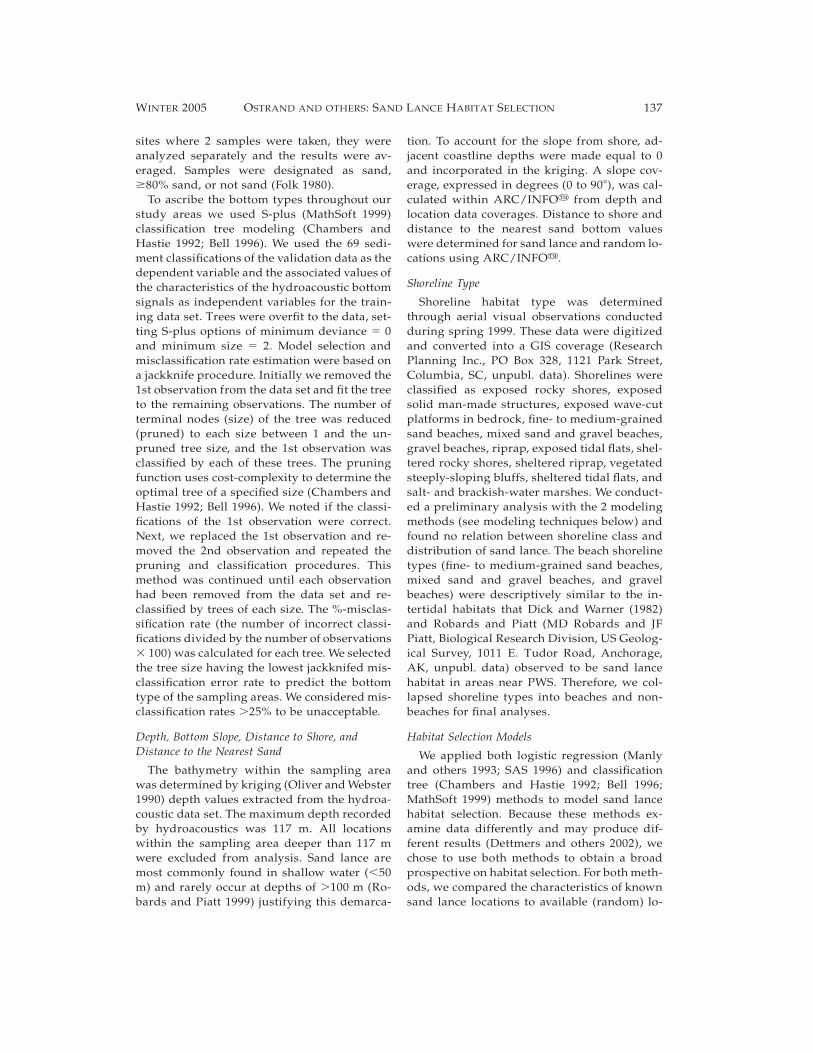
The logistic regression and classification treemodels all indicated a strong association be-tween sand lance distribution and depth, withweaker and inconsistent relationships to beachshorelines, bottom type, distance to shore, bot-tom slope, and distance to the nearest sand bot-tom (Table 3, Fig. 3). Fifteen logistic regressionmodels had D AICc ,2 and all of these werehighly significant (P 5 0.0001; Table 3). All ofthese models contained depth as a variable,with an individual variable P , 0.05. No othervariable appeared in all 15 models. Distance tothe nearest sand bottom was the only variablethat did not appear in any of the 15 models. Theimportance values of the independent vari-ables, out of a maximum value of 1.00, weredepth 5 0.99, shoreline type 5 0.54, bottomtype 5 0.52, distance to shore 5 0.44, slope ofthe bottom 5 0.39, and distance to the nearestsand bottom 5 0.25. The classification treemodel had a jackknife misclassification of 10%.

WINTER 2005 139OSTRAND AND OTHERS: SAND LANCE HABITAT SELECTION

FIGURE 3. Best classification tree model of habitatselection by Pacific sand lance (Ammodytes hexapte-rus). The variables included in the model are depthof water (m) and distance from the nearest sand bot-tom (m). At each node, data that are less than the de-picted value are split left and data greater than thevalue continue down the branching to the right. Atthe terminal nodes, 1 designates suitable and 2 in-dicates unsuitable habitat and the value is the nodesample size.

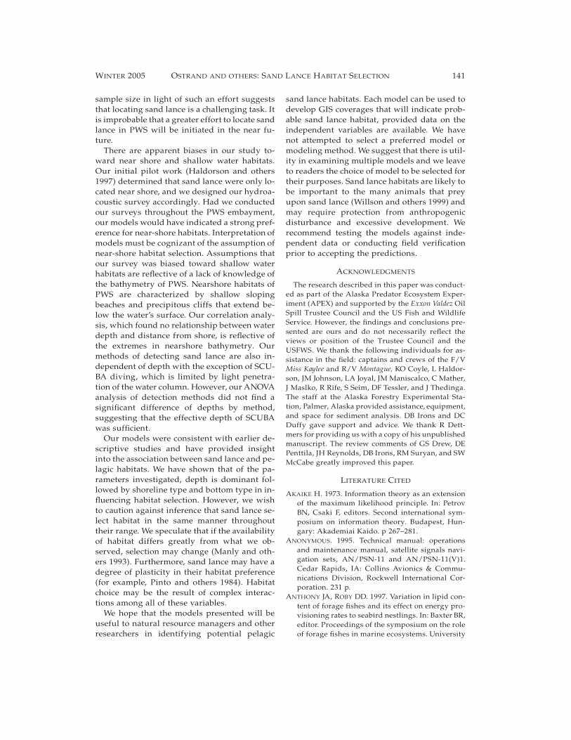
FIGURE 4. Paired histograms showing the distri-butions of data on depth, distance to shore, bottomslope, and distance to the nearest sand bottom for Pa-cific sand lance (Ammodytes hexapterus) and randomlocations. Data on shoreline and bottom type werebinary and are not depicted.

The tree indicated that at depth .40 m, habitatselection was based upon distance-to-sand anddepth. We further examined the distance-to-sand variable at depths .40 m and determinedthat x 5 37.7, s 5 53.3 m, n 5 2 for sand lancelocations, and x 5 610.9, s 5 741.5 m, n 5 36for available sites.

Values (x 6 s) for continuous variables at lo-cations where sand lance were present and atavailable locations were 21.1 6 16.7 and 53.1 636.3 m depth; 418.3 6 377.3 and 688.4 6 584.2m distance from shore; 3.6 6 2.9 and 5.7 6 6.2degrees slope; 528.0 6 567.6 and 590 6 735.3 mdistance from the nearest sand bottom, respec-tively (see Fig. 4 for comparative histograms).Sand bottoms were associated with 20.7% (6) ofthe sand lance locations and 8.6% (5) of theavailable locations. Beach was the nearestshoreline type at 90.0% (26) and 69.0% (40) ofthe sand lance and available locations, respec-tively. We further examined our data to deter-mine if there was a relationship between beach(a binary variable) and bottom slope. At avail-able locations, bottom slopes associated withbeach shorelines (x 5 4.2, s 5 4.8, n 5 40) wereless steep than slopes associated with non-beach shorelines (x 5 9.2, s 5 7.7, n 5 18; Krus-kal Wallis 1-way ANOVA, H 5 5.28, P 5 0.022).All comparisons of the methods of collectingsand lance locations yielded non-significant re-sults (ANOVA test for depth P 5 0.81, slope P5 0.77, distance to the nearest sand bottom P5 0.60, and distance to shore P 5 0.09; likeli-hood ratio Chi-square tests for sand or not-sand bottom P 5 0.20 and for beach or not-beach shoreline P 5 0.67). Correlation analysisindicated that all possible pairs of variables hadr , 0.50, thereby meeting our requirements forindependence for all modeling components.

The bottom typing classification tree hadseven 7 nodes and utilized the following vari-ables: energy of the 1st part of the 1st bottomecho (E1’), energy of the 2nd part of the 1st bot-tom echo (E1), fractal dimension (FD), energyof the sediments echo (E0) 3 FD, and E1 3 E1’.The jackknife estimated misclassification ratewas 6%. We also attempted to model more than2 bottom types; however, these attempts re-sulted in unacceptable misclassification rates.

DISCUSSION

The models presented indicated that sandlance distribution was strongly associated with

140 NORTHWESTERN NATURALIST 86(3)

shallow water depths. Few of the sand lance lo-cations were at depths .40 m and none atdepths .60 m (Fig. 4), agreeing with previousestimates of sand lance depth distribution (Ro-bards and Piatt 1999). Selection for shallow wa-ter is consistent with the findings of Winslade(1974) that sand lance are visual foragers andare sensitive to light while burrowed. Hence,the limit of light penetration through the watercolumn may be the mechanism behind the se-lection of shallow habitats.

The importance values for the substrate var-iables shoreline type and bottom type ranked2nd and 3rd. These model outcomes indicateselection for beach shorelines over non-beachesand sand bottoms over other bottom types. Thelinkage between sand lance and sand sub-strates as burrowing habitat and refuge is welldocumented (Dick and Warner 1982; Hobson1986), and we had expected a strong associa-tion between sand lance distribution and theseparameters.

The importance values indicated that the as-sociation between sand lance distribution anddistance to shore and bottom slope ranked be-low depth and the substrate variables. A rela-tionship between distribution and distance toshore intuitively follows from the strong selec-tion for shallow habitat. Shallower water is ex-pected closer to shore; however, our correlationanalysis indicated that there was not a corre-spondence between depth and distance toshore. Within PWS, at the spatial scale of thisstudy, shallow water was available both close toand distant from shore, which may explain theimportance ranking of the variables. Our ex-amination of bottom slope relative to depthsuggests that moderate bottom slopes are as-sociated with beach habitats in PWS. Therefore,the inclusion of bottom slopes within logisticregression models having D AICc values ,2may be the result of covariance with beachshorelines.

The classification tree analyses yielded amodel with lower misclassification rate for bot-tom type than for habitat selection. This mayhave been a partial result of the nature of thedata sets examined in each analysis. Bottomtyping compared characteristics of known sandlocations to non-sand sites; whereas, the habi-tat selection model compared known sandlance locations to available, or random, sites.The presence of suitable sites within the avail-

able data set may have resulted in overfitting(Bell 1996; Burnham and Anderson 1998) as thetree modeling process attempted to classify thesuitable available sites as non-sand-lance loca-tions. In examining the habitat selection tree(Fig. 3), the data are 1st split at 40-m depth. Atdepths ,40 m are 5 terminal nodes, 1 of whichconferred a non-sand-lance habitat type. Thisnode indicated that if depth was 13 to 33 m andthe distance to the nearest sand bottom was 69to 560 m then the habitat was unsuitable forsand lance. To us, this branching was counter-intuitive and appeared to be the result of thetree accommodating available locations thatwere suitable for sand lance, indicating overfit-ting. The presented tree was determinedthrough a rigorous and objective jackknife pro-cedure; however, in light of the above argu-ments we suggest a modified model that indi-cates that habitat selection is based solely upondepth when depth is ,40 m. The resultingchange would be represented by a reduction to1 terminal node on the left side of the tree, be-low the initial split of the data at 40-m depth.

The habitat selection tree indicated that atdepth .40 m sand lance did not venture farfrom sand bottoms, consistent with the obser-vations of Hobson (1986). This relationship wasnot reported by logistic regression. The recur-sive partitioning of the data by the classifica-tion model (Chambers and Hastie 1992; Bell1996) has revealed a pattern in the data thatwould have otherwise remained undetectedand illustrates the value of multiple statisticalapproaches. However, we must caution againstthe over interpretation of this result due to thesmall number (n 5 2) of sand lance locationsobserved at depth .40 m. We suggest that thisis an interesting result worthy of further study.

The comparison of methods used to deter-mine sand lance locations failed to detect biasesin sampling methods. This finding substanti-ated our application of these data to developthe presented models. This was not a definitivecomparison of data collection methods, and wecaution against making further inferences fromthese results. The total sample size of verifiedsand lance locations was less than desirable tomake inference to an area as large as PWS.However, these data were collected by 5 differ-ent studies over 4 y. Each of the studies had aninterest in locating sand lance and put an em-phasis on recording their locations. The low

WINTER 2005 141OSTRAND AND OTHERS: SAND LANCE HABITAT SELECTION

sample size in light of such an effort suggeststhat locating sand lance is a challenging task. Itis improbable that a greater effort to locate sandlance in PWS will be initiated in the near fu-ture.

There are apparent biases in our study to-ward near shore and shallow water habitats.Our initial pilot work (Haldorson and others1997) determined that sand lance were only lo-cated near shore, and we designed our hydroa-coustic survey accordingly. Had we conductedour surveys throughout the PWS embayment,our models would have indicated a strong pref-erence for near-shore habitats. Interpretation ofmodels must be cognizant of the assumption ofnear-shore habitat selection. Assumptions thatour survey was biased toward shallow waterhabitats are reflective of a lack of knowledge ofthe bathymetry of PWS. Nearshore habitats ofPWS are characterized by shallow slopingbeaches and precipitous cliffs that extend be-low the water’s surface. Our correlation analy-sis, which found no relationship between waterdepth and distance from shore, is reflective ofthe extremes in nearshore bathymetry. Ourmethods of detecting sand lance are also in-dependent of depth with the exception of SCU-BA diving, which is limited by light penetra-tion of the water column. However, our ANOVAanalysis of detection methods did not find asignificant difference of depths by method,suggesting that the effective depth of SCUBAwas sufficient.

Our models were consistent with earlier de-scriptive studies and have provided insightinto the association between sand lance and pe-lagic habitats. We have shown that of the pa-rameters investigated, depth is dominant fol-lowed by shoreline type and bottom type in in-fluencing habitat selection. However, we wishto caution against inference that sand lance se-lect habitat in the same manner throughouttheir range. We speculate that if the availabilityof habitat differs greatly from what we ob-served, selection may change (Manly and oth-ers 1993). Furthermore, sand lance may have adegree of plasticity in their habitat preference(for example, Pinto and others 1984). Habitatchoice may be the result of complex interac-tions among all of these variables.

We hope that the models presented will beuseful to natural resource managers and otherresearchers in identifying potential pelagic

sand lance habitats. Each model can be used todevelop GIS coverages that will indicate prob-able sand lance habitat, provided data on theindependent variables are available. We havenot attempted to select a preferred model ormodeling method. We suggest that there is util-ity in examining multiple models and we leaveto readers the choice of model to be selected fortheir purposes. Sand lance habitats are likely tobe important to the many animals that preyupon sand lance (Willson and others 1999) andmay require protection from anthropogenicdisturbance and excessive development. Werecommend testing the models against inde-pendent data or conducting field verificationprior to accepting the predictions.

ACKNOWLEDGMENTS

The research described in this paper was conduct-ed as part of the Alaska Predator Ecosystem Exper-iment (APEX) and supported by the Exxon Valdez OilSpill Trustee Council and the US Fish and WildlifeService. However, the findings and conclusions pre-sented are ours and do not necessarily reflect theviews or position of the Trustee Council and theUSFWS. We thank the following individuals for as-sistance in the field: captains and crews of the F/VMiss Kaylee and R/V Montague, KO Coyle, L Haldor-son, JM Johnson, LA Joyal, JM Maniscalco, C Mather,J Maslko, R Rife, S Seim, DF Tessler, and J Thedinga.The staff at the Alaska Forestry Experimental Sta-tion, Palmer, Alaska provided assistance, equipment,and space for sediment analysis. DB Irons and DCDuffy gave support and advice. We thank R Dett-mers for providing us with a copy of his unpublishedmanuscript. The review comments of GS Drew, DEPenttila, JH Reynolds, DB Irons, RM Suryan, and SWMcCabe greatly improved this paper.

LITERATURE CITED

AKAIKE H. 1973. Information theory as an extensionof the maximum likelihood principle. In: PetrovBN, Csaki F, editors. Second international sym-posium on information theory. Budapest, Hun-gary: Akademiai Kaido. p 267–281.

ANONYMOUS. 1995. Technical manual: operationsand maintenance manual, satellite signals navi-gation sets, AN/PSN-11 and AN/PSN-11(V)1.Cedar Rapids, IA: Collins Avionics & Commu-nications Division, Rockwell International Cor-poration. 231 p.

ANTHONY JA, ROBY DD. 1997. Variation in lipid con-tent of forage fishes and its effect on energy pro-visioning rates to seabird nestlings. In: Baxter BR,editor. Proceedings of the symposium on the roleof forage fishes in marine ecosystems. University

142 NORTHWESTERN NATURALIST 86(3)

of Alaska Fairbanks, AK: Alaska Sea Grant Col-lege Program AK-SG-97–01. p 725–729.

BELL JF. 1996. Application of classification trees to thehabitat preference of upland birds. Journal of Ap-plied Statistics 23:349–359.

BURNHAM KP, ANDERSON DR. 1998. Model selectionand inference, a practical information-theoreticapproach. New York, NY: Springer-Verlag. 320 p.

CHAMBERS JM, HASTIE TJ. 1992. Statistical models inS. Pacific Grove, CA: Wadsworth & Brooks/ColeAdvanced Books & Software. 608 p.

DAY PR. 1965. Particle fractionation and particle-sizeanalysis, hydrometer method. In: Black CA, edi-tor. Methods of soil analysis, part I, AgronomyMonograph no. 9. Madison, WI: American Soci-ety of Agronomy-Soil Science Society of America.p 562–566.

DEAN TA, HALDORSON L, LAUR DR, JEWETT SC,BLANCHARD A. 2000. The distribution of near-shore fishes in kelp and eelgrass communities inPrince William Sound, Alaska: associations withvegetation and physical habitat characteristics.Journal of Environmental Biology of Fishes 57:271–287.

DETTMERS R, BUEHLER DA, BARTLETT JB. 2002. A testand comparison of wildlife-habitat modelingtechniques for predicting bird occurrence at a re-gional scale. In: Scott JM, Heglund PJ, MorrisonML, Haufler JB, Raphael MG, Wall WA, SamsonFB, editors. Predicting species occurrences: is-sues of accuracy and scale. Covelo, CA: IslandPress. p 607–616.

DICK MH, WARNER IM. 1982. Pacific sand lance, Am-modytes hexapterus Pallas, in the Kodiak Islandgroup, Alaska. Syesis 15:43–50.

FOLK FL. 1980. Petrology of sedimentary rocks. Aus-tin, TX: Hemphill Publishing Co. 182 p.

GEE GW, BAUDER JW. 1986. Particle-size analysis. In:Klute A, editor. Methods of Soil Analysis, Part I.Physical and mineralogical methods-agronomymonograph no. 9. Madison, WI: American Societyof Agronomy-Soil Science Society of America. p338–411.

*HALDORSON L, SHIRLEY T, COYLE KO, THORNE R.1997. Forage species studies in Prince WilliamSound, project 163a annual report. In: Duffy DC,compiler. APEX project: Alaska Predator ecosys-tem experiment in Prince William Sound and theGulf of Alaska, Exxon Valdez oil spill restorationproject annual report (restoration project 96163),Appendix A. Anchorage, AK: Alaska Natural

* Unpublished. Available from: Alaska Resources Li-brary and Information Services, Room 111, LibraryBuilding, 3211 Providence Drive, Anchorage, AK99508.

Heritage Program and Department of Biology,University of Alaska Anchorage. 93 p.

*HALDORSON L, SHIRLEY T, COYLE KO, AND THORNE

R. 1998. Forage species studies in Prince WilliamSound, restoration project 97163a annual report.In: Duffy DC, compiler. APEX project: Alaskapredator ecosystem experiment in Prince WilliamSound and the Gulf of Alaska, Exxon Valdez oilspill restoration project annual report (restora-tion project 97163), appendix A. Anchorage, AK:Alaska Natural Heritage Program and Depart-ment of Biology, University of Alaska Anchorage.10 p.

HOBSON ES. 1986. Predation of the Pacific sand lance,Ammodytes hexapterus (Pisces: Ammodytidae),during the transition between day and night insoutheastern Alaska. Copeia 1986:223–226.

*IRONS DB, SURYAN RM, BENSON J. 1997. Kittiwakesas indicators of forage fish availability. In: DuffyDC, compiler. APEX project: Alaska predator eco-system experiment in Prince William Sound andthe Gulf of Alaska, Exxon Valdez oil spill restora-tion project annual report (restoration project96163), appendix E. Anchorage, AK: Alaska Nat-ural Heritage Program and Department of Biol-ogy, University of Alaska Anchorage. 19 p.

KOHLMANN DHH, KARST H. 1967. Freiwasserbeo-bachtungen zum Verhalten von Toviasfischsch-warmen (Ammodytidae) in der westlichen Os-tsee. Zeitschrift fur Tierpsychologie 24:282–297.

*KULETZ, KJ. 1999. Marbled murrelet productivityrelative to forage fish abundance and chick diet.In: Duffy DC, compiler. APEX project: Alaskapredator ecosystem experiment in Prince WilliamSound and the Gulf of Alaska, Exxon Valdez oilspill restoration project annual report (restora-tion project 96163), appendix R. Kaulua, HI: Pau-manok Solutions. p 348–381.

KULETZ KJ, IRONS DB, AGLER BA, PIATT JF, DUFFY DC.1997. Long-term changes in diets and popula-tions of piscivorous birds and mammals in PrinceWilliam Sound, Alaska. In: Baxter BR, editor. Pro-ceedings of the symposium on the role of foragefishes in marine ecosystems. Fairbanks, AK: Alas-ka Sea Grant College Program AK-SG-97-01, Uni-versity of Alaska Fairbanks. p 703–706.

LEICK A. 1992. Introducing GPS surveying tech-niques. ACSM Bulletin 138:47–48.

MANLY BFJ, MCDONALD LL, THOMAS DL. 1993. Re-source selection by animals, statistical designanalysis for field studies. London, UK: Chapmanand Hall. 177 p.

MATHSOFT. 1999. S-Plus 2000 guide to statistics, vol.1. Seattle, WA: MathSoft, Inc. 638 p.

MCGURK MD, WARBURTON HD. 1992. Pacific sandlance of the Port Moller estuary, southeastern Be-ring Sea: an estuarine-dependent early life his-tory. Fisheries Oceanography 1:306–320.

WINTER 2005 143OSTRAND AND OTHERS: SAND LANCE HABITAT SELECTION

OLIVER MA, WEBSTER R. 1990. Kriging: a method ofinterpolation for geographical information sys-tems. International Journal of Geographical In-formation Systems 4:313–332.

OSTRAND WD, HOWLIN S, GOTTHARDT TA. 2005. Fishschool selection by marbled murrelets in PrinceWilliam Sound Alaska: responses to changes inavailability. Marine Ornithology. In press.

PINTO JM, PEARSON WH, ANDERSON JW. 1984. Sedi-ment preferences and oil contamination in the Pa-cific sand lance Ammodytes hexapterus. Marine Bi-ology 83:193–204.

REAY PJ. 1970. Synopsis of biological data on NorthAtlantic sandeels of the genus Ammodytes. FAOFisheries Synopsis No. 82. Rome, Italy: Food andAgriculture Organization of the United Nations.48 p.

*ROBARDS MD, PIATT JF. 1999. Biology of the genusAmmodytes, the sand lances. In: Robards MD,Willson MF, Armstrong RH, Piatt JF, editors. Sandlance: a review of biology and predator relationsand annotated bibliography. Research PaperPNW-RP-521. Portland, OR: USDA Forest Service,Pacific Northwest Research Station. p 1–6.

SAS. 1996. SAS/STAT User’s Guide: Volume 1, Ver-sion 6, 4th ed. Cary, NC: SAS Institute, Inc. 943 p.

SURYAN RM, IRONS DB, BENSON J. 2000. Prey switch-ing and variable foraging strategies of black-leg-ged kittiwakes and the effect on reproductivesuccess. Condor 102:374–384.

SYSTAT. 1997. Statistics, SYSTAT 7.0 for Windows.Chicago, IL: SPSS. 641 p.

*WILLSON M F, ARMSTRONG RH, ROBARDS MD, PIATT

JF. 1999. Sand lance as cornerstone prey for pred-ator populations. In: Robards MD, Willson MF,Armstrong RH, Piatt JF, editors. Sand lance: a re-view of biology and predator relations and an-notated bibliography. Research Paper PNW-RP-521. Portland, OR: USDA Forest Service, PacificNorthwest Research Station. p 17–44.

WINSLADE P. 1974. Behavioural studies on the lessersandeel Ammodytes marinus (Raitt) II, the effect oflight intensity on activity. Journal of Fish Biology6:577–586.

WRIGHT PJ, JENSEN H, TUCK I. 2000. The influence ofsediment type on the distribution of the lessersandeel, Ammodytes marinus. Journal of Sea Re-search 44:243–256.

Submitted 27 October 2003, accepted 26 August2005. Corresponding Editor: JW Orr.