GÖRTLER VORTICES AND THEIR EFFECT ON HEAT...

ISTP-16, 2005, PRAGUE 16TH INTERNATIONAL SYMPOSIUM ON TRANSPORT PHENOMENA

1

Abstract

Results of an experimental investigation of the effects of Görtler vortices on heat transfer from a uniformly heated concave wall in a rectangular duct to the air flow are reported. The experiments were performed in the range of Reynolds number based on the duct hydraulic diameter of 5×103<ReH<25×103. A hot wire anemometer and a thermocouple were used to scan velocity and temperature distribution in the flow. Wall temperature distribution was measured using embedded thermocouples and visualized with a thermochromic liquid crystal foil. Development of the Görtler vortices and their influence on local and overall heat transfer enhancement are discussed.

1 Introduction The phenomenon of Görtler vortices and their effect on heat transfer has been investigated for several decades in order to assess its potential for heat transfer enhancement on concave surfaces such as turbine blades and other parts of such a shape often exposed to extremely high temperatures. The longitudinal Görtler vortices appear in flows above concave walls beyond certain value of the Görtler number, Gθ=(U⋅θ/ν)(θ/R)1/2 or Gδ=(U⋅δ/ν)(δ/R)1/2, where U is the characteristic velocity, θ the boundary layer momentum thickness, δ the boundary-layer thickness, ν the fluid viscosity, and R is the curvature radius. The effects of Görtler vortices on heat transfer were first addressed by McCormack et al. in [1]. This work showed that the Görtler vortices

appear on concave walls of curved ducts for flows with Gδ in the range of 16 to 240 and that 110% increase in Nusselt number occurs in their presence, compared to a flat rectangular duct. Moreover, a linear stability analysis of the phenomenon was given in their report. Umur and Karagöz [2] published experimental results of streamwise variation of the Stanton number on heated flat and concave walls with three different favorable streamwise pressure gradients at Mach number 0.015. This work showed increase up to 110% in the Stanton number due to the presence of the Görtler vortices. Umur [3] investigated the combined effects of streamwise pressure gradients, Reynolds number and surface curvature on spanwise distribution of the Stanton number as well as on profiles of velocity components perpendicular to the main flow. Toé, Ajakh and Peerhossaini [4] investigated the flow and heat transfer on an evenly heated concave wall with leading edge part identical to that of thick laminar airfoil NACA-0025. The Görtler vortices with predetermined spanwise distance 3cm were generated by a grid positioned near the inlet to the test section. They identified three zones in the streamwise direction with different spanwise averaged Stanton number development. The first zone is close to the leading edge and is characterized by laminar flow. Then follows the second zone with laminar boundary layer, over which the Görtler vortices are superposed. The Stanton number is approximately constant over this region due to the effect of the Görtler vortices.

GÖRTLER VORTICES AND THEIR EFFECT ON HEAT TRANSFER

Petr Sobolík*, Jaroslav Hemrle*, Sadanari Mochizuki*, Akira Murata*, Jiří Nožička**

*Tokyo University of A&T, **Czech Technical University in Prague

Corresponding author: [email protected], Tel/Fax: +81 (0)423 88 7088

Keywords: Görtler vortices, heat transfer enhancement, concave wall

2

This second region is bypassed in the case of higher velocities of the incoming flow. In the third zone the Görtler vortex flow becomes turbulent with rapid increase of the Stanton number during this transition. The experimental results of Peerhossaini and Wesfraid [5] using Laser-Induced Fluorescence visualization technique demonstrated that even after the vortices become turbulent for Gθ>7, the neighboring vortices do not mix with each other and, though distorted, keep their number and appear intermittently in the original spanwise position of their initial appearance. Ozalp and Umur [6] demonstrated the influence of the pressure gradient and the curvature on heat transfer. They concluded that positive streamwise pressure gradient and concave curvature increase the heat transfer rate in both laminar and turbulent flows. The effect of concave curvature led to increase of heat transfer by up to 90 and 30 percent in laminar and turbulent case, respectively. In [7], Guo and Finlay reported detailed numerical results on the behavior of Görtler and Dean vortices. The study focused on the effects of the upstream flow conditions on selection of the dominant size of the vortices as well as on the effect of secondary spanwise (Eckhaus) instability of the vortices that leads to their interaction, deformation of the vortices, and possibility of their merging and splitting. The results show that near the front end of the concave surface, the wavelength selection of the emerging low-energy vortices is governed primarily by the character of the incoming flow. At this stage, the Görtler instability generates vortices with different wavelengths that can develop at the same time without significant interference between them. At later stage, the secondary instability sets in, leading to selection of a dominant wavelength of the Görtler vortices. The purpose of the present ongoing work is to study in detail the relationship between the development of the Görtler vortices and their effect on heat transfer enhancement on concave wall.

2 Experimental setup

The experimental setup is schematically shown in Figure 1. The experiments were carried out on the concave cylindrical wall of a 90 degrees curved rectangular duct mounted to the exit of an open-loop wind tunnel. The air flow was driven by a radial fan of the maximum volume flow rate of 14m3/min driven by a 2.2kW electric motor. The inlet velocity to the test section was varied between zero and 6m/s. The tunnel was equipped with a 0.7m long settling chamber of 0.4×0.4m cross section in which a honeycomb and two grids were installed. The settling chamber was followed by a nozzle of 4.35 area contraction ratio that connected the chamber to the test section. In contrast to some other works, [4], no device was used to generate specific perturbations in order to seed the Görtler vortices at predetermined wavelength. The test section was constructed as a rectangular duct, which consisted of the concave test surface, a transparent equidistant counter-wall over it, and two sidewalls, i.e. using similar arrangement as in [1]. The test section and the dimensions of the duct are indicated in Figure 2. As in the reference [1], the condition (L/H)<0.12ReH was used to confirm that pipe flow was avoided throughout the whole range of the measurement conditions. The flow conditions at the inlet to the test section were tested by scanning the velocity profiles across the whole area of the nozzle. Typical velocity profile at the centerline of the outlet from the nozzle is shown in Figure 3. The average turbulence intensity across the inlet was between 0.5 to 0.8% for the whole range of measurement conditions. The range of the inlet velocities used throughout this study was 0.75 to 4m/s, corresponding to

Fig. 1. Schematic of the experimental setup.

3


the ranges of the Reynolds number 4×103<ReH<22×103, and covering the range of the Görtler number of about 33<Gδ<1860. The velocity field inside the test section was measured by a single hot-wire anemometer system (Kanomax). Tungsten probes with diameter and length 5µm and 2mm, respectively, were used. Positioning of the probe in the x, y and z direction, as indicated in Figure 2, was enabled by a traversing system to which the probe was connected by a 50cm long holder. In the streamwise x direction the velocity field was measured at seven regularly spaced sections at 8, 18, 28, 38, 48, 58, and 78cm from the inlet to the test section. At these sections, the upper transparent wall was equipped with slots to insert the probe. These slots were covered when not used. At each of the measurement sections, velocity field was scanned in the y-z plane starting at the distance of 1mm from the concave wall up to the upper wall of the duct. For heat transfer experiments, the concave surface was equipped with a 200µm thick plastic electrical conductive heater delivering constant heat flux typically set to about 500W/m2. The heating foil of dimensions 83x24.5cm was fixed at the central part of the concave wall, covering the central part of the test section in the range of 0.18<z/W<0.81 over full length of the test section. The power supplied to the foil was controlled manually and monitored by a wattmeter.

During the heat transfer experiment, the temperature field in the test section was scanned at the same positions as velocities by a chromel-alumel (K-type) thermocouple with diameter of about 0.1mm. The thermocouple was fixed in a holder at the distance 15mm from the hot wire probe. The signals from the hot-wire anemometer and the thermocouple were collected by a 16-bit data acquisition card (National Instruments). The thermocouple signal was processed by a signal conditioning module equipped with cold junction monitor. The signals were scanned at 2000Hz with sampling time 3s for evaluation of their average and RMS values at each measurement point. For measurements of the wall temperature, Tw, 195 thermocouples were embedded on the concave wall under the heater. The thermocouples were arranged in lines by 30 at the positions of the six measurement sections. Distance between the thermocouples was 3mm. Near the inlet, 5 lines of 3 thermocouples were installed 1, 2, 3, 4 and 6cm from the inlet at the center of the duct. The thermocouples were connected to a digital multimeter (Keithley Model 2700) equipped with scanning board with cold junction and controlled via a GPIB bus. In order to reduce the heat loss from the back of the concave wall, Styrofoam, ks=0.027 W/(m·K), insulation was installed in two layers. For

R=0.5m W=0.4m L=0.78m H=0.0925m

Fig. 2. Schematic of the test section.

0

0.05

0.10.15

0.2

0.25

0.3

0 0.5 1 1.5 2 2.5 3U [m/s]

y/H

Fig. 3. Inlet velocity profile at the center of the nozzle for inlet velocity U∞=2m/s.

4

evaluation of the conduction heat losses, another 30 thermocouples were installed also at the backside of the concave wall for measurement of the back temperature of the wall, Tback. The measurements of velocity and temperature fields were performed separately, without and with heating, respectively. Although, velocity data were also collected with heating, the large temperature differences across the boundary layer led to high error of the velocity measurement in this case. Separate measurement of the velocity and temperature field was possible due to small effect of the heating on the velocity field, most notably due to negligible effect of free convection, the effect of which is typically important only at conditions with Gr/G2>1, [7], where Gr and G is the Grashof and Görtler number, respectively. The maximum values of this ratio for the whole range of the experimental conditions were 0.17 and 0.27 in the middle and at the end of the test section, respectively.

3 Data Evaluation The data reduction scheme followed closely the reference [1]. The Reynolds number based on the height of the test duct and the inlet velocity as

ν∞⋅

=UH

ReH . (1)

The Reynolds number based on the distance from inlet, x, was also used in the form

ν∞⋅

=UxRex . (2)

The local heat transfer coefficient was evaluated from the heat supplied by the heater to the air flow and from the temperature difference between the wall temperature and the free stream temperature:

( )∞−−

=TT

qq

w

condf )( &&α . (3)

As the conduction heat loss was not negligible in the present experimental arrangement, the losses were estimated at 30 locations by

measurement of the temperature difference across the concave wall, Tw-Tback, which was then used to evaluate the local conductive heat loss by the following equation

−

=bTT

kq backwwcond& , (4)

where b is the concave wall thickness, and kw the thermal conductivity of the wall material, acrylic plate, 0.21 W/(m·K). The Nusselt number was consequently evaluated as

airkHNu α

= , (5)

where, in accordance with [1], the duct height was chosen as the characteristic dimension. At each measurement y-z section, the average Nusselt number, Num, was evaluated from the difference between the average wall temperature at the given section and the inlet temperature,

( ) airwa

mcondfm

)(kH

TTqq

Nu∞−

−=

&&. (6)

For evaluation of the heat transfer enhancement, the heat transfer coefficient was compared with the values obtained from the correlations for laminar and turbulent flat plate with uniform heating:

3/12/1lamfp, 453.0 PrReNu x= , (7)

and 3/15/4

xturbfp, 0308.0 PrReNu = , (8)

0123456

0 0.25 0.5 0.75x/L

Tb -

T∞ [°

C] 0.75m/s meas.

0.75m/s theory1.60m/s meas.1.60m/s theory2.70m/s meas.2.70m/s theory3.20m/s meas.3.20m/s theory4.00m/s meas.4.00m/s theory

Fig. 4. Comparison of the theoretical and measured difference between the bulk and inlet air temperature along the test section.

T b-T∞ [°

C]

5


respectively. The Stanton number, St, was defined as

∞

=Uc

Stpρα . (9)

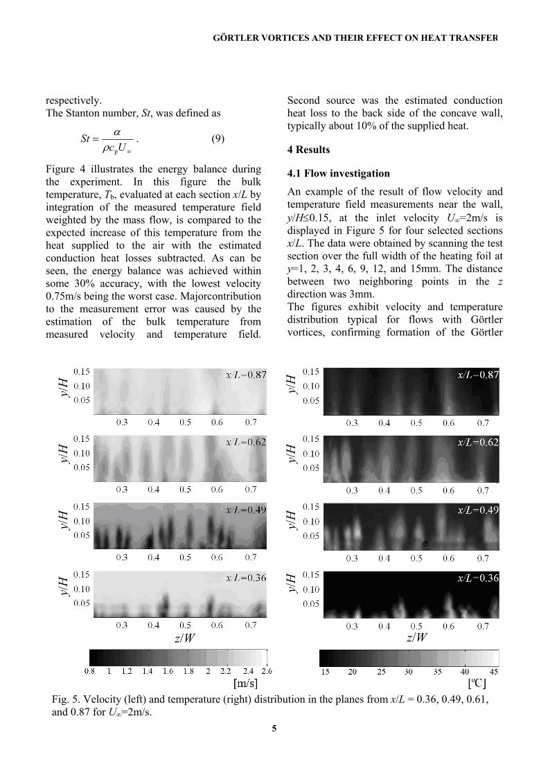
Figure 4 illustrates the energy balance during the experiment. In this figure the bulk temperature, Tb, evaluated at each section x/L by integration of the measured temperature field weighted by the mass flow, is compared to the expected increase of this temperature from the heat supplied to the air with the estimated conduction heat losses subtracted. As can be seen, the energy balance was achieved within some 30% accuracy, with the lowest velocity 0.75m/s being the worst case. Majorcontribution to the measurement error was caused by the estimation of the bulk temperature from measured velocity and temperature field.

Second source was the estimated conduction heat loss to the back side of the concave wall, typically about 10% of the supplied heat.

4 Results

4.1 Flow investigation

An example of the result of flow velocity and temperature field measurements near the wall, y/H≤0.15, at the inlet velocity U∞=2m/s is displayed in Figure 5 for four selected sections x/L. The data were obtained by scanning the test section over the full width of the heating foil at y=1, 2, 3, 4, 6, 9, 12, and 15mm. The distance between two neighboring points in the z direction was 3mm. The figures exhibit velocity and temperature distribution typical for flows with Görtler vortices, confirming formation of the Görtler

Fig. 5. Velocity (left) and temperature (right) distribution in the planes from x/L = 0.36, 0.49, 0.61, and 0.87 for U∞=2m/s.

y/H

y/H

y/H

y/H

z/W

y/H

y/H

y/H

y/H

z/W

6

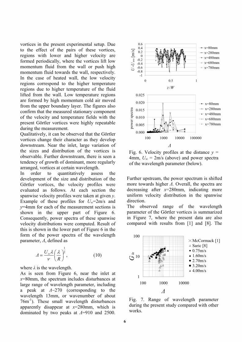
vortices in the present experimental setup. Due to the effect of the pairs of these vortices, regions with lower and higher velocity are formed periodically, where the vortices lift low momentum fluid from the wall or push high momentum fluid towards the wall, respectively. In the case of heated wall, the low velocity regions correspond to the higher temperature regions due to higher temperature of the fluid lifted from the wall. Low temperature regions are formed by high momentum cold air moved from the upper boundary layer. The figures also confirm that the measured stationary component of the velocity and temperature fields with the present Görtler vortices were highly repeatable during the measurement. Qualitatively, it can be observed that the Görtler vortices change their character as they develop downstream. Near the inlet, large variation of the sizes and distribution of the vortices is observable. Further downstream, there is seen a tendency of growth of dominant, more regularly arranged, vortices at certain wavelength. In order to quantitatively assess the development of the size and distribution of the Görtler vortices, the velocity profiles were evaluated as follows. At each section the spanwise velocity profiles were taken at given y. Example of these profiles for U∞=2m/s and y=4mm for each of the measurement sections is shown in the upper part of Figure 6. Consequently, power spectra of these spanwise velocity distributions were computed. Result of this is shown in the lower part of Figure 6 in the form of the power spectra of the wavelength parameter, Λ, defined as

21

= ∞

RU

Λ λνλ , (10)

where λ is the wavelength. As is seen from Figure 6, near the inlet at x=80mm, the spectrum includes disturbances at large range of wavelength parameter, including a peak at Λ~270 (corresponding to the wavelength 13mm, or wavenumber of about 76m-1). These small wavelength disturbances apparently disappear at x=280mm, which is dominated by two peaks at Λ=910 and 2500.

Further upstream, the power spectrum is shifted more towards higher Λ. Overall, the spectra are decreasing after x=280mm, indicating more uniform velocity distribution in the spanwise direction. The observed range of the wavelength parameter of the Görtler vortices is summarized in Figure 7, where the present data are also compared with results from [1] and [8]. The

1

10

100

100 1000 10000

Λ

Gδr

McCormack [1]Saric [8]0.75m/s1.60m/s2.70m/s3.20m/s4.00m/s

Fig. 7. Range of wavelength parameter during the present study compared with other works.

-1-0.8-0.6-0.4-0.2

00.20.40.6

0 0.5 1

z /W

U-U

ave [

m/s

] x=80mmx=280mmx=480mmx=680mmx=780mm

0.000

0.005

0.010

0.015

0.020

0.025

100 1000 10000 100000

pow

er s

pect

ra

x=80mmx=280mmx=480mmx=680mmx=780mm

Fig. 6. Velocity profiles at the distance y = 4mm, U∞ = 2m/s (above) and power spectra of the wavelength parameter (below).

Λ

7


vertical axis represents the Görtler number defined as

21

δr

= ∞

RUG rr δνδ , (11)

where δr is the boundary layer thickness parameter, defined in accordance with [8] as

21

⋅=

∞Ux

rνδ . (12)

4.2 Heat transfer results The effect of the Görtler vortices and their downstream development on heat transfer on the concave wall can be qualitatively estimated from the visualization of the uniformly heated wall temperature by thermochromic foil shown in Figure 8 for inlet velocities 1.6 and 2.7m/s. In agreement with the previously shown velocity and temperature field measurements, larger number of smaller disturbances is observed near the inlet to the test section, with gradual growth of dominant larger scale vortices further downstream. The substantial variation of the wall temperature in the spanwise direction also indicates significant variation of the local heat transfer coefficient. The heat transfer distribution was evaluated quantitatively by experiments consisting of detailed measurement of the velocity and temperature fields in the central part of the test section in the range of 0.45<z/W<0.55 with pitch 3mm, and across its full height at z=1, 2, 4, 8, 16, 30, 50, 70, 80mm. Simultaneously, wall temperature of the heater and heat conduction losses through the concave wall were measured by embedded thermocouples. Results of the Nusselt number distribution for five inlet velocities, U∞=0.75, 1.6, 2.7, 3.2, and 4m/s, is shown in Figure 9. The downstream development of the average heat transfer coefficient at each section is shown in Figure 10 for the same set of velocities. The present results are also compared with the values of the heat transfer coefficient for flat plate for laminar and turbulent flow, evaluated from the correlations given by Equations (7) and (8),

Fig. 9. Nu distribution on the concave wall. From top, the inlet velocities are 0.75, 1.6, 2.7, 3.2, and 4m/s.

Fig. 8. Wall temperature visualization for U∞=1.6m/s (left) and 2.7m/s (right).

x/L x/L

z/W

z/W

Nu:

x/L

Z/w

Z/

w

Z/w

Z/

w

Z/w

8

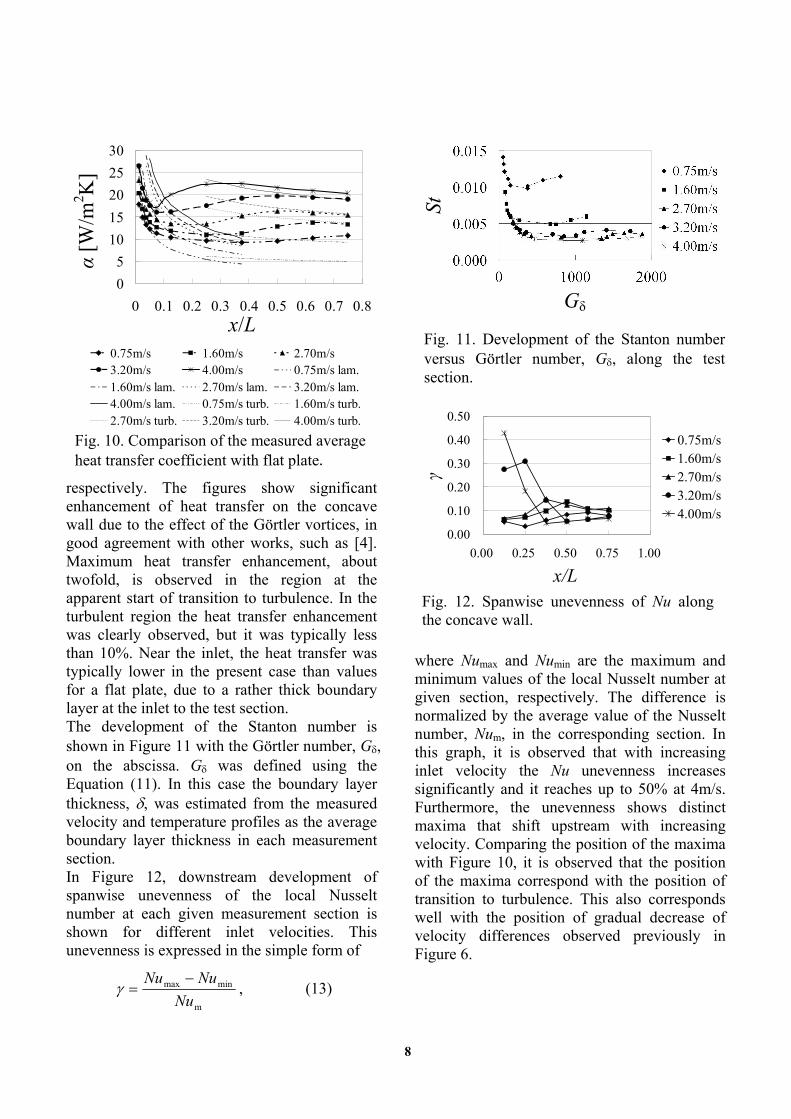
respectively. The figures show significant enhancement of heat transfer on the concave wall due to the effect of the Görtler vortices, in good agreement with other works, such as [4]. Maximum heat transfer enhancement, about twofold, is observed in the region at the apparent start of transition to turbulence. In the turbulent region the heat transfer enhancement was clearly observed, but it was typically less than 10%. Near the inlet, the heat transfer was typically lower in the present case than values for a flat plate, due to a rather thick boundary layer at the inlet to the test section. The development of the Stanton number is shown in Figure 11 with the Görtler number, Gδ, on the abscissa. Gδ was defined using the Equation (11). In this case the boundary layer thickness, δ, was estimated from the measured velocity and temperature profiles as the average boundary layer thickness in each measurement section. In Figure 12, downstream development of spanwise unevenness of the local Nusselt number at each given measurement section is shown for different inlet velocities. This unevenness is expressed in the simple form of

m

minmax

NuNuNu −

=γ , (13)

where Numax and Numin are the maximum and minimum values of the local Nusselt number at given section, respectively. The difference is normalized by the average value of the Nusselt number, Num, in the corresponding section. In this graph, it is observed that with increasing inlet velocity the Nu unevenness increases significantly and it reaches up to 50% at 4m/s. Furthermore, the unevenness shows distinct maxima that shift upstream with increasing velocity. Comparing the position of the maxima with Figure 10, it is observed that the position of the maxima correspond with the position of transition to turbulence. This also corresponds well with the position of gradual decrease of velocity differences observed previously in Figure 6.

Fig. 11. Development of the Stanton number versus Görtler number, Gδ, along the test section.

05

1015202530

0 0.1 0.2 0.3 0.4 0.5 0.6 0.7 0.8

0.75m/s 1.60m/s 2.70m/s3.20m/s 4.00m/s 0.75m/s lam.1.60m/s lam. 2.70m/s lam. 3.20m/s lam.4.00m/s lam. 0.75m/s turb. 1.60m/s turb.2.70m/s turb. 3.20m/s turb. 4.00m/s turb.

Fig. 10. Comparison of the measured average heat transfer coefficient with flat plate.

0.00

0.10

0.20

0.30

0.40

0.50

0.00 0.25 0.50 0.75 1.00

x/L

γ0.75m/s1.60m/s2.70m/s3.20m/s4.00m/s

Fig. 12. Spanwise unevenness of Nu along the concave wall.

St

Gδ x/L

α [W

/m2 K

]

9


5 Discussion

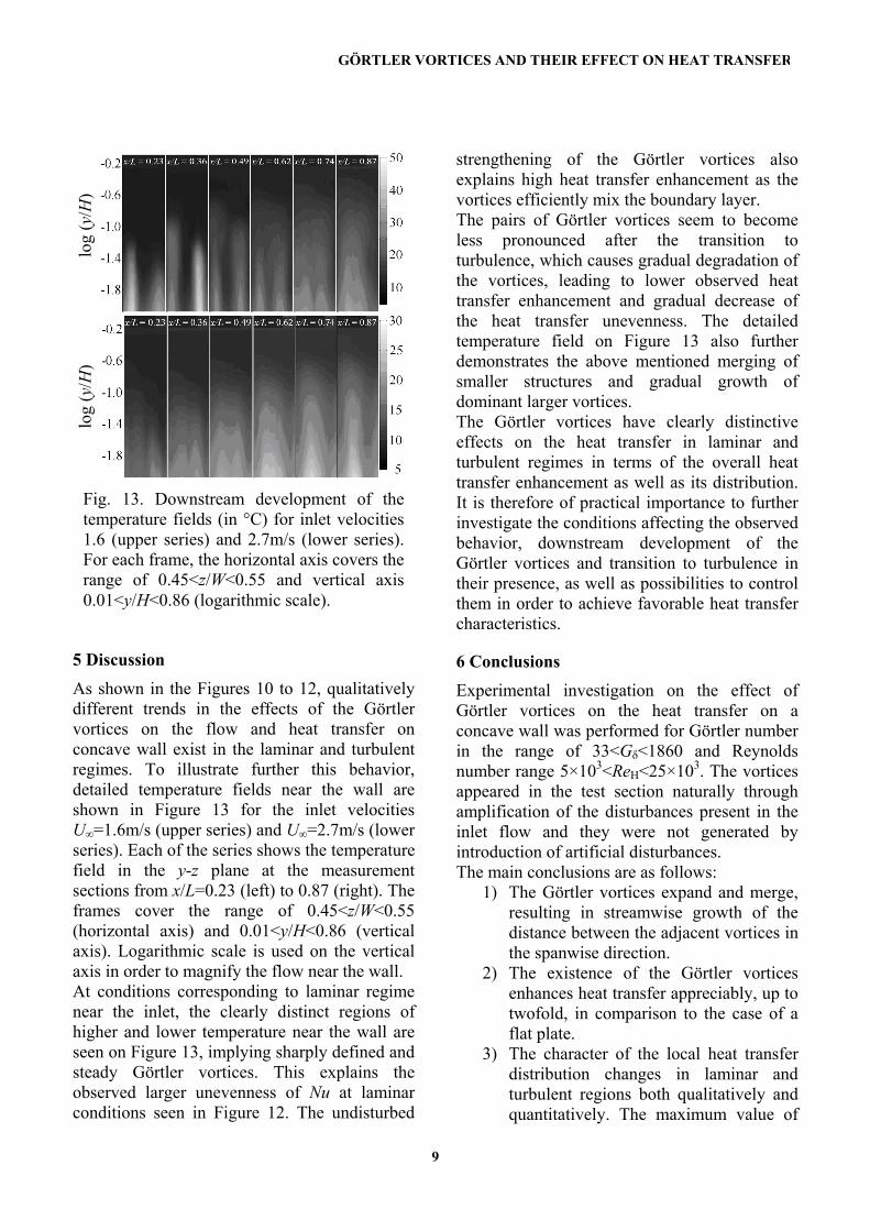
As shown in the Figures 10 to 12, qualitatively different trends in the effects of the Görtler vortices on the flow and heat transfer on concave wall exist in the laminar and turbulent regimes. To illustrate further this behavior, detailed temperature fields near the wall are shown in Figure 13 for the inlet velocities U∞=1.6m/s (upper series) and U∞=2.7m/s (lower series). Each of the series shows the temperature field in the y-z plane at the measurement sections from x/L=0.23 (left) to 0.87 (right). The frames cover the range of 0.45<z/W<0.55 (horizontal axis) and 0.01<y/H<0.86 (vertical axis). Logarithmic scale is used on the vertical axis in order to magnify the flow near the wall. At conditions corresponding to laminar regime near the inlet, the clearly distinct regions of higher and lower temperature near the wall are seen on Figure 13, implying sharply defined and steady Görtler vortices. This explains the observed larger unevenness of Nu at laminar conditions seen in Figure 12. The undisturbed

strengthening of the Görtler vortices also explains high heat transfer enhancement as the vortices efficiently mix the boundary layer. The pairs of Görtler vortices seem to become less pronounced after the transition to turbulence, which causes gradual degradation of the vortices, leading to lower observed heat transfer enhancement and gradual decrease of the heat transfer unevenness. The detailed temperature field on Figure 13 also further demonstrates the above mentioned merging of smaller structures and gradual growth of dominant larger vortices. The Görtler vortices have clearly distinctive effects on the heat transfer in laminar and turbulent regimes in terms of the overall heat transfer enhancement as well as its distribution. It is therefore of practical importance to further investigate the conditions affecting the observed behavior, downstream development of the Görtler vortices and transition to turbulence in their presence, as well as possibilities to control them in order to achieve favorable heat transfer characteristics.

6 Conclusions Experimental investigation on the effect of Görtler vortices on the heat transfer on a concave wall was performed for Görtler number in the range of 33<Gδ<1860 and Reynolds number range 5×103<ReH<25×103. The vortices appeared in the test section naturally through amplification of the disturbances present in the inlet flow and they were not generated by introduction of artificial disturbances. The main conclusions are as follows:

1) The Görtler vortices expand and merge, resulting in streamwise growth of the distance between the adjacent vortices in the spanwise direction.

2) The existence of the Görtler vortices enhances heat transfer appreciably, up to twofold, in comparison to the case of a flat plate.

3) The character of the local heat transfer distribution changes in laminar and turbulent regions both qualitatively and quantitatively. The maximum value of

Fig. 13. Downstream development of the temperature fields (in °C) for inlet velocities 1.6 (upper series) and 2.7m/s (lower series). For each frame, the horizontal axis covers the range of 0.45<z/W<0.55 and vertical axis 0.01<y/H<0.86 (logarithmic scale).

log

(y/H

)

log

(y/H

)

10

the Nusselt number spanwise unevenness, γ, increases and the position of the maximum gradually shifts upstream with increasing Reynolds number, from γ less than 10% at x/L=0.625 for ReH=5×103 to γ=43% at x/L=0.125 for ReH=25×103.

Nomenclature A area, [m2]; b concave wall thickness, [m]; cp specific heat at constant pressure,

[J/(kg·K)]; kair air thermal conductivity, [W/(m·K)]; ks Styroform thermal conductivity,

[W/(m·K)]; kw concave wall thermal conductivity,

[W/(m·K)]; q& heat flux, [W/m2];

condq& conductive heat loss, [W/m2];

fq& supplied heat flux, [W/m2]; x distance from the inlet, [m]; y radial distance from the concave wall,

[m]; z spanwise distance, [m]; Gδ Görtler number based on boundary

layer thickness, [-]; Gδr Görtler number based on boundary

layer thickness parameter, [-]; Gθ Görtler number based on boundary

layer momentum thickness, [-]; H duct height, [m]; IT turbulence intensity, [%]; L duct length, [m]; Nu Nusselt number, [-]; Nufp Nusselt number on a flat plate, [-]; Num spanwise averaged Nusselt number, [-]; R wall radius of curvature, [m]; ReH Reynolds number, [-]; Rex Reynolds number based on distance

from the inlet to the test section, [-]; St Stanton number, [-]; Tb bulk temperature, [°C]; Tback temperature on the back of the test

section, [°C]; Tw wall temperature, [°C]; Twa average wall temperature, [°C];

T∞ free stream (inlet) temperature, [°C]; U velocity, [m/s]; Uave average velocity, [m/s]; U∞ freestream (inlet) velocity, [m/s]; W duct width, [m]; α heat transfer coefficient, [W/(m2K)]; γ dimensionless unevenness of Nu (Eq.

13), [-]; δ boundary layer thickness, [m]; δr boundary layer thickness parameter,

[m]; θ boundary layer momentum thickness,

[m]; λ wavelength of vortices formation, [m]; ν kinematic viscosity, [m2/s]; ρ density, [kg/m3]; Λ wavelength parameter, [-];

References [1] McCormack P D, Welker H and Kelleher M.

Taylor-Görtler vortices and their effect on heat transfer. ASME J. Heat Transfer, Vol. 92, pp 101-112, 1970.

[2] Umur H and Karagöz I. An investigation of external flows with various pressures and surfaces. Int. Comm. Heat Mass Transfer, Vol. 26, No. 3, pp 411- 419, 1999.

[3] Umur H. Flow and heat transfer with pressure gradients, Reynolds number and surface curvature. Int. Comm. Heat Mass Transfer, Vol. 27, No. 3, pp 397-406, 2000.

[4] Toé R, Ajakh A and Peerhossaini H. Heat transfer enhancement by Görtler instability. Int. J. Heat Fluid Flow, Vol. 23, pp 194-204, 2002.

[5] Peerhossaini H and Wesfreid J E. On the inner structure of Görtler vortices. Int. J. Heat Fluid Flow, Vol. 9, pp 12-18, 1988.

[6] Ozalp A A and Umur H. An experimental investigation of the combined effect of surface curvature and streamwise pressure gradients both in laminar and turbulent flows. Int. J. Heat Mass Transfer, Vol. 39, DOI 10.1007/S00231-003-0413-4, pp 869-876, 2003.

[7] Guo Y and Finlay W H. Wavenumber selection and irregularity of spatially developing nonlinear Dean and Görtler vortices. J. Fluid Mech., Vol. 264, No. 1, pp 1- 40, 1994.

[8] Saric W. Görtler vortices. Annu. Rev. Fluid Mech. 26, pp 379-409, 1994.

GÖRTLER VORTICES AND THEIR EFFECT ON HEAT...

Documents

Transcript of GÖRTLER VORTICES AND THEIR EFFECT ON HEAT...