Growth model of agri-food production - AgEcon...

Growth model of agri-food production

Agnieszka Bezat-Jarzębowska

Włodzimierz Rembisz

Agata Sielska

nr 13.1Warsaw 2012

nW

13.1nr2012arsaw W

Growth model of agri-food production

Warsaw 2012

Growth modelof agri-foodproduction

Authors:

dr inż. Agnieszka Bezat-Jarzębowska

prof. dr hab. Włodzimierz Rembisz

mgr Agata Sielska

This publication was prepared as a contribution to the research on the following subject Economic modeling in the analysis of competitive growth of agri-food sector within the framework of the research task Equilibrium growth of domestic agri-food sector and its union and global competitiveness

The purpose of this research was to develop an economic model of agri-food sector` growth. The model presented includes the demand side based on behaviors of consumer on retail as well as a food processor on farm markets as opposite to the supply side based on farm producer` behavior.

Reviewerdr Miros�aw Drygas

Translated by Contact Langvage Services

Cover Project AKME Projekty Sp. z o.o.

ISBN 978-83-7658-218-4

Instytut Ekonomiki Rolnictwa i Gospodarki �ywno�ciowej – Pa�stwowy Instytut Badawczy 00-950 Warszawa, ul. �wi�tokrzyska 20, skr. poczt. nr 984 tel.: (22) 50 54 444 faks: (22) 50 54 636 e-mail: [email protected] http://www.ierigz.waw.pl

Contents

Introduction ........................................................................................................... 7�

1. Consumer, agricultural producer and agri-food processors in the model ............... 9�

1.1. Consumers ............................................................................................... 9�

1.2. Agri-food processor ............................................................................... 28�

1.3. Agricultural producer ............................................................................ 33�

2. Role of the processor in the growth model of agri-food production ............... 35�

3. Growth factors of agricultural production in the developed model ................ 45�

3.1.�Changes in agricultural land resources and their productivity .................. 45�

3.2.�Growth rate of agricultural production .................................................. 52�

References ........................................................................................................... 66�

7

Introduction

Demand for finished food products provides market conditions for agri-food processors. They, in turn, create demand conditions for agricultural producers. This assumption constitutes the standpoint of analysis conducted in this work. That is also the structure of the growth model of agri-food production, which is central herein. The growth model, at this stage, is subjected to a preliminary empirical ver-ification. Due to the fact that the presented formulas and mathematical objects in-cluded in the model are mainly analytical rather than estimating, empirical study is relevant mostly to illustrate and confirm the assumptions and analytical solutions adopted in the model.

Demand conditions, in the case of agricultural raw materials and agricultural producers that produce them, are: firstly, the final demand of consumers, and sec-ondly, the intermediate demand of agri-food processors. Both these entities, i.e. both the consumer and the processor shape the market situation of the grower.

Agri-food market in fact is comprised of two combined markets. First, the market of finished food products (goods) with own regularities of a general and specific nature. Second, the market of agricultural raw materials also with general and specific regularities typical of this market. Relationships and dependencies of a microeconomic nature between them will be presented in the first chapter,. which aims at outlining the background for further analysis. In the second part we raise the question of food processors and their impact on the producers through prices of agricultural raw materials. Chapter three is dedicated to the increase in agricultural production and the factors shaping it.

9

1. Consumer, agricultural producer and agri-food processors in the model

1.1. Consumers

Theoretical description of the agri-food market allows for identification of three entities whose interactions determine the market balance. In this perspective, we can distinguish consumers, agri-food processors and agricultural producers. They form a kind of circular flow of interdependent entities. The behaviour of each of them condi-tions the behaviour of others.

It is assumed that the conditions of consumer determine the equilibrium condi-tions of the producer (in this case, both agricultural producers and agri-food proces-sors). Therefore, one can assume that the balance of the consumer, i.e. the final pur-chaser of food, determines the balance of the agricultural producer and the agri-food processor, and that the balance of the processor determines the balance of the agricul-tural producer, assuming a correlation here, which results from the nature of manage-ment in the agri-food sector. With that in mind, the above interrelation can be translat-ed into foundations for our further analysis. Namely, the balance of the food and agri-cultural markets is a derivative of the consumer balance in the sense of maximizing its objective function (utility). Thus, it can be assumed that the level of income of agricul-tural producers is ultimately determined by the consumer who chooses between ac-quired value (quantity and price) of food in relation to the value of non-food goods1.

For the purposes of our analysis we divide consumed goods in two types: food and non-food goods2, as uniform goods.

Thus, in this context, with food and non-food goods, the conditional function of the consumer objective (mechanism of behaviour) can be written as follows:

max),( ��PU (1.1) where:

�P C�CPm �� (1.2) where: U – consumer utility function, m – consumer income, budget limit, P – non-food consumer goods, PC – non-food consumer goods prices, � – agricultural food goods,

�C – prices of food of agricultural origin.

1Of course, the issue here is the optimal choice to maximize one’s own utility function at a given time, but also indirect interim choice, which is not analysed herein. In microeconomic terms, the issue is presented in the form of conditional optimisation of the consumer choice. 2 We adopt microeconomic classification, according to which a good is what the consumer buys, and what is produced by the manufacturer is defined as the product with the same value of use. This is expressed by the necessary condition of manufacturer rational behaviour in the sense that he produces what is purchased by the consumer, i.e. the product becomes a good when it is purchased. In other words: the producer produces what is in demand, taking into account other considerations, such as prices, preferences, etc. Cf. W. Rembisz, A. Sielska, Mikroekonomia – zarys w uj�ciu analitycznym, Vizja Press&IT, Warsaw 2011.

10

The solution to optimization tasks defined in this way, allows for explaining the mechanism of consumer behaviour. This determines the demand notified by the con-sumers for food products from agricultural sources and allows to determine the ap-proximate size of the demand. Therefore, with the condition given by the formula (1.2) it is easy to determine the demand for food3:

PCC

Cm�

�

P

�

�� (1.3)

As can be seen in the above, the demand for food is determined by the two di-rect economic factors associated with the market category. Firstly, the demand is de-termined by the level of real prices of food measured by their relationship to consumer spending, that is:

�Cm (1.4)

The second factor included in the above formula is the relationship of food to the prices of non-food products - industrial products (and others) and their level of consumption at any given time, that is:

PCC

�

P

(1.5)

As one can see, there are no high or low prices, there are only relatively high or relatively low prices in relation to income or in relation to the prices of other goods. Both of these indicators reflect the real level of food prices. It may be noted that the lev-el of real prices defined in this way is a reflection of efficiency relationships occurring between producers in the economy and its various sectors. The important conclusion following from the above, is that the real level of food prices is not only dependent on agricultural producers or, to put it more broadly, on food producers. It depends on the

3 If this formula (1.3) is differentiated, we would obtain rates of changes of the values con-tained on the right side, i.e.:

tmm 1�

�

the growth rate of income,

tCC

�

� 1�

�rate of increase in food prices,

tCC

P

P 1�

�

which are

easily converted into indexes.

This is easy to illustrate in the conventional analysis. Relevant

data were compared in the table below, they illustrate the economic sense of the formula (1.3) and (1.4) and (1.5), showing the food getting relatively cheaper in relation to income, and the lack of significant change in real prices, i.e. the ratio of food prices to prices of other products, which is shown analytically by the first quotient on the right side (1.3). These issues will be revisited in the analytical approach developed in the second part of the research.

Indicators (indexes) of the increase in prices of non-food and food products and salary (income) increases in 2000-2010

Item

2000-2003

2004-2006

2007-2009

2010 2004-2010

2000-2010

Consumer goods and services 119.3 106.8 110.5 102.6 121.1 144.5 Food and non-alcoholic bever-ages 113.5 109.2 115.8 102.7 129.9

147.4

Wages and salaries in the enter-prise sector 128.6 113.8 125.5 103.3 147.6

189.8

Source: CSO data.

11

income of real consumers, which is known to be determined by the productivity of la-bour in the economy, especially in the non-agricultural sectors”4.

Ratio of non-food product prices to food product prices is expressed as a coeffi-

cient: �

P

CC that reflects5 the possibility of substitution that occurs between these two

types of goods. By differentiating the utility function given by (1.1) under the condi-tion (1.2) we obtain:

P

�

CC

�U

PU

P�

��

��

��

�� (1.6)

This means that the consumer balance6 is determined by the reciprocal of the ra-tio of marginal utility to the inverse relationship of prices for those goods, namely:

�UC� ��

�

(1.7)

PUCP ��

�

(1.8)

Note that if the condition defined by equality (1.6) is not satisfied, the consumer will change the selected items, substituting certain goods with others, to bring new relative relationships between utility and prices, according to the scheme, which can be written as:

��

��UC�

(1.9)

��

�PUCP

(1.10)

In the described case of discrepancy between goods’ prices and marginal utili-ties some role is played also by agricultural producers and agri-food processors in-volved in the production of food products. If the price of food products on the retail

market is higher than their utility to the consumer (�UC� ��

), the consumer will be

inclined to reduce the amount of purchased products, the producers and processors can, however, in this case, take action to increase the utility of goods. This process of substitution (replacement of demand for goods characterised by a relatively higher price and lower utility with demand for goods with higher utility and lower price) will continue until the equality (1.6) is satisfied7. Thus we have, the following:

P� CMP

CM� �� , (1.11)

4 W. Rembisz, Mikroekonomiczne podstawy wzrostu dochodów producentów rolnych, Vizja Press&IT, Warsaw 2007, p. 14. 5As can be seen by solving the task of maximizing consumer utility function with constant budget limit (i.e. with unchanged income). 6The optimal basket of food and non-food goods selected by the consumer. 7Of course, there are certain limits, it is not possible to consume only non-food goods, while the opposite case is possible.

12

Both price relationships shown in the above formulas (1.4) and (1.5) are exem-plifications of regularities associated with the Engel law. In the context of this law, the most important relationship is the relationship between the demand for food and the income. This is illustrated by the demand function:

)(mf� D � (1.12) where: D� – demand for food products.

The share of expenditure on food in consumer spending is important in shaping the demand for food, in the context of the law. With (1.2) this ratio is in the following form:

mC�

m ��

�� )(mf� D � (1.13)

This index is illustrated empirically (tables 1.6, 1.7 and graph in Figure 1.12). It should decrease along with the increase in income. It is also an expression (illustra-tion) of increasing prosperity, when accompanied by an increase in the value of food consumption per capita, which is also illustrated empirically (Table 1.7).

Knowledge of flexibility is important for the study of the formation of the level of demand for products of agricultural producers and services of agri-food processors. This can be written as8:

1)1( �� DZ�

DP� EmEm (1.14)

DPE – income elasticity of demand for non-food products, D�E – income elasticity of demand for food products.

Elasticity is also important to estimate the total revenue of the producer (defined as the product of prices and quantities of products) and the possibility of increasing it9.

It is assumed10 now that the possibilities of increase in prices of agri-food prod-ucts are small. This is due to the low income elasticity of demand for food products (presented in Table 1.1 also in relation to non-food goods) in the analysed countries of the European Union. These elasticises were at a similar level, but the elasticity of de-mand for food products was the highest in the Polish market. This illustrates regulari-ties mentioned above. Demand for food was less elastic in relation to changes in in-come than in case of other goods. Therefore this variable (i.e. income through elastici-ty) should be included in the demand conditions of growth in agri-food production. The values of this ratio for Poland are also shown in Figure 1.1. 8 Rembisz W., Mikroekonomiczne…, op.cit. p. 19. 9According to W. Tomek, K. Robinson, it can be noted that "If demand is elastic in consid-eration of price, the price and total revenue vary inversely. The increase in price causes a decrease in total revenue, while its decline - a drop in revenues. This is a direct consequence of the definition of elastic demand (...)". On the other hand, if demand is inelastic, and the property is usually attributable to the demand for food products, "one must expect that with other factors unchanged, the price and total revenue of the producer will change in a manner directly proportional". The same authors also cite words of H.A. Wallace, who in 1915 con-cluded that "from the principles of demand it follows that agriculture is punished for too high level of production and rewarded for too low level of production" Tomek W.G., Robinson K.L, Kreowanie cen artyku�ów rolnych, PWN, Warsaw, 2001, p. 38. 10 W. Rembisz, Mikroekonomiczne podstawy wzrostu dochodów producentów rolnych, Vizja Press&IT, Warsaw 2007.

13

Table 1.1. Comparison of income elasticity of demand for selected categories of goods and services in the analysed countries of the European Union in 2005

Goods

Country Food

, bev

erag

es

and

toba

cco

Clo

thin

g an

d fo

otw

ear

Hom

e fu

rnis

hing

s an

d ho

useh

old

mai

nten

ance

Furn

iture

Hea

lth

Tran

spor

t and

co

mm

unic

atio

n

Leis

ure

Educ

atio

n

Oth

er

Poland 0.628 0.965 1.065 1.049 1.282 1.147 1.359 0.919 1.285 Hungary 0.612 0.965 1.064 1.049 1.273 1.145 1.345 0.918 1.276 Czech Republic 0.583 0.965 1.063 1.048 1.261 1.141 1.325 0.917 1.263

Sweden 0.513 0.964 1.062 1.047 1.239 1.134 1.293 0.914 1.241 Italy 0.508 0.964 1.062 1.047 1.238 1.134 1.291 0.914 1.240 Belgium 0.507 0.964 1.062 1.047 1.238 1.134 1.291 0.914 1.240 Spain 0.503 0.964 1.062 1.047 1.237 1.134 1.289 0.914 1.239 France 0.492 0.964 1.062 1.047 1.235 1.133 1.286 0.914 1.236 Germany 0.477 0.964 1.061 1.047 1.232 1.132 1.281 0.913 1.233

Source: USDA.

Figure 1.1. Income elasticity of demand for different categories of goods in Poland in 2005

Source: Author’s own compilation based on the data from the USDA.

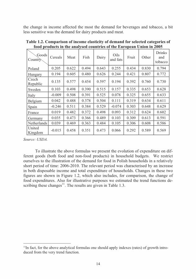
Significant differences in the evolution of income elasticity of demand refer to

the cereal products and fats. The relevant data are presented in Table 1.2. There is a similarity in this field in Poland and in the Czech Republic and Hungary. In each case,

14

the change in income affected the most the demand for beverages and tobacco, a bit less sensitive was the demand for dairy products and meat.

Table 1.2. Comparison of income elasticity of demand for selected categories of

food products in the analysed countries of the European Union in 2005

Goods Country Cereals Meat Fish Dairy Oils

and fats Fruit Other Drinks

and tobacco

Poland 0.205 0.622 0.494 0.643 0.255 0.434 0.830 0.794 Hungary 0.194 0.605 0.480 0.626 0.244 0.421 0.807 0.772 Czech Republic 0.135 0.577 0.454 0.597 0.194 0.392 0.760 0.730

Sweden 0.103 0.498 0.390 0.515 0.157 0.335 0.653 0.628 Italy -0.009 0.508 0.391 0.525 0.078 0.325 0.655 0.633 Belgium 0.042 0.488 0.378 0.504 0.111 0.319 0.634 0.611 Spain -0.246 0.511 0.384 0.529 -0.074 0.303 0.648 0.629 France 0.019 0.482 0.372 0.498 0.093 0.312 0.624 0.602 Germany 0.035 0.473 0.366 0.489 0.103 0.309 0.613 0.591 Netherlands 0.039 0.469 0.363 0.484 0.105 0.306 0.608 0.586 United Kingdom -0.015 0.458 0.351 0.473 0.066 0.292 0.589 0.569

Source: USDA.

To illustrate the above formulas we present the evolution of expenditure on dif-

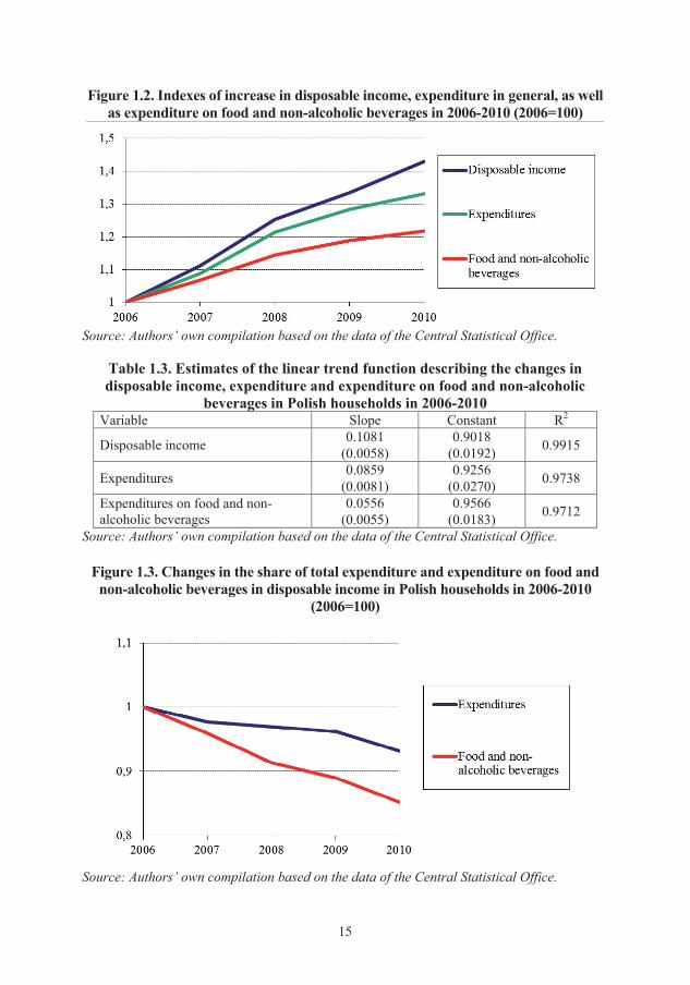
ferent goods (both food and non-food products) in household budgets. We restrict ourselves to the illustration of the demand for food in Polish households in a relatively short period of time: 2006-2010. The relevant period was characterised by an increase in both disposable income and total expenditure of households. Changes in these two figures are shown in Figure 1.2, which also includes, for comparison, the change of food expenditures. Also for illustrative purposes we estimated the trend functions de-scribing these changes11. The results are given in Table 1.3.

11In fact, for the above analytical formulas one should apply indexes (rates) of growth intro-duced from the very trend function.

15

Figure 1.2. Indexes of increase in disposable income, expenditure in general, as well as expenditure on food and non-alcoholic beverages in 2006-2010 (2006=100)

Source: Authors’ own compilation based on the data of the Central Statistical Office.

Table 1.3. Estimates of the linear trend function describing the changes in disposable income, expenditure and expenditure on food and non-alcoholic

beverages in Polish households in 2006-2010 Variable Slope Constant R2

Disposable income 0.1081 0.9018 0.9915 (0.0058) (0.0192)

Expenditures 0.0859 0.9256 0.9738 (0.0081) (0.0270) Expenditures on food and non-alcoholic beverages

0.0556 0.9566 0.9712 (0.0055) (0.0183) Source: Authors’ own compilation based on the data of the Central Statistical Office.

Figure 1.3. Changes in the share of total expenditure and expenditure on food and

non-alcoholic beverages in disposable income in Polish households in 2006-2010 (2006=100)


16

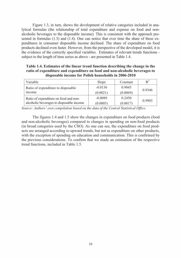
Figure 1.3, in turn, shows the development of relative categories included in ana-lytical formulas (the relationship of total expenditure and expense on food and non-alcoholic beverages to the disposable income). This is consistent with the approach pre-sented in formulas (1.3) and (1.4). One can notice that over time the share of these ex-penditures in consumer disposable income declined. The share of expenditure on food products declined even faster. However, from the perspective of the developed model, it is the evidence of the correctly specified variables. Estimates of relevant trends functions - subject to the length of time series as above - are presented in Table 1.4.

Table 1.4. Estimates of the linear trend function describing the change in the ratio of expenditure and expenditure on food and non-alcoholic beverages to

disposable income for Polish households in 2006-2010

Variable Slope Constant R2 Ratio of expenditure to disposable income

-0.0136 0.9045 0.9346

(0.0021) (0.0069) Ratio of expenditure on food and non-alcoholic beverages to disposable income

-0.0089 0.2450 0.9903

(0.0005) (0.0017) Source: Authors’ own compilation based on the data of the Central Statistical Office.

The figures 1.4 and 1.5 show the changes in expenditure on food products (food

and non-alcoholic beverages) compared to changes in spending on non-food products (in broad categories used by the CSO). As one can see, the expenditure on food prod-ucts are arranged according to upward trends, but not as expenditure on other products, with the exception of spending on education and communication. This is confirmed by the previous considerations. To confirm that we made an estimation of the respective trend functions, included in Table 1.5.

Figu

re 1

.4. C

hang

es in

exp

endi

ture

of P

olis

h ho

useh

olds

on

food

and

sele

cted

non

-foo

d pr

oduc

ts in

200

6-20

10 (a

)

Sour

ce: A

utho

rs’ o

wn

com

pila

tion

base

d on

the

data

of t

he C

entr

al S

tatis

tical

Offi

ce.

��

Fi

gure

1.5

. Cha

nges

in e

xpen

ditu

re o

f Pol

ish

hous

ehol

ds o

n fo

od a

nd se

lect

ed n

on-f

ood

prod

ucts

in 2

006-

2010

(b)

Sour

ce: A

utho

rs’ o

wn

com

pila

tion

base

d on

the

data

of t

he C

entr

al S

tatis

tical

Offi

ce.

��

19

Table 1.5. Estimates of the linear trend function describing the changes in expenditure on food goods and non-food services in Polish households

in 2006-2010 Type of goods Slope Intercept R2

Food and non-alcoholic beverages

0.0556 0.9566 0.9712

(0.0055) (0.0183)

Home furnishings and household maintenance

0.0874 0.9752 0.8456

(0.0216) (0.0715)

Education 0.0472 0.9511

0.8580 (0.0111) (0.0368)

Health 0.0809 0.9364

0.9292 (0.0129) (0.0428)

Restaurants and hotels 0.1499 0.8046

0.9762 (0.0135) (0.0448)

Housing and energy 0.0985 0.8679

0.9610 (0.0115) (0.0380)

Clothing and footwear 0.0697 0.9782

0.8763 (0.0151) (0.0501)

Communication 0.0338 0.9879

0.8398 (0.0085) (0.0282)

Leisure and, culture 0.1278 0.9050

0.9574 (0.0156) (0.0516)

Source: Authors’ own compilation based on the data of the Central Statistical Office. Table 1.6 presents estimates of the trend function for expenditure on food prod-

ucts. As one can see, they were, in line with expectations, rising trends. It is clearly an expression of the growing prosperity - both increase in food consumption, as well as favourable changes in its structure, if one observes and illustrates increase in well-being in such a simple way. Adjustments of accepted trend functions to the real data are very good.

Despite the above-mentioned changes, the share of expenditure on individual food items in expenditure on food products remained - as shown by figures 1.6 and 1.7 - at a relatively constant level. One can therefore conclude that the demand for various food products remains stable. If this is due to the relatively high level of wealth, which does not lead to a further increase in food consumption (saturation level), the prospects for growth in agricultural production, as a response to a possible increase in demand, are small.

20

Table 1.6. Estimates of the linear trend function describing the changes in expenditure on different categories of food products in Polish households in 2006-2010

Type of goods Slope Intercept R2

Food 0.0535 0.9587

0.9686 (0.0056) (0.0185)

Bread and cereal-based foods 0.0658 0.9684

0.8725 (0.0145) (0.0482)

Oils and other fats 0.0390 0.9693

0.9009 (0.0075) (0.0248)

Fruit 0.0523 1.0029

0.7229 (0.0187) (0.0620)

Non-alcoholic beverages 0.0798 0.9316

0.9860 (0.0055) (0.0182)

Alcoholic beverages, tobacco and narcotics

0.0906 0.9151 0.9860

(0.0062) (0.0207) Source: Authors’ own compilation based on the data of the Central Statistical Office.

As a side note, it can be seen that values included in Figure 1.6 and 1.7 show

the evolution of relatively healthy consumption patterns. This is not good news for domestic producers, in view of the analysis of the developed model and the Heady’s convention. This means, in fact, that they cannot count on an increase in demand for traditional Polish products as a source of revenue growth both in size and price. These are the demand conditions resulting from the economic interpretation of these patterns. The above affects the value of the main indicator in the developed model, which is the rate of agricultural production ( r ), discussed in chapter three.

Figure 1.6. Share of expenditure on individual food products in the expenditure

on food in Polish households in 2006-2010


21

Figure 1.7. Changes in the share of expenditure on individual food products in spending on food in Polish households in 2006-2010


So much space was devoted to the final demand for food products, not only be-cause of the developed growth model for agri-food production. Research on the demand for food products are important in the theory of agricultural economics and agricultural policy. They allow for explaining important conditions of the income of agricultural pro-ducers. This is of practical importance to agricultural producers and agricultural policy. Indeed, the demand - its lower rate, is one of the factors that may limit the growth in the agri-food sector, including increase in the income of agricultural producers.

The increased spending on food products, observed in the EU countries, results from the greater role of processing - as will be discussed further on - and greater de-mand for highly processed products. It is important that now, thanks to technological advances, the possibilities of increase in production in relation to demand are virtually limitless. In this situation, the producers, seeking to improve the current level of prof-itability (and consequently revenue), have to change manufacturing techniques and improve the resulting efficiency12.

With microeconomic foundations, we can present the demand for finished food products in macro-economic terms. In this perspective, the demand for food products

12Improving efficiency is currently the only fundamental and least expensive to society way to improve the income of agricultural producers, including in relation to wages in other sectors of the economy. This is especially true of highly developed countries, including of course the EU countries analysed in this paper. The issue of production efficiency and its multidimen-sional nature is discussed in the last paragraph of the third chapter.

22

is determined by two values: population and the demand per capita13. Consequently, the demand for finished food goods in macroeconomic terms is determined in accord-ance with the following formula:

K

D

KD

L�L� �� (1.15)

K

DD

L�� L � (1.16)

DK

DL�L� �� (1.17)

where: D� – demand (consumption) for food products at the macroeconomic level (in the country); KL – population in the country; D

L� – average food consumption, de-mand per capita.

After appropriate transformations of the above equation we get an equation de-scribing the dynamic formula of demand:

D

D

K

KD

D

L

L

��

LL

��

��

�� (1.18)

where: D

D

�� –growth in demand for food in the country (total demand for food, the

demand for food as the aggregate total) ; K

K

LL� – rate of population or consumers

growth; D

D

L

L

��

– growth rate of demand per capita.

This approach is of course a consequence of the microeconomic approach, as dis-cussed and illustrated above, which related to the second component of the right-hand side

of (1.18), i.e. D

D

L

L

��

. In extended terms, in the above equations (1.15-1.18) we also take

into account factors that influence the development of the demand for food, including im-port and export of products, changes in the relation of prices of non-food products to the food products or the price elasticity of demand, as mentioned earlier. Macroeconomic formula in the extended form, with microeconomic variable components describing the mechanism of growth in demand, is suggested by other authors14. It in-cludes the rate of change in the ratio of prices for non-food products to food products, changes in the general level of consumption and the rate of per capita income and the cor-responding elasticity of demand:

13This is the approach which takes into account the consumer behaviour discussed above, re-sulting in the unit demand for food products, and the balance sheet recognition through add-ing the sum of consumers. 14Y. Yamaguchi, A. Binswanger, The role of Sectoral Technical Change in Development. University of Minnesota, pp. 85-7, 1985.

23

�C

�

P

�

P

K

KD

D

Emt

mE

CCt

CC

LtL

ata

�t�

��

��

��

�

��

��

��

��

�� 11111 (1.19)

where: at

a 1�

�� –shift of the demand function;

K

K

LtL 1

�� – rate of population growth;

��

��

�

��

��

�

P

�

P

CCt

CC

1 – changes in the ratio of prices of non-food products to prices of

food products; CE – price elasticity of demand;mt

m 1�

�� – rate of change in per capita

income; �E – income elasticity of demand. The equations of demand for food, in the above-presented form, are subject to

empirical parameterization and verification. Such attempts have been made in previous studies conducted by the IAFE15. Theoretical basis of food demand equations were shown earlier16.

It can be assumed that an increase in agricultural production is more and more dependent on the demand for processing services included in the finished food prod-ucts17. E.O. Heady noted that "in the course of further income growth, the consumer does not consume more physical quantities of food, does not buy more kilograms, but consumes food in other forms, better packaged, easy to prepare and eat" and "increase in spending on food per capita in U.S. is expressed... by the purchase of services relat-ed to the processing of food, and it is not associated with the size of agricultural prod-ucts. The increasing expenditure per capita in the United States are in particular re-lated to refrigeration, packaging and preparation of ready-to-eat food"18. J. Mellor and R. Ahmed, wrote that "in developed countries, the increase in food expenditures primarily represents the increase in expenditure on services related to the processing of agricultural products in the non-agricultural sector"19. The above fact is of appar-ent significance for the development of the demand-conditioned growth model of agri-food production. It is also confirmed by empirical research.

15 E.g. Rynek rolny - analizy tendencje oceny. Rynek �ywno�ciowy, K. �wietlik. 16 S. Figiel, W. Rembisz, Przes�anki wzrostu produkcji w sektorze rolno-spo�ywczym – uj�cie analityczne i empiryczne, IAFE-NRI, Warsaw 2009. 17 B. Senauer draws attention to this fact by writing "... food economy and food production is increasingly driven by factors on the side of consumption rather than on the side of agricul-tural production. More and more emphasis is moving from production to processing, distribu-tion and trade." This will be addressed later in the study. It is important that the consumer independence is increasing, the consumer is not condemned, as was the case in the previous system, to market deficiencies. This is the basis of rational consumer behaviour, which has an impact on moderate growth of demand for food. B. Senauer, Major Consumer Trends Affect-ing the US Food System, University of Minnesota, pp. 89-16, p.5. 18 E.O. Heady, Agricultural…, op. cit., p. 40. 19 J. Mellor, R. Ahmed, Agricultural Price Policy for Developing Countries, The Johns Hop-kings University Press, 1988, p. 61.

24

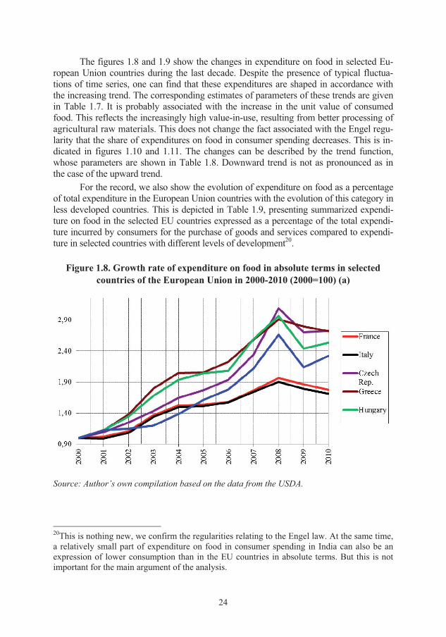
The figures 1.8 and 1.9 show the changes in expenditure on food in selected Eu-ropean Union countries during the last decade. Despite the presence of typical fluctua-tions of time series, one can find that these expenditures are shaped in accordance with the increasing trend. The corresponding estimates of parameters of these trends are given in Table 1.7. It is probably associated with the increase in the unit value of consumed food. This reflects the increasingly high value-in-use, resulting from better processing of agricultural raw materials. This does not change the fact associated with the Engel regu-larity that the share of expenditures on food in consumer spending decreases. This is in-dicated in figures 1.10 and 1.11. The changes can be described by the trend function, whose parameters are shown in Table 1.8. Downward trend is not as pronounced as in the case of the upward trend.

For the record, we also show the evolution of expenditure on food as a percentage of total expenditure in the European Union countries with the evolution of this category in less developed countries. This is depicted in Table 1.9, presenting summarized expendi-ture on food in the selected EU countries expressed as a percentage of the total expendi-ture incurred by consumers for the purchase of goods and services compared to expendi-ture in selected countries with different levels of development20.

Figure 1.8. Growth rate of expenditure on food in absolute terms in selected

countries of the European Union in 2000-2010 (2000=100) (a)

Source: Author’s own compilation based on the data from the USDA. 20This is nothing new, we confirm the regularities relating to the Engel law. At the same time, a relatively small part of expenditure on food in consumer spending in India can also be an expression of lower consumption than in the EU countries in absolute terms. But this is not important for the main argument of the analysis.

25

Figure 1.9. Growth rate of expenditure on food in absolute terms in selected countries of the European Union in 2000-2010 (2000=100) (b)


Figure 1.10. Rate of changes in the share of food expenditure in total expenditure in selected countries of the European Union in 2000-2010 (2000=100) (a)


26

Figure 1.11. Rate of changes in the share of food expenditure in total expenditure in selected countries of the European Union in 2000-2010 (2000=100) (b)


Table 1.7. Estimates of linear trend function describing the growth of expenditure on food in absolute terms in 2000-2010 for selected countries of

the European Union Country Slope Constant R2

United Kingdom 0.060 0.936 0.757 Germany 0.083 0.908 0.892 Netherlands 0.103 0.892 0.915 Sweden 0.098 0.856 0.916 Belgium 0.099 0.923 0.898 Spain 0.107 0.957 0.818 France 0.097 0.918 0.897 Italy 0.092 0.916 0.882 Czech Republic 0.206 0.671 0.915 Greece 0.197 0.877 0.938 Hungary 0.179 0.900 0.874 Poland 0.158 0.730 0.873

Source: Authors' own calculation according to the USDA data.

27

Table 1.8. Estimates of the linear trend function describing the percentage share of food expenditures in total expenditure in 2000-2010 for selected

countries of the European Union Country Slope Constant R2

United Kingdom 0.001 0.945 0.005 Germany -0.004 1.002 0.456

Netherlands 0.003 0.983 0.117 Sweden 0.001 1.011 0.036 Belgium -0.006 1.049 0.372

Spain -0.011 1.042 0.835 France -0.009 1.032 0.766 Italy -0.003 1.001 0.501

Czech Republic -0.016 1.002 0.722 Greece 0.001 1.096 0.006

Hungary -0.006 0.975 0.312 Poland -0.012 0.998 0.860

Source: Authors' own calculation according to the USDA data.

Table 1.9. Share of food expenditures in total expenditure in 2000-2010 for selected countries (in %)

Country

Year

Indi

a

Rus

sia

Rom

ania

Mac

edon

ia

Ukr

aine

Pola

nd

Ger

man

y

Fran

ce

Uni

ted

Kin

gdom

2000 41.75 46.76 34.89 29.40 46.49 22.83 11.49 14.12 9.62 2001 41.67 45.80 35.49 32.21 47.50 22.94 11.55 14.36 9.37 2002 39.48 41.70 34.78 33.52 45.99 21.77 11.53 14.43 9.15 2003 38.82 37.70 35.25 35.77 44.89 21.09 11.30 14.42 8.99 2004 34.36 36.00 33.47 33.12 43.88 21.22 11.18 14.08 8.83 2005 34.03 33.20 29.77 34.00 42.89 21.05 11.01 13.73 8.69 2006 32.52 31.60 29.11 32.87 42.28 20.88 10.99 13.44 8.62 2007 32.16 28.40 27.94 32.83 42.28 20.59 11.21 13.22 8.73 2008 30.52 29.10 28.04 32.99 42.23 20.43 11.36 13.47 9.14 2009 29.49 29.69 29.29 33.04 42.12 20.33 11.18 13.53 9.69 2010 27.69 29.00 29.69 32.92 46.86 20.20 11.05 13.18 9.70

Source: USDA.

28

1.2. Agri-food processor

As noted above, consumers report an increasing demand for services related to the processing of food, and more convenient form of consumption. Thus, the relation-ship between the agricultural producer and the consumer needs an additional link, i.e. the agri-food processor21. It creates a market demand for agricultural products as raw materials and supply on the market for finished food products. We have shown that in relation to the formula (1.14). Agricultural products, before they reach the final recipi-ent, are subject to increased processing, resulting in additional charges for these ser-vices. Agri-food processor responds to the preferences and needs of saving time on food consumption "by changing and adding to the form in which the product is ready for consumption and expanding the variety of products offered to the consumer from agricultural raw materials. Generally, it is associated with changes in the consumer utility function"22.

Changes in the share of individual links in the prices of products offered to the consumer results from the increased investment commitment of production factors in indirect links of the food chain between the producer and the consumer. P. Timmer pointed out the relationship between economic growth and changes in the share of each link of the marketing chain in the retail price of the product. At higher levels of development, when "the share of agriculture in employment is less than 20% and ex-penditure on food in total expenditure is lower than 30% (...) the share of agriculture in the value of the basket of food goods is very low due to the importance of processing and commercial services"23. Therefore, it is important to ask about the share of pro-cessing, trade and services in the value of finished food products purchased by con-sumers24.

The data contained in Table 1.10 allow us to conclude that all countries consid-ered in the present work are characterised by appropriate low levels of employment in the agricultural sector in relation to total employment, and lower expenditure on food in relation to spending on other consumer goods. The approximate empirical illustra-tion of the issues raised above can be found in Table 1.11 in growth indices calculated for the size (in thousand tons) of selected transported food articles. Transportation was chosen as one of the services used in the food chain. In addition to the time series of indices we also present estimates of relevant trends functions describing the present upward trends.

21 English agricultural economist expressed it like this: "in relation to the vast majority of agricultural products in developed countries, traditional relationships of farmers and con-sumers have been severed. Agriculture is now nothing more than a supplier of raw materials for processing and shopping centres" C. Riston, Agricultural Economics Principles and Poli-cy, Westview, Denver, 1992, p. 149. 22 W. Rembisz, Mikro- i makroekonomiczne…, op. cit., p. 77. 23 P. Timmer, The Agricultural Transformation – Handbook of Development Economics, New York 1987, p. 32. 24 S. Sta�ko, M. W�odarczyk, Ceny detaliczne �ywno�ci a ceny surowców rolniczych (na przyk�adzie cen skupu pszenicy i cen chleba pszennego), Biuletyn informacyjny ARR No. 10, 2006, p. 4.

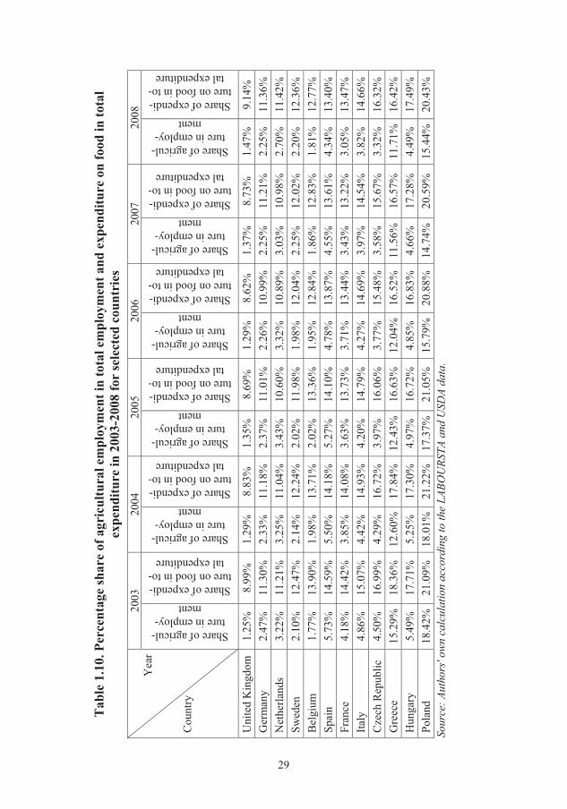
Tab

le 1

.10.

Per

cent

age

shar

e of

agr

icul

tura

l em

ploy

men

t in

tota

l em

ploy

men

t and

exp

endi

ture

on

food

in to

tal

expe

nditu

re in

200

3-20

08 fo

r se

lect

ed c

ount

ries

Yea

r

C

ount

ry

2003

20

04

2005

20

06

2007

20

08

Share of agricul-ture in employ-

ment Share of expendi-ture on food in to-

tal expenditure



tal expenditure



tal expenditure



tal expenditure



tal expenditure



tal expenditure

Uni

ted

Kin

gdom

1.

25%

8.

99%

1.

29%

8.

83%

1.

35%

8.

69%

1.

29%

8.

62%

1.

37%

8.

73%

1.

47%

9.

14%

G

erm

any

2.47

%

11.3

0%

2.33

%

11.1

8%

2.37

%

11.0

1%

2.26

%

10.9

9%

2.25

%

11.2

1%

2.25

%

11.3

6%

Net

herla

nds

3.22

%

11.2

1%

3.25

%

11.0

4%

3.43

%

10.6

0%

3.32

%

10.8

9%

3.03

%

10.9

8%

2.70

%

11.4

2%

Swed

en

2.10

%

12.4

7%

2.14

%

12.2

4%

2.02

%

11.9

8%

1.98

%

12.0

4%

2.25

%

12.0

2%

2.20

%

12.3

6%

Bel

gium

1.

77%

13

.90%

1.

98%

13

.71%

2.

02%

13

.36%

1.

95%

12

.84%

1.

86%

12

.83%

1.

81%

12

.77%

Sp

ain

5.73

%

14.5

9%

5.50

%

14.1

8%

5.27

%

14.1

0%

4.78

%

13.8

7%

4.55

%

13.6

1%

4.34

%

13.4

0%

Fran

ce

4.18

%

14.4

2%

3.85

%

14.0

8%

3.63

%

13.7

3%

3.71

%

13.4

4%

3.43

%

13.2

2%

3.05

%

13.4

7%

Italy

4.

86%

15

.07%

4.

42%

14

.93%

4.

20%

14

.79%

4.

27%

14

.69%

3.

97%

14

.54%

3.

82%

14

.66%

C

zech

Rep

ublic

4.

50%

16

.99%

4.

29%

16

.72%

3.

97%

16

.06%

3.

77%

15

.48%

3.

58%

15

.67%

3.

32%

16

.32%

G

reec

e 15

.29%

18

.36%

12

.60%

17.8

4%

12.4

3%16

.63%

12

.04%

16.5

2%

11.5

6%16

.57%

11

.71%

16.4

2%

Hun

gary

5.

49%

17

.71%

5.

25%

17

.30%

4.

97%

16

.72%

4.

85%

16

.83%

4.

66%

17

.28%

4.

49%

17

.49%

Po

land

18

.42%

21

.09%

18

.01%

21.2

2%

17.3

7%21

.05%

15

.79%

20.8

8%

14.7

4%20

.59%

15

.44%

20.4

3%

Sour

ce: A

utho

rs' o

wn

calc

ulat

ion

acco

rdin

g to

the

LABO

URS

TA a

nd U

SDA

data

.

�

30

Table 1.11. Estimates of the trend function describing the increase in transport (in thousand tons of transported products) of food products for Spain and France

Country Slope Constant R2 Spain 0.079 0.605 0.755 France 0.05 1.018 0.866

Source: Own calculations based on the Eurostat data.

Figure 1.12. Rate of changes calculated for the transport of food products for Spain and France in 1991-2007 (1991=100)

Source: Author’s own compilation based on the Eurostat data.

In light of the foregoing, the growth of the processing sector creates the so-

called "price gap", which is the source of financing activity in the food chain, includ-ing funding of services related to the purchase of agricultural products, storage, pro-cessing and enrichment of value in use, primary, wholesale and secondary trade, dis-tribution, retail trade, advertising, etc. According to D. Dahl, J. H. Hammond it can be assumed that "one of the ways to determine the added value in the processing and trade is to include inputs of production factors used in the processing, transport, trade, taking place between the farm and the consumer, in the payment (return) cate-gories. We would then include such categories as wages, as a return on investment of labour in the processing, trading, transportation, etc.; interest on loan capital and capital factor used in the process; pensions, as fees for use of land and buildings; and profit, as a reward for entrepreneurship and risks. Thus we can adopt the name of market costs associated with the movement of the product from the farm to the con-sumer. Another way to define this gap is the term of return on inputs borne by individ-ual participants in the process of processing, transport and trade, in particular the

31

fees charged by retailers, wholesalers, food industry, transports and others. Hence, one can adopt the name of market fees"25.

The increased role of processing is also reflected in the diversity of values of income and price elasticity of demand for food in comparison to the same ratios calcu-lated for agricultural products26. They are, in fact referred to the two levels of the same agri-food market on the basis of the rolling principle, or one can adopt that they pertain to two separate markets.

In the light of these assumptions, for it is the agri-food processor that determines demand conditions for the agricultural producer. The producer should adapt to these con-ditions. Referring to the terminology used in management sciences, the processor can be classified to the nearest market environment of the producer as the most important busi-ness partner. The processor creates a market for the agricultural producer27.

Agri-food processor is responsible for the demand side on the market of agricul-tural raw materials and the market of inputs associated with the processing of agricul-tural products. He is also responsible for the supply side on the market for food prod-ucts. Thus, a system of relationships is created, which should be in general and partial equilibrium. This system can be written as follows:

� �WR�

S�

S CCCf� ,,� (1.20) � �WR�

DR CCCfR ,,� (1.21) � �WR�

DW CCCfW ,,� (1.22)

where: S�f – function of the supply of food products; D

Rf – function of the demand for agricultural products as raw materials; D

Wf - function of demand for inputs related to the processing of agricultural products; �C – price of food product; RC – price of agri-cultural raw material; WC – price of inputs associated with the processing of agricul-tural raw material.

The agri-food processor, by making decisions regarding the use of inputs, in particular regarding the relationship of raw material and its processing, takes into ac-count not only the level of prices of these mutually substitutable inputs28, but also oth-er factors (quality norms and standards, health requirements, which are included in

25 D. Dahl, J.H. Hammond, Market and Price Analysis, The Agricultural Industries, Minne-apolis, 1982, p. 140. 26 W.W. Cochrane, Farm Prices, Minneapolis, University of Minnesota Press, 1986, p. 63. 27 Ibidem, p. 72. We do not include here the importance of direct markets: agricultural pro-ducer-consumer. 28From the micro-economic point of view, the behaviour of the agri-food processor is recognised in terms of the choice of the producer for maximization of his profit function. Inputs, which he uses in operations are, in addition to agricultural raw materials (agricultural products), also the inputs associated with the processing of agricultural raw materials. We assume that the processor acts rationally and has rational expectations. Thus, in a situation in which he anticipates an in-crease in agricultural prices he will intensify its processing, to obtain the maximum effect from the same individual effort (objective functions). The prices of these inputs, i.e. of agricultural raw material and its processing with a given financial limit are components of the budget constraint, i.e. isocosts. This sets pricing terms for agricultural raw materials.

32

costs associated with the processing of agricultural raw materials). Let us then analyse the choice of the agri-food processors. The objective function of the processor is to maximize profit, expressed by the formula:

� � � �� max, �� WCRCWRgC WR� (1.23)

where: � �WRg , – supply of food products; R – agricultural products (agricultural raw material); W – inputs related to the processing of agricultural raw materials.

Decision variables in this approach are the inputs associated with the processing of agricultural products used by the processor as raw materials and the agricultural products. In the latter case, of course, the most important is the buying price of the ag-ricultural product as a raw material. The processor can maximize the objective func-tion for a given production – the maximum effect from given inputs or minimum in-puts for a given production.

In order to reduce the demand, the processor's decision problem can be shown using conditional optimization. Using the Lagrangian function, it is assumed that the objective function of the processor is to minimize the cost incurred to obtain food product for a given amount of production (demand) thus:

min�� WCRC WR (1.24)

While maintaining the condition: ),( WRf� � (1.25)

Which leads to the Lagrange function:

� � � �),(,, WRf�WCRCWR WR �� (1.26) By solving this problem we can derive equilibrium conditions for the agri-food

processor. Prices (pay) for each input must be equal to their marginal productivities, which is the canon for the producer in terms of competitive balance. Then, only the pro-cessor has endogenous sources of funding, because the assumption that the price of the product of the processor is fixed is implicitly held. It is assumed, therefore, that - partic-ularly in the short term - the prices of agricultural raw materials depend on their margin-al utility for processors. This is also determined by the purchase price of the agricultural producer, i.e. the maximum price the processor can pay to the agricultural producer.

Therefore, as we pointed out, the processor is crucial to the sustainability of growth in the agri-food sector, because by seeking to maximize his objective function he determines the price level of agricultural products produced by the producers, under the assumption that the price of agricultural raw materials is determined by their marginal utility for the processor. It is also the basis for isolating the intermediate demand, which is reported by the agri-food processor for agricultural raw materials and direct (final) demand reported by the consumer.

33

1.3. Agricultural producer

From the above and from the literature it follows that increasing agricultural production “meets inelastic demand, causing a fall in real prices of agricultural prod-ucts. As a result, farmers' incomes are not growing in proportion to the rate of growth of production"29. In fact, this also depends on the growth rate of production efficiency. However, agricultural producers cannot rely "on the increase in prices of products as the source of increase in their income"30. Due to the increasing role of the processors as discussed above, and the recessive nature of the market, agricultural producers who seek to improve their income are forced to use the possibilities in the field of produc-tivity of production factors. This also applies to the labour factor31. The growth models used in agriculture include, in particular, the indicators of labour productivity and productivity of the land. This is also the essence of the developed model in relation to agricultural production and agricultural producer. Development of these values and their empirical illustration are contained in chapter 3.

Considering the agricultural producer, it is assumed that the maximized objec-tive function is his income. The essence of this objective function (income) is reflected best by the difference between the revenue (price multiplied by the volume of produc-tion sold) and the costs of the use of production factors (product of the size of the fac-tors used and their prices). This can be rewritten as follows:

� � max�� LCKCRC LKR (1.27) where: KC – price (pay) of material production factor (capital); KC – price (pay) of labour; K – material factor (production assets, fixed assets, including the land and cur-rent assets, both in quantitative and qualitative terms) ; L – labour factor (number of employees, both in quantitative and qualitative terms).

In competitive equilibrium, it is assumed that the level of price received for the product is constant, and the volume of production, which a (single) producer can sell does not meet demand constraints. However, in sectoral terms, due to the homogene-ous nature of the agricultural product, agricultural producers aggregated in the scale of the whole agriculture, face demand constraints. Then the buying price responds to changes in the volume of production and the resulting supply. Supply growth usually leads to a decrease in buying prices and vice versa. This is also expressed in the condi-tional demand of the developed model.

In terms of the microeconomic approach, if we assume demand restrictions, the decision problem of the agricultural producer can be written in the form of the follow-ing conditional optimization task:

� � min�� LCKC LK (1.28) where:

29 A. Wo, W poszukiwaniu modelu rozwoju polskiego rolnictwa, IAFE-NRI, Warsaw 2004. 30 W. Rembisz, Mikroekonomiczne podstawy wzrostu dochodów producentów rolnych, VIZJA PRESS&IT, Warsaw 2007, p. 26. 31But here, because of the many support programs of the CAP, this pressure on the increase in labour efficiency, as the main source of income, is weakening.

34

),( LKfR � (1.29) where: ),( LKfR � – production function of the agricultural producer.

Analysis of the producer’s situation in microeconomic terms requires considera-tion of the behavioural traits of agricultural producers (farms) for the prices of produc-tion factors (price paid) and produced agricultural products (prices received). Models determining sensitivity of the producer to changes in relative prices are essential in such considerations. In this approach, there is often a need to define the production function describing the production process, which results in the conversion of produc-tion factors into the product32.

32Empirical illustration of the producer’s issue is in this approach often associated with the estimation of parameters of the corresponding functions. In this paper we abandoned this type of modelling which requires the direct application of the production function with a fixed ana-lytical form for several reasons. The first is the disagreement among economists as to the classification of production factors and measuring of their costs. As a manifestation of this absence of an agreement, we can indicate for example a dispute between Cambridge vs. Cam-bridge, originating from the unclear treatment of the capital factor. Moreover, when studying the agricultural sector functioning in a given economy as a whole, without distinguishing be-tween the producers of particular products, there may be significant differences between the factors of production and the analytical forms of production functions. In addition, some of the costs incurred by agricultural producers are in practice difficult to estimate. This applies especially to farmer's own labour or labour of his family, for which they do not receive wages.

35

2. Role of the processor in the growth model of agri-food production

Agricultural producer, as indicated above, operates in conditions shaped by oth-er market participants, i.e. the consumer and the agri-food processor. Influence on the part of the consumer results from the increased demand for processed products, which in turn entails the increasing role of the processor. The increasing importance of the latter is associated with the role of prices of agricultural products, which are used by the processor as raw materials. As indicated above, the agri-food processor seeking to maximize the profit replaces relatively more expensive input by the relatively cheaper one. This has implications for the agricultural producer. The processor, in fact, seeks to use agricultural raw materials in a most rational way in order to maximize profit. He processes them more completely add-ing value in use. This creates demand and limits increase in prices of agricultural products. With a given formula of revenue of the agri-food processor (2.1), we can determine demand for agricultural products and inputs related to their processing:

WCRC�C WR� �� (2.1) The demand for agricultural raw material is as follows:

R

�

C�C

R�

� (2.2)

The demand for other inputs related to the processing, transport and trade in food:

W

�

C�C

W�

� (2.3)

Using (2.2) and keeping the assumption of a constant price level of food prod-ucts ( �C ), we get the following formula:

RR

��

CC

R

R ��

��

� (2.4)

The right side of equation (2.4) is the rate of change in the gap, which reflects the change in the degree of use of agricultural raw materials by the processor. This determines the increase in prices of agricultural products.

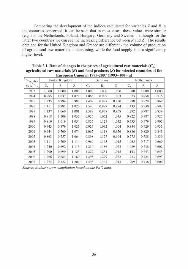
Tables 2.1 and 2.233 illustrate the above considerations concerning the rate of changes by including indexes calculated for the following variables: pork prices to the producer ( RC ), production volume of meat produced by producers (R) and food pro-duction (from pork – �), while Table 2.3 presents estimates of linear trend functions for the respective indices and coefficients of determination. The results lead to the conclusion that the price of raw material ( RC ) increased significantly in Belgium. In turn, the variable R was characterised by a growing trend, inter alia, in Italy, Spain and Germany, and a decreasing trend in Hungary, the Netherlands and the UK. The varia-ble � was characterised by a growing trend in the UK, Germany and Sweden, and a decreasing trend in the Netherlands.

33 In tables 2.2 and 2.5 Belgium is recognised together with Luxembourg.

36

Comparing the development of the indices calculated for variables � and R in the countries concerned, it can be seen that in most cases, these values were similar (e.g. for the Netherlands, Poland, Hungary, Germany and Sweden - although for the latter two countries we can see the increasing difference between R and �). The results obtained for the United Kingdom and Greece are different - the volume of production of agricultural raw materials is decreasing, while the food supply is at a significantly higher level.

Table 2.1. Rate of changes in the prices of agricultural raw materials (CR),

agricultural raw materials (R) and food products (�) for selected countries of the European Union in 1993-2007 (1993=100) (a)

Country Year

United Kingdom Germany Netherlands CR R � CR R � CR R �

1993 1.000 1.000 1.000 1.000 1.000 1.000 1.000 1.000 1.0001994 0.985 1.037 1.028 1.065 0.989 1.003 1.073 0.958 0.7161995 1.235 0.994 0.987 1.408 0.988 0.970 1.298 0.929 0.8681996 1.411 0.981 1.020 1.540 0.997 0.994 1.433 0.930 0.8921997 1.137 1.066 1.001 1.389 0.978 0.968 1.292 0.787 0.8391998 0.818 1.109 1.032 0.926 1.052 1.035 0.822 0.987 0.9251999 0.819 1.019 1.054 0.835 1.125 1.032 0.733 0.979 0.9052000 0.943 0.879 1.023 0.926 1.092 1.004 0.844 0.929 0.9332001 0.944 0.760 1.074 1.067 1.118 0.976 0.886 0.820 0.8432002 0.863 0.757 1.064 0.898 1.127 0.994 0.775 0.788 0.8392003 1.111 0.700 1.114 0.960 1.163 1.015 1.065 0.717 0.6602004 1.240 0.692 1.115 1.210 1.186 1.022 1.089 0.738 0.6022005 1.290 0.690 1.123 1.222 1.234 1.015 1.143 0.743 0.6532006 1.266 0.681 1.180 1.293 1.279 1.022 1.223 0.724 0.6932007 1.274 0.722 1.204 1.493 1.367 1.043 1.209 0.738 0.606

Source: Author’s own compilation based on the FAO data.

37

Table 2.2. Rate of changes in the prices of agricultural raw materials (CR), agricultural raw materials (R) and food products (�) for selected countries of the

European Union in 1993-2007 (1993=100) (b) Country Year

Belgium Spain France CR R � CR R � CR R �

1993 1.000 1.000 1.000 1.000 1.000 1.000 1.000 1.000 1.0001994 1.068 1.018 0.786 1.040 1.017 0.983 1.047 1.041 1.0021995 1.232 1.042 0.742 1.255 1.041 0.996 1.237 1.054 1.0091996 1.350 1.069 0.729 1.351 1.128 1.042 1.322 1.062 1.0011997 1.232 1.032 0.650 1.224 1.150 1.057 1.160 1.091 1.0101998 0.853 1.084 0.631 0.867 1.314 1.204 0.844 1.145 1.0611999 0.691 1.004 0.740 0.761 1.385 1.241 0.760 1.157 1.0802000 1.726 1.054 0.751 0.848 1.391 1.233 0.807 1.137 1.0932001 1.900 1.073 0.761 1.020 1.431 1.248 0.931 1.138 1.0922002 1.622 1.051 0.691 0.832 1.470 1.264 0.767 1.153 1.0562003 1.789 1.037 0.699 0.946 1.527 1.284 0.872 1.150 1.1162004 2.190 1.065 0.660 1.121 1.473 1.173 1.027 1.127 1.0052005 2.208 1.023 0.678 1.151 1.517 1.178 1.057 1.118 1.0362006 2.284 1.010 0.647 0.866 1.549 1.217 1.118 0.989 0.9342007 2.285 1.070 0.683 0.859 1.647 1.293 1.102 0.999 0.951



European Union in 1993-2007 (1993=100) (c) Country Year

Czech Republic Greece Poland CR R � CR R � CR R �

1993 1.000 1.000 1.000 1.000 1.000 1.000 1.000 1.000 1.0001994 1.215 0.765 0.795 0.989 1.005 1.069 1.246 0.883 0.9351995 1.429 0.817 0.849 0.942 1.005 1.338 1.177 1.031 0.9611996 1.441 0.817 0.850 1.010 0.995 1.164 1.233 1.084 0.9811997 1.235 0.754 0.761 0.927 0.980 1.417 1.276 0.994 0.8591998 1.163 0.774 0.799 0.802 0.987 1.309 1.098 1.065 0.9261999 0.972 0.734 0.776 0.720 1.016 1.499 0.845 1.074 0.9702000 1.011 0.677 0.717 0.743 1.038 1.611 0.937 1.011 0.9482001 1.266 0.674 0.706 0.828 1.003 1.698 1.173 0.972 0.9322002 1.128 0.676 0.716 0.683 0.805 1.498 0.968 1.063 0.9532003 1.169 0.669 0.735 0.866 0.816 1.288 0.906 1.151 0.9892004 1.413 0.692 0.803 0.921 0.790 1.279 1.268 1.028 0.9462005 1.553 0.618 0.812 0.985 0.803 1.391 1.306 1.028 0.9442006 1.619 0.583 0.778 1.046 0.797 1.523 1.268 1.102 0.9992007 1.625 0.586 0.796 1.163 0.748 1.383 1.387 1.130 1.011


38


European Union in 1993-2007 (1993=100) (d) Country Year

Hungary Italy Sweden CR R � CR R � CR R �

1993 1.000 1.000 1.000 1.000 1.000 1.000 1.000 1.000 1.0001994 1.145 0.905 0.919 0.959 1.018 0.991 1.014 1.057 1.0391995 1.375 0.86 0.856 1.17 1 0.958 0.984 1.061 1.0891996 1.141 0.997 0.856 1.268 1.048 1.044 0.996 1.095 1.0791997 1.207 0.864 0.81 1.173 1.037 1.029 0.916 1.131 1.1091998 1.088 0.848 0.793 0.959 1.05 1.106 0.683 1.135 1.1611999 0.834 0.931 0.812 0.805 1.094 1.164 0.613 1.118 1.1382000 0.864 0.912 0.793 0.839 1.099 1.176 0.635 0.951 1.0912001 1.194 0.827 0.749 0.997 1.122 1.25 0.665 0.948 1.0752002 1.095 0.863 0.833 0.745 1.141 1.26 0.61 0.975 1.1182003 1.046 0.759 0.712 0.857 1.182 1.281 0.638 0.988 1.1312004 1.332 0.802 0.813 0.913 1.182 1.285 1.485 1.012 1.1532005 1.419 0.675 0.744 1.028 1.126 1.266 1.528 0.945 1.1252006 1.431 0.727 0.785 1.054 1.159 1.325 1.574 0.908 1.1212007 1.459 0.743 0.8 0.984 1.192 1.36 1.957 0.91 1.148


39

��Table 2.5. Estimates of coefficients of the trend function for price changes of ��cultural raw materials (CR), agricultural raw materials (R) and food products (�)

for selected countries of the European Union in 1993-2007 (a) Country Description CR R �

United Kingdom

Slope 0.0119 -0.0315 0.0136 Constant 0.9936 1.1246 0.9588

R2 0.0773 0.7591 0.8482

Germany Slope 0.0052 0.025 0.0027 Constant 1.1073 0.913 0.9849

R2 0.0099 0.8975 0.2648

NetherlandsSlope -0.0015 -0.0204 -0.0211 Constant 1.0706 1.014 0.9668

R2 0.0009 0.694 0.5212

Sweden Slope 0.0493 -0.012 0.0069 Constant 0.6254 1.1114 1.0501

R2 0.2682 0.4611 0.483

Belgium Slope 0.1034 0.0012 -0.012 Constant 0.7348 1.0324 0.8192

R2 0.7236 0.041 0.3591

Spain Slope -0.0147 0.0463 0.0203 Constant 1.127 0.9654 0.9982

R2 0.1369 0.9349 0.6532 Source: Authors' own calculation according to the FAO data.

40

Table 2.6. Estimates of coefficients of the trend function for price changes of agricultural raw materials (CR), agricultural raw materials (R) and food products

(�) for selected countries of the European Union in 1993-2007 (b) Country Description CR R �

France Slope -0.0064 0.0015 -0.001 Constant 1.0543 1.0783 1.0377

R2 0.0275 0.0127 0.0073

Italy Slope -0.0102 0.0143 0.0292 Constant 1.065 0.9824 0.9328

R2 0.1 0.8932 0.9364

Czech Republic

Slope 0.0262 -0.0214 -0.0079 Constant 1.0732 0.8937 0.856

R2 0.2842 0.8037 0.2368

Greece Slope 0.0037 -0.0204 0.0226 Constant 0.8788 1.0824 1.1839

R2 0.0152 0.7103 0.2773

Poland Slope 0.0092 0.0084 0.0023 Constant 1.0653 0.974 0.9387

R2 0.0602 0.3134 0.0725

Hungary Slope 0.0207 -0.0177 -0.0115 Constant 1.0096 0.9891 0.9102 R2 0.2197 0.6953 0.5216

Source: Authors' own calculation according to the FAO data. Maximizing the objective function of the agri-food processor given by the formula

(1.23) and determining its extreme, allows for obtaining expressions determining the level of input prices from the demand side shaped by the processors. This also encompasses the prices of agricultural raw materials ( RC ), the level of which depends on the price of the food product ( �C ). One can observe an increase in the gap between the growth in demand for finished food products and the growth in demand for agricultural products as raw ma-terials for the manufacture of food products. There is also an increase in the gap between the price of agricultural raw material and the price of already processed food product.

Table 2.7 contains estimates of the coefficients of linear trend function (with er-ror estimates) describing changes in the price gap SR calculated according to the for-mula (2.5) for food products in selected countries of the European Union.

R

�R C

CS � (2.5)

It may be noted that in some countries this Figure followed the rising trend. On the basis of a sample drawings 2.1. and 2.2 made for selected countries, it can be concluded that the price gap is not constant. This means that the agri-food processor does not earn

41

the income from the gap at a constant level, at the expense of the agricultural producer to some extent. There are many indications that it absorbs or neutralizes the effects of the natural volatility in prices of agricultural products in relation to the finished food products.

* * * As emphasised in accordance with the principles of sound management, the pro-

cessor must either maximize the utility effect in the form of food goods from purchased raw materials, or minimize the consumption of raw materials for the given utility effect. It comes down to the cost of obtaining unit utility – the food goods. At a given time, the lev-el of isocost straight for the processor mostly results from the price level of agricultural products purchased as food raw materials. This also affects the market-shaped part of the value of agricultural product in the food product. This process is done on the basis of mu-tual influence. In fact, it is the market settlement of conflicting interests of the agricultural producer, as a supplier of raw materials and the interests of agri-food processor, as a pro-ducer of finished food goods. The question is only whether or not, the market where these contradictions are settled has the characteristics of a market with competitive balance. This is the mechanism explaining the decrease in the share of the agricultural producer in the final price of the food goods. This results from the consumer choices. The consumer, maximizing its objective function at increasingly higher income and time restrictions, pre-fers more and more the finished processed food product. We have outlined this in the first chapter. In fact, the consumer selects agri-food processors’ services that are more ad-vanced and more diverse. Thus, it is the consumer who finally accepts or verifies these services, which are financed from the gap between the price of the finished food product and the price of agricultural raw material.

With this in mind, we can show the role of processing in the growth model of agri-food production, starting from the pre-established objective function of the pro-cessor (1,123-1.26), i.e.

),( WRf� � (2.6) After transformations of the function 2.6 according to W. Rembisz we get the following:

wSrS� RRS )1( �� (2.7)

where: � – growth in the supply of food products; RS – share of agriculture in the val-ue of the food product; )1( RS� - share of processing services in the value of the food product; r – rate of growth of agricultural production, w – rate of growth in the supply of services relating to the processing of raw materials and trade in food products.

According to equation 2.7, the rate of growth in the supply of food products is a weighted average of the rate of growth of agricultural production (r ) and the rate of growth in the supply of services related to processing, distribution and consumption (w ). Weights are the discussed share of agricultural raw material in the price of the product or in the supply of food products, or in consumer spending in macro-economic terms. There-fore, the increase in demand for finished food products is not transmitted directly to the increase in demand for agricultural raw materials, and thus the possibility of increasing agricultural production and procurement prices34. From the above it follows that the share 34 W. Rembisz, Mikro- i makroekonomiczne…, op. cit., p. 138.

42

of agricultural income from the final consumer expenditure on food decreases. These are sums counted in billions of consumer spending as a source of income for agricultural pro-ducers, which creates certain political and propaganda friction.

Table 2.7. Estimates of the trend function coefficients for price gap (SR) of food products in selected countries of the European Union in the period

from 01.2005 to 03.2011 (01.2005=100) Country Slope Constant R2

United King-dom

0.0003 0.9951 0.2644 (0.0001) (0.0027)

Germany -0.0001 0.9979 0.0119 (0.0001) (0.0042)

Netherlands -0.0013 0.9997 0.4071 (0.0002) (0.0083)

Sweden -0.0002 0.9942 0.0649 (0.0001) (0.0044)

Belgium 0.0011 0.9960 0.6360 (0.0001) (0.0043)

Spain 0.0002 0.9984 0.0578 (0.0001) (0.0036)

France 0.0009 0.9728 0.2450 (0.0002) (0.0083)

Italy -0.0004 0.9939 0.1031 (0.0001) (0.0057) Czech Republic

0.0014 0.9888 0.7091 (0.0001) (0.0045)

Greece 0.0003 0.9785 0.0881 (0.0001) (0.0051)

Poland 0.0020 0.9804 0.8203 (0.0001) (0.0048) Source: Own calculations based on the Eurostat data.

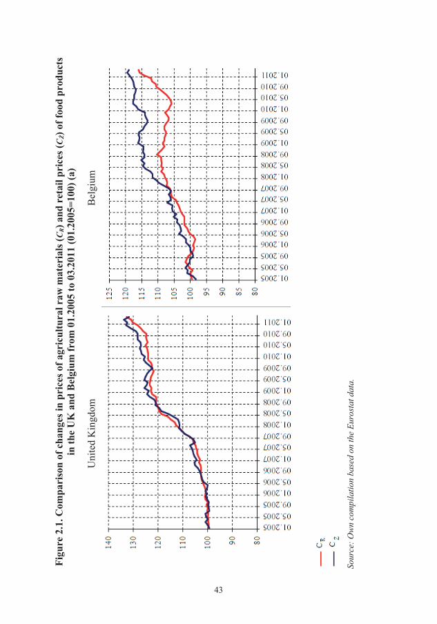
Figu

re 2

.1. C

ompa

riso

n of

cha

nges

in p

rice

s of a

gric

ultu

ral r

aw m

ater

ials

(CR)

and

ret

ail p

rice

s (C

�) o

f foo

d pr

oduc

ts

in th

e U

K a

nd B

elgi

um fr

om 0

1.20

05 to

03.

2011

(01.

2005

=100

) (a)

Uni

ted

Kin

gdom

B

elgi

um

So

urce

: Ow

n co

mpi

latio

n ba

sed

on th

e Eu

rost

at d

ata.

�

Figu

re 2

.2. C

ompa

riso

n of

cha

nges

in p

rice

s of a

gric

ultu

ral r

aw m

ater

ials

(CR)

and

ret

ail p

rice

s (C

�) o

f foo

d pr

oduc

ts

in th

e C

zech

Rep

ublic

and

Pol

and

from

01.

2005

to 0

3.20

11 (0

1.20

05=1

00) (

b)

Cze

ch R

epub

lic

Pola

nd

So

urce

: Ow

n co

mpi

latio

n ba

sed

on th

e Eu

rost

at d

ata.

��

45

3. Growth factors of agricultural production in the developed model

We assume, in accordance with the facts, that the rate of growth of agricultural production (or more accurately the supply of agricultural products) is essential in shap-ing the growth of the supply of food products. This indicator, which is ( r ), is referred to in the developed model of growth in agri-food production. We focus on the rate of growth of agricultural production and the factors that shape this rate.

Analysis of the growth factors of agricultural production can be conducted in macroeconomic or microeconomic perspective, and in the long- and short-term (in economic terms). In the case of microeconomic approach in the short-term (static, be-cause technical changes are not possible) special importance is given to the behaviour-al characteristics of agricultural producers. The above takes into account the variables that directly affect the objective function of the agricultural producer, i.e. prices (re-ceived and paid) as well as regulations and support policy. However, in the macroeco-nomic approach, the main point of the analysis is to determine the effect of changes in the use of production factors and their productivity, i.e. the effect of efficiency of pro-duction on the growth rate of production. This also provides for the impact of individ-ual changes in productivity of labour and capital on the growth of production.

3.1. Changes in agricultural land resources and their productivity

Characteristic primary variables of the agricultural sector, which - intuitively speaking - determine the volume of the production are: the value of the land factor and its productivity. The specificity of the agricultural function of production has been highlighted, inter alia, by Timmer. He writes that "agriculture is the only sector of the national economy, in which land, as the soil, is a key productive factor of production, which is part of its production function"35. Thus, when determining the level of agri-cultural production36, both in the whole country, as well as in individual farms, we adopt the two variables characteristic for this sector, i.e. the area of agricultural land (land element)37 and the average productivity of the agricultural area unit38. This rela-tionship is written as:

QZ

ZRZR �� (3.0)

35 P. Timmer, Getting Process…, op. cit., pp. 81-82. 36 Assuming that final production is equal to the commodity production, i.e. the production intended for the market. 37 Defined by the involved land factor, W. Rembisz, Mikro- i makroekonomiczne…, op. cit., p. 161. 38 This is a unit productivity of the land factor , W. Rembisz, Mikro- i makroekonomiczne…, op. cit., p. 161.

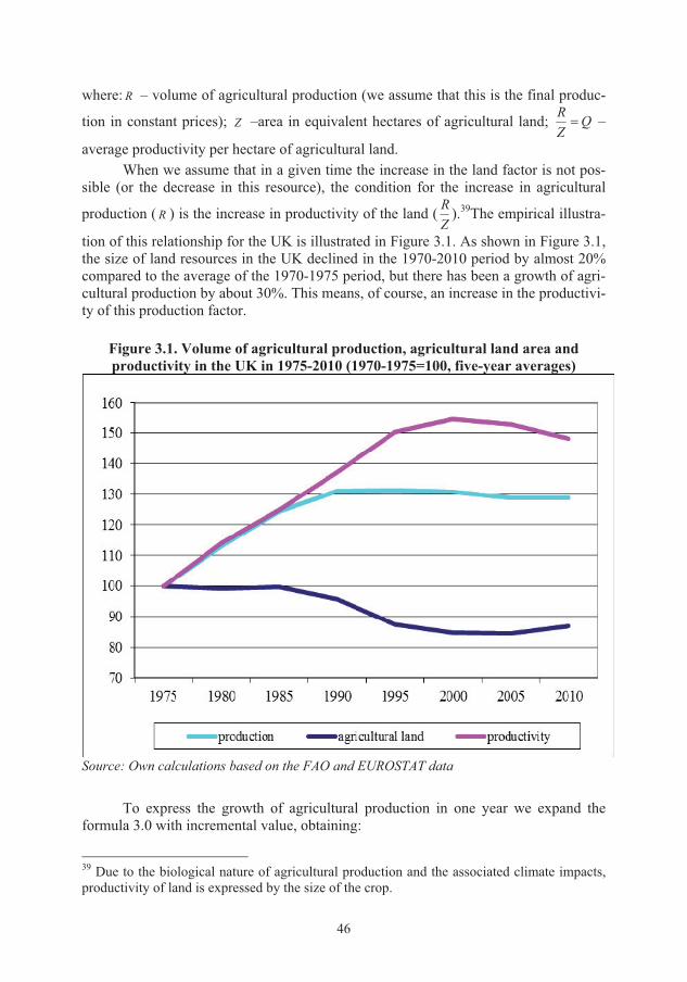
46

where: R – volume of agricultural production (we assume that this is the final produc-

tion in constant prices); Z –area in equivalent hectares of agricultural land; QZR� –

average productivity per hectare of agricultural land. When we assume that in a given time the increase in the land factor is not pos-

sible (or the decrease in this resource), the condition for the increase in agricultural

production ( R ) is the increase in productivity of the land (ZR ).39The empirical illustra-

tion of this relationship for the UK is illustrated in Figure 3.1. As shown in Figure 3.1, the size of land resources in the UK declined in the 1970-2010 period by almost 20% compared to the average of the 1970-1975 period, but there has been a growth of agri-cultural production by about 30%. This means, of course, an increase in the productivi-ty of this production factor.

Figure 3.1. Volume of agricultural production, agricultural land area and productivity in the UK in 1975-2010 (1970-1975=100, five-year averages)

Source: Own calculations based on the FAO and EUROSTAT data

To express the growth of agricultural production in one year we expand the

formula 3.0 with incremental value, obtaining:

39 Due to the biological nature of agricultural production and the associated climate impacts, productivity of land is expressed by the size of the crop.

47

)()( 000 QQZZRR �� (3.1) We obtain the increase in agricultural production in a given year by subtracting

it from the base year ( 000 QZR � ), so we have:

QZQZZQR �� 00 (3.2) Therefore, the growth of agricultural production is determined by three factors:

a. increase in productivity of initial resources of agricultural land ( 0Q Z� � ); b. the effect of changes in agricultural land resource, which achieved the average lev-

el of productivity of the land in the initial period ( 0QZ �� )40; c. product of land productivity gains and changes in the land use ( QZ �� ). This

product approaches zero41. Tables 3.1 to 3.3 present the values of these three factors for selected EU countries. 42Table 3.1 shows the values �f the product 0Q Z� � , Table 3.2 – values of the product 0QZ �� , and Table 3.3 – values of the product QZ �� . Productivity Q

(and its growth Q� ) were measured on the basis of the ratio (ZR ). As shown in Table

3.1, in the majority of the analysed European Union countries the productivity of the land in relation to the resources of agricultural land in 2000 increased in the 2000- -2009 period. The trend can be observed in the case of Poland, Italy and Hungary. The negative value of the product: QZ ��0 was recorded in the case of Greece and the Netherlands. Considerable stability in the productivity of agricultural land resources was observed in Sweden. Table 3.2 presents the value of the product 0QZ �� . On the basis of the data, it can be concluded that in most of the EU countries in the 2000-2009 period there was a reduction in the area of agricultural land43. The strongest effect of reducing the area of agricultural land could be seen in Italy, Greece and Spain. In other countries, we can see a slight variation of this value. The value of the product of the increase in productivity of land and changes in its use ( QZ �� ) was juxtaposed for selected EU countries in Table 3.3. This product demonstrates values close to zero for most countries. The exceptions are countries like Greece, Spain and Italy, which indicates that there were positive effects of the two sources of growth of agricultural production in these countries.

40This ratio can be regarded as an indicator of structural change (growth of farm area) on their production. 41Assuming the loss of land in macroeconomic terms or occurrence of substitution dependence between these values in microeconomic terms. 42 We have chosen the same group of the EU countries, which has been used for the analysis in the previous chapters of the study. 43Where an average level of land productivity was achieved in relation to the initial period (2000).

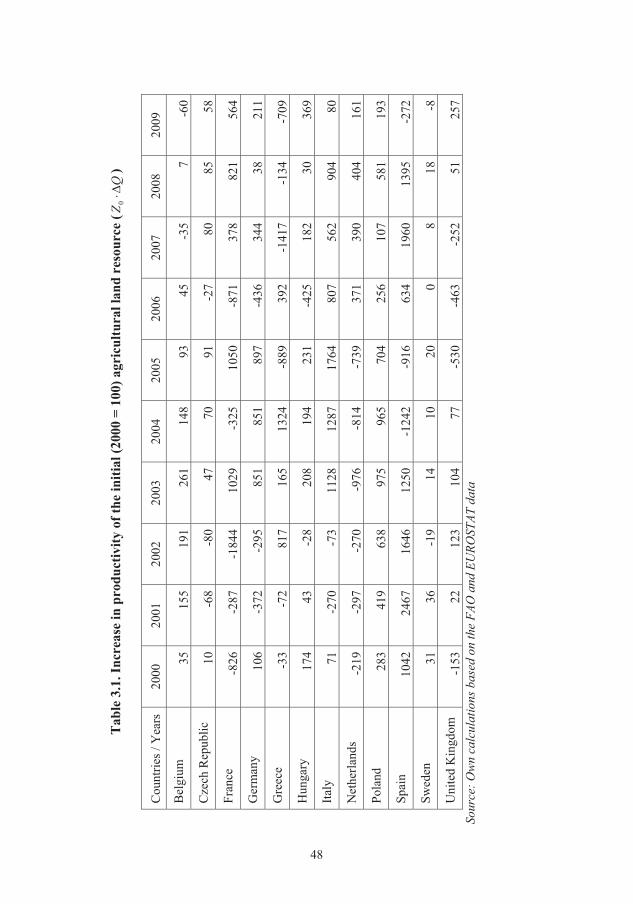
T

able

3.1

. Inc

reas

e in

pro

duct

ivity

of t

he in

itial

(200

0 =

100)

agr

icul

tura

l lan

d re

sour

ce (

QZ

��0

)

Cou

ntrie

s / Y

ears

20

00

2001

20

02

2003

20

04

2005

20

06

2007

20

08

2009

Bel

gium

35

15

519

126

114

8 93

45-3

57

-60

Cze

ch R

epub

lic

10

-68

-80

4770

91

-27

8085

58

Fran

ce

-826

-2

87-1

844

1029

-325

10

50-8

7137

882

156

4 G

erm

any

106

-372

-295

851

851

897

-436

344

3821

1 G

reec

e -3

3 -7

281

716

513

24

-889

392

-141

7-1

34-7

09

Hun

gary

17

4 43

-28

208

194

231

-425

182

3036

9 Ita

ly

71

-270

-73

1128

1287

17

6480

756

290

480

N

ethe

rland

s -2

19

-297

-270

-976

-814

-7

3937

139

040

416

1 Po

land

28

3 41

963

897

596

5 70

425

610

758

119

3 Sp

ain

1042

24

6716

4612

50-1

242

-916

634

1960

1395

-272

Sw

eden

31

36

-19

1410

20

08

18-8

U

nite

d K

ingd

om

-153

22

123

104

77

-530

-463

-252

5125

7 So

urce

: Ow

n ca

lcul

atio

ns b

ased

on

the

FAO

and

EU

ROST

AT d

ata

��

Ta

ble 3

.2. E

ffect

of c

hang

e in

the a

rea

of �

gric

ultu

ral l

and

from

the i

nitia

l (20

00 =

100

) lev

el o

f pro

duct

ivity

of t

he la

nd (

0Q

Z�

�)

Cou

ntrie

s / Y

ears

20

00

2001

20

02

2003

20

04

2005

20

06

2007

20

08

2009

Bel

gium

15

38-6

1-1

125

16

04

-46

Cze

ch R

epub

lic

-4-9

-7-7

-7

-7-7

-7-7

-4

Fran

ce

4994

2015

73

25-3

0-1

94-1

47-9

9 G

erm

any

0-3

123

8511

3 39

-21

2979

62

Gre

ece

-43

-61

-955

-123

-892

74

3-6

9169

5-4

559

9 H

unga

ry

-37

-76

-2-3

-2

0-2

-6-4

-3

Italy

-2

75-4

10-8

27-5

72-8

06

-927

-128

5-5

41-7

89-1

7 N

ethe

rland

s -4

713

-27

1,49

71,

312

1,10

2-4

55-2

99-1

026

Pola

nd

-135

-321

-425

-294

-263

-6

6-3

313

052

16

Spai

n -3

51-5

29-3

66-3

74

-284

-419

-406

-213

-89

Swed

en

-15

-31

-17

-16

8 -7

-8-3

2-8

-4

Uni

ted

Kin

gdom

-2

66-1

42-2

3518

2-6

2 47

128

829

9-4

9-6

3 So

urce

: Ow

n ca

lcul

atio

ns b

ased

on

the

FAO

and

EU

ROST

AT d

ata

�

T

able

3.3

Pro

duct

of t

he in

crea

se in

pro

duct

ivity

of l

and

and

chan

ges i

n ag

ricu

ltura

l are

a (

QZ��

�)

Cou

ntrie

s / Y

ears

20

00

2001

20

02

2003

20

04

2005

20

06

2007

20

08

2009

Bel

gium

0,

1 1,

0-2

,0-0

,50,

6 0,

30,

00,

00,

0-0

,1

Cze

ch R

epub

lic

0,0

0,2

0,2

-0,1

-0,1

-0

,20,

1-0

,2-0

,2-0

,1

Fran

ce

-0,7

-0

,5-0

,60,

3-0

,4

0,4

0,4

-1,2

-2,0

-0,9

G

erm

any

0,0

0,3

-0,2

2,0

2,7

1,0

0,3

0,3

0,1

0,4

Gre

ece

0,1

0,4

-70,

2-1

,8-1

06,1

-5

9,4

-24,

3-8

8,5

0,5

-38,

2 H

unga

ry

-1,3

-0

,60,

0-0

,1-0

,1

0,0

0,2

-0,2

0,0

-0,2

Ita

ly

-0,5

2,

71,

5-1

6,0

-25,

7 -4

0,6

-25,

7-7

,5-1

7,7

0,0

Net

herla

nds

0,6

-0,2

0,4

-79,

6-5

8,2

-44,

4-9

,2-6

,3-2

,20,

1 Po

land

-3

,0

-10,

7-2

1,5

-22,

8-2

0,1

-3,7

-0,7

1,1

2,4

0,2

Spai

n -9

,6

-34,

2-1

5,8

-1,2

-0,1

6,

8-7

,0-2

0,9

-7,8

0,6

Swed

en

-0,1

-0

,30,

1-0

,10,

0 0,

00,

0-0

,10,

00,

0 U

nite

d K

ingd

om

2,2

-0,2

-1,5

1,0

-0,3

-1

3,2

-7,1

-4,0

-0,1

-0,9

So

urce

: Ow

n ca

lcul

atio

ns b

ased

on

the

FAO

and

EU

ROST

AT d

ata

��

51

As is well known due to the increasing competition for land use and urbanisa-tion development of industry, services, etc., which takes place in the European Union, we observe a decrease in the area of agricultural land (in macro-economic terms). 44 These processes imply that the value of the relationship of : 0QZ �� is negative, which is confirmed by the data in Table 3.2. In contrast, as mentioned in the discussion on the formula (3.2), it is different when it comes to the relationship: QZ �� , the value of which is summarized in Table 3.3.

In terms of decrease in agricultural land, which usually refers to the agricultural sector, we have : 0�� QZ and: RZQ �� , and thus increase in the average produc-tivity of agricultural land is higher than the growth of total agricultural production45. Of course, the increase in productivity of the land factor must substitute the effects of the decrease in the land factor. It takes place in a macroeconomic sense, when we are dealing with the real absolute loss of agricultural land46. However, from the microeco-nomic point of view, these expressions mostly have positive values. This follows di-rectly from the concentration processes occurring in farms (expansion of the land fac-tor resource per farm) or in the absence of concentration – substitution by increasing the productivity of the land. However, these relationships in microeconomic terms were not the subject of our interest47.

It can be assumed that in the micro- and macro-economic context the expression 0��Z , therefore, equation (3.2) takes the form:

0ZQR �� (3.3) Interpretation of the formula (3.3) may be that with given resources of the land factor the increase in agricultural production on the farm as well as in the sector is deter-mined by the average productivity of agricultural land.

In addition to the productivity of the land, the factor that also affects the level of agricultural production is the labour factor. The inclusion of labour in growth analysis of agricultural production refers to the classical analysis of economic growth factors. To the equation (3.0) we introduce the level of employment in agriculture, obtaining the relationship: 44 Given the ever-increasing price of land, including arable land, the land is a very attractive means of thesaurisation. However, despite the significant increase in land prices, its supply decreases (due to the obvious fact of resource limitations) with the increasing demand, T. Czekaj, Dochodowo�� materialnych czynników produkcji w gospodarstwach osób fizycznych w 2005 roku, [in:] W. Józwiak (ed.), Sytuacja ekonomiczna i aktywno�� in-westycyjna ró�nych grup gospodarstw rolniczych w Polsce i innych krajach unijnych w latach 2004-2005, Multi-Annual Programme, Report No. 68, IAFE-NRI, Warsaw 2007, p. 61. 45 W. Rembisz, Mikro- i makroekonomiczne…, op. cit., p. 177. 46 In the discussion on the role of the land factor in the potential growth of agricultural pro-duction (defined by the rate of change in arable area and land productivity), one should not forget about the agricultural policy of setting aside land or maintaining it in readiness for pro-duction (fallowing). 47 W. Józwiak, Z. Mirkowska, Ekonomiczne przes�anki zdolno�ci konkurencyjnej polskich gospodarstwa rolnych, [in:] W. Józwiak (ed.), Sytuacja ekonomiczna i aktywno�� in-westycyjna ró�nych grup gospodarstw rolniczych w Polsce i innych krajach unijnych w latach 2004-2005, Multi-Annual Programme, Report No. 68, IAFE-NRI, Warsaw 2007, p. 19.

52

ZR

LZ

LR

�� (3.4)

where: LR – labour productivity per person employed;

LZ – size of agricultural land

per employee; ZR – average productivity of agricultural land.

This equation, also after transformation into a dynamic form, indicates two fac-tors of increase in labour productivity. These are: productivity of the land factor and the amount of land factor per labour factor (the average farm size). It is a formula from the theory of agricultural economics related to Hayami-Ruttan for the developed mod-el of increase in agri-food production. In particular, it shows a simple relationship be-tween the productivity of land and labour productivity. As one can see, labour produc-

tivity (LR ) increases when with a given relationship (

LZ ) the productivity of the land

(ZR ) increases or with the relationship (

ZR ) the area of agricultural land per employee

increases. Table 3.4 shows the resulting values of labour productivity and land produc-tivity in selected countries of the European Union in 2000-2008.

Table 3.4. Average (for 2000-2008) labour productivity, agricultural land

productivity and average size of arable land per person employed in selected countries of the European Union

Country Labour productivity

(LR

)

Productivity of agri-

cultural land (ZR

) Size of agricultural land per employee

Belgium 83 7.45 11 Czech Republic 16 1.00 16 France 66 3.18 21 Germany 41 3.06 13 Greece 18 4.36 4 Hungary 26 1.15 22 Italy 41 5.05 8 Netherlands 73 18.35 4 Poland 6 1.09 5 Spain 45 3.18 14 Sweden 42 1.41 29 United Kingdom 50 3.21 16

Source: Own calculations based on the FAO, EUROSTAT and LABOURSTA data.

3.2. Growth rate of agricultural production

For the needs of the growth of agricultural production as a component of the developed growth model, we divide both sides of the equation (3.2) by equation (3.0). After simplification we get:

53

QZQZ

ZZ

QQ

RR

��

��

��

�� (3.5)

Taking the appropriate symbols to denote growth rates, we have the following

formula (3.5): r q z z q� � � � (3.6)

where: rRR�

� – growth rate of agricultural production48; qQQ�

� – the growth rate of

productivity of land ; zZZ�

� – rate of change of agricultural land resources.

The product of growth rates ( qz � ) due to the substitutability of the processes is close to zero, as already pointed out above, and therefore the equation (3.6) can be re-duced to the following form: 49

qzr �� (3.7) The same result will be achieved by taking logs of the equation (3.6) to the fol-

lowing form: QZR lnlnln �� (3.8)

After differentiating it with respect to time the equation can be written as fol-lows50:

/ / /R t Z t Q t

R Z Q� � � � � �

� � (3.9)

The growth rate of agricultural production (r) is determined by the rate of change of agricultural land and the growth rate of land productivity (q). Conclusions from the equation (3.7) result from the regularity formulated, inter alia, by Hayami and Ruttan, who stated that "the increase in productivity of land has the same effect on the growth of agricultural production as the expansion of crops"51. These issues have been outlined above in general for the equation (3.1). Accordingly, at the macroeco-nomic level, based on the equation (3.7), we can only repeat the previously established observations and regularities, but in dynamic terms. Under normal conditions, the de- 48Some agricultural products are consumed on the spot, i.e. there is natural consumption. In this analysis, we assume that the growth rate of agricultural production ( r ), except for chang-es in inventory, contains an element of the dynamics of change in production for own con-

sumption ( Nr ); 49 Based on W.H. Branson, Macroeconomic theory and policy, 2. Edition, Harper & Row Publishers, New York, 1979. 50Where:

rRR

RtR

��

�� / z

ZZ

ZtZ

��

�� / q

QQ

QtQ

��

�� /

51 Y. Hayami, V. Ruttan, Agricultural Development…, op. cit., p. 310.

54

velopment of agriculture in the EU countries is : 0�z , i.e. the use of land factor in ag-ricultural production is reducing. This is confirmed by the results for selected EU countries (Table 3.5). In most countries, the rate of change of agricultural land re-sources is negative or close to zero (in few cases the value of z was positive). The rate of this loss or the accepted rate of loss of land use factor in agriculture is an economic and regulatory issue52.

It can be assumed that the loss of agricultural land in the economy is inevitable, which can be recognised as:

tzt eZZ 0� (3.10)

where: 10 �� z , is an exogenous variable for the CAP53.

52Causes of reduction in the use of the land factor are known in theory, which we have already pointed out above. Firstly, these are associated in particular with (3.7) and are explained by the analytical model developed in the study. The positive rate: 0q exceeding the effects

0�z is the process of intensification known in the economics. At present "barrier" of de-mand, and in fact the insufficient growth in demand for final agri-food products and for agri-cultural raw materials, there is no need for the two variables included in the equation (3.7) to be positive. Scope of substitution between the two growth factors is quite large, as we show in the formula (3.12). These are somewhat endogenous factors. Secondly, the decline in agricul-tural land resources, or more precisely the agricultural land, is due to the processes of urbani-zation, industrialization, servicisation and development of technical and transport infrastruc-ture and environmental issues. 53 W. Rembisz, Mikro- i makroekonomiczne…, op. cit., p. 169.

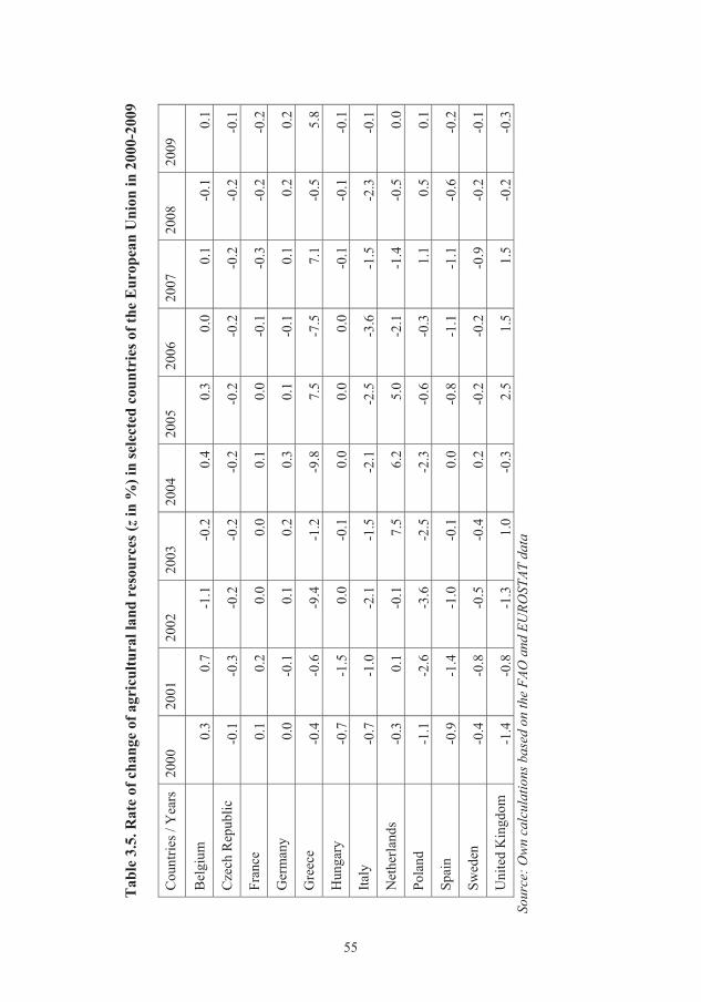
T

able

3.5

. Rat

e of

cha

nge

of a

gric

ultu

ral l

and

reso

urce

s (z i

n %

) in

sele

cted

cou

ntri

es o

f the

Eur

opea

n U

nion

in 2

000-

2009

Cou

ntrie

s / Y

ears

20

00

2001

20

02

2003

20

04

2005

20

06

2007

20

08

2009

Bel

gium

0.

3 0.

7-1

.1-0

.20.

4 0.

30.

00.

1-0

.10.

1 C

zech

Rep

ublic

-0

.1

-0.3

-0.2

-0.2

-0.2

-0

.2-0

.2-0

.2-0

.2-0

.1

Fran

ce

0.1

0.2

0.0

0.0

0.1

0.0

-0.1

-0.3

-0.2

-0.2

G

erm

any

0.0

-0.1

0.1

0.2

0.3

0.1

-0.1

0.1

0.2

0.2

Gre

ece

-0.4

-0

.6-9

.4-1

.2-9

.8

7.5

-7.5

7.1

-0.5

5.8

Hun

gary

-0

.7

-1.5

0.0

-0.1

0.0

0.0

0.0

-0.1

-0.1

-0.1

Ita

ly

-0.7

-1

.0-2

.1-1

.5-2

.1

-2.5

-3.6

-1.5

-2.3

-0.1

N

ethe

rland

s -0

.3

0.1

-0.1

7.5

6.2

5.0

-2.1

-1.4

-0.5

0.0

Pola

nd

-1.1

-2

.6-3

.6-2

.5-2

.3

-0.6

-0.3

1.1

0.5

0.1

Spai

n -0

.9

-1.4

-1.0

-0.1

0.0

-0.8

-1.1

-1.1

-0.6

-0.2

Sw

eden

-0

.4

-0.8

-0.5

-0.4

0.2

-0.2

-0.2

-0.9

-0.2

-0.1

U

nite

d K

ingd

om

-1.4

-0

.8-1

.31.

0-0

.3

2.5

1.5

1.5

-0.2

-0.3

So

urce

: Ow

n ca

lcul

atio

ns b

ased

on

the

FAO

and

EU

ROST

AT d

ata

��

56

With reference to equation (3.7) it can be seen that the condition for the growth of agricultural production, i.e.: 0r , is the presence of a suitable substitution between factors of production growth, i.e. between rates of growth: (q) and (z). In order to illus-trate this and conduct further analyses, Table 3.6 summarizes rates of change of land productivity in the selected countries of the European Union. In the 2000-2009 period most countries had a positive rate of change in the productivity of agricultural re-sources, although in some years there was a noticeable decline in the value. The occur-rence of such a large negative rate of change in productivity of agricultural land, in-cluding in the Netherlands, Greece, the United Kingdom (Table 3.6), may be due to the fact that actions taken under the Common Agricultural Policy are focused on in-struments that increasingly prefer non-agricultural rural development and reducing the intensity of agricultural production in farms.

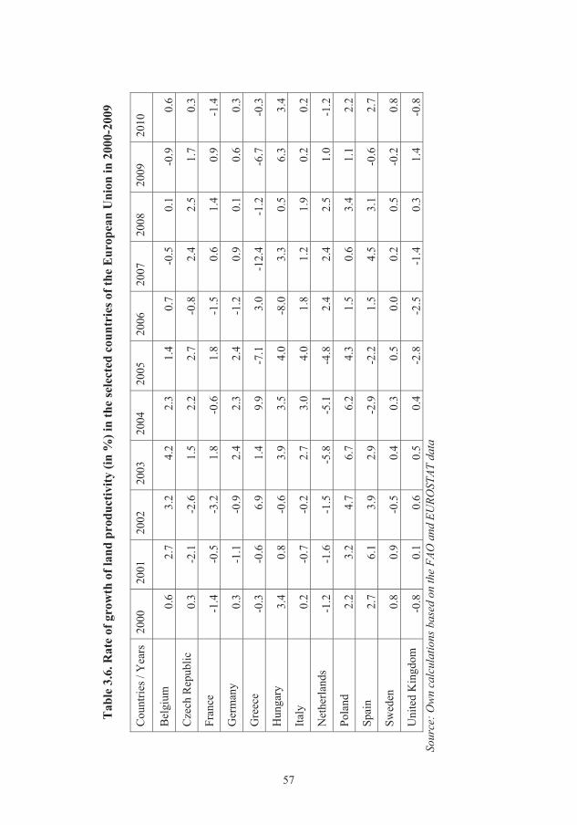
T

able

3.6

. Rat

e of

gro

wth

of l

and

prod

uctiv

ity (i

n %

) in

the

sele

cted

cou

ntri

es o

f the

Eur

opea

n U

nion

in 2

000-

2009

Cou

ntrie

s / Y

ears

20

00

2001

20

02

2003

20

04

2005

20

06

2007

20

08

2009

20

10

Bel

gium

0.

6 2.

73.

24.

22.

31.

4 0.

7-0

.50.

1-0

.90.

6 C

zech

Rep

ublic

0.

3 -2

.1-2

.61.

52.

22.

7 -0

.82.

42.

51.

70.

3 Fr

ance

-1

.4

-0.5

-3.2

1.8

-0.6

1.8

-1.5

0.6

1.4

0.9

-1.4

G

erm

any

0.3

-1.1

-0.9

2.4

2.3

2.4

-1.2

0.9

0.1

0.6

0.3

Gre

ece

-0.3

-0

.66.

91.

49.

9-7

.1

3.0

-12.

4-1

.2-6

.7-0

.3

Hun

gary

3.

4 0.

8-0

.63.

93.

54.

0 -8

.03.

30.

56.

33.

4 Ita

ly

0.2

-0.7

-0.2

2.7

3.0

4.0

1.8

1.2

1.9

0.2

0.2

Net

herla

nds

-1.2

-1

.6-1

.5-5

.8-5

.1-4

.8

2.4

2.4

2.5

1.0

-1.2

Po

land

2.

2 3.

24.

76.

76.

24.

3 1.

50.

63.

41.

12.

2 Sp

ain

2.7

6.1

3.9

2.9

-2.9

-2.2

1.

54.

53.

1-0

.62.

7 Sw

eden

0.

8 0.

9-0

.50.

40.

30.

5 0.

00.

20.

5-0

.20.

8 U

nite

d K

ingd

om

-0.8

0.

10.

60.

50.

4-2

.8

-2.5

-1.4

0.3

1.4

-0.8

So

urce

: Ow

n ca

lcul

atio

ns b

ased

on

the

FAO

and

EU

ROST

AT d

ata

��

58

In macroeconomic terms, in order to achieve a positive growth rate of agricul-tural production (r), it is necessary for (3.7) to meet the following condition:

0� zq (3.11)

At the farm level, but also at the sector level there may be different cases. The

most desirable case appears to be a relationship where both indicators (q) and (r) are

positive, i.e. when there is 0rq . Typically, the demand constraints pertain to (r) as a

macro-economic value, and not (r) as a micro-economic value referring to the farm. This is because the demand conditioning in the agricultural sector scale (macro-economic) is different from that in the scale of a single agricultural producer. These are completely different processes, despite the superficial similarity. Further depend-encies refer to the scale of the agricultural sector. They can, however, also be analysed in the scale of a single producer and his farm, but as regards a different aspect. For an individual agricultural producer (of a farm) there are no restrictions on demand54, equation (3.11) will be satisfied first when two growth factors will be positive, but it is possible to distinguish between:

zq and zq � .

Second, in analytical and accounting terms it is possible, if:

0q and 0�z . but: zq , that is, so that the increase in the productivity of the land substitutes the loss of production effect due to the reduction in the area of agricultural land. Thirdly, where: 0�q and 0z . where zq � , i.e. so that the increase in the size of agricultural resources substitutes for the loss of production due to the effect of reducing the productivity of the land.

Verification of these three cases was carried out by comparing the size of growth rates in Table 3.5 (z) and Table 3.6 (q). Results are shown in Table 3.7. One can see that not all countries in the analysed period had a positive rate of growth (r). This is especially true for Greece and Italy. In Poland, in all analysed years there has been a positive rate of growth of agricultural production. The data in Table 3.7 are characterised by different models of growth of production in agriculture in the light of dependencies contained in (3.4-3.6), which refer to the Hayami-Ruttan approach. 54Of course, in practice, in a given location, with a particular customer, etc., such a restriction exists, but the assumption of competitive conditions is waived in such situation.

T

able

3.7

. Com

pari

son

of q

and

z in

dica

tors

for

sele

cted

EU

cou

ntri

es in

200

0-20

10

C

ount

ries /

Y

ears

20

00

2001

20

02

2003

20

04

2005

20

06

2007

20

08

2009

20

10

Bel

gium

q>

z q>

z 1

1 q>

z q>

z q>

z 0

1 0

q>z

Cze

ch R

epub

lic

1 0

0 1

1 1

0 1

1 1

1

Fran

ce

0 0

0 q>

z 0

q>z

0 1

1 1

0

Ger

man

y q>

z 0

0 q>

z q>

z q>

z 0

q>z

z>q

q>z

q>z

Gre

ece

0 0

0 1

1 1

0 0

0 0

0

Hun

gary

1

0 0

1 1

q>z

0 1

1 1

1

Italy

0

0 0

1 1

1 0

0 0

1 0

Net

herla

nds

0 0

0 1

1 1

1 1

1 q>

z 0

Pola

nd

1 1

1 1

1 1

1 z>

q q>

z q>

z 1

Spai

n 1

1 1

1 0

0 1

1 1

0 1

Swed

en

1 1

0 0

q>z

1 0

0 1

0 1

Uni

ted

Kin

gdom

0

0 0

z>q

1 0

0 1

1 1

0

Val

ue o

f 1 in

dica

tes t

he p

rese

nce

of d

epen

denc

e z

q

or

zq�

whi

ch im

plie

s tha

t r>

0 En

tries

q>

z an

d z>

q o

ccur

whe

n q>

0 a

nd z

> 0,

whi

ch im

plie

s tha

t r>

0 V

alue

of 0

mea

ns th

at n

one

of th

e ab

ove

desc

ribed

cas

es a

re m

et, w

hich

indi

cate

s tha

t r <

0

Sour

ce: O

wn

calc

ulat

ions

bas

ed o

n th

e FA

O a

nd E

URO

STAT

dat

a

�

60

With reference to (3.4) and (3.7) and taking into account the demand condi-tions, it is possible to consider various options for production growth, as well as vari-ous approach to agricultural policy55. To determine the share of indicator (z) and (q) in the rate of growth of production (r), equation (3.1) was transformed. After dividing, we arrive at the following:

rq

rz��1 (3.12)

Relation:rz illustrates the impact of the loss of agricultural land on the rate of

growth of agricultural production. Relation: rq shows the impact of growth of land

productivity on the rate of growth of agricultural production. Note that the relationship

(rq ) expresses the reciprocal of the elasticity of agricultural production towards growth

in land productivity, namely:

RQ

QR

QQ

RR

rq

��

��

��:1

(3.13)

which can also be interpreted as the sensitivity of agricultural production to changes in land productivity.

Figure 3.2 shows the average values of the relationship: (rz ) and (

rq ), designat-

ed for the selected countries of the European Union on the basis of the calculations for the 2000-2009 period. Based on the results listed in Figure 3.2 it can be seen that the changes in agricultural production to a greater extent can be attributed to changes in the land productivity than to the changes in agricultural land resources. The analysis confirms the view expressed in the 1980s by Halcrow that "the growth in agricultural production is increasingly attributable to the growth in yields and animal productivity than to the growth of the agricultural land area”.56 For the majority of the analysed European Union countries the impact of the rate of growth of land productivity on the rate of growth of agricultural production is four times higher than that of the rate of change of agricultural land.

55In terms of demand constraints, there is of course no compulsion to increase land productivi-ty or excessively limit the loss of land resources used in agriculture. It is different, of course, in conditions of demand pressure, as was the case in the centrally planned economy. One should also look differently at these sources of production growth in the conditions of imple-menting the concept of sustainable growth. There must be maintained an appropriate balance between these two sources of growth. We refer to it in further analysis of these formulas. 56 H. Halcrow, Economics of Agriculture, McGraw-Hill, New York, 1980, p. 66.

61

Figure 3.2. Impact of changes in agricultural land resources and land productivity on agricultural production in selected countries of the European

Union - exemplification of the formula (3.18)(Average for 2000-2009)

Source: Own calculations based on the FAO and EUROSTAT data

Having defined the necessary rate of growth of agricultural production resulting from the demand growth, in order to maintain steady growth we can, based on (3.7), determine the necessary rate of growth of land productivity (q):

zrq �� (3.14)

where: *q – desirable - resulting - growth rate of land productivity; *r – desirable (due to market conditions) growth rate of agricultural production; z – rate of changes of agricultural land resources.

The factor which determines the essential rate of growth of land productivity ( �q ), for a given rate of demand for food, is the increasing demand for non-agricultural use of land. Assuming the rate of growth of production ( �r ) conditioned by demand, the necessary rate of growth of land productivity ( �q ) must be higher, the higher is the rate of loss of agricultural land resources57. As mentioned earlier in this chapter, in addition to the land productivity, the factor that also affects the rate of change in agricultural production is the labour productivity (introduced for consideration in equation (3.10). After multiplying (3.10) by the labour factor (L), we arrive at the following:

57At the same time, it should be noted that the rate of land loss can be higher, the greater are the opportunities for increasing rate of land productivity. It is also clear, however, it points to the analytically documented choice, even before the introduction of the policy on the need to intensify agriculture.

62

Z RR LL Z

� � �

(3.15)

After taking the logarithm of the formula (3.21) we have the following: 58

ln ln ln lnZ RR L

L Z� � �

(3.16)

After differentiating formula (3.16) we have the following: 59

/ // // /

Z Rt tR t L t L ZR L Z L R Z

� � � ��

(3.17)

where: rRR

RtR

��

�� /

LrLL

LtL

��

�� / – respectively growth of production and the

rate of change of employment in agriculture ;/

/ Z

Z tL l

Z L

� �� – rate of change in the rela-

tion of the area of agricultural land per employee, which can be expressed as

Z Ll z r� �60;

/

/ /

R Rt QZ Z qR Z R Z Q

� � � �� – growth rate of productivity of agricultural land.

On this basis, equation (3.17) can be written as the following:

qlrr ZL �� (3.18)

Thus, the rate of growth of agricultural production is influenced by: the rate of change in employment, rate of change in area of agricultural land per employee and growth of land productivity. Equation (3.18) combines the elements of the method of growth analysis of agricultural production based on changes in agricultural land resources and their productivity, with elements of analysis based on employment and average labour productivity. Both of these approaches reflect a significant dilemma in economics, what is more important, the increase in labour productivity or increase in land productivity. The correctness of expressions in the formula (3.18) can be easily proved, showing, at the same time, their logic and economic substance. Development of labour and land (concentration ratio illustrating the agrarian structure) can be expressed as the following:

58 Using logarithm properties: ln( ) ln ln lnxyz x y z� � � , for , , 0x y z . 59 Transforming equation (3.21) into (3.23) based on W.H. Branson, Macroeconomic…, op. cit. 60 Based on Sz. Figiel, W. Rembisz, Przes�anki…, op. cit., p. 99.

63

ZL

,

after taking logs61 we have:

ln( ) ln lnZ Z L

L� � , (3.19)

and Z Ll z r� � . (3.20)

What is obvious is the fact that the concentration ratio is the result of changes in the use of agricultural land and changes in employment in agriculture.

With (3.18), we can analyse the impact of the loss of employment and the pro-cess of concentration in agriculture ( 0Zl ) on the rate of growth of agricultural pro-duction. Since we have the following:

rq

rl

rr ZL ��1 (3.21)

The relationship (rrL ) is the impact of the rate of loss of employment on the

growth of agricultural production. Relation (rlZ ) illustrates the impact of increase in

the average area of the concentration process on the rate of agricultural production.

Relationship (rq ) expresses the impact of the increase in land productivity on the rate

of growth of agricultural production. These relationships are also, respectively: rates of flexibility of production growth in relation to employment and the changes in the aver-age area and land productivity.

On the basis of equation (3.14) one can state that the growth of land productivi-ty is a resulting variable defined in the conditions of dynamic equilibrium in the agri-food market for by rate of demand for agricultural products and the rate of land loss. At the same time, (r*) and (z) are influenced by macroeconomic factors, external to agriculture. The first one is conditioned by demand for agricultural products, and the other by demand for non-agricultural land use. Thus, for a relatively steady demand for agricultural products and with decreasing agricultural land resources (Figure 3.1 and Table 3.2 and Table 3.3) to achieve the required volume of agricultural production delineating the balance between the producer and the processor, it is necessary to en-hance the productivity of the land factor. It is obvious that the best source of growth of land productivity is to improve the efficiency of production.

61 (based on the logarithm properties:

ln( ) ln lnx x y

y� � for: , 0x y )

64

Conclusion

In the study we made a preliminary attempt to build a demand conditioned growth model of agri-food production. The model is based on two principles. Firstly, the balancing of the dynamics of demand for agri-food products and agricultural raw materials with the dynamics of their production and supply. Secondly, explanation of the mechanism of behaviours or choices of the main actors in this model, i.e. the con-sumer, the agri-food processor and the agricultural producer, as the most important link in this model. It shows the specificity of demand determinants of increase in agri-food production. In fact, it involves a two-level demand, with two related, but separate markets. The first is the final market of consumer products, agri-food goods. The se-cond market is the market for agricultural products as raw materials for the production of finished food products. In both markets, the elasticity of demand is relatively low and there is a price gap. This creates certain problems when it comes to the implemen-tation of the objective function of agricultural producers. They cannot count on an in-crease in demand and, consequently, an increase in production and prices, as a source of growth of income. This source may be the improved production efficiency. Thus, in the model we emphasize the role and importance of production efficiency by introduc-ing additional explanations and measurement methods, as well as identifications of the sources of improvement.

Developed model allows for analysing different variants of the growth of basic increase in production. These variants are associated with the share of land productivi-ty factor and the changes (loss) as regards application of this factor in agricultural pro-duction to shape its dynamics, as well as in the development of labour productivity, which is also a growth factor. It is a macroeconomic perspective, to which we refer in the model. These figures are illustrated empirically, it was shown that agriculture of the EU countries, which are the subject of the analysis, is dominated by the growth option based on land productivity growth substituting effects of land loss, the loss as-sociated with economic development. Depending on the demand conditions the rela-tionship between the indicator of soil productivity and the effect of its loss are shaped differently. Additionally, we illustrated empirically the impact of changes in labour productivity, in accordance with developed formulas that comprise the model, on the growth of production in relation to other indicators.

The model based on microeconomic analytical formulas describing the choices of the consumer, the processor and the producer has been subjected to a preliminary empirical verification. The data collected from national and international statistics are mainly to illustrate regularities or conclusions derived from the model and the selected analytical formulas. In this sense, empirical analysis and graphical illustrations, as well as specific trend functions of indicators included in the model, verify positively or negatively the assumptions and reasoning. They also entitle to broader observations beyond reasoning tied closely to the model.

Empirical study results show the recessive nature of the agri-food market, which is confirmed by reasoning based on the model, in the sense that its growth rate is continuously decreasing. The rates of the share of food products in consumer spend-ing are decreasing, the structure of consumption is changing to better in terms of

65

health, but to worse from the perspective of agricultural producers, because it does not increase the demand for agricultural raw materials, e.g. as stability and relative decline in the share of meat in consumption and therefore the rate of demand.

Therefore demand can no longer be considered as a growth dynamization factor of agri-food production, at least the domestic demand. This places a greater require-ment for efficiency, both in terms of the agri-food processor and the agricultural pro-ducer. The agri-food processor, maximizing its objective function, makes better use of agricultural raw materials, which relatively reduces the need for increased production of agricultural raw material and the possibility of an increase in its price. We pointed to the potential for improving the efficiency of agricultural producers by providing ownership of the DEA method. On the example of selected countries of the European Union we illustrated the key indicators of the model of growth of agricultural produc-tion and we made a comparison of the indicators between the analysed countries. In order to make generalizations, the development of indicators was aligned to the specif-ic forms of trends.

66

References

1. A European Food Prices Monitoring Tool. A first Design, Luxembourg, October 2009, EUROPEAN COMMISSION, EUROSTAT, Directorate G: Business Sta-tistics, Unit G-6: Price statistics.

2. Banker R.D., Econometric Estimation and Data Envelopment Analysis, Research in Government and Non-profit Accounting, 1989: 5, pp. 231-243.

3. Battese G.E., Broca S.S., Functional Forms of Stochastic Frontier Production Functions and Models for Technical Inefficiency Effects: A Comparative Study for Wheat Farmers in Pakistan, Journal of Productivity Analysis, vol. 1997:8, pp. 395-414.

4. Bezat A., Zastosowanie metody DEA w analizie efektywno�ci przedsi�biorstw rolniczych, Komunikaty, Raporty, Ekspertyzy, No. 545, IAFE-NRI, Warsaw.

5. Bezat A., Jarz�bowski S., Zastosowanie metody DEA w analizie efektywno�ci przedsi�biorstw rolniczych, [in:] B. Barbara Winiowska-Kielian (ed.), Wielokie-runkowo� bada� w rolnictwie i lenictwie, vol. 1, Wydawnictwo Uniwersytetu Rolniczego, Kraków 2008.

6. Boserup E., The Impact of Population Growth on Agricultural Output, Quartely Journal of Economics 1975, No. 2.

7. Branson W.H., Macroeconomic theory and policy, 2. Edition, Harper & Row Publishers, New York 1979.

8. Cervantes-Godoy D,. Dewbre J., Economic Importance of Agriculture for Pov-erty Reduction, OECD Food, Agriculture and Fisheries Working Papers, No. 23, OECD Publishing, 2010.

9. Cochrane W.W., Farm Prices, Minneapolis, University of Minnesota Press, 1986.

10. Coelli T.J., Rao D.S.P., O`Donnell Ch.J., Battese G.E., An introduction to effi-ciency and productivity analysis, 2. Edition, Springer, New York 2005.

11. Cooper W.W., Seiford L.M., Tone K., Data Envelopment Analysis. A Comprehensive Text with Models, Applications, References, 2. Edition, Springer, Berlin 2007.

12. Czekaj T., Dochodowo�� materialnych czynników produkcji w gospodarstwach osób fizycznych w 2005 roku, [in:] W. Józwiak (ed.), Sytuacja ekonomiczna i ak-tywno�� inwestycyjna ró�nych grup gospodarstw rolniczych w Polsce i innych krajach unijnych w latach 2004-2005, Multi-Annual Programme, Report No. 68, IAFE-NRI, Warsaw 2007.

13. Dahl D., Hammond J.H., Market and Price Analysis, The Agricultural Industries, Minneapolis, 1982.

14. Datt G., Ravallion M., How important to India’s poor is the sectoral composition of economic growth?, The World Bank Economic Review 10, 1996, pp. 1-25.

15. Deller S.C., Gould B.W., Jones B., Agriculture and Rural Economic Growth, Journal of Agricultural and Applied Economic, 2003.

67

16. Drummond H.E., Goodwin J.H., Agricultural Economics, Prentice Hall, New York 2011.

17. Figiel Sz., Rembisz W., Przes�anki wzrostu produkcji w sektorze rolno- -spo�ywczym – uj�cie analityczne i empiryczne, Multi-Annual Programme, Re-port No. 169, IAFE-NRI, Warsaw 2009.

18. Fried H.O., Lovell C.A.K., Schmidt S.S., The Measurement of Productive Effi-ciency and Productivity Growth, Oxford University Press, New York 2008, pp. 16-20.

19. Gallup J., Radelet S., Warner A., Economic growth and the income of the poor, CAER Discussion Paper No. 36. Harvard Institute for International Develop-ment: Cambridge, MA, US 1997.

20. Gospodarowicz M., Karwat-Wo�niak B., Zmiany w technikach i organizacji pro-dukcji gospodarstw wysokotowarowych oraz ich wp�yw na kondycj� ekonomicz-n� tych jednostek, Multi-Annual Programme Report No. 159, IAFE-NRI, War-saw 2009.

21. Gospodarowicz M., Procedury analizy i oceny banków, Materia�y i Studia NBP, No. 103, 2000.

22. Halcrow H., Economics of Agriculture. McGraw-Hill, New York 1980. 23. Hayami Y., Ruttan V., Agricultural Development: An International Perspective,

The Johns Hopkins University, Baltimore 1985. 24. Heady E.O., Agricultural policy under economic development, Ames, 1962. 25. Józwiak W., Mirkowska Z., Ekonomiczne przes�anki zdolno�ci konkurencyjnej

polskich gospodarstwa rolnych, [in:] W. Józwiak (ed.), Sytuacja ekonomiczna I aktywno�� inwestycyjna ró�nych grup gospodarstw rolniczych w Polsce i in-nych krajach unijnych w latach 2004-2005, Multi-Annual Programme, Report No. 68, IAFE-NRI, Warsaw 2007.

26. Kaczorowski P., Krajewski P., Mackiewicz M., Piotrowski R., Podstawy ekono-mii matematycznej, PWE, Warsaw 2009.

27. Kreko B., Lehrbuch der linearen Optimierung, Deutscher Verlag der Wissen-schaften, Berlin 1973.

28. Lewandowski J., Zagadnienia rozwoju rolnictwa w socjalizmie, PWE, Warsaw 1972.

29. Mellor J., Ahmed R., Agricultural Price Policy for Developing Countries, The Johns Hopkings University Press, 1988.

30. Meredyk K., Rozwój rolnictwa w warunkach ogranicze popytowych, Zagadnie-nia Ekonomiki Rolnej 1994, No. 3.

31. Rembisz W., Mikroekonomiczne podstawy wzrostu dochodów producentów rol-nych, Vizja Press&IT, Warsaw 2007.

32. Rembisz W., Mikro- i makroekonomiczne podstawy równowagi wzrostu w sektorze rolno-spo�ywczym, Vizja Press&IT, Warsaw 2008.

33. Rembisz W., Analityczne w�a�ciwo�ci funkcji produkcji rolniczej, Komunikaty, Raporty, Ekspertyzy, No. 544, IAFE-NRI, Warsaw 2011, p. 40.

34. Rembisz W., Sielska A., Mikroekonomia – zarys w uj�ciu analitycznym, Wyd. Vizja Press&IT, Warsaw 2011.

35. Riston C. Agricultural Economics Principles and Policy. Westview, Denver, 1992.

36. Senauer B., Major Consumer Trends Affecting the US Food System, University of Minnesota, P-1989-16.

37. Sta�ko S., W�odarczyk M., Ceny detaliczne �ywno�ci a ceny surowców rolni-czych (na przyk�adzie cen skupu pszenicy i cen chleba pszennego), Biuletyn in-formacyjny ARR No. 10, 2006.

38. Thanassoulis E., Introduction to the Theory and Application of Data Envelop-ment Analysis, A Foundation Text with Integrated Software, Kluwer Academic, USA 2001.

39. Timmer P., Getting Process Wright. The Scope and Limit’s of Agricultural Poli-cy, Cornell University Press, Ithaca 1986.

40. Timmer P., The Agricultural Transformation – Handbook of Development Eco-nomics, New York 1987.

41. Tomek W.G., Robinson K.L, Kreowanie cen artyku�ów rolnych, PWN, Warsaw, 2001.

42. Vanderbei R.J., Linear Programming: Foundations and Extensions, International Series in Operations Research & Management Science, Springer 2007.

43. Warr P., Poverty reduction and sectoral growth, results from South East Asia, Australia National University: Canberra, Australia 2001.

44. Wo A., W poszukiwaniu modelu rozwoju polskiego rolnictwa, IAFE-NRI, Warsaw 2004.

45. Yamaguchi Y., Binswanger A., The role of Sectoral Technical Change in Devel-opment. University of Minnesota, pp. 85-7, 1985.

46. Zhang Y., Bartels R., The Effect of Sample Size on the Mean Efficiency in DEA with an Application to Electricity Distribution in Australia, Sweden and New Zealand, Journal of Productivity Analysis. 1998:9, pp. 187-204.

47. Zegar J., Problematyka dochodów ch�opskich, Ubezpieczenia w Rolnictwie. Ma-teria�y i Studia, 3, 1999, pp.7-27.

48. Zió�kowska J., Efektywno�� techniczna w gospodarstwach wielkotowarowych, Studies and monographs, No. 140, IAFE-NRI, Warsaw 2008.

COPY FREE

Print run: 250 copies Printing and binding: EXPOL W oc awek

Growth model of agri-food production - AgEcon...

Documents

Transcript of Growth model of agri-food production - AgEcon...