Growth and redistribution co onents of changes in poverty ...

Journal of Development Economics 38 (1992) 275-295. North-Holland

Growth and redistribution co onents of changes in poverty measures

decomposition with applications to India in the 198Os*

Gaurav Datt and Martin Ravallion

The World Bank, Washington DC, USA

Received August 1940. Sinai version received June I991

We show how changes in poverty measures can be decomposed into growth and redistribution components, and we use the methodology to study poverty in Brazil and India during the 1980s. Redistribution alleviated poverty in India, though growth was quautitatively more important. Improved distribution countervailed the adverse effect of monsoon failure in the late 1980s on rural poverty. However, worsening distribution in Brazil, associated with the macroeconomic shocks of the 198Os, mitigated poverty alleviation through the limited growth that occurred. India’s higher poverty level than Brazil is accountable to India’s lower mean consumption; Brazil’s worse distribution mitigates the cross-country difference in poverty.

1. Introduction

There is often an interest in quantifying the relative contribution of growth versus redistribution to changes in poverty measures. For example, one might want to know whether shifts in income distribution helped or hurt the poor during a period of overall economic contraction. Unfortunately, the numerous existing inequality measures are not particularly useful here. One certainly cannot conclude that a reduction in inequality (by any measure satisfying the usual Pigou-Dalton criterion) will reduce poverty. And even when a specific reduction (increase) in inequality does imply a reduction (increase) in poverty, the change in the inequality measure can be a poor guide to the quantitative impact on poverty. A time series of an inequality

Correspondence to: Poverty Analysis and Policy Division, The World Bank, 1818 street NW, Washington, DC 20433, USA.

*This paper is a product of the World Bank Research Project 67584, and the authors are grateful to the World Bank’s Research Committee for their support. The aper expresses the views of the authors and shoulti not he attributed to ihe World Ban or =ny &hated organization. The authors are grate!ul to the jonrnal’s referees for their comments on an earlier draft. They have also benefited from the comments of Louise Fox, R v Gaiha, Nanak Kakwani. Samuel Morley, George Psacharopoulos, and Dominique van de

0304-3878/92/4iO5.00 ‘(’ 1992~-Elsevier Science

276 G. Datt and M. Ravallion, Changes in poverty measures

measure can be quite uninformative about how changes in distribution have alfected the poor.

This paper shows how changes in poverty measures can be rigorously decomposed into growth and distributional effects, and it illustrates the methodology T::ith recent data for India and Brazil.’

The recent history of poverty in these two countries is of interest from a number of points of view. In Brazil, the 1980s witnessed much lower income growth rates than the 1970s. The effect on poverty of this aggregate stagnation is of particular concern in the light of the widely held belief that inequality in Brazil has also Iworsened in the 1980s. The effects on the poor of the macroeconomic shocks and adjustments of the 1980s in Brazil are of concern. By contrast, reasonable growth rates were sustained in India during the 198Os, and (unlike many developing countries) India survived the period without significant macroeconomic disturbances. However, the mid to late 1980s saw lower Gl?P growth rates overall, due to the low or negative growth rates in agriculture. Monsoon failures were accompanied by con- certed efforts to protect the poor, though we know of no empirical evidence as to whether or not those efforts were successful in avoiding an increase in poverty in the late 198Os, and, if so, what contribution distributional changes made.

The decomposition methodology proposed here is a descriptive tool which can help answer these questions. The following section discusses the decomposition in theory, while section 3 discusses how the theory can be implemented using parameterized poverty measures and Lorenz curves. Section 4 then gives an application to recent data on consumption distributions for rural and urban India. In addition to the substantive issues of interest about poverty in that country, we use these data to investigate a number of more methodological issues of interest about the decomposition. Section 5 gives analogous results for Brazil over a similar period, while section 6 uses the methodology to compare poverty levels between the two countries at one point in time. Some concluding comments are offered in section 7.

2. osition for any c ange in poverty

We confine attention to poverty measures which can be fully characterized in terms of the poverty line, the mean income of the distribution, and the

‘The first application of the method proposed here is Ravallion and Huppi [1989), drawing on results of this paper. A simplified version of our method is used in the f990 World Deueloament Report [World Bank (1990)]. Alternative decomposition techniques ha akwani and Subbarao (1990) and Jain and Tendulkar (1990) on data for 1 a-e are potentially important theoreticai differences between fhese methods and that proposed here, which we will discuss below.

G. Datt and M. Rnraliion, Changes in pocerty measures 277

Lorenz curve representing the structure of relative income inequalities. The poverty flleasure P. =It date (or sk=9innlcnimtrv12 t is written as I -- ---- *-- --c --__, _- -____, ,

where z is the poverty line, p, is the mean income and L, is a vector of parameters fully describing the -Lorenz curve at date t. (Homogeneity in z and p is a common property of poverty measures.) The level of poverty may change due to a change in the mean income pL, relative to the poverty line, or due to a change in relative inequalities L,. For now we can delay discussion of the poverty measure’s precise functional form, or of the Lorenz curve’s parameterization.

The growth componertt of a change in the poverty measure is defined as the change in poverty due to a change in the mean while holding the Lorenz curve constant at some reference level L,. The redistribution component is the change in poverty due to a change in the Lorenz curve while keeping the mean income constant at the reference level p,. A change in poverty over dates c and t + n (say) can then be decomposed as follows:

P ,+n-P,=G(t,t+n;r)+D(t,t+n;r)+R(t,t+n;r) growth redistribution residtxl

component component

in which the growth and redistribution components are given by

while R( ) in (2) denotes the residual. In each case, the first two arguments i

the parentheses refer to the initial and terminal dates of t per-rod, and the last argument makes e to which the observed change

The residual in (2) exists w separable between p and L, i.e., w index of chang curve (mean).

is exposition ur‘ shall c hne.

omposition cl;n also Vf3-t~

measures between countries or regions.

278 G. Dart and M. Ravallion, Changes in poverty measures

apportioned between the growth and redistribution components, as some recent attempts at poverty decomposition have sought to do. For example, Makwani and Subbarao (1990) present results of a decomposition of poverty measures over time for India into ‘growth’ and ‘ineqaality’ components in which the latter is determined as the difference between the actual change in poverty and the growth component. The residual is thus allocated to the redistribution component. This is entirely arbitrary, and also gives the false impression that the decomposition is exact. Similarly, Jain arnd Tendulkar (1990) make the residual appear to vanish by not using consistent reference dates for evaluating the ‘grolnth’ and ‘distribution’ components. In effect, this also amounts to arbitrari!y allocating the residual to either the redistribution or the growth component, though which one depends on the reference dates chosen. Of course, the main issue here is not that the residual must always be separately calculated, but that the growth and redistribution corn must be evaluated consistently.

However. the residual _ ’ itsdf does have an interpretation. To see this, it is instructive to note that, for r=t, the residual in (2) can be written

R(t. t +n; t) =G(t, t +n; r +- nb -G(r, t+n; t)

=D(E,t-5n;t+n)-_(t,t+tl;t). (3

The residual can thus be interpreted as the difference between the growth (redistibution) components evaluated at the terminal and initial Lorenz curves (mean incomes), respectively. lf the mean income cw the Lorenz curve remains unchanged over the decomposition period, then the residual vanishes.3

Separability of the poverty measure between the r~ean and Lorenz parameters is also required for the decomposition to be indc~cndcn~ of the choice of the reference &,I&). That choice is arbitrary; the reference point need not even be historically observed. The initial date of the decorn~Q~~ti~n period is a natural choice of a reference, and this is what we use in the empirical work.

Since it is arbitrary, we shal”, also investigate the sensitivity of the decomposition to the choice of reference. For that purpose, the result in (3) is useful. It tells us that the residual using date t as the reference also gives the change in both the growth component and the redistrib~ti~~ co onent which would result from switching the reference to date tfn. The decomposition using the initial year as the reference contains all the information

‘Note that R(t,t+n;t)= - I R t, t + n; t + n). Thus it is also possible to ma ply averaging the components obtained using the initial and final years as

G. Dart and M. Rarallion, Changes in pwerty ~US~P’QS 279

necessary to calculate the decomposition using the final year as the reference, and vice versa.

The decomposition can also be applied to multiple periods (more than two dates), though a word of caution is needed. A desirable property for such a decomposition scheme is that the growth, redistribution and residual components for the sub-periods add up to those for the period as a whole. However. this property will not hold in general if we use the ~~~tia~ date of each sub-period as the reference. The problem is easily recti that the violation occurs because the reference fp, L) ke sub-periods. The remedy is to maintain a fixed r date for al% decomposition periods. and again the initial date of t ccorn~os~t~o~ period is a natural choice. Sub- itivity is then satisfied. Suppose we have another sub-period fro ate t +H to t+M+k. say. in a dition to the one from f to t + 11 considered above. Then:

G( I, t -I- E: r) + G( t + n. t + n + k; r) = G( L t + !I + k: r),

R( c. c -I- n; r) -I- R(t -I- n. f f n t k; t-1 =

as required for sub-period additivity.’ The interpretation of the residual in the multi-period context is similar to

that for a single decomposition period. For a sequence of dates (0, 1.. . . t, . . . T). let R, denote the residual Rlt - 1. t: 0). The analogue to (3) can then be written in terms of cumulative components:

i R, = R(0, 7-i 0) = G(0, T; T) - GfO, 7: 0) t=l

= NO, T; 7-) - D( 0, T; 0).

e cumulative residual measures the c growth and redistribution components t

reference from date 0 to date 1

3. tis eteriz

The d~com~osit~o~ can

overty dec@??,p0siti0n5 proposed l-q akv%2ni and Subbarao S1990) and Jain and Tendulkar (1990) do no1 satisfy sub-period additivity.

280 G. Datt and M. Rat:allion, Changes in pocertp measures

income or consumption distributions for two or more dates. Explicit functional forms for P(z/~,, f,,,) are derivable for a wide range of existing poverty measures and parameterize Lorenz curves. We shall use three common poverty measures, the headcount index W given by the proportion of the population who are poor, the poverty gap index PG given by the aggregate income short-fall of the poor as a proportion of the poverty line and normalized by population size, and the Foster-Greer-Thorbecke (FGT) PZ measure, similar to PG but based on the sum of squared proportionate poverty deficits. In fact each of these measures is a member of the FGT class of measures P, defined by

where pi is the income or consumption of the ith household or individual, z is the poverty iine, n is the population si?e, and 01 is a non-negative parameter. H is obtained when Q =O; PG is obtained when E = 1; P2 is obtained when r=2.

From any valid parameterized Lorenz curve L(p), H is caiculatable using the well-known fact that $,‘(H)=z. [Noting that a,‘(p) i$ invertible - either explicitly or numerically - for any valid Lorenz curve.] The poverty gap index is then calculated as PG=( 1 -$‘/z)H, where $‘=$,(H)/H denotes the mean income or consumption of the poor. P, is obtained as the integral of [ 1 -(,u/z)L’(y)]’ over the interval (0, H).

We have derived formulae for the FGT poverty measures for each of two parametric specifications of the Lorenz curve, namely the eta model of Kakwani (1980) and the genera1 quadratic (GQ) mode1 of Villasenor and Arnold (1953). Table 1 gives the functional forms of these Lorenz curves, and the implied poverty measures. The derivations of PZ use standard methods of integratiorr. The GQ model gives somewhat easier computational formulae (generating explicit forms for all poverty measures; the Beta specificatio

rical methods for inverting L’(H) and tabulations of incomplete ). Subject to consistency with the theoretical conditions for a

orenz curve, the choice of Lorenz curve specification was made odness of fit. ’ The estimated Lorenz curves for both in the following sections tracked the data extremely we

squares ranged between 0.995 and 1.000 for the two functional forms. (Sue values of are 3re not uncom ese functional for

e also tried a non-linear maximum likelihood estimator of the elliptical model 1983, btit found that this gave almosi identical results to O&S on t

overty measures were within 0.1 prrccnt of

Tab

le

1

Pove

rty

mea

sure

s fo

r al

tern

ativ

e pa

ram

eter

izat

ions

of

the

L

oren

z cu

rve.

Bet

a L

oren

z cu

rve

GQ

L

oren

z cu

rve

- --

_--

-

-.

Equ

atio

n of

the

L

oren

z cu

rve

(UP)

)

Piea

dcou

nt

inde

x

(H)

eHy(

1

_ H

)d [H

i%]=

~ 1.

_

Pove

rty

gap

inde

x (P

C)

PC=

H-(p/z)LJH)

41

-L)=

a(p2

-L)+

bfJp

- I)

+c(p

-L.)

or

, L.

(p)=

-[

bp

+e+

(mp

2+n

p+

e2)“

2]/2

k/J -1

H=

-~

n+r(

b+2Z

/~)(

(b+

2Z/~

)2-m

m)-

“2]/(

2m)

PG=H-(p/z)L(H)

Fost

er-G

reer

-Tho

rbec

ke

( P2)

P2

=(1

-p/z

)[2P

G-(

1 -p/z)H]

P2=

2PG

-H-(

~2/z

2)[u

H+

bL(H

) +B2(p2/z2)[y2B(H,2y-

1,26

+1)

-(

W)l

n ((

1 -H

/Ml

-W2)

)l

-2y~

U?(

H,2

y,26

)+6~

B(H

,2y+

1,25

-1)]

aII(

k,r5

~)=

_ppr

-1(1

-P

)“-‘

dp;

e=

--(a

+h+

c+

1); m

=b2

-44a

; n=

2be-

4c;

r=(n

2-4m

e2)‘

j2;

s, =

(r-n

)/(2

m);

s2

=

-(r+

n)/@

m).

282 G. Da?? and M. Racallion, Changes in perry measures

Lorenz curves.) Imprecision associated with the Lorenz curve estimatir\r. seems unlikely to be of serious con~ern.~

overly in ie, 197749

We have estimated poverty measures and their decompositions for and urban India from the National Sam 1983, 19864987, and 11988. There are a nu across these surveys. The following Iloinis

(ij Doubts have been raised ubout the 1977-1978 survey est expenditures on consumer dtirables, which greatly exceeded esti other years, particularly in rural areas.’ The proble is most serious ~i;i high consumption Bevels, and so may not have much effect on poverty measures. However, the associated distortions in the fitted Lorenz curve could still have a significant effect on the decomposition. (ii) The 1988 distribution is based on a sample which only covered the last six months of that year, while the rest are for a full year. (The survey was also done in the first half of 1989, bu; the results are not yet available.) (iii) The 1986-1987 and 1988 sample were much smaller than those for the other years. 25,800 households were sampled in 1986-1987 and 12, in 1988 (half year) versus 157,900 and 117,9(K) in 1977-1978 and 1983, respectively.’ But they still appear to be large enough to give adequate precision.g

We are able to take corrective action only with regard to (il. Results for a11 years are reported here for both total consumption expenditure, and

%.hl the suggest; &on of a referee, we looked into the possibility of obtaining the standard errors of the decompositions, but this seemed intractable. The problem is two-fold. First, one cannot dismiss the possibility that disturbance terms associated with Lorenz functions may be distributed non-spherically. This does not pose a problem for the estimation of the poverty measures (and hence the decompositions) as the QLS estimates of the Lorenz parameters arc still unbiased, but it does create a problem for the estimation of the standard errors of the poverty measures. Second, while the poverty measures are a function of the Lorenz parameters as we!! as the mean income, the estimates of the Lorenz parameters are constructed differently to that for mean income. The former are estimated econometrically while a sample estimate of the latter is taken directly from published reports. In this context, it is not obvious how the sampling distribution of the poverty measure can be delined.

‘For further discussion see Jain and Tendulkar (1989). 8Sma!!er samples are now being collected on an annual basis, together with the larger samples

at five yearly intervals. Results for the full sample of 1967-1988 were not available at the time of writing.

‘For a random sample, the standard error of the headcount index can be readily calculated using wei!-known results on the sampling distribution of proportions; the standard error of the headcount index H is J[H( 1 - H)/N] where A-V’ is &e sample size. The standard error for the smallest rural (urban) sample (1988) is 1.5 percent (1.9 percent) of our estimate index; for 1986-1987 the correspondin: figure is 1.0 percent (1.3 percent), while fo earlier years it is less that 0.5 percent (0.6 percent).

initial year was usd as the re mer afl dates t

durables makes far more difference ts

ase in the headcount index in kal areas ween 19$~~9$7 owever, the incre is small, and (&vi;n the

in the latter two surveys) it is probabiy not significant statisticaIIy at a reasonable level. 1 ’ Both the poverty gap index and the theoret~~a~~y preferred P2 declined over all sub-periods in rural areas. The pattern is similar for urban areas. There was a particularIy sharp fail in rural poverty 1983 and 19861987.

The comparison of poverty measures across sectors is also of interest. Historically, poverty lines adjusted for cost of living differences have shown higher poverty measures in rural areas than in urban areas, and this is

“Jain and Tendulkar (1989) attempt to deal with this problem by revising the NSS data. have not done so here for two reasons: (i) the best way of making such revisions is quite unclear, and (ii) in any case it could reasonabty be argued that consumption net of durables 1s a tter indicator of living standards for poverty measurement.

“These are perhaps not ideal as for instance ar Minhas et al. (1987, 1988) who als as their indices end and their data are unavailable we have period of our analysis. (We note some r

12We ignore spatial price diNerentials. Elsewhere we differentials in poverty asessme state level estimates [Datt and are very similar to those estim

13Using the usual formula for the standard error of the diBerence proportions,

se(H, -N,)=\4[H,(

one fmds that [H, -H2]/se(M,

though the durablts estimates for these i


Table 2

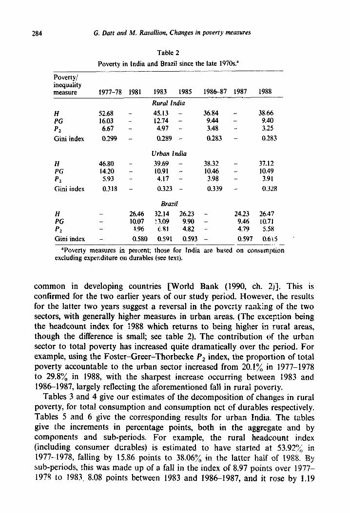
Poverty in India and Brazil since the late 1970s.

Poverty/ inequality measure 1977-78 1981 1983 1985 198687 1987 1988

H 52.68 PG 16.03 p2 6.67

Gini index 0.299

H 46.80 - 39.69 - 38.32 37.12 PG 14.20 10.91 - 10.46 10.49 P, 5.93 ._ 4.17 - 3.98 3.91

Gini index 0.318 - 0.323 - 0.339 0.328

H PG p2

Gini index

- - -

Rural India

45.13 - 12.74 - 4.97 -

0.289 -

36.84 38.66 9.44 9.40 3.48 3.25

0.283 0.283

Urban lndia

Brad

26.46 32.14 26.23 - 10.07 ! 3.09 9.90 - A.96 C.81 4.82 -

0.580 0.591 0.593 -

24.23 26.47 9.46 IO.71 4.79 5.58

0.597 0.6 15 *

aPoverty measures in percent; those for India are based on consumption excluding expenditure on durables (see textj.

common in developing countries [World Bank (1990, ch. 2):. This is confirmed for the two earlier years of our study period. However, the results for the latter two years suggest a reversal in the poverty ranking of the two sectors, with generally higher measures in urban areas. (The exceF:ion being the headcount index for 1988 which returns to being higher ig rural areas, though the difference is small; see table 2). The contribution of the urban sector to total poverty has increased quite dramatically over the period. For example, using the Foster-Greer-Thorbecke P2 index, the proportion of total poverty accountable to the urban sector increased from 20.1% in 1977-1978 to 29.8% in 1988, with the sharpest increase occurring between 1983 and 1986-1987, largely reflecting the aforementioned fall in rural poverty.

Tables 3 and 4 give our estimates of the decomposition of changes in rural poverty, for total consumption and consumption net of durables respectively. Tables 5 and 6 give the corresponding results for urban India. The tables give the increments in percentage points, both in the aggregate and by components and sub-periods. For example, the rural headcount index (including consumer dr;rables) is estimated to have start 1977-1978, falling by 15.84 points to 38.06% in t

sub-periods, this was made up of a fall in the inde 1978 to 1983, 8.08 points between 1983 and 1986-1987, and it rose by 1.19

Period

1977-78 to 83 1983 to 86-87 198687 to 88

1977-78 to 88

1977-78 to 83 1983 to 86-87 1986-87 to 88

1977-78 to 88

1977-7& to 83 1983 to &C&7 19&C&7 to 88

1977-78 to 88

G. Datr and .%I. Racallion. Changes in pocerty measures

Tabk 3

Decompositions for rural India (including consumer durablesl.

Growth Redistribution componenta componenta Residual”

Headcount index (H)

- 2.58 -6.51 0.12

- 8.61 0.19 0.34

1.46 0.27 -0.54

- 9.74 - 6.05 - 0.07

Poverty gap index 1 PG)

- 1.18 -2.09 0.14 - x52 -0.18 0.42

0.55 - 0.54 -0.14

-4.14 -2.81 0.41

Foster-Greer- Thorhecke index 4 P,)

-0.57 - 0.90 0.08

- 1.61 -0.11 0.23

0.24 - 0.46 - 0.04

- 1.94 - 1.47 0.30 -.-. -___

- 11.97

- 8.88

1.19

- 15.86

-3.13

- 3.28

-0.13

-6.54

- 1.39

- 1.49

- 0.26

-3-11

“Percentage points.

Table 4

Decornpczition; ;‘or A.VZ! !ndia (excluding consumer durables).

Period .__

1977-7s to 83 1983 to 136-87 198fvE7 to 8X

1977-78 to 88

Growth Redistribution Total change componenta componenta Residual” in poverQa

--- Headcount index (H)

- 6.45 - 1.18 0.09 - 7.54 - 7.33 - 0.72 - 0.24 - 8.29

1.04 1.44 - 0.66 1.82

- 12.74 - 0.46 -0.82 - 143x

1977-78 to 83 1983 to &6-R7 1986-87 to &R

1977-78 to 8X

- 2.82 - 2.87

0.39

-5.3

Pt)i’rrtr gap inde.y (PG)

- 0.53 0.06 - 3.“9 - 0.54 0.1 I - 3.369 -0.19 - 0.24 -0.04

- 1.24 - O.cBf - 6.63

Foster-Grerr-~Phorhrh,ke index C P2 i

1977-78 to 83 - 1.40 -0.34 I) - I.7 19x3 to 86-87 - I .34 -0.X 0.13 - n.49 1986-87 to X8 0.17 - 0.37 - 0.03 - 0.23

1977-78 10 X8 ---‘.%i - 0.w 0 i! _~ 3.32

“Percentage poinls.


Period

Table 5

Decompositions for urban India (including consumer durables).

Growth Redistribution Total change- componenta componen ta Residual” in povertya

1977-78 to 83 -3.15 1983 to 8687 -4.41 1986-87 to 88 --0.36

1977-78 to 88 - 7.92

1977-78 to 83 1983 to 86-87 1986-87 to 88

197?-78 to 88

1977-78 to 83 1983 to 8687 1986-87 to 88

1977-78 to 88

Headcount index (H)

- 1.30 -0.04 3.02 0.03

- 1.91 1.01

-0.18 0.98

- 1.33 - 1.75 -0.14

- 3.22

Poverty gap index (PC)

-0.96 0.02 1.48 -0.16

- 0.05 0.15

0.46 0.02

Foster-Greer-Thorbecke index (P2)

-0.65 - 0.65 0.03 -0.83 0.76 -0.11 - 0.06 - 0.02 - 0.02

- 1.55 0.09 -0.09

- 4.49 - 1.36 - 1.26

-7.12

- 2.27 - 0.43 -0.04

- 2.74

- 1.27 -0.18 -0.10

- 1.55

aPercentage points.

Table 6

Decompositions for urban India (excluding consumer durables).

Period --_

1977-78 to 83 1983 to 86-87 198687 to 88

1977-78 to 85

Growth Redistribution Total change componenta componenta Residual” in povertya

_-- ._._ Headcount index (f-i)

- 8.35 1.26 - 0.03 -7.12 - 3.26 1.79 0.10 - 1.37 - 0.79 - 1.95 1.54 - 1.20

- 12.41 1.11 1.62 -9.68

!977-78 to X3 1983 to X6-87 1986-87 to 88

1977-78 to 88

- 3.47 - 1.24 - 0.29

- 5.00

Poverty gap index (PC)

0.30 -0.12 - 3.29 0.99 - 0.20 -0.45 0.10 0.22 0.03

1.39 -0.10 -3.71

Foster-Greer-Thorbecke index ( Pz)

1977-79 tc 83 - 1.69 -0.01 - 0.06 - 1.76 1983 to rib-87 -0.57 0.55 -0.17 -0.19 1986-87 to 88 -0.13 0.13 - 0.07 - 0.07

1977-78 to 88 - 2.40 0.67 -0.29 - 2.02


G. hiii mid h‘. Ravaiiion, Changes in gocerty measures 287

points between 19861987 and 1988. By components, distributionally neutral growth accounted for 9.74 points, distributional shifts accounted for 6.05 points, with the residual making up the balance of O.Q? points.

A number of points are noteworthy from the results of tables 3 and 4:

(i) The adjustment for durables makes considerable difference to the decompositions, particularly for the period 1977-1978 to 1983. When durables are included. the redistribution component dominates the growth component for all poverty measures. However, the ranking is fully reversed when durables are excluded (table 4). The growth component now dominates for all measures. As doubts can be raised about the 1977-1978 durables expenditures in the NSS, we suspect the results of table 4 to be closer to the truth, and we will confine our attention to those results in the following discussion. (ii) While the growth component dominates the redistribution component in all sub-periods, the relative importance of the two can vary greatij* azcordang to which measure of poverty is used. This is most striking for the last period, 1986-1987 to 5988. For the headcount index we find that both the growth and redistribution components contributed to the increase in poverty.

wever, for the other two measures, changes in distribution mitigated the erse effect of the decrease in the mean. Roughly speaking, people with

consumption around the poverty line became worse off over this sub-period, while the poorest became better off. However, the problems of comparabihty between these NSS rounds should be retailed, though we do not know what direction of bias, if any, may be attributed to those probleLls. (iii) The residuals in the decomposition vary a good deal in size. Our results suggest it would be hazardous to assume the residual is zero, or simply lump it into the redistribution component. For example, for the headcount index (excluding durables) over the whole period, 1977-1978 to 1988, the residual exceeds the redistribution component (in absolute value), and by a margin. However, in all other cases the residual is small relative to growth and redistribution components. Thus the decomposi!ion is generahy quite insensitive to a change of reference from the initial to final year. {Usi the results of section 2, the changes invo making such a Gtcb whole period can be obtained easily fro es 3 and 4 by si the residual to the growth and redistrib~~t~Q~ corn the final year as the refcre residual for the initial year).

288 G. Dart and M. Racallion, Changes in poverty measures

the headcount index and the Foster-Greer-Thorbecke P, measure, albeit in opposite directions (table 4). (v) The rather sharp fall in rural poverty over the whole period, particularly between 1983 and 1986-1987, warrants further comment. 1986-1987 was not a good agricultural year; indeed, it was a bad one in much of Western India, with below normal rainfall and a decline in output. It is arguable that the CPIAL may have under-estimated the rate of inflation; the CPIAL increased by 13 percent over this period while wholesale prices increased by 19 percent. Similar concerns about the use of CPIAL as a deflator for th- period 1973- 1974 to 1983 have been expressed by Minhas et al. (1987). The poverty measures are quite sensitive !c, changes/measurement errors in the deflator. For instance, an under-estimation of inflation over the period 1983 to 19f%- 1987 by 1 percent would result in underestimating the headcount, the poverty gap, and the Foster-Greer-Thorbecke P, indices of poverty for 1986-1987 by 2.1, 2.9 and 3.4 percent, respectively. However, only the grow& component of the decomposition is affected; since the initial year’s mean consumption is used as the reference, the redistribution component is independent of real mean consumption on subsequent dates.

Some of the above points are also borne out in our results for urban India in tables 5 and 6. The growth component is again dominant over the period as a whole, though shifts in distribution were important in certain sub- periods. However, by most measures, shifts in urban distribution mitigated poverty alleviation within that sector. This was largely due to a worsenmg in distribution between 1983 and 1986-1987 For the headcount index. this was substantially offset by favorable distributional effects between 1986-1987 and 1988 (a fall in inequality is also indicated by the Gini index; set table 2). However, the other poverty measures suggest a continued wcrsening in distribution from the point of view of the urban poor. In all cases, distributionally neutral growth would have enhanced the rate of poverty alleviation over the period as a whole. The urban results seem more robust to the treatment of durables.

The period 1981-1983 was one of recession and macroeconomic adjustment in Brazil, achieved through a combination of tighter monetary exchange rate policies, and some fiscal restraint, with the bu adjustment falling heavily on the private sector [Fox and Morley (1991)]. An attem$ was made to buffer the poor from the bur improving distribution using wage policies; in

wage rates (and, indeed, more than full inde atk :.;^a at low wage rates) was allowed in the early 1980s [Fox and orely (1991)]. The mid-198 signs of a return to the higher growth r s of the 197Os, the the late 1980s was quite uneven, with some large year-to-year

We have estimated the poverty measures and the decomposition using new data on five household income surveys for Brazil d being made available to us in an unusually detar groups; the data are for tabulations of income shares for An urban-rural split is not available. The distributions for in the 1980s are for household income per capita (rather than consump eypenditule as for India).lS Labor incomes are thought to be measured by these surveys, but not other sources, such as (probably most irn~~~t~y in this context) the value of income from own farm production [ For the poverty line we have used a household income quarter of the minimum wage rate and have adjusted for INPC index for a low-income consumption bundle; in both respects we follow the practice of Fox and Morley (1991) and Fox (1990) who discuss these points further. Poverty estimates for Brazil in this period are undou tedly sensitive to likely measurement errors in estimating rates of inflation, though the index we have used appears to be the most reliable one available [Fox (1990)]. The GQ model of the Lorenz curve was preferred for our Brazil data.’ 6

Table 2 also gives our estimates of the three poverty measures for Brazil. The measures show no sign of either a trend increase or decrease in poverty over the period. There is considerable variation across sub-periods, with a sharp increase from 198 1 to 1983 by all measures, followed by a similar decline to 1987, with an increase indicated from 1987 to 1988. The pattern broadly follows the ebb and tide of the macroeconomic aggregates over this period [Fox and Morley (1991)]; it is clear that the fortunes of Brazil’s are tied to changes in national income.

Table 7 gives the sub-period decompositions for Brazil, again using the initial year as the fixed reference. Over the full riod we find t underlying the negligible change in the poverty measures, both the and redistribution components were stron with roughly Changes in distribution tended to increase overty, but the growth in the mean income per person to counteract their e

14We are grateful to Louise Fox for providing us with t “There has not been a national expenditure survey fm 16For these data, the Beta specification violate

a locally valid Lorenz curve.

290 G. Datt and M. RavaJlion, Changes in pouerty measures

Table 7

Decompositions for Brazil.

Period Growth Redistribution _ Total change- compone& components Residual” in poverty”

1981 to 83 1983 to 85 1985 to 87 1987 to 88

1981 to 88

1981 to 83 1983 to 85 1985 to 87 1987 to 88

1981 to 88

1981 to 83 1983 to 85 1985 to 87 1987 to 88

1981 to 88

3-96 - 5.84 - 2.61 -0.01

- 4.49

2.18 -3.18 - 1.34

0.00

- 2.34

1.39 - 2.00 -0.81

0.00

- 1.42

Headixwnt index (?I) 1.65 0.07 0*02 -0.10 0.a 0.15 2.33 - 0.08

4.46 0.04

Puberty gap index (PC]

0.72 (3.11 0.1: -0.16 0.92 -0.01 1.39 -0.15

3.19 -0.21

Foster-Greea-Thorbecke index ( Pz)

0.37 Q.!B 0.15 -0.14 0.87 -0.09 0.93 -0.14

2.3 1 -0.27

5.68 - 5.91 - 2.00

2.24

0.01

3.02 -3.19 -0.44

1.24

0.64

1.85 -1.99 - 0.03

0.79

0.62

aPercentage points.

mechanism for the observed adverse redistributional component of poverty change during the 1980s seems to have been the relatively slow growth of employment in the formal sector (particularl!. the private formal sector) and the consequent overcrowding in the infortnhl sector, where average incomes were only about half of those in the formal sector even during the closing years of the !98Os [Fox and Morley ( 1% 1):. The bulk of the adverse distributional effect was in the two sub-periods when poverty increased, namely 1981 to 1983 and 1987 to 1988. Both a decline in mean income and adverse distributional shifts contributed to the increase in poverty during the recession period 1981-1983, though the former factor waq more important. Attempts to improve distribution during the not prove successful. The recovery of 1983-1985 saw poverty measures fall by about the same amount they had increased over the previous sub-perio This was due almost entirely to distributionally neutral growth.

A few points of interest emerge from the comparison of razil did not ex

two countries

contributions of growth versus red~st~ effects were a verse in their poverty poor did not articipate fully in the index of poverty would have fallen period if only growth had been distrib tional effects contributed to the allevi and 1988, though growth accounted for the bulk of the improvement, including that for the Foster-Greer-Thor e P, measure.

. A comparison of

In the preceding two sections, we have used focal poverty lines for each country. These will not generally imply the same standard of living lo& assessments of what constitutes ‘poverty’ will natural local poverty lines tend to be positively correlated with the average incomes of countries [Ravallion et al. ( 1991 I]. In comparing poverty measures across countries (or, indeed, across regions of the same country) one woul control for this va

We also need to co refer-s to per capita in A related adjustment this comparison we have

poverty line. ii%55


country’s poverty line alternatively. l7 At either poverty line, and for either measure, poverty is significantly higher in India &an Brazil.”

Applying the methodology outlined above, we now ask how much of this difference in poverty is due to the difference in means across the two countries (the ‘growth’ component) and how much is due to differences in distribution (the ‘redistribukm’ component). There are some potentially important caveats. Recall that the Brazil survey is for household income while India’s is for consumption. While we have attempted to address the non-comparability of the survey means above, we have no choice but to use the survey Lorenz curves, though one should note that Brazil’s income Lorenz curve would probably sk.dw greater inequality than one would find in a consumption distribution, if such were available. This would no doubt lead to an over-estimation of the difference in poverty attributable to the difference in distribution between the two countries.

Table 9 gives the decomposition estimates, for each poverty line/me;:surL and each country as the reference. The results should now be self- explanatory, though particular attention should be drawn to two points:

(i) The redistribution component is generally negative (and the one exception is small). Thus, the difference between the two countries’ Lorenz curves is such that, holding either mean constant, poverty would be higher in Brazil than India. Alternatively, the actual difference in poverty between the two countries is less than the difference expected on the basis of their mean consumption levels alone; the latter is mitigated by the relatively more ‘adverse’ distribution in Brazil. (ii) In a number of cases, the residual turns out to be large. Clearly, ignoring tk residual could give quite misleading results. For example, with the

“A further technical problem in making this comparison is that we have separate consumption distributions for rural and urban India, but do not have an all-India distribution. This does not matter if we are only interested in comparing poverty levels, since the FGT poverty measures are sub-group decomposable. However, if we want to simulate poverty for alternative means or Lorenz curves, as we will be doing below, then we would require country-specilic Lorenz curves. The all-India Lorenz curve is estimated from the rural and urban Lorenz curves and means as follows. Given rural and urban Lorenz curves, LI((pR) and iu(p”), for any pR in the interval (0, l), the corresponding pu is obtained as the solution of Lti(pu) ==p&(pR)/pLU. Fur any pair (pR,pu) thus obtained, the cumulative population proportion for the country as a whole is of course their population-weighted average, viz., pc = wflR C wupu. The cumulative proportion of income or expenditure correponding to pc is obtained as

k= CWRL(RLR(PR) + h&-dPU)l/k7

where pc is the mean income or expenditure for the country as a whole. We thus generate a set of points on the country-side Lorenz curve which can be parameterized as before.

“Note that the simulated all-India Lorenz curve performs quite well in estimating pcjverty. The poverty measures in table 8 approximai .P ?hsse obtained as population-weighted sums of rural and urban measures of table 2 to the third significant digit. The rural and WT population weights, 0.76 and 0.24, are derived using the assu tion that the grow urban populations during the 19X1-1983 has been at the s e rate as during I period 1971 -1981.

G. DLZU und M. Rarallion, Changes in pocerfy measures

‘Table 9

Decomposition of the difference in poverty between Brazil and india in 1983.

Poverty line Reference Residual” .-

Growth Redistribution component” component”

Headcaunr index (If)

43.77 - 22.09 5 I .96 - 13.90

84.8 1 2.68 41.19 - 30.94

Porerty ,gap index (PG)

12.25 - 24.98 33.48 -- 3.75

38.77 - ! 6.54 42.45 -- 12.86

foster-Greer-Thorhe~~e index (P,)

4.74 -- 20.38 IO.06 23.80 - 1.32 - 19.06

21.11 - 20.63 13.91 35.02 - 6.72 - 13.91

Difference in poverty

India

Brazil

India Brazil

India Brazil

India

Brazil

India Brazil

India Brazil

India India Brazil

Brazil India Brazil


8.19 -8.19

- 33.62 33.62

‘1.23 -21.23

3.68 - 3.68

29.87 29.87

53.87 53.87

8.50 8.50

25.91 35.91

3.42 3.42

14.39 14.39

233

headcount index, using Brazil for both the poverty line and the reference. virtually all of the difference in poverty may seem attributable IO t

difference in means. However. that does not imply that the redistribution is large enough to cancel out roughly 60 component is negligible; indeed, it

percent of the ‘growth’ component.

In the voluminous literature on tion and poverty, the following how much of any observed cl-rang the disfrihution of income. as Standard incquahty measures

contribution of dist growth effects, and t

d~str~butiona~ c

example,

294 G. Datt and M. Ravailion, Changes in poverty measures

with better distributional implications would have been more effective in reducing poverty. That would require an appropriate model of growth and distributional change.

We have illustrated the decomposition with a comparative analysis of the recent evolution of poverty measures for Brazil and India, using newly available data, largely for the 1980s. India’s performance in poverty alleviation was better than Brazil’s over this difficult period. For example, toward the end of the 1980s, the two countries had an almost identical poverty gap index (though Brazil’s being for a local poverty line with higher purchasing power), while India’s index of 10 years earlier had been about 50% higher than Brazil’s had been at the beginning of the 1980s. India’s progress over the 1980s has been uneven across sectcrs, with the urban sector contributing a rising share of aggregate poverty.

In comparing these countries, our resuits indicate quite different impacts on the poor of distributional changes over the 198Os, though the differenct.p’ are more marked in some sub-periods than others. Bver the iongest periods considered here, distributional shifts have aided poverty alleviation in India at a given mean consumption, while they have hindered it in Brazil. Without any change in the mean, India’s poverty gap would still have fallen quite noticeably (from 16 percent of the poverty line to 11 percent in rural areas) while Brazil’s would have increased equally sharply (from 10 percent to 13 percent). With Brazil’s worsening distribution (from the point of view of the poor), far higher growth rates than those of the 1980s would have been needed to achieve the same impact on poverty as India attained over this period.

Growth and distributional effects on poverty were quite uneven over time in both countries, and. tne effects of instances of negative growth were notably different betwee: the two. Contraction in the mean due to the poor agricultural years of 1986 and 1987 was associated with a (modest) improvement in distribution in India, such that poverty continued to fall (at least by the distributionally sensitive P, measure). Contraction in razil due to the macroeconomic shocks of the 1980s was associated with a marked worsening in distribution, exacerbating the adverse effect on poverty.

India’s higher poverty level than Brazil’s (at poverty lines with constant purchasing power) is largely attributable to the former country’s lower mean, Indeed, at a given mean, Brazil would be the country with higher poverty by most measures. We find sizable differences in both means and distributio between the two countries. For example, with India’s Eorenz curve of the mid-1980s, virtually all of the 44% of the population who id not attain the poverty line we have used woul ave escaped pover razil’s mean. But nearly twice as many would be

n the other hand, While X2”,/,

poverty he in 1983, the azil’s population fell belo

would have been negligible (about 1%)

at the same mean with India’s Lorenz curve, while it would have risen to over 80% at India’s mean with razil Lorenz curve.

Plainly, such calculations ca ot also tell us whether a shift in dist~but~on (or mean) is politically or economically attainable at a given mean (distribution). For example, it might be argued that a shift to India’s Lorenz curve by Brazil would entail a significant loss of mea eflects on poverty, or that rapid growth to entail a significant worsening in distribution. sitions do at least allow us to quantify the relative importance to the poor of the existing differences in means and inequalities.

References

Bhattacharya, N., P.D. Joshi and A.B. Roychoudhury, 1980, Regional price indices based on NSS 28th round consumer expenditure surver;’ data. Sarvekshana 3, 107-121.

Datt, G. and M. Ravallion, 1990, Regional disparities, targeting, and poverty in India, Policy, planning and external affairs Working paper 375 (World Bank, Washington. DC).

Foster, J., J. Greer and E. Thorbecke, 1984, A class of decomposable poverty measures, Cconometrica 52,761-765.

Fox. M.L., 1990, Poverty alleviation in Brazil, 1970-1987, Processed (5razil Country Depart- ment. World Bank, Washington, DC).

Fox. ML. and S.A. Morley, 1991. Who paid the bi!l? Adjustment and poverty in Brazil. 198s 1995, Background paper for the world development report 1990, PRE Working paper 648 (World Bank, Washington, DC).

Jain L.R. and S.D. Tendulkar, 1989, Inter-temporal and inter-fractile-group movements iri real levels of living for rural and urban population of India: 1970-1971 to 1983, Journal of Indian School of Political Economy 1, 3 13-334.

Jain, L.R. and SD. Tendulkar, 1990, Role of growth and distribution in the observed change of headcount ratio-measure of poverty: A decomposit;on exercise for India, Technical report no. 9004 (indian Statistical Institute, Delhi).

Kakwani, N., 1980, On a class of poverty measures, Econometrica 48,437446. Kakwani, N., 1990, Testing the significance of poverty dilferences with applications to Cote

d’lvoire, LSMS Working paper 62 (World Bank, Washington, DC). Kakwani, N. and K. Subbarao, 1990, Rural poverty and its alleviation in Indiz Economic and

Political Weekly, 25, A2-A16. Minhas, B.S., L.R. Jain, S.M. Kansal and M.R. Saluja, 1987, On the choice of appropriate

consumer price indices and data sets for estimating the incidence of poverty in India Indian Economic Review 22, 19-4?.

Minhas, B.S., L.R. Jain, S.M. Kansal and MR. Saluja, 1988, Measurement of general cost of living for urban India, Sarvekshana 12, l-23.

Ravaliion, M., 6. Datt and D. van de Walle. 1991, Quantifying ab,solute poverty in the developing world, Review of Income and Wealth, forthcoming.

Ravallion, M. and M. Huppi, 1989, Poverty and ~ndernut~t~o~ in Indonesia during the l%@i,

Policy, planning and research Working paper 286 ~World Bank, W~h~~~o~, DCD. Villasenor, J. and B.C. Arnold, 1989, ~~$~pti~l L~renm curves, Journa: of

327-338. World Bank, 1990, World development report 1990: overty (Oxford University

World Bank, Washington, DC).

Growth and redistribution co onents of changes in poverty ...

Documents

Transcript of Growth and redistribution co onents of changes in poverty ...