Group Loyalty and the Taste for Redistributionluttmer/loyalty.pdf · Group Loyalty and the Taste...

500

[Journal of Political Economy, 2001, vol. 109, no. 3]� 2001 by The University of Chicago. All rights reserved. 0022-3808/2001/10903-0005$02.50

Group Loyalty and the Taste for Redistribution

Erzo F. P. LuttmerUniversity of Chicago

Interpersonal preferences—preferences that depend on the charac-teristics of others—are typically hard to infer from observable indi-vidual behavior. As an alternative approach, this paper uses surveydata to investigate interpersonal preferences. I show that self-reportedattitudes toward welfare spending are determined not only by financialself-interest but also by interpersonal preferences. These interpersonalpreferences are characterized by a negative exposure effect—individuals decrease their support for welfare as the welfare recipiencyrate in their community rises—and racial group loyalty—individualsincrease their support for welfare spending as the share of local re-cipients from their own racial group rises. These findings help toexplain why levels of welfare benefits are relatively low in raciallyheterogeneous states.

I. Introduction

This paper examines determinants of individual support for welfarespending in the United States. By using self-reported attitudes from theGeneral Social Survey (GSS), I show that individuals’ preferences forincome redistribution are not only determined by financial self-interestbut also affected by the characteristics of others around them. Theseinterpersonal preferences are characterized by two main properties. Thefirst property is a negative exposure effect: individuals decrease their sup-

I am grateful to Katherine Baicker, Marianne Bertrand, Thomas DeLeire, Mark Duggan,David Ellwood, Spencer Glendon, Matthew Kahn, David Laibson, Ellen Meara, SendhilMullainathan, Jacob Vigdor, Jeffrey Wurgler, and seminar participants at several universitiesfor helpful comments and discussions. I wish to especially thank John Cochrane, DavidCutler, Martin Feldstein, Edward Glaeser, Caroline Hoxby, Lawrence Katz, and two anon-ymous referees for extensive comments. Financial support from the Olin Fellowship isgratefully acknowledged. All errors are my own.

group loyalty 501

port for welfare as the welfare recipiency rate in their community rises.The second property is racial group loyalty: individuals increase theirsupport for welfare spending as the share of local recipients from theirown racial group rises. This paper does not interpret racial group loyaltyas being driven by biological differences between racial groups. Ratherit views race as a measure of a social group that the respondent identifieswith. Groups along other dimensions, such as religion, may also giverise to group loyalty, but this is harder to measure empirically becauseof data constraints. Both the exposure effect and racial group loyaltyhold for recipiency rates at the state, metropolitan statistical area (MSA),and tract levels, indicating that interpersonal effects operate at severalgeographic levels. In addition, my results confirm earlier findings thatsuggest that individuals most likely to receive welfare express more sup-port (Husted 1989; Di Tella and MacCulloch 1997).

The GSS provides repeated cross sections over a 20-year period withinformation on respondents’ demographic characteristics as well as theiropinions on the right level of welfare spending. I match the GSS datawith information from the decennial censuses, including the level andcomposition of welfare recipiency in the individual’s area, which maybe a state, metropolitan area, or census tract.

I examine the validity of the self-reported measure of welfare supportby comparing it to voting behavior on a ballot proposition for welfarecuts in California. I find that the same demographic characteristics thatincrease the likelihood of voting against welfare cuts in California alsoraise the probability of reporting a preference for more welfare spend-ing. This suggests that the use of self-reported preferences can com-plement approaches in which preferences are inferred from observedbehavior.

To mitigate concerns that omitted variables drive the results, all spec-ifications include individual demographic controls, MSA, and year fixedeffects. Moreover, racial group loyalty is equally strong among richerindividuals, who are very unlikely to be welfare recipients themselves.This rules out that this own-race bias simply reflects that individualssurrounded by many welfare recipients of the same race are more likelyto receive welfare themselves and therefore support welfare spendingmore strongly. Finally, the results are robust to instrumenting for welfarerecipiency rates in an individual’s census tract using the interactionbetween individual characteristics and the pattern of race and incomesegregation in the MSA, which provides a further indication that theresults are not simply driven by Tiebout bias.

Many articles have documented empirical relationships between theracial composition of states or cities and their levels of public spending,but evidence on the forces behind such relationships is limited (Orr1976; Cutler, Elmendorf, and Zeckhauser 1993; Ribar and Wilhelm 1996;

502 journal of political economy

Poterba 1997; Alesina, Baqir, and Easterly 1999). I find that over 30percent of the variation in levels of welfare benefits across states can beexplained by applying my estimates of interpersonal preferences to thedifferences in the demographic composition of states. Hence, inter-personal preferences seem to transform differences in racial composi-tion into differences in redistribution within the United States. Easterlyand Levine (1997) find that ethnically fragmented countries providefewer public services (which often have a redistributive character), andthere is a striking difference in levels of redistribution between relativelyhomogeneous European countries and the ethnically more diverseUnited States. The results in this paper suggest that interpersonal pref-erences may help explain this cross-country relationship between re-distribution and ethnic heterogeneity.

II. Data

Nearly every year since 1972, the General Social Survey has polled peo-ple about a wide variety of questions concerning demographics, opin-ions, and behaviors. Each year’s sample is an independent cross sectionof the noninstitutionalized population of English-speaking persons 18years and older living in the United States (Davis and Smith 1994). Ifocus on a survey module asking respondents whether they think thatgovernment spending on various programs is too low, about right, ortoo high.1 Support for welfare spending (WelfPref) is coded as 0 ifrespondents think spending on welfare is “too high,” if the answer is1

2“about right,” and 1 if the answer is “too low.” The geographic infor-mation identifies respondents’ state and MSA or county group. Of the32,380 respondents, 21,763 were asked about their support for welfarespending, and 20,716 respondents answered the question. This paperuses 18,764 respondents after dropping those with missing demographicinformation.

Table 1 summarizes welfare support by various individual character-istics; further summary statistics can be found in Appendix table A1.The table shows that 51 percent of the respondents think that welfarespending is too high but that there is a large racial divide. While 47percent of blacks think that welfare spending is too low, only 16 percentof whites agree. Respondents who are more likely to receive welfarethemselves (those with low income or low education, singles or single

1 The exact wording is: “We are faced with many problems in this country, none ofwhich can be solved easily or inexpensively. I’m going to name some of these problems,and for each one I’d like you to tell me whether you think we’re spending too muchmoney on it, too little money on it, or about the right amount.” A list of items follows,including “Welfare: Are we spending too much, too little, or about the right amount onwelfare?”

TABLE 1Cross Tabulations of Support for Welfare Spending and Demographics

Characteristic

Percentage of Respondents with CharacteristicX Who Believe Welfare Spending Is:

Too High(WelfPrefp0)

(Np9,635)

About Right(WelfPrefp )1

2(Np5,419)

Too Low(WelfPrefp1)

(Np3,710)

All Respondents 51 29 20Black 25 28 47White 55 29 16Other 45 33 23Household income in

bottom quintile 32 32 36Household income in

quintile 2 50 30 20Household income in



top quintile 61 26 12Female 50 29 21Married 56 27 17Widowed 46 34 20Divorced 48 29 23Separated 37 28 35Never married 42 32 26High school dropout 45 29 26High school diploma 55 28 18Some college 56 27 16College degree 54 30 16Graduate or professional

degree 47 34 191-person household 48 32 202-person household 53 29 183-person household 52 28 204-person household 53 28 195 or more–person

household 49 27 25Has had child/children 53 28 19Child present at home 51 27 21Single mother 36 29 34New England 51 30 19Mid Atlantic 54 29 18East North Central 52 29 19West North Central 50 31 19South Atlantic 52 27 21East South Central 45 30 25West South Central 50 28 22Mountain 52 31 18Pacific 51 30 20

Source.—General Social Survey, 1973–94.Note.—Support for welfare spending is measured by the answer to the following question: “We are faced with many

problems in this country, none of which can be solved easily or inexpensively. I’m going to name some of these problems,and for each one I’d like you to tell me whether you think we’re spending too much money on it, too little money onit, or about the right amount.” A list of items follows, including “Welfare: Are we spending too much, too little, orabout the right amount on welfare?”


Fig. 1.—Opinion of welfare spending. The graph plots the percentage of answers tothe following question in the GSS: “Are we spending too much, too little, or about theright amount on welfare?” The sample size is 18,764 respondents.

mothers, and those living in a large household) support welfare more(Moffitt 1983; Husted 1989). There is no clear geographic pattern inthe level of satisfaction with current welfare spending, suggesting thatdifferences in benefit levels across states roughly reflect voter prefer-ences. Figure 1 shows the pattern of welfare support relative to currentspending over time. While there are swings in support, there is no cleartrend.

The main welfare program during my sample period was Aid to Fam-ilies with Dependent Children (AFDC). Because there are no admin-istrative data on the rate and racial composition of AFDC recipiency forthe complete sample period and for geographical areas smaller thanstates, I construct proxies for welfare receipt using the Summary TapeFiles (STF) of the decennial censuses. I use the product of the race-specific rates of poverty and single motherhood in a census tract as aproxy for the welfare recipiency rate for that race in that census tract.Proxies for welfare recipiency at the MSA or state level are constructedby taking a population-weighted average of the corresponding proxiesin the associated tracts. To help alleviate concerns about the validity ofthis proxy, I perform two checks. First, I regress actual state-level AFDCrecipiency rates in 1990 (from administrative data) on the STF proxiesand find a reasonably close correspondence: the R2 for the total recip-

group loyalty 505

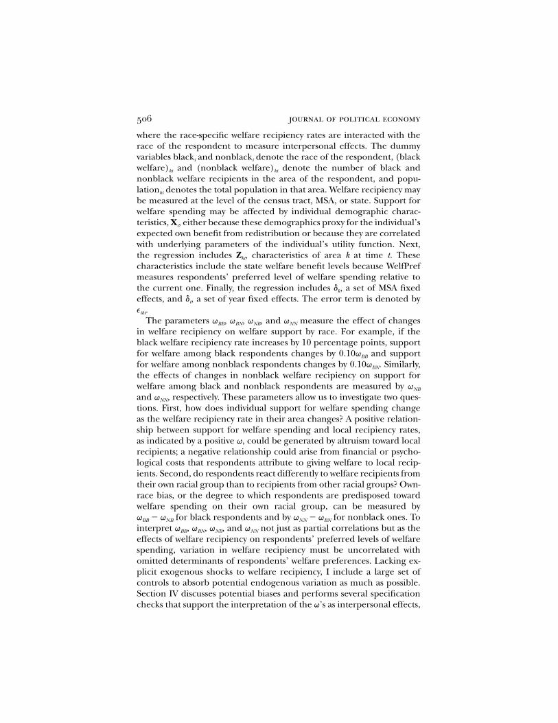
iency rate is .43 and the R2 for the racial composition of welfare recip-ients is .97. Second, I estimate welfare recipiency rates by race usingthe census Public Use Micro Sample (PUMS). Because the PUMS asksindividuals about receipt of public assistance, age, marital status, andthe presence of own children, AFDC recipiency can be estimated fairlyaccurately. The results in this paper concerning reactions to welfarerecipiency at the MSA or state level do not change substantially whenmeasures of welfare recipiency based on the PUMS are used instead ofthe STF measures. Details of both checks can be found in Luttmer(1999). Since the PUMS provides no information at the census tractlevel, I use the STF proxies for welfare recipiency in this paper. Becauseinformation only for 1970, 1980, and 1990 is available in the census,the values for the proxies between the census years are computed bylinear interpolation. The proxies for years after 1990 are equal to thevalues in 1990. The main results are robust to removing those yearsfrom the sample that rely most heavily on the interpolation (see Luttmer[1999] for details).

III. Empirical Strategy

A. Estimation of Interpersonal Effects

The basic empirical specification for the preferred level of welfarespending, WelfPrefikt, of individual i living in area k at time t is givenby2

(black welfare)ktWelfPref p black qikt i BBpopulationkt

(black welfare)kt� nonblack qi BNpopulationkt

(nonblack welfare)kt� black qi NBpopulationkt

(nonblack welfare)kt� nonblack qi NNpopulationkt

� X a � Z b � d � d � e ,i kt k t ikt

2 Although areas are indexed by a single subscript k, the reader should be aware thatarea characteristics in the same regression may be measured at different geographicallevels. Some area characteristics (e.g., welfare benefit levels) are by definition measuredonly at the state level. Area fixed effects are always measured at the MSA level becausethis is the most detailed level possible. Welfare recipiency is measured at the tract, MSA,or state level, as indicated in the tables.


where the race-specific welfare recipiency rates are interacted with therace of the respondent to measure interpersonal effects. The dummyvariables blacki and nonblacki denote the race of the respondent, (blackwelfare)kt and (nonblack welfare)kt denote the number of black andnonblack welfare recipients in the area of the respondent, and popu-lationkt denotes the total population in that area. Welfare recipiency maybe measured at the level of the census tract, MSA, or state. Support forwelfare spending may be affected by individual demographic charac-teristics, Xi, either because these demographics proxy for the individual’sexpected own benefit from redistribution or because they are correlatedwith underlying parameters of the individual’s utility function. Next,the regression includes Zkt, characteristics of area k at time t. Thesecharacteristics include the state welfare benefit levels because WelfPrefmeasures respondents’ preferred level of welfare spending relative tothe current one. Finally, the regression includes dk, a set of MSA fixedeffects, and dt, a set of year fixed effects. The error term is denoted byeikt.

The parameters qBB, qBN, qNB, and qNN measure the effect of changesin welfare recipiency on welfare support by race. For example, if theblack welfare recipiency rate increases by 10 percentage points, supportfor welfare among black respondents changes by 0.10qBB and supportfor welfare among nonblack respondents changes by 0.10qBN. Similarly,the effects of changes in nonblack welfare recipiency on support forwelfare among black and nonblack respondents are measured by qNB

and qNN, respectively. These parameters allow us to investigate two ques-tions. First, how does individual support for welfare spending changeas the welfare recipiency rate in their area changes? A positive relation-ship between support for welfare spending and local recipiency rates,as indicated by a positive q, could be generated by altruism toward localrecipients; a negative relationship could arise from financial or psycho-logical costs that respondents attribute to giving welfare to local recip-ients. Second, do respondents react differently to welfare recipients fromtheir own racial group than to recipients from other racial groups? Own-race bias, or the degree to which respondents are predisposed towardwelfare spending on their own racial group, can be measured by

for black respondents and by for nonblack ones. Toq � q q � qBB NB NN BN

interpret qBB, qBN, qNB, and qNN not just as partial correlations but as theeffects of welfare recipiency on respondents’ preferred levels of welfarespending, variation in welfare recipiency must be uncorrelated withomitted determinants of respondents’ welfare preferences. Lacking ex-plicit exogenous shocks to welfare recipiency, I include a large set ofcontrols to absorb potential endogenous variation as much as possible.Section IV discusses potential biases and performs several specificationchecks that support the interpretation of the q’s as interpersonal effects,

group loyalty 507

but as in any nonexperimental study, caution with this causal interpre-tation remains in order.

B. Predicted Tract-Level Welfare Recipiency

Estimates of own-race bias could be spurious if welfare recipiency ismeasured at the MSA level and the MSA is racially segregated. In thiscase, a nonblack individual may react more strongly to additional non-black welfare recipients than to additional black recipients because seg-regation makes it more likely for the individual to come into contactwith nonblack recipients than with black recipients. Estimates based onwelfare recipiency in census tracts would be much less susceptible tothis bias because the relatively small size of tracts implies that individualswould also come into contact with welfare recipients of other races.Though the GSS does not provide more detailed information about thelocation of respondents than their MSA, it is possible to use two-sampletwo-stage least squares (2SLS) to estimate how individuals respond towelfare recipiency in their neighborhood. Instead of using actual welfarerecipiency in the respondent’s tract, I use the expected tract-level welfarerecipiency conditional on the respondent’s characteristics and the pat-tern of race and income segregation in the MSA. Even if the tract ofGSS respondents had been known, using expected rather than actualwelfare recipiency would be preferable because it avoids Tiebout bias.The way in which individuals sort themselves into tracts with differentwelfare recipiency rates may be related to their preferences for welfarespending, which would bias the estimates.

The calculation of these expected welfare recipiency rates is describedin detail in Appendix B, but the intuition is simple. The census containsthe number of individuals who share a respondent’s MSA, incomebracket, and race. The fraction of these individuals who live in a givencensus tract equals the probability that the respondent lives in that tract.I calculate this probability for each tract and multiply tract-level welfarerecipiency rates by these probabilities to obtain the expected welfarerecipiency rates in that respondent’s census tract. Summary statistics onwelfare recipiency rates at the tract, MSA, and state levels can be foundin Appendix table A2.

The expected welfare recipiency rates can be interpreted as the resultof a first-stage regression, where the main instrument is the interactionof the race and income of the respondent with contemporaneous raceand income segregation in the MSA of the respondent. Only the in-teraction term is an instrument because the direct effects of the re-spondent’s income and race are absorbed by the demographic controlsand because the direct effects of segregation are largely absorbed by


the MSA fixed effects. The direct effects of segregation are fully absorbedonly if the MSA fixed effects are allowed to vary over time.

IV. Results

A. Effects of Demographics and Tract-Level Welfare Recipiency on Supportfor Welfare

Table 2 reports the baseline regression explaining individual supportfor welfare spending. Unless otherwise noted, the independent variablesin all regressions consist of measures of welfare recipiency, character-istics of the respondent’s area, demographic characteristics of the re-spondent, year fixed effects, and MSA fixed effects. In order to maximizethe sample size, the nonmetropolitan part of each state is treated asthough it were a single MSA, but the results are robust to omitting theseareas (Luttmer 1999). All three columns in table 2 come from a singleordinary least squares regression. The first column shows coefficientson variables that are not interacted with a race dummy, and the secondand third columns show coefficients on variables that are interactedwith a black and nonblack dummy. The regression includes two mea-sures of tract-level welfare recipiency: the expected ratio of black welfarerecipients to the tract population and a similar ratio for nonblack welfarerecipients. The other geographical characteristics include the expectedracial composition in the respondent’s tract, measured as the numberof black persons as a fraction of the tract population; the log of thepopulation in the town or city of the respondent; the maximum realAFDC benefits for a family of four in the respondent’s state in real 1990dollars; and the twenty-fifth percentile of the earnings distribution inthe respondent’s state. The demographic characteristics consist of therespondent’s race, gender, income, education, age, marital status, andhousehold composition. Because the regression includes MSA and yearfixed effects, it is driven by differential variation over time across MSAs.The regression has 18,764 observations in 138 MSAs, and these obser-vations occur in 1,447 MSA#year cells.

The most interesting result is how welfare support is affected by thenumber and race of welfare recipients in the respondent’s area. Theseestimates are indicated in boldface in table 2 and establish two maincharacteristics of interpersonal effects. First, they show a clear patternof racial group loyalty. In other words, an additional black welfare re-cipient in one’s tract reduces support for welfare by nonblack respon-dents but has little effect on black respondents. Conversely, an additionalnonblack welfare recipient reduces black support for welfare but haslittle effect on nonblack support. Second, they show a negative exposureeffect. A simultaneous increase of black and nonblack welfare recipiency

TABLE 2Baseline Regression (Np18,764)

Dependent Variable: Self-Reported Support for Welfare Spending

IndependentVariable

(NotInteracted)

IndependentVariable#Black

RespondentDummy

IndependentVariable

#NonblackRespondent

Dummy

Expected welfare recipiency in tract:Black recipients/population �.8 (.3) �6.7 (1.7)Nonblack recipients/population �3.7 (1.4) 2.0 (1.0)

Black .13 (.06)Other race .03 (.02)Female .006 (.005)Five-point spline in income/poverty line

(marginal effects):Bottom quintile �.13 (.03) �.18 (.02)Quintile 2 �.04 (.03) �.06 (.01)Quintile 3 �.02 (.04) �.02 (.01)Quintile 4 �.08 (.03) �.02 (.01)Top quintile �.004 (.007) .000 (.002)

High school diploma �.042 (.007)Some college �.056 (.015)College degree �.013 (.010)Graduate or professional degree .066 (.014)Age �.003 (.001)Age2/100 .002 (.001)Widowed .023 (.013)Divorced .017 (.013)Separated .035 (.019)Never married .032 (.011)Has had child/children �.023 (.009)Child present at home �.028 (.011)Single mother .016 (.016)2-person household .027 (.012)3-person household .046 (.014)4-person household .050 (.015)5 or more–person household .062 (.016)

Expected fraction black in tract .27 (.08) .80 (.23)Log population in town/city .008 (.002)Missing town/city population �.026 (.020)Maximum real AFDC benefit in state

($100s) �.010 (.005)25th percentile of earnings in state

($100/wk.) .028 (.027)Year fixed effects (18) yesMSA fixed effects (138) yesAdjusted R2 .156

Note.—The dependent variable is support for welfare spending as measured by the GSS. This variable is 1 forrespondents who think welfare spending is too low, 1/2 for those who think it is about right, and 0 for those who thinkit is too high. All coefficients in this table come from a single ordinary least squares regression. Standard errors (inparentheses) are corrected for group error terms in MSA#year cells. All variables that are interacted with race havebeen demeaned by their overall mean. Welfare recipiency measures are based on census STF information and describedin App. table A2.


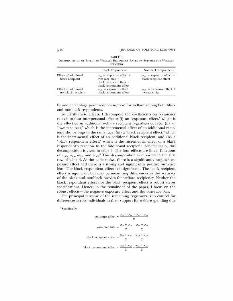
TABLE 3Decomposition of Effect of Welfare Recipiency Rates on Support for Welfare

Spending

Black Respondent Nonblack Respondent

Effect of additionalblack recipient

qBB p exposure effect �own-race bias �black recipient effect �black respondent effect

qBN p exposure effect �black recipient effect

Effect of additionalnonblack recipient

qNB p exposure effect �black respondent effect

qNN p exposure effect �own-race bias

by one percentage point reduces support for welfare among both blackand nonblack respondents.

To clarify these effects, I decompose the coefficients on recipiencyrates into four interpersonal effects: (i) an “exposure effect,” which isthe effect of an additional welfare recipient regardless of race; (ii) an“own-race bias,” which is the incremental effect of an additional recip-ient who belongs to the same race; (iii) a “black recipient effect,” whichis the incremental effect of an additional black recipient; and (iv) a“black respondent effect,” which is the incremental effect of a blackrespondent’s reaction to the additional recipient. Schematically, thisdecomposition is given in table 3. The four effects are linear functionsof qBB, qBN, qNB, and qNN.3 This decomposition is reported in the firstrow of table 4. As the table shows, there is a significantly negative ex-posure effect and there is a strong and significantly positive own-racebias. The black respondent effect is insignificant. The black recipienteffect is significant but may be measuring differences in the accuracyof the black and nonblack proxies for welfare recipiency. Neither theblack respondent effect nor the black recipient effect is robust acrossspecifications. Hence, in the remainder of the paper, I focus on therobust effects—the negative exposure effect and the own-race bias.

The principal purpose of the remaining regressors is to control fordifferences across individuals in their support for welfare spending due

3 Specifically,

q � q � q � qBN NB NN BBexposure effect p ,2

q � q q � qBB NN BN NBown-race bias p � ,2 2

q � q q � qBB BN NB NNblack recipient effect p � ,2 2

q � q q � qBB NB BN NNblack respondent effect p � .2 2

group loyalty 511

to financial self-interest or underlying tastes. In fact, without these in-dividual controls, the negative exposure effect would disappear. Therespondent’s race is among the strongest predictors for welfare support.At the sample mean, blacks are 13 percent more likely to respond thatwelfare spending is too low than whites with the same characteristicsliving in the same area.4 The response from people who are neitherblack nor white is not significantly different from the white response,which is reassuring since they are grouped with whites in race-basedinteraction terms. Gender seems to have little effect on welfare support.For both blacks and nonblacks, income has a negative and convex effecton support for welfare. The effects of additional income are strongestat the lowest income quintile, where nonblacks are 18 percent morelikely to respond that welfare spending is too high (compared to think-ing it is too low) if their income rises by the amount of the poverty line($15,029 for a couple with two children in 1994). At higher incomelevels, the marginal effect of income on welfare support generally re-mains negative but becomes less strong. Education shows a U-shapedpattern in which those with graduate or professional degrees displaymore support for welfare spending than high school dropouts. Theincome results support the notion that support for welfare spendingcan be partially explained by direct self-interest. People with higherincomes are less likely to receive welfare benefits themselves, and theywould therefore be less likely to support welfare spending if they con-sider only the financial costs and benefits of redistribution to themselves.The marginal effect of income on the likelihood of welfare receipt isespecially strong at the lowest income levels, which is consistent withthe regression results. Education also lowers the likelihood of welfarereceipt, which explains the decrease in support for welfare spendingfor initial increases in education. The higher levels of welfare supportamong the most highly educated respondents cannot be easily explainedby self-interest. Other results consistent with self-interest are the declineof support for welfare with age (until the age of 75) and higher supportamong single women relative to married women. Contrary to the pre-dictions of self-interest, welfare support is lowered by the presence ofchildren and by ever having had children.

The expected fraction of black persons in area k is included as acontrol to ensure that the findings on welfare recipiency are driven bythe race of welfare recipients, and not merely by the racial compositionof the area. The positive effect of city or town population on welfaresupport may indicate that residents of larger cities are more likely toreceive welfare after observables are controlled for. Higher state AFDC

4 The race dummy can be interpreted like this because all variables that are interactedwith race are expressed in deviations from the sample mean.

512

TABLE 4Effect of Welfare Recipiency at Different Geographical Levels (Np18,764)


Effects of Welfare RecipiencyAll EffectsJointly Zero(p-Value) 2RExposure Effect Own-Race Bias Black Recipient Effect

Black RespondentEffect

1. Expected tract recipiency �3.8(1.2)

5.8(1.3)

�2.9(1.3)

�.1(.9)

.0000 .1561

2. MSA recipiency �8.0(2.5)

5.6(1.5)

3.8(2.3)

�4.0(.9)

.0000 .1556

3. State recipiency �4.2(3.1)

5.8(2.1)

�.2(3.1)

�4.8(1.1)

.0000 .1550

4. Tract and MSA recipiency:Expected tract recipiency �2.9

(1.5)4.6

(1.9)�3.8(1.8)

1.6(1.5)

.03 .1565

MSA recipiency �5.7(3.0)

2.6(2.3)

4.3(2.9)

�3.0(1.8)

.26

t-statistic on coefficientdifference

[.7] [.5] [�2.0] [1.5] .16

t-statistic on coefficient sum [�3.3] [4.0] [.2] [�1.1]

5. Tract and state recipiency:Expected tract recipiency �3.7

(1.3)5.0

(1.6)�2.5(1.6)

1.1(1.3)

.02 .1562

State recipiency �.7(3.3)

.9(2.5)

�.9(3.2)

�3.1(1.9)

.30


[�.8] [1.2] [�.4] [1.4] .32

t-statistic on coefficient sum [�1.4] [2.7] [�1.2] [�1.4]

513

6. MSA and state recipiency:MSA recipiency �10.4

(3.0)6.7

(2.1)8.0

(2.9)�2.2(2.0)

.008 .1558

State recipiency 4.0(3.7)

�1.2(2.8)

�6.6(3.7)

�2.6(2.5)

.09


[�2.5] [1.8] [2.5] [.1] .11

t-statistic on coefficient sum [�2.0] [2.6] [.5] [�4.1]

Note.—The dependent variable is support for welfare spending as measured by the GSS. This variable is 1 for respondents who think welfare spending is too low, 1/2 for those whothink it is about right, and 0 for those who think it is too high. Only the decomposition of the coefficients on welfare recipiency rates is reported. All regressions contain the samecontrols as in table 2. They include individual demographics as well as 138 MSA and 18 year fixed effects. Standard errors (in parentheses) are corrected for group error terms inMSA#year cells. Welfare recipiency measures are based on census STF information and described in App. table A2.


benefits reduce welfare support, which one would expect since the ques-tion asks respondents about welfare spending relative to the currentlevel. The coefficient on the twenty-fifth percentile of the earnings dis-tribution in the state, which Moffitt, Ribar, and Wilhelm (1998) use asa proxy for potential labor market earnings for welfare recipients, isinsignificant.

B. The Effect of Geographical Proximity to Welfare Recipients

The previous subsection presented evidence of interpersonal effects atthe census tract level. This subsection explores how respondents’ welfaresupport is affected by the race and prevalence of welfare recipients atdifferent geographical levels. The first line of table 4 replicates theregression with expected tract-level recipiency measures that was re-ported in full in table 2. The second and third rows show the sameregression, but with MSA- and state-level recipiency measures, respec-tively. At the MSA level, the exposure effect is significantly negative andmore than twice as large as at the tract level. At the state level, theexposure effect is large and negative as well, but not significant. At boththe MSA and state levels, the estimate for the own-race bias is significantand about as large as at the tract level. These regressions indicate thatinterpersonal preferences operate at each of the three geographicallevels considered. Interpersonal preferences consistently show an own-race bias and a negative exposure effect, but they seem to depend onthe geographical level for the black recipient and black respondenteffect.

In regressions 4, 5, and 6, recipiency measures of two geographiclevels are included in each regression to sort out better at which levelinterpersonal preferences operate most strongly. In the regression withboth tract- and MSA-level measures, the negative exposure effect andthe own-race bias operate at both levels, but the standard errors arerelatively large because of multicollinearity. The comparison of tract- tostate-level measures shows that the exposure effect and own-race biasoperate more strongly at the tract level than at the state level, but thesedifferences are not statistically significant. The final regression showsthat these two interpersonal effects also operate more strongly at theMSA level than at the state level. It seems, therefore, that the exposureeffect and own-race bias are determined mostly at the tract level andthe MSA level but are hardly affected by state-level recipiency after tract-and MSA-level measures are included.

The table provides two insights. First, the negative exposure effectand racial group loyalty seem to be affected most by local welfare re-cipiency rates. Second, these two interpersonal effects are still significantat the tract and MSA levels after state-level recipiency rates are controlled

group loyalty 515

for. Given that welfare policy is determined at the state level, state-levelrecipiency rates determine the effective cost to taxpayers of a dollar ofredistribution. Hence, the effect of state-level recipiency rates on sup-port for welfare spending could partially reflect financial self-interest.However, when controls for state-level recipiency are included, any effectof local recipiency rates on support for welfare indicates the presenceof interpersonal effects.5

C. Specification Checks

This subsection investigates the possibility that omitted variable biasesdrive the results. One might believe that a higher local welfare recipiencyrate signals that the respondent has unobservable traits that increasethe respondent’s welfare support due to self-interest. In this case, onewould expect to find a spurious positive relationship between local re-cipiency rates and welfare support. However, the negative exposure ef-fect shows that higher local recipiency rates decrease welfare support.Table 5 provides three additional types of evidence against the omittedvariable bias explanation.

First, if a variable were omitted that is correlated with both the re-spondent’s likelihood of receiving welfare and local welfare recipiency,one would expect such an omitted variable to be much more importantfor respondents who are potential welfare recipients than for respon-dents who are unlikely welfare recipients. To test this, I allow a differenteffect of tract-level welfare recipiency on respondents with incomes be-low 200 percent of the poverty line and those with incomes above 200percent of the poverty line. Because respondents with incomes above200 percent of the poverty line are much less likely to be or becomewelfare recipients, one would expect the effect of recipiency to be muchsmaller if the results were driven by omitted variable bias.6 As regression1 shows, the exposure effect and the own-race bias are at least as strongfor respondents with incomes above 200 percent of the poverty line asfor poorer respondents.

Second, one might worry that the difference between black and non-black unobservables varies across cities. In regression 2, I include MSAfixed effects separately by race. The significance and the magnitude ofthe exposure effect and own-race bias remain largely the same.

5 If individuals’ perceptions of the state-level welfare recipiency rate are influenced bythe local recipiency rate, their support for welfare spending could depend on the localrecipiency rate even in the absence of interpersonal effects. Luttmer (1999) tests thishypothesis and finds no support for it.

6 Of course, people with incomes above 200 percent of the poverty line could have closerelatives on welfare. As long as we would expect them to be less likely to have such relativesthan individuals with incomes below 200 percent of the poverty line, this check for omittedvariable bias remains valid.

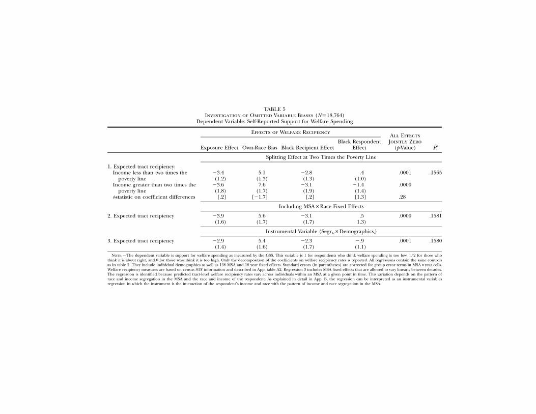
TABLE 5Investigation of Omitted Variable Biases (Np18,764)


Effects of Welfare RecipiencyAll Effects

Jointly Zero(p-Value) 2RExposure Effect Own-Race Bias Black Recipient Effect

Black RespondentEffect

Splitting Effect at Two Times the Poverty Line

1. Expected tract recipiency:Income less than two times the

poverty line�3.4(1.2)

5.1(1.3)

�2.8(1.3)

.4(1.0)

.0001 .1565

Income greater than two times thepoverty line

�3.6(1.8)

7.6(1.7)

�3.1(1.9)

�1.4(1.4)

.0000

t-statistic on coefficient differences [.2] [�1.7] [.2] [1.3] .28

Including MSA#Race Fixed Effects


5.6(1.7)

�3.1(1.7)

.51.3)

.0000 .1581

Instrumental Variable (Segrkt#Demographicsi)


5.4(1.6)

�2.3(1.7)

�.9(1.1)

.0001 .1580

Note.—The dependent variable is support for welfare spending as measured by the GSS. This variable is 1 for respondents who think welfare spending is too low, 1/2 for those whothink it is about right, and 0 for those who think it is too high. Only the decomposition of the coefficients on welfare recipiency rates is reported. All regressions contain the same controlsas in table 2. They include individual demographics as well as 138 MSA and 18 year fixed effects. Standard errors (in parentheses) are corrected for group error terms in MSA#year cells.Welfare recipiency measures are based on census STF information and described in App. table A2. Regression 3 includes MSA fixed effects that are allowed to vary linearly between decades.The regression is identified because predicted tract-level welfare recipiency rates vary across individuals within an MSA at a given point in time. This variation depends on the pattern ofrace and income segregation in the MSA and the race and income of the respondent. As explained in detail in App. B, the regression can be interpreted as an instrumental variablesregression in which the instrument is the interaction of the respondent’s income and race with the pattern of income and race segregation in the MSA.

group loyalty 517

Third, MSA fixed effects might not be adequate if the unobservablesof the population in an MSA change over time in a way that is correlatedwith welfare recipiency. Because the welfare recipiency measures arebased on linear interpolations between decades, a set of MSA-specificlinear splines with knots at the decades can fully absorb any correlationbetween MSA-specific time variation in unobservables and welfare re-cipiency measures. In regression 3, such a set of MSA-specific splines isincluded, and the results are essentially the same as before. This re-gression is fully driven by the interaction of the race and income ofrespondents with the pattern of race and income segregation in theMSA. It can therefore be interpreted as an instrumental variables re-gression, where the instrument is this interaction term (see App. B fordetails).

V. Self-Reported Preferences and Voting Behavior

If self-reported preferences on welfare spending accurately reflect un-derlying preferences, then these self-reported preferences should cor-respond closely to voting behavior. I examine the validity of the self-reported preference measure by testing whether it predicts votingoutcomes on California’s Proposition 165 from the 1992 primaries. Thisproposition, drafted by former governor Pete Wilson, proposed bothcuts in welfare generosity and changes in the state budget process. Thesummary of the proposition in the September 1992 issue of the CaliforniaJournal reads as follows: “An initiative constitutional amendment thatgrants the governor the power to declare a ‘fiscal emergency’ when thebudget is not adopted or the deficit exceeds specified percentages. Italso reduces aid to families with dependent children (AFDC) by 10percent, then by an additional 15 percent after six months on aid.”7

Public information on Proposition 165 emphasized its importance forwelfare. For example, when describing the outcomes of propositions,the California Journal listed that “Proposition 165 (welfare)” was rejectedby 54 percent of the voters.

Election outcomes of Proposition 165 are available for the 30,000election precincts in California. The Institute for Governmental Studiesat the University of California at Berkeley merged precinct-level votingreturns to census blocks and then aggregated the data into about 20,000

7 In addition, the proposition specified that AFDC benefits could not increase becauseof the birth of a child that was conceived while the family was receiving aid and that,during the first 12 months of residency in California, recipients could not receive higherbenefits than what they would have received in their former state. It also specified anelimination of all special benefits to pregnant women and a $50 reward for AFDC parentsunder age 19 attending high school if they had no more than two unexcused absencesand no more than four total absences per month. Those who had more absences wouldface a $50 penalty.


TABLE 6Regressions of California Vote on Proposition 165 (Welfare Cuts) (Np20,668

Block Groups)Dependent Variable: Percentage Votes against Proposition 165 (Cuts in Welfare

Spending)

Independent Variable (1) (2) (3) (4)

Predicted support forwelfare (GSS)

1.112(.009)

1.082(.008)

.709(.011)

.783(.013)

Percentage black inblock group

.201(.005)

Constant term .108(.004)

NA NA .232(.005)

County fixed effects? no yes no noTract fixed effects? no no yes noAdjusted R2 .407 .657 .755 .448

Note.—Standard errors are in parentheses. Predicted support for welfare is constructed as follows: First self-reportedsupport for welfare spending from the GSS is regressed on a set of 20 individual demographic characteristics as wellas MSA and year fixed effects. This regression is the same as the baseline regression in table 2, except that the regressorsare limited to demographic characteristics from the GSS that are also available in the 1990 Census STF. Next, I predictwelfare support in each block group by multiplying the block group demographics (from the census) with the corre-sponding coefficients from the regression of GSS welfare support on individual demographics.

block groups. I match voting data to demographic information fromthe 1990 Census STF, coding demographic variables to correspondclosely to the ones available in the GSS.8

To assess whether self-reported preferences for welfare spending cor-respond to voting behavior, I first use the GSS data to regress self-reported support for welfare spending (WelfPref) on a set of 20 indi-vidual demographic characteristics as well as MSA and year fixed effects.This regression is the same as the baseline regression in table 2, exceptthat the regressors are limited to demographic characteristics from theGSS that are also available in the 1990 Census STF (see Luttmer [1999]for details). Next, I predict welfare support in each block group bymultiplying the block group demographics (from the census) with thecorresponding coefficients in the regression of GSS welfare support onindividual demographics. This predictor is constructed without usingany information from the voting outcomes. Column 1 of table 6 showsthat actual voting outcomes can be explained extraordinarily well bypredicted welfare support.9 Columns 2, 3, and 4 show that the results

8 The demographic information consists of three race dummies, gender, single moth-erhood, five marital status dummies, five educational attainment dummies, five householdsize dummies, age, age squared, a linear trend for income below 200 percent of the povertyline, and a dummy for income above 200 percent of the poverty line. The income spec-ification was chosen because the STF contains a relatively fine breakdown of income asa percentage of the poverty line until 200 percent of the poverty line but no breakdownof incomes above 200 percent of the poverty line. When omitted categories are excluded,this yields a set of 20 demographic regressors.

9 The predicted support for welfare is systematically lower than the fraction of votesagainst welfare cuts. This could be due to differences in framing of the GSS question andthe ballot question or to selective voter turnout.

group loyalty 519

remain strong and highly significant when county fixed effects, tractfixed effects, or the fraction black in the block group is added as acontrol. These results suggest that self-reported preferences are a usefulmeasure of underlying preferences.

VI. Discussion

The previous sections documented that self-reported welfare attitudescan be used to estimate the impact of interpersonal effects on supportfor redistribution. In particular, I have shown that interpersonal pref-erences exhibit both a negative exposure effect and racial group loyalty.These findings validate theoretical models that include interpersonaleffects. More important, empirical evidence on interpersonal prefer-ences is useful because it improves our understanding of the forcesdriving redistribution.

The generosity of redistribution varies widely across states and coun-tries, and many have noted that relatively homogeneous areas tend tohave more income redistribution and other forms of public spending(Orr 1976; Easterly and Levine 1997; Poterba 1997; Alesina et al. 1999).Consistent with this observation, the United States is relatively racially,ethnically, and religiously heterogeneous and redistributes less thanmost western European countries. Within the United States, relativelyracially heterogeneous states provide lower welfare benefits (fig. 2).

While the correlation between demographic homogeneity and gen-erosity of redistribution has been well established, there is little evidenceon the mechanisms underlying this correlation. Easterly and Levine(1997) and Alesina et al. (1999) posit that demographic fragmentationaffects redistribution because it influences how the political processaggregates individual preferences. Interpersonal preferences provide acomplementary explanation. If individuals prefer to redistribute to theirown racial, ethnic, or religious group, they prefer less redistributionwhen members of their own group constitute a smaller share of ben-eficiaries. As demographic heterogeneity increases, on average, theshare of beneficiaries belonging to one’s own group declines. Thusaverage support for redistribution declines as heterogeneity increases.

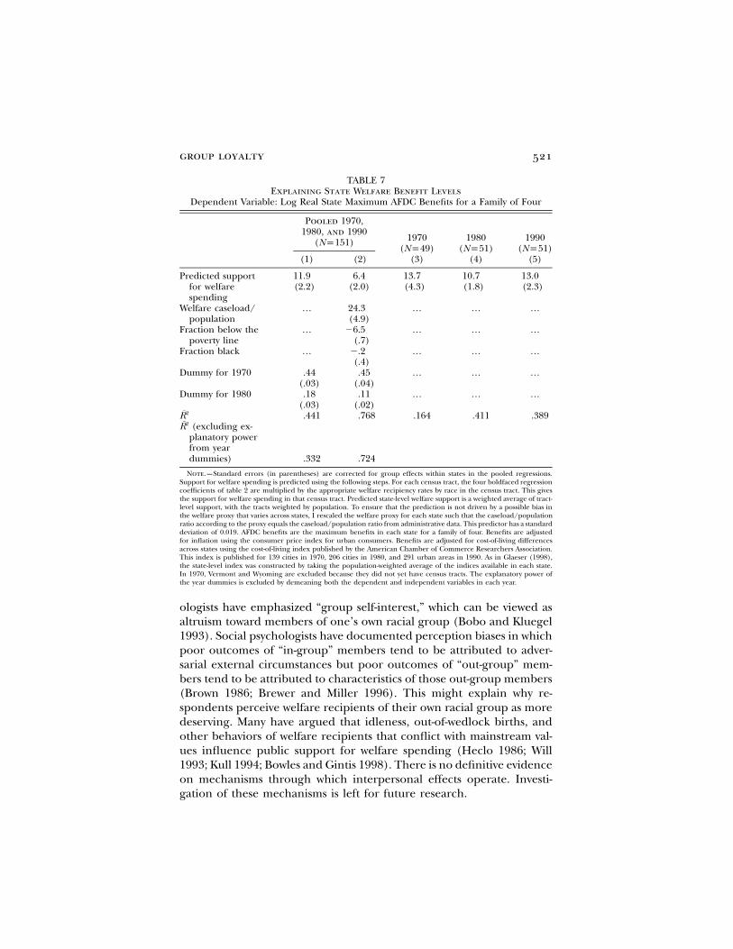
To measure whether interpersonal effects partially explain the rela-tionship between demographic heterogeneity and redistribution, I re-late differences in state-level welfare benefits to a predictor of welfaresupport based solely on interpersonal preferences and the demographiccomposition in each state. The construction of this predictor is ex-plained in detail in Appendix B. Column 1 of table 7 shows that thispredictor can explain 33 percent of the variation across states in thelog real AFDC benefits for 1970, 1980, and 1990. This figure is quitelarge given that coefficient estimates used to predict welfare are based


Fig. 2.—Correlation between real AFDC benefits and racial heterogeneity, 1990. Racialheterogeneity is defined as the probability that two randomly selected persons belong toa different racial group, where the racial groups are black and nonblack: racial hetero-geneity p 1 � (fraction black)2 � (fraction nonblack)2. AFDC benefits are the maximumbenefits in each state for a family of four. Benefits are adjusted for cost-of-living differencesacross states using the cost-of-living index published by the American Chamber of Com-merce Researchers Association. This index is published for 291 urban areas in 1990. Asin Glaeser (1998), the state-level index was constructed by taking the population-weightedaverage of the indices for the urban areas. The regression line has a slope of �2.32 witha standard error of .38. Adjusted ; there are 51 observations. The correlation2R p .42remains negative and significant if Mississippi and Alabama are dropped.

on variation within states. Column 2 shows that the predictor remainssignificant when the state-level welfare caseload, the state poverty rate,and the fraction black in the state are added as controls. Thus the welfarepredictor captures how individuals respond to welfare recipients of an-other race, and not the fraction black, the poverty rate, or the averagelevel of welfare recipiency in their area. Columns 3–5 show that thepredictor is also significant for each year separately.

While data constraints restrict my analysis to racial heterogeneity inthe United States, heterogeneity in other dimensions, such as ethnicityor religion, is likely to be important as well. Similarly, it seems plausiblethat the effects of racial, ethnic, or religious group loyalty apply to otherredistributive policies and to other countries. This suggests that inter-personal effects can explain why the heterogeneity of the U.S. popu-lation compared to western European countries leads to relatively lowlevels of redistribution in the United States.

This paper argues that interpersonal preferences help explain therelation between ethnic fragmentation and redistribution, but are theredeeper mechanisms that can explain interpersonal preferences? Soci-

group loyalty 521

TABLE 7Explaining State Welfare Benefit Levels

Dependent Variable: Log Real State Maximum AFDC Benefits for a Family of Four

Pooled 1970,1980, and 1990

(Np151) 1970(Np49)

(3)

1980(Np51)

(4)

1990(Np51)

(5)(1) (2)

Predicted supportfor welfarespending

11.9(2.2)

6.4(2.0)

13.7(4.3)

10.7(1.8)

13.0(2.3)

Welfare caseload/population

… 24.3(4.9)

… … …

Fraction below thepoverty line

… �6.5(.7)

… … …

Fraction black … �.2(.4)

… … …

Dummy for 1970 .44(.03)

.45(.04)

… … …

Dummy for 1980 .18(.03)

.11(.02)

… … …

2R .441 .768 .164 .411 .389(excluding ex-2R

planatory powerfrom yeardummies) .332 .724

Note.—Standard errors (in parentheses) are corrected for group effects within states in the pooled regressions.Support for welfare spending is predicted using the following steps. For each census tract, the four boldfaced regressioncoefficients of table 2 are multiplied by the appropriate welfare recipiency rates by race in the census tract. This givesthe support for welfare spending in that census tract. Predicted state-level welfare support is a weighted average of tract-level support, with the tracts weighted by population. To ensure that the prediction is not driven by a possible bias inthe welfare proxy that varies across states, I rescaled the welfare proxy for each state such that the caseload/populationratio according to the proxy equals the caseload/population ratio from administrative data. This predictor has a standarddeviation of 0.019. AFDC benefits are the maximum benefits in each state for a family of four. Benefits are adjustedfor inflation using the consumer price index for urban consumers. Benefits are adjusted for cost-of-living differencesacross states using the cost-of-living index published by the American Chamber of Commerce Researchers Association.This index is published for 139 cities in 1970, 206 cities in 1980, and 291 urban areas in 1990. As in Glaeser (1998),the state-level index was constructed by taking the population-weighted average of the indices available in each state.In 1970, Vermont and Wyoming are excluded because they did not yet have census tracts. The explanatory power ofthe year dummies is excluded by demeaning both the dependent and independent variables in each year.

ologists have emphasized “group self-interest,” which can be viewed asaltruism toward members of one’s own racial group (Bobo and Kluegel1993). Social psychologists have documented perception biases in whichpoor outcomes of “in-group” members tend to be attributed to adver-sarial external circumstances but poor outcomes of “out-group” mem-bers tend to be attributed to characteristics of those out-group members(Brown 1986; Brewer and Miller 1996). This might explain why re-spondents perceive welfare recipients of their own racial group as moredeserving. Many have argued that idleness, out-of-wedlock births, andother behaviors of welfare recipients that conflict with mainstream val-ues influence public support for welfare spending (Heclo 1986; Will1993; Kull 1994; Bowles and Gintis 1998). There is no definitive evidenceon mechanisms through which interpersonal effects operate. Investi-gation of these mechanisms is left for future research.

522

Appendix A

TABLE A1Summary Statistics for the GSS Sample: Means (and Standard Deviations)

VariableAll Observations

(Np18,764)

Respondent Believes Welfare Spending Is:

Too High(Supportp0)(Np9,635)

About Right(Supportp )1

2(Np5,419)

Too Low(Supportp1)(Np3,710)

Support for welfare (WelfPref) .34 (.39) 0 (0) 1/2 (0) 1 (0)Black .13 (.33) .06 (.24) .12 (.33) .29 (.46)White .86 (.35) .92 (.27) .86 (.35) .69 (.46)Other .02 (.13) .02 (.12) .02 (.14) .02 (.14)Household income in:

Quintile 1 .20 (.40) .12 (.33) .22 (.41) .36 (.48)Quintile 2 .20 (.40) .20 (.40) .21 (.41) .21 (.40)Quintile 3 .20 (.40) .22 (.41) .20 (.40) .17 (.37)Quintile 4 .20 (.40) .23 (.42) .19 (.39) .15 (.35)Quintile 5 .20 (.40) .24 (.42) .18 (.38) .12 (.33)

Female .54 (.50) .53 (.50) .55 (.50) .58 (.49)Married .61 (.49) .67 (.47) .58 (.49) .51 (.50)Widowed .10 (.29) .09 (.28) .11 (.31) .10 (.30)Divorced .10 (.29) .09 (.29) .09 (.29) .11 (.31)Separated .04 (.18) .03 (.16) .03 (.18) .06 (.24)Never married .16 (.37) .13 (.34) .18 (.39) .22 (.41)High school dropout .28 (.45) .24 (.43) .28 (.45) .37 (.48)High school diploma .51 (.50) .55 (.50) .50 (.50) .45 (.50)Some college .04 (.19) .04 (.19) .03 (.18) .03 (.17)College degree .12 (.32) .12 (.33) .12 (.33) .09 (.29)Graduate or professional degree .05 (.22) .05 (.21) .06 (.24) .05 (.22)Age 44.2 (17.2) 44.7 (16.6) 44.9 (18.1) 42.1 (17.3)1-person household .19 (.39) .18 (.38) .21 (.40) .19 (.39)2-person household .32 (.46) .33 (.47) .32 (.47) .28 (.45)

523

3-person household .18 (.39) .18 (.39) .18 (.38) .18 (.38)4-person household .17 (.37) .17 (.38) .16 (.37) .16 (.37)5 or more–person household .15 (.36) .14 (.35) .14 (.35) .19 (.39)Has had child/children .73 (.44) .75 (.43) .71 (.45) .71 (.45)Child present at home .44 (.50) .44 (.50) .42 (.49) .48 (.50)Single mother .07 (.26) .05 (.22) .07 (.26) .13 (.33)AFDC benefit in state ($100s) 5.64 (2.26) 5.75 (2.28) 5.62 (2.21) 5.39 (2.24)25th percentile of earnings ($100/wk.) 2.30 (.25) 2.31 (.25) 2.29 (.25) 2.29 (.25)Log population in town/city 3.31 (2.23) 3.11 (2.16) 3.33 (2.22) 3.82 (2.36)Missing town/city population .02 (.15) .03 (.16) .02 (.15) .01 (.11)Not in an MSA .36 (.48) .38 (.48) .36 (.48) .32 (.47)New England .05 (.21) .05 (.21) .05 (.21) .04 (.20)Mid Atlantic .16 (.36) .16 (.37) .16 (.36) .14 (.35)East North Central .21 (.41) .21 (.41) .21 (.40) .20 (.40)West North Central .08 (.27) .07 (.26) .08 (.28) .07 (.26)South Atlantic .18 (.39) .19 (.39) .17 (.38) .19 (.40)East South Central .07 (.25) .06 (.23) .07 (.25) .08 (.28)West South Central .09 (.28) .08 (.28) .08 (.28) .09 (.29)Mountain .05 (.22) .05 (.22) .06 (.23) .05 (.21)Pacific .13 (.34) .13 (.33) .13 (.34) .13 (.34)

Note.—Income is household income as a percentage of the poverty line. Household income quintiles are determined relative to all observations in the GSS with nonmissing household incomedata. The break points between the quintiles occur at 131 percent, 228 percent, 332 percent, and 506 percent of the poverty line. AFDC benefits are the maximum AFDC benefits for a family of fourin 1990 dollars. The twenty-fifth percentile of the earnings is based on the distribution of real weekly earnings of privately employed workers (self-employed workers are excluded) measured in hundredsof 1990 dollars (source: May Current Population Survey for 1973–80 and the Current Population Survey Merged Outgoing Rotation Groups for 1980–94).


TABLE A2Summary Statistics for Measures of Welfare Recipiency

AllRespondents(Np18,764)

BlackRespondents

(Np2,346)

NonblackRespondents(Np16,418)

MeanStandardDeviation Mean

StandardDeviation Mean

StandardDeviation

Black welfare recipiencyin expected tract .0118 .0243 .0626 .0396 .0046 .0052

White welfare recipiencyin expected tract .0091 .0074 .0092 .0094 .0091 .0071

Black welfare recipiencyin MSA .0106 .0102 .0174 .0122 .0097 .0096

White welfare recipiencyin MSA .0092 .0062 .0083 .0055 .0093 .0063

Black welfare recipiencyin state .0097 .0082 .0142 .0113 .0091 .0074

White welfare recipiencyin state .0081 .0048 .0076 .0043 .0081 .0048

Measures of the Fraction Black

Fraction blackin expected tract .1239 .1867 .5780 .1609 .0591 .0498

Fraction blackin MSA .1154 .0860 .1800 .0811 .1062 .0823

Fraction blackin state .1198 .0752 .1663 .0907 .1131 .0703

Note.—The nonmetropolitan parts of each state are treated as though they formed a single MSA. On the basis ofcomparisons with administrative data, these proxies are fairly accurate for the caseload by race divided by the totalpopulation. This rate is about three times as low as the number of welfare recipients divided by the total populationbecause each welfare case has, on average, three recipients (one mother and two children). The welfare recipiencyand racial composition variables are based on information from the census STF. The proxy for black welfare recipiencyas a fraction of the tract population is calculated as (black female–headed families/total families)#(black persons belowpoverty/total black persons), where all counts are performed at the tract level. The proxy for nonblack welfare recipiencyis formed analogously. These proxies are validated in Luttmer (1999). Because the census STF is available only for1970, 1980, and 1990, the welfare recipiency and racial composition variables for the years in between are formed bylinear interpolation, and the 1990 variables are used for 1991–94. The MSA-level variables are formed by taking aweighted average of the variables for the tracts that constitute the MSA; the weights are given by the number of familiesin the tract divided by the total number of families in the MSA. The aggregation for the state level is done similarly.

Appendix B

Construction of Expected Welfare Recipiency Rates

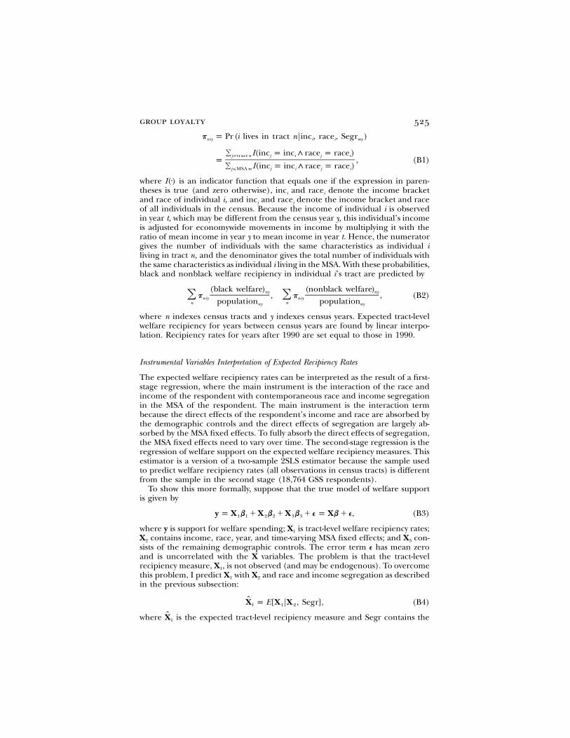
While the GSS does not provide more detailed information about the locationof respondents than their MSA, it is possible to use a procedure similar to 2SLSto estimate whether individuals respond to the rate and composition of welfarerecipiency in their neighborhood. Instead of using the actual welfare recipiencyin the census tract of an individual, I use predicted tract-level welfare recipiencybased on the individual’s characteristics and census information on the patternof race and income segregation in the MSA. Race and income segregation inan MSA m in census year y is denoted by Segrmy, which is not a one-dimensionalnumber but reflects the full distribution of race and income across the tractsin this MSA. Conditional on the race and income segregation in census year yin MSA m of individual i, the probability that this individual lives in tract n isgiven by

group loyalty 525

p p Pr (i lives in tract nFinc , race , Segr )niy i i my

� I(inc p inc ∧ race p race )j�tract n j i j ip , (B1)� I(inc p inc ∧ race p race )j�MSA m j i j i

where is an indicator function that equals one if the expression in paren-I(7)theses is true (and zero otherwise), inci and racei denote the income bracketand race of individual i, and incj and racej denote the income bracket and raceof all individuals in the census. Because the income of individual i is observedin year t, which may be different from the census year y, this individual’s incomeis adjusted for economywide movements in income by multiplying it with theratio of mean income in year y to mean income in year t. Hence, the numeratorgives the number of individuals with the same characteristics as individual iliving in tract n, and the denominator gives the total number of individuals withthe same characteristics as individual i living in the MSA. With these probabilities,black and nonblack welfare recipiency in individual i’s tract are predicted by

(black welfare) (nonblack welfare)ny nyp , p , (B2)� �niy niypopulation populationn nny ny

where n indexes census tracts and y indexes census years. Expected tract-levelwelfare recipiency for years between census years are found by linear interpo-lation. Recipiency rates for years after 1990 are set equal to those in 1990.

Instrumental Variables Interpretation of Expected Recipiency Rates

The expected welfare recipiency rates can be interpreted as the result of a first-stage regression, where the main instrument is the interaction of the race andincome of the respondent with contemporaneous race and income segregationin the MSA of the respondent. The main instrument is the interaction termbecause the direct effects of the respondent’s income and race are absorbed bythe demographic controls and the direct effects of segregation are largely ab-sorbed by the MSA fixed effects. To fully absorb the direct effects of segregation,the MSA fixed effects need to vary over time. The second-stage regression is theregression of welfare support on the expected welfare recipiency measures. Thisestimator is a version of a two-sample 2SLS estimator because the sample usedto predict welfare recipiency rates (all observations in census tracts) is differentfrom the sample in the second stage (18,764 GSS respondents).

To show this more formally, suppose that the true model of welfare supportis given by

y p X b � X b � X b � e p Xb � e, (B3)1 1 2 2 3 3

where y is support for welfare spending; X1 is tract-level welfare recipiency rates;X2 contains income, race, year, and time-varying MSA fixed effects; and X3 con-sists of the remaining demographic controls. The error term e has mean zeroand is uncorrelated with the X variables. The problem is that the tract-levelrecipiency measure, X1, is not observed (and may be endogenous). To overcomethis problem, I predict X1 with X2 and race and income segregation as describedin the previous subsection:

X p E[X FX , Segr], (B4)1 1 2

where is the expected tract-level recipiency measure and Segr contains theX1


income and racial composition of all census tracts in each MSA. Any conditionalexpectation, like equation (B4), can be rewritten as

ˆX p X � h, (B5)1 1

where the error term, h, has mean zero and is uncorrelated with the predictor.Hence, Moreover, the error term is not correlated in expectation′Ê[X h] p 0.1

with those variables used in predicting the expected recipiency rate. This impliesthat However, the information in X3 was not used to calculate the′Ê[X h] p 0.2

expected recipiency rates.10 There is no guarantee that but there′Ê[X h] p 0,3

is also no compelling reason to believe that this correlation is large.Because the expected welfare recipiency measures are calculated only for a

sample of the total population, they are not exactly orthogonal to the errorterm because of sampling variation. Hence, only in expectation, but in′X h p 01

any sample differs from zero. For the same reason, is not exactly zero.′ ′ˆ ˆX h X h1 2

This differs from the regular 2SLS, where the error term of the first stage isexactly orthogonal to the predicted variables and the exogenous variables inthe second stage. This is the case because in the regular 2SLS the same sampleis used for the first and second stages.

In the second stage, the missing (or endogenous) variables are replaced bytheir predicted values. Hence, the coefficient estimates are given by

′ �1 ′ ′ �1 ′ˆ ˆ ˆ ˆ ˆ ˆ ˆ ˆb p (X X) X y p (X X) X [(X � h)b � e]

′ �1 ′ˆ ˆ ˆp b � (X X) X(hb � e), (B6)

where From equation (B6), it is clear that two key require-ˆ ˆX p (X _X _X ).1 2 3

ments for the consistency of are that and The first′ ′ˆ ˆ ˆb E[X e] p 0 E[X h] p 0.requirement is the standard condition that the instrument must be uncorrelatedwith the error term. The second requirement is fulfilled by construction in theregular 2SLS but relies on being zero in my application.′Ê[X h]3

The asymptotic variance-covariance matrix of is given byb

′ ′ �1 ′ ′ ′ �1ˆ ˆ ˆ ˆ ˆ ˆ ˆ Ê(b � b)(b � b) p (X X) X(hb � e)(hb � e) X(X X)

′ �1 2ˆ ˆp (X X) j , (B7)hb�e

and the standard errors can be estimated by the diagonal elements ofThis means that, in contrast to the regular 2SLS, the standard errors′ �1 2ˆ ˆ ˆ(X X) j .hb�e

of the second stage do not need adjustment by the factor

2je� .2jhb�e

The standard errors need adjustment only if h drops out of (B6) becauseAs noted earlier, holds by construction for regular 2SLS but′ ′X h p 0. X h p 0

holds only in expectation for the two-sample 2SLS used in this paper.

10 This was not possible because the census STF does not contain n-way cross tabulationsby census tract of all n demographic characteristics contained in X2 and X3.

group loyalty 527

Predicting State-Level Support for Welfare Using Estimates of Interpersonal Preferences

To construct a predictor of support for welfare driven by interpersonal pref-erences, I calculate for each census tract n in census year y

(black recipients)ny(black support for welfare) p a � 0.77ny y populationny

(nonblack recipients)ny� 3.71 (B8)

populationny

and

(black recipients)ny(nonblack support for welfare) p b � 6.67ny y populationny

(nonblack recipients)ny� 2.02 . (B9)

populationny

The coefficients on welfare recipiency are those of table 2. The constants ay andby are chosen such that in each year average black and nonblack support forwelfare equals zero. This prevents the predictor from being driven simply bythe statewide proportion of blacks. Average support for welfare spending in eachtract is calculated as a weighted average of black and nonblack support:

(support for welfare) p (black support for welfare)ny ny

# (fraction black)ny

� (nonblack support for welfare)ny

# (fraction nonblack) . (B10)ny

State-level welfare support is calculated as a population-weighted average ofwelfare support in the census tracts. To ensure that the predictor is not drivenby a possible bias in the welfare proxy that varies across states, I rescaled thewelfare proxy for each state such that the caseload/population ratio accordingto the proxy equals the caseload/population ratio from administrative data. Thisrescaling slightly reduces the statistical significance of the predictor.

References

Alesina, Alberto; Baqir, Reza; and Easterly, William. “Public Goods and EthnicDivisions.” Q.J.E. 114 (November 1999): 1243–84.

Bobo, Lawrence, and Kluegel, James R. “Opposition to Race-Targeting: Self-Interest, Stratification Ideology, or Racial Attitudes?” American Sociological Rev.58 (August 1993): 443–64.

Bowles, Samuel, and Gintis, Herbert. “Reciprocity, Self-Interest and the WelfareState.” Manuscript. Amherst: Univ. Massachusetts, Dept. Econ., 1998.

Brewer, Marilynn B., and Miller, Norman. Intergroup Relations. Buckingham, U.K.:Open Univ. Press, 1996.

Brown, Roger. Social Psychology. 2d ed. New York: Free Press, 1986.Cutler, David M.; Elmendorf, Douglas W.; and Zeckhauser, Richard J. “Demo-

graphic Characteristics and the Public Bundle.” Public Finance/Finances Pub-liques 48 (suppl., 1993): 178–98.


Davis, James A., and Smith, Tom W. General Social Surveys, 1972–1994. Machine-readable data file. Chicago: Nat. Opinion Res. Center, 1994; distributed byRoper Center Public Opinion Res.

Di Tella, Rafael, and MacCulloch, Robert. “Some Evidence on the Optimal Wel-fare State.” Manuscript. Boston: Harvard Univ., Harvard Bus. School, 1997.

Easterly, William, and Levine, Ross. “Africa’s Growth Tragedy: Policies and EthnicDivisions.” Q.J.E. 112 (November 1997): 1203–50.

Glaeser, Edward L. “Should Transfer Payments Be Indexed to Local Price Lev-els?” Regional Sci. and Urban Econ. 28 (January 1998): 1–20.

Heclo, Hugh. “The Political Foundations of Antipoverty Policy.” In Fighting Pov-erty: What Works and What Doesn’t, edited by Sheldon H. Danziger and DanielH. Weinberg. Cambridge, Mass.: Harvard Univ. Press, 1986.

Husted, Thomas A. “Nonmonotonic Demand for Income Redistribution Ben-efits: The Case of AFDC.” Southern Econ. J. 55 (January 1989): 710–27.

Kull, Steven. Fighting Poverty in America: A Study of American Public Attitudes. Wash-ington: Center Study Policy Attitudes, 1994.

Luttmer, Erzo F. P. “Group Loyalty and the Taste for Redistribution.” WorkingPaper no. 61. Chicago: Northwestern Univ./Univ. Chicago Joint Center Pov-erty Res., 1999.

Moffitt, Robert A. “An Economic Model of Welfare Stigma.” A.E.R. 73 (December1983): 1023–35.

Moffitt, Robert A.; Ribar, David C.; and Wilhelm, Mark O. “The Decline ofWelfare Benefits in the U.S.: The Role of Wage Inequality.” J. Public Econ. 68(June 1998): 421–52.

Orr, Larry L. “Income Transfers as a Public Good: An Application to AFDC.”A.E.R. 66 (June 1976): 359–71.

Poterba, James M. “Demographic Structure and the Political Economy of PublicEducation.” J. Policy Analysis and Management 16 (Winter 1997): 48–66.

Ribar, David C., and Wilhelm, Mark O. “Welfare Generosity: The Importanceof Administrative Efficiency, Community Values, and Genuine Benevolence.”Appl. Econ. 28 (August 1996): 1045–54.

Will, Jeffry A. “The Dimensions of Poverty: Public Perceptions of the DeservingPoor.” Soc. Sci. Res. 22 (September 1993): 312–32.

Group Loyalty and the Taste for Redistributionluttmer/loyalty.pdf · Group Loyalty and the Taste...

Documents

Transcript of Group Loyalty and the Taste for Redistributionluttmer/loyalty.pdf · Group Loyalty and the Taste...