fac.ksu.edu.safac.ksu.edu.sa/.../default/files/6._consumers_behaviour.docx · Web viewThe taste and...

Chapter- 6

Theory of Consumer: Consumer Behaviour

Introduction:

Demand is determined by many factors (own price, consumers’ income, prices of other

commodities, consumers’ tastes, income distribution, total population, consumers’

wealth, credit availability, government policy, past level of demand, and past level of

income, etc) simultaneously.

The traditional theory of demand examines only the final consumers’ demand for

durables and non- durables. It does not deal with the demand for investment goods, nor

with the demand for intermediate products.

Total demand includes final demand and intermediate demand.

Final demand is subdivided into consumers’ demand and demand for investment goods.

Traditional theory of demand deals only with consumers’ demand, which is only a

fraction of the total demand in the economy as a whole.

Meaning of Utility and Marginal Utility:

Utility: Utility means want satisfying power of a commodity.

Types of utility: Total utility and marginal utility

Total utility: The sum of total satisfaction which a consumer receives by consuming

various units of the same commodity.

Marginal Utility: It refers as utility of every additional unit of the consumed or it can be

can be defined as a change in total utility resulting from a one unit change in the

consumption of a commodity at particular point of time.

Total utility is the sum of marginal utility.

MUn = TUn – TUn-1

Example of Total Utility and Marginal Utility

1 | P a g e(ECON- 101: Microeconomics)

Units of a Commodity

Total Utility

Marginal Utility

1 20 202 37 173 51 144 62 115 68 66 68 07 64 -48 50 -14

1 2 3 4 5 6 7 8-200

20406080

2037

5162 68 68 64

50

Total Utility Marginal Utility

Units of Commodity

Util

ity

Relationship between Total Utility and Marginal Utility:

Total Utility Marginal Utility

As we consume more goods total utility

increases but diminishing rate.

As we consume more goods marginal utility

diminishes.

When total utility reaches at maximum Marginal utility becomes zero.

When total utility declines Marginal utility becomes negative.

Theory of Consumer Behaviour:

Consumer is assumed to be rational. Given his income and the market prices of the

various commodities, he plans the spending of his income so as to attain the highest

possible satisfaction or utility. This is the axiom of utility maximization.

In the traditional theory it is assumed that the consumer has full knowledge of all the

available commodities.

There are two basic approaches to the problem of comparison of utilities: the cardinalist

approach and the ordinalist approach.

Cardinalist Approach:

The cardinalist school postulated that utility can be measured.

The concept of subjective, measurable utility is attributed to Gossen (1854), Jevons

(1871) and Walras (1874). Marshall (1890) also assumed independent and additive

utilities, but his position on utility is not clear in several aspects.

Some economists have suggested that utility can be measured in monetary units, by the

amount of money the consumer is willing to sacrifice for another unit of a commodity.2 | P a g e

(ECON- 101: Microeconomics)

Others suggested the measurement of utility in subjective units, called utils (Walras has

introduced).

The main cardinal theories are law of diminishing marginal utility (Gossen’s first law);

and the law of equi- marginal utility (Gossen’s second law).

Ordinal Approach:

The ordinalist school postulated that utility is not measurable, but is an ordinal

magnitude. The consumer can give rank the various baskets of goods according to the

satisfaction that each bundle gives him. He must be able to determine his order of

preference among the different bundles of goods.

The main economists of ordinal approach are Pareto, W. E. Johnson, E. E. Slutsky, J. R.

Hicks and R.G.D. Allen.

The main ordinal theories are the indifference curves approach and the revealed

preference hypothesis.

The Cardinal Utility Approach

Assumptions:

Rationality;

Cardinal utility;

Constant marginal utility of money; and

Diminishing marginal utility.

Laws of Cardinal Marginal Utility Analysis:

1. Law of Diminishing Marginal Utility (Gossen’s First Law); and

2. Principle of Equi- Marginal Utility (Gossen’s Second Law).

Law of Diminishing Marginal Utility:

The Law of diminishing marginal utility states that as the consumer consumes more of a

commodity, the utility of every additional unit (MU) consumed diminishes.


Assumptions:

Commodities are homogeneous;

There is no gap between consumption of different units;

Every consumer wants to maximize utility;

The taste and preferences of the consumer are remains the same during the

period of the consumption;

Marginal utility of money remains the same.

Principle of Equi- Marginal Utility (Consumer Equilibrium):

The principle of equi- marginal utility states that the consumer will distribute his money income

in such a way that the utility derived from the last Saudi Riyal spent on each good is equal. In

other words the consumer is in equilibrium position when marginal utility of money spent on

each good is same.

Equilibrium of the Consumer:

In case of Single Commodity: Under the condition of single commodity (x) the consumer

is in equilibrium when the marginal utility of good x is equal to price of x. That is,

MUx = Px

If MUx > Px; the consumer can increase his welfare or satisfaction by purchasing more units of x.

If MUx < Px; the consumer can increase his total satisfaction by cutting down the quantity of x.

In case of More Commodity: If there are more commodities, the condition for

equilibrium of the consumer is the equality of the ratios of the marginal utilities of the

individual commodities to their prices. That is,


MUxPx =

MUyPy = …….. =

MUnPn = λ

Where λ denotes the marginal utility of the last riyal spent on each good.

Derivation of the Demand Curve:

Example: Let the price of goods x and y be SR 2 and SR 3 respectively and he has SR 24 to

spend on the two goods. He gets marginal utilities from the two goods x and y which have been

given in the following table. How much quantity of two goods the consumer has to purchase in

given income so that he can get maximum satisfaction?

Units MUX MUY

1 20 242 18 213 16 184 14 155 12 96 10 3

Solution: Since Px = SR 2; Py = SR 3 and his Income = SR 24.

The condition for consumer’s equilibrium is-

MUxPx =

MUyPy for two goods x and y. So we calculate

MUxPx and

MUyPy in the following


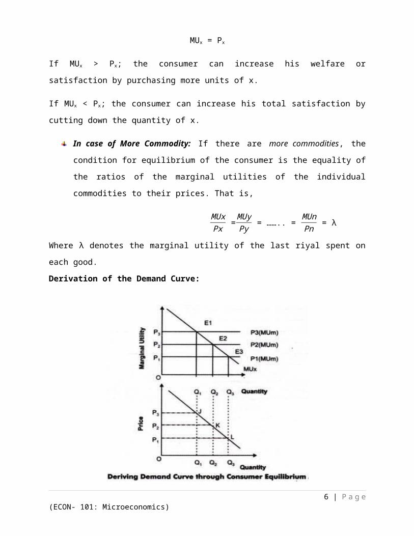
table-

UnitsMUxPx

MUyPy

1 20/2 = 10 24/3 = 82 18/2 = 9 21/3 = 73 16/2 = 8 18/3 = 64 14/2 = 7 15/3 = 55 12/2 = 6 9/3 = 36 10/2 = 5 3/3 = 1

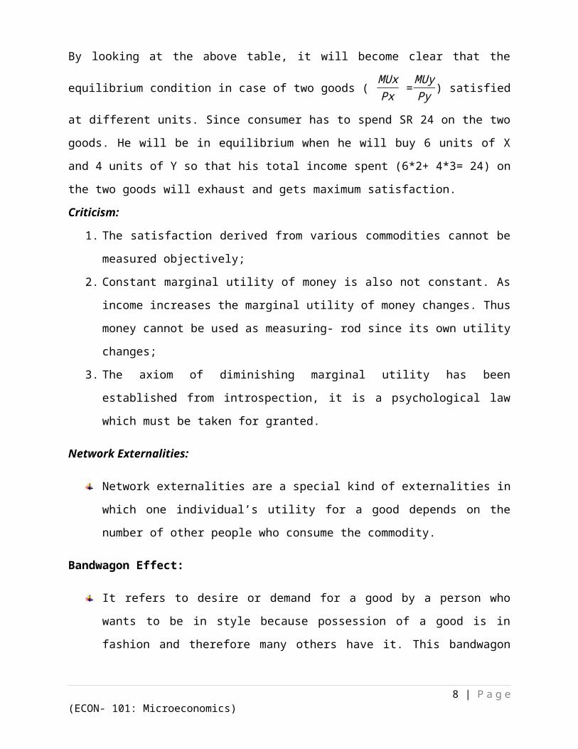
By looking at the above table, it will become clear that the equilibrium condition in case of two

goods ( MUxPx =

MUyPy ) satisfied at different units. Since consumer has to spend SR 24 on the two

goods. He will be in equilibrium when he will buy 6 units of X and 4 units of Y so that his total

income spent (6*2+ 4*3= 24) on the two goods will exhaust and gets maximum satisfaction.

Criticism:

1. The satisfaction derived from various commodities cannot be measured objectively;

2. Constant marginal utility of money is also not constant. As income increases the marginal

utility of money changes. Thus money cannot be used as measuring- rod since its own

utility changes;

3. The axiom of diminishing marginal utility has been established from introspection, it is a

psychological law which must be taken for granted.

Network Externalities:

Network externalities are a special kind of externalities in which one individual’s utility

for a good depends on the number of other people who consume the commodity.

Bandwagon Effect:

It refers to desire or demand for a good by a person who wants to be in style because

possession of a good is in fashion and therefore many others have it. This bandwagon

effect is the important objective of marketing and advertising strategies of several

manufacturing companies.

It is an example of positive network externality in which the quantity demanded of a

good that an individual buys increases in response to the increase in the quantity

purchased by other individuals. Bandwagon effect makes the demand curve elastic.


Snob Effect:

It refers to the desire to possess a unique commodity having a prestige value. It works

quite contrary to the bandwagon effect. It is an example of negative network externality.

Snob effect makes the demand curve less elastic (inelastic).

Ordinal Utility Approach: Indifference Curve Analysis- I

The cardinal approach has been severely criticised for its assumptions. On this

background F. Y. Edgeworth (1881), Vilfredo Pareto (1906), E. E. Slutsky (1915)

derived consumer’s equilibrium with the help of indifference curves.

Ultimately J. R. Hicks and R.G.D. Allen presented a scientific treatment to the consumer

theory on the basis of ordinal utility, graphically represented by indifference curves.

Indifference Curve:

It shows various combinations of the two goods which give equal satisfaction or utility to

the consumer.

An indifference curve is the locus of points which yield the same utility (level of

satisfaction) to the consumer, so that he is indifferent as to the particular combination he

consumes.

Combinations of goods situated on an indifference curve yield the same utility.

Combinations of goods lying on a higher indifference curve yield higher level of

satisfaction and are preferred.

Indifference map:

An indifference map shows all the indifference curves which rank the preferences of the

consumer.

Indifference Curve Indifference Map


The indifference curve theory is based on these assumptions:

1. Rationality;

2. Ordinality;

3. Diminishing Marginal Rate of Substitution;

4. Consistency and transitivity of choice;

Properties/ features of the indifference curves:

1. Downward sloping to the right (an indifference curve has a negative slope, which denotes

that if the quantity of one commodity (y) decreases, the quantity of the other (x) must

increase, if the consumer is to stay on the same level of satisfaction).

2. Indifference curves are convex to the origin. It means the slope of an indifference curve

(marginal rate of substitution of X for Y or MRSXY) decreases. This implies that the

commodities can substitute one another, but are not perfect substitutes. If the

commodities are perfect substitute the indifference curve becomes a straight line with

negative slope. If the commodities are complements the indifference curve takes the

shape of a right angle.


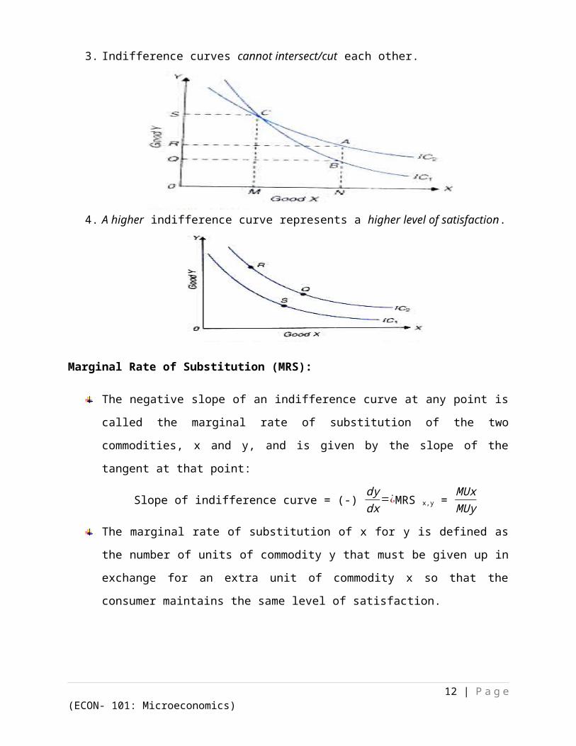
3. Indifference curves cannot intersect/cut each other.

4. A higher indifference curve represents a higher level of satisfaction.

Marginal Rate of Substitution (MRS):

The negative slope of an indifference curve at any point is called the marginal rate of

substitution of the two commodities, x and y, and is given by the slope of the tangent at

that point:

Slope of indifference curve = (-) dydx

=¿MRS x,y = MUxMUy

The marginal rate of substitution of x for y is defined as the number of units of

commodity y that must be given up in exchange for an extra unit of commodity x so that

the consumer maintains the same level of satisfaction.


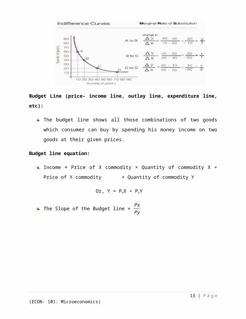
Budget Line (price- income line, outlay line, expenditure line, etc):

The budget line shows all those combinations of two goods which consumer can buy by

spending his money income on two goods at their given prices.

Budget line equation:

Income = Price of X commodity × Quantity of commodity X + Price of Y commodity

× Quantity of commodity Y

Or, Y = PxX + PyY

The Slope of the Budget line = PxPy


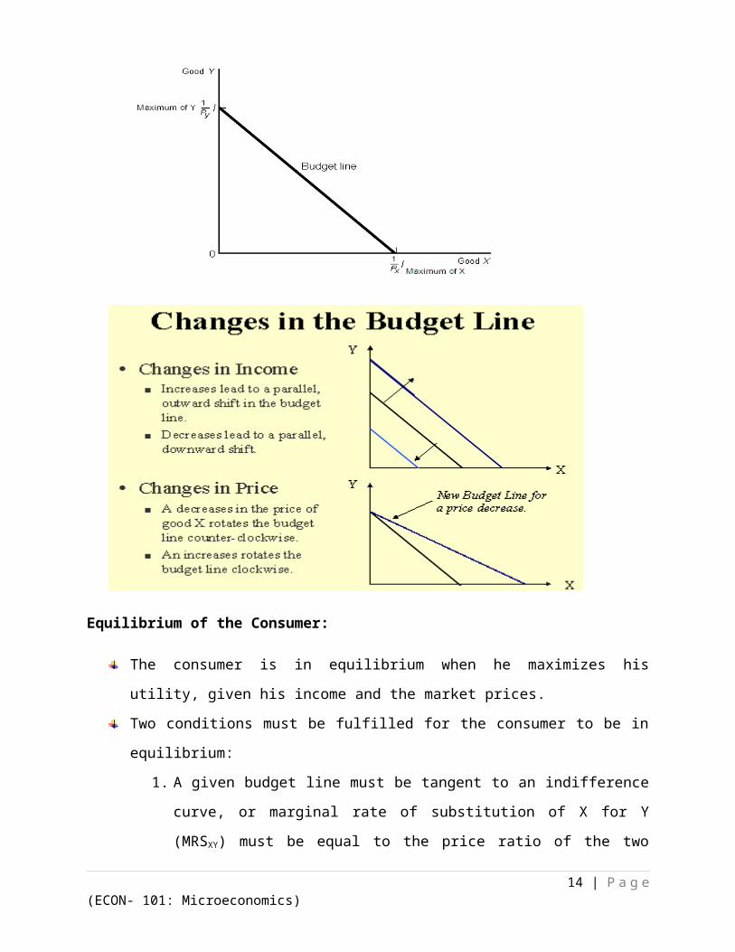
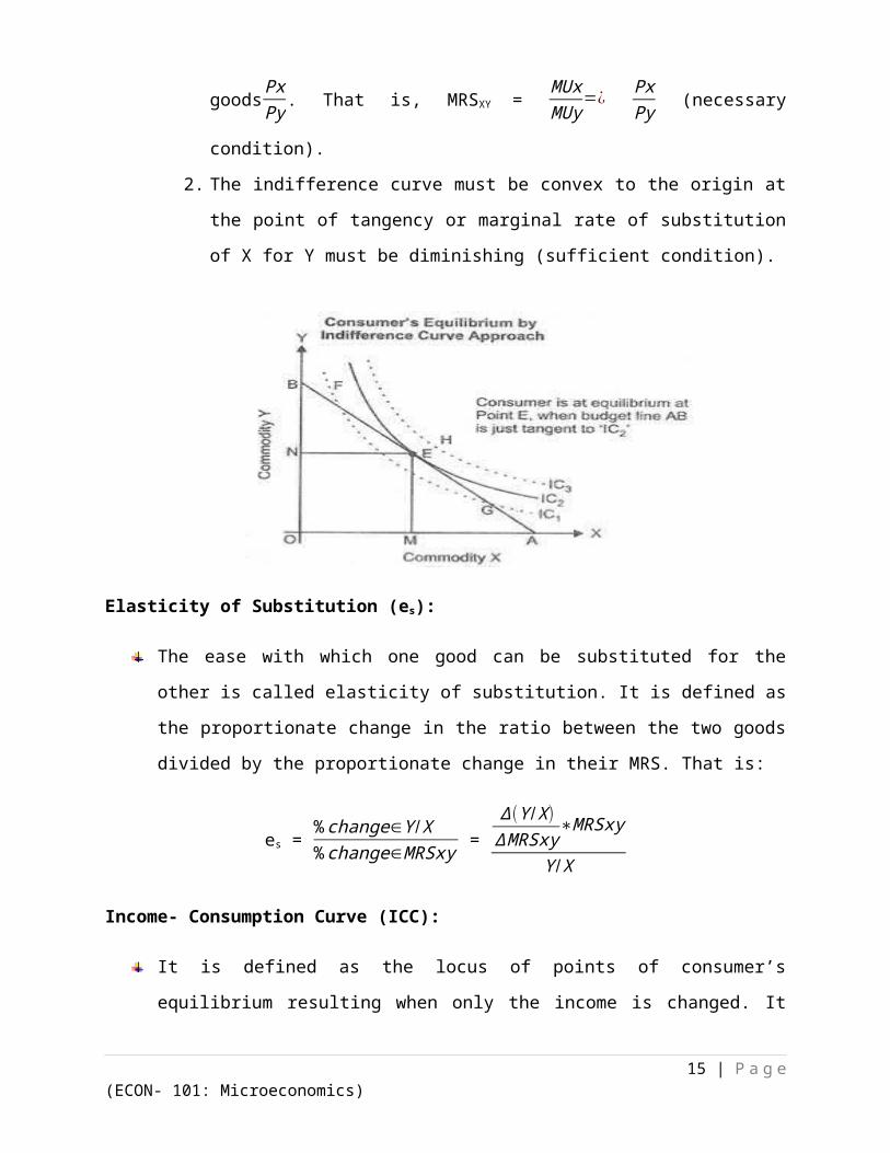
Equilibrium of the Consumer:

The consumer is in equilibrium when he maximizes his utility, given his income and the

market prices.

Two conditions must be fulfilled for the consumer to be in equilibrium:

1. A given budget line must be tangent to an indifference curve, or marginal rate of

substitution of X for Y (MRSXY) must be equal to the price ratio of the two goods

PxPy . That is, MRSXY = MUx

MUy=¿ Px

Py (necessary condition).

2. The indifference curve must be convex to the origin at the point of tangency or

marginal rate of substitution of X for Y must be diminishing (sufficient

condition).


Elasticity of Substitution (es):

The ease with which one good can be substituted for the other is called elasticity of

substitution. It is defined as the proportionate change in the ratio between the two goods

divided by the proportionate change in their MRS. That is:

es = % change∈Y / X% change∈MRSxy =

∆ (Y / X )∆ MRSxy

∗MRSxy

Y / X

Income- Consumption Curve (ICC):

It is defined as the locus of points of consumer’s equilibrium resulting when only the

income is changed. It shows the effect of a change in the money income of the consumer

on the quantity of the goods bought, ceteris paribus.

At each point of ICC slope of indifference curve is equal to slope of budget line.


Normal goods: Goods for which changes in consumption are positively related to changes in

income are said to be normal or superior goods.

Inferior goods: In case of inferior goods, consumption falls with increase in income.

Engel’s Curve:

Engel’s curve shows the amount of a commodity that the consumer will purchase per unit

of time at various levels of income.

This curve was developed by German Statistician, Christian Lorenz Ernst Engel.

This curves are derived from income- consumption curves.

Price Consumption Curve (PCC):

It shows the effect of a change in price of a commodity on the quantity of it bought,

ceteris paribus.

It is defined as the locus of points of consumer’s equilibrium resulting when only the

price of good X (or the price of good Y) is changed.

At each point of the PCC slope of indifference curve is equal to slope of budget line.

PCC shows the price effect (PE).

Price effect (PE) is split into substitution effect (SE) and income effect (IE). That is, PE =

SE + IE.

The shape of PCC depends upon the directions of SE and IE.

Price Effect (PE):


A change in price of good X brings about a change in the quantity demanded of it, ceteris

paribus. This change in the quantity demanded is called price effect.

Price effect is split into two components:

1. Substitution effect (SE); and

2. Income effect (IE).

Substitution Effect (SE):

The substitution effect is the increase in the quantity bought as the price of the

commodity falls, after adjusting income so as to keep the real purchasing power of the

consumer the same before.

This adjustment in income is called compensating variation and is shown graphically by a

parallel shift of the new budget line until it becomes tangent to the initial indifference

curve.

Income Effect (IE):

It states that a change in the price of a good will bring about a change in the real income

(purchasing power) of the consumer, which in turn brings about a change in the quantity

demanded of the good.

The IE operates on the assumption that relative price of goods remains constant.

Derivation of the Demand Curve: 14 | P a g e


Consumer Surplus:

The concept of consumer surplus has been given by Marshall and Hicks.

Consumer surplus is defined as the net benefit or gain which a consumer enjoys by

consuming one market basket instead of another.

Marshallian Consumer Surplus:

The excess amount he was willing to pay but does not have to pay is called consumer

surplus.

It is based on the law of diminishing marginal utility.


Hicksian Consumer Surplus:

Prof. J. R. Hicks modified the Marshallian consumer surplus which is equal to the area

between the demand curve and the price line.

Hicksian consumer surplus is equal to the vertical distance between the indifference

curves.

Hicksian consumer surplus is better as it is based on neither cardinal measurement of

utility nor constant marginal utility of money.

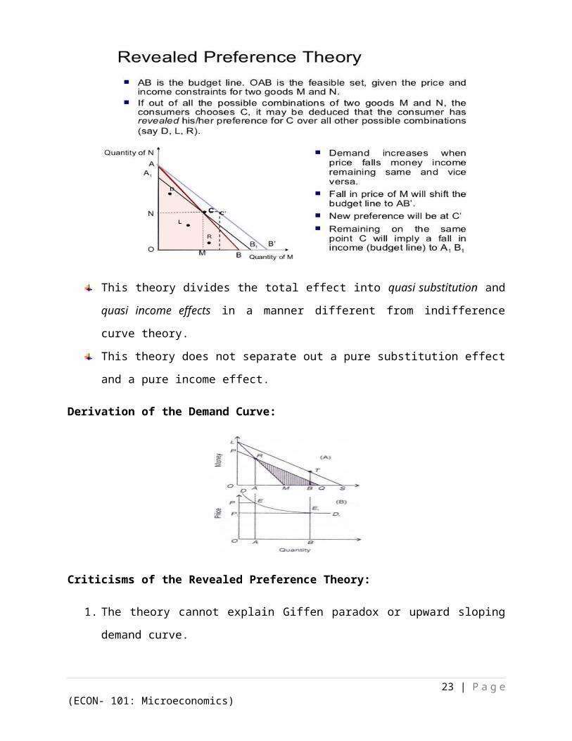
Revealed Preference Theory

Meaning of Revealed Preference: When a consumer buys a commodity he reveals his

preference for it.16 | P a g e


Revealed preference theory was developed by Paul A. Samuelson in 1938. This theory

was developed as an alternative theory of demand based on observed market behaviour of

consumers.

Samuelson has criticised the marginal utility and indifference curve theories for studying

consumers’ behaviour, by describing them as introspective.

Samuelson rejected the weak ordering hypothesis given by Hicks and built up his theory

on strong ordering hypothesis.

The revealed preference theory is also known as behaviouristic- ordinalist approach.

It is behaviouristic because it relies on actual market behaviour; and ordinalist because it

assumes utility as an ordinal concept.

This theory derives the law of demand in a direct and simple manner.

Samuelson deduced the fundamental theorem of consumption which states that demand

for a commodity and its price are inversely related provided income elasticity of demand

is positive.

The revealed preference theory is based on two axiom:

1. It states that from any set of alternatives, the consumer makes a choice; and

2. It states that if A is chosen from a set of alternatives that includes B (which is

different from A), then any set of alternating from which B is chosen must not

contain A.

Assumption of Revealed Preference Theory:

1. Rationality;

2. Consistency;


3. Transitivity; and

4. Axiom of revealed preference.

This theory divides the total effect into quasi substitution and quasi income effects in a

manner different from indifference curve theory.

This theory does not separate out a pure substitution effect and a pure income effect.

Derivation of the Demand Curve:

Criticisms of the Revealed Preference Theory:

1. The theory cannot explain Giffen paradox or upward sloping demand curve.

2. It provides a direct way to the derivation of the demand curve.

Review QuestionsI. Multiple Choice Questions:

1. Utility of every additional unit is called-18 | P a g e


a. Marginal utility b. Total utilityc. Average utility d. None of these.

2. MUn is equal to-

a. TUn + TUn-1 b. TUn – TUn-1

c. TUn – TUn+1 d. TUn + TUn+1

3. When total utility reaches at maximum marginal utility becomes

a. Positive b. Negative c. Zero d. All may be possible.

4. The cardinalist school postulated that utility can

a. Be measured b. Not be measuredc. Both a and b may possible d. None.

5. The law of equi- marginal utility is also known as-

a. Gossen’s first law b. Gossen’s second lawc. Gossen’s third law d. None of the above.

6. Gossen, Jevons, Walras and Marshall are related to-

a. Cardinal school b. Ordinal schoolc. Both a & b d. None of the above.

7. The ordinalist school postulated that utility is

a. Measurable b. Not measurablec. Both a & b may be possible d. None.

8. Pareto, W. E. Johnson, E. E. Slutsky, J. R. Hicks and R.G.D. Allen are the main economists related to-

a. Cardinal school b. Ordinal schoolc. Both school d. None of the above.

9. As the consumer consumes more of a commodity, the utility of every additional unit (MU) consumed diminishes. This is-

a. Law of diminishing marginal utility

b. Equi- marginal utility


c. Indifference curve theory d. Revealed preference theory.

10. The condition for equilibrium of the consumer is-

a.MUxPx =

MUyPy b.

MUxMUy =

PyPx

c. a&b d. MUx= MUy

11. The cardinal utility approach is based on-

a. Rationality b. Constant marginal utility of money

c. Diminishing marginal utility d. All of the above.

12. What is/ are true for indifference curves-

a. Indifference curve slopes downward to the right;b. Indifference curves are convex to the origin;c. A higher indifference curve represents a higher level of satisfaction;d. All of the above are correct.

13. The convexity of indifference curve is due to-

a. Diminishing MRS b. Increasing MRSc. Constant MRS d. None.

14. The slope of indifference curve is known as-a. Marginal Rate of Substitution; b. Marginal Utility;c. Elasticity of Substitution; d. None.

15. In indifference curve analysis, the consumer will be in equilibrium when-

a. A given budget line must be tangent to an indifference curve

b. The indifference curve must be convex to the origin at the point of tangency

c. Both a & b d. None of the above.

16. The ease with which one good can be substituted for the other is called-

a. Elasticity of substitution; b. Marginal rate of substitution;c. Substitution effect; d. None of the above.

17. A change in price of good X brings about a change in the quantity demanded of it, ceteris paribus. This change in the quantity demanded is called-


a. Price effect; b. Income effect;c. Substitution effect; d. None.

18. The increase in the quantity bought as the price of the commodity falls, after adjusting income so as to keep the real purchasing power of the consumer the same before is known as-


19. A change in the price of a good will bring about a change in the real income (purchasing power) of the consumer, which in turn brings about a change in the quantity demanded of the good is called-


20. Price effect is equal to-

a. Substitution effect; b. Income effect;c. a+b d. a-b.

21. Revealed preference theory was developed by-

a. Paul A. Samuelson b. J. R. Hicksc. Marshall d. Adam Smith

22. Revealed preference theory is based on-

a. Weak ordering b. Strong orderingc. Both a & b d. None.

23. Indifference curve analysis is based on-

a. Weak ordering b. Strong orderingc. Both a & b d. None.

Q 1 2 3 4 5 6 7 8 9 10

11

12

13

14

15

16

17

18

19

20

21

22

23

A a b c a b a b b a c d d a a c a a c b c a b a


II. Matching Test:

Match- I Match- IIA. Cardinal Utility Analysis a. P. A. SamuelsonB. Indifference Curve Analysis b. A. MarshallC. Concept of consumer surplus c. Hicks & AllenD. Revealed preference theory d. Marshall & Hicks

Match- I A B C DMatch- II b c d a

Match- I Match- IIA. Slope of indifference curve a. MRS x,y =

MUxMUy

B. Slope of budget line b.PxPy

C. Consumer’s equilibrium c.MUxMUy

= PxPy

D. MUn d. TUn – TUn-1

Match- I A B C DMatch- II a b c d

III. Write T for True and F for False against each statement:

1. Utility means want satisfying power of a commodity.2. A change in total utility resulting from a one unit change in the consumption of a

commodity at particular point of time is called marginal utility.3. Total utility is the sum of marginal utility.

4. MU = TUn + TUn-1

5. When total utility reaches at maximum marginal utility becomes zero.6. The cardinalist schoolstates that utility cannot be measured.

7. The law of diminishing marginal utility is known as Gossen’s first law.8. The law of equi- marginal utility is known as Gossen’s second law.9. The ordinalist schoolstates that utility is measurable.10.The Law of diminishing marginal utility states that as the consumer consumes more of a

commodity, the utility of every additional unit (MU) consumed diminishes.11.The principle of equi- marginal utility states that the consumer will distribute his money

income in such a way that the utility derived from the last Saudi Riyal spent on each good is equal. In other words the consumer is in equilibrium position when marginal utility of money spent on each good is same.


12.Bandwagon effectis an example of negative network externality.13. Snob effect is an example of positive network externality.14.A higher indifference curve represents a higher level of satisfaction.15. Indifference curves are convex to the origin.16.Price effect is split into two components- substitution effect and income effect.17.Revealed preference theory was developed by J. R. Hicks in 1938.

Q 1 2 3 4 5 6 7 8 9 10 11 12 13 14 15 16 17A T T T F T F T T F T T F F T T T F

IV. Questions with Answers:

Ques: What is utility?

Ans: want satisfying power of a commodity is called utility.

Ques: What is total utility and marginal utility?

Ans: Total utility: The sum of total satisfaction which a consumer receives by consuming various units of the same commodity.

Marginal Utility: It refers as utility of every additional unit of the consumed or it can be can be defined as a change in total utility resulting from a one unit change in the consumption of a commodity at particular point of time.

Ques: What are the relationships between total utility and marginal utility?

Ans: Relationship between Total Utility and Marginal Utility:

Total Utility Marginal UtilityAs we consume more goods total utility increases but diminishing rate.

As we consume more goods marginal utility diminishes.

When total utility reaches at maximum Marginal utility becomes zero.When total utility declines Marginal utility becomes negative.

Ques: What is law of diminishing marginal utility?

Ans: The Law of diminishing marginal utility states that as the consumer consumes more of a commodity, the utility of every additional unit (MU) consumed diminishes.

Ques: What is the law/ principle of equi- marginal utility?


Ans: The principle of equi- marginal utility states that the consumer will distribute his money income in such a way that the utility derived from the last Saudi Riyal spent on each good is equal. In other words the consumer is in equilibrium position when marginal utility of money spent on each good is same.

Ques: What is/are the condition(s) for consumer equilibrium in cardinal approach?

Ans: In case of Single Commodity:

MUx = Px

In case of More Commodity:

MUxPx =

MUyPy = …….. =

MUnPn = λ

Where λ denotes the marginal utility of the last riyal spent on each good.Ques: What are Bandwagon and Snob effects?

Ans: Bandwagon Effect: It refers to desire or demand for a good by a person who wants to be in style because possession of a good is in fashion and therefore many others have it. It is an example of positive network externality. Bandwagon effect makes the demand curve elastic.

Snob Effect: It refers to the desire to possess a unique commodity having a prestige value. It works quite contrary to the bandwagon effect. It is an example of negative network externality. Snob effect makes the demand curve less elastic (inelastic).

Ques: What is indifference curve?

Ans: An indifference curve is the locus of points which yield the same utility (level of satisfaction) to the consumer, so that he is indifferent as to the particular combination he consumes. It shows various combinations of the two goods which give equal satisfaction or utility to the consumer.

Ques: What are the main features/properties of indifference curves?

Ans: The main features/properties of indifference curves are-

1. Downward sloping to the right;2. Indifference curves are convex to the origin;3. Indifference curves cannot intersect/cut each other; and4. A higher indifference curve represents a higher level of satisfaction.

Ques: What do you mean by marginal rate of substitution (MRS)?

Ans: The marginal rate of substitution of x for y is defined as the number of units of commodity y that must be given up in exchange for an extra unit of commodity x so that the consumer maintains the same level of satisfaction.


The negative slope of an indifference curve at any point is called the marginal rate of substitution of the two commodities, x and y, and is given by the slope of the tangent at that point:

Slope of indifference curve = (-) dydx

=¿MRS x,y = MUxMUy

Ques: What are the conditions for consumer’s equilibrium in indifference curve analysis?

Ans: The consumer is in equilibrium when he maximizes his utility, given his income and the market prices. Two conditions must be fulfilled for the consumer to be in equilibrium:

1. A given budget line must be tangent to an indifference curve, or marginal rate of substitution of X for Y (MRSXY) must be equal to the price ratio of the two goodsPxPy . That is, MRSXY =

MUxMUy

= PxPy (necessary condition).

2. The indifference curve must be convex to the origin at the point of tangency or marginal rate of substitution of X for Y must be diminishing (sufficient condition).

Ques: What is elasticity of substitution?

Ans: The ease with which one good can be substituted for the other is called elasticity of substitution. It is defined as the proportionate change in the ratio between the two goods divided by the proportionate change in their MRS. That is:

es = % change∈Y / X% change∈MRSxy =

∆ (Y / X )∆ MRSxy

∗MRSxy

Y / X

Ques: What is income- consumption curve (ICC)?

Ans: It is defined as the locus of points of consumer’s equilibrium resulting when only the income is changed. It shows the effect of a change in the money income of the consumer on the quantity of the goods bought, ceteris paribus. At each point of ICC slope of indifference curve is equal to slope of budget line.

Ques: What is Engel’s curve?

Ans: Engel’s curve shows the amount of a commodity that the consumer will purchase per unit of time at various levels of income. This curve was developed by German Statistician, Christian Lorenz Ernst Engel. This curves are derived from income- consumption curves.

Ques: What is price consumption curve (PCC)?

Ans: It is defined as the locus of points of consumer’s equilibrium resulting when only the price of good X (or the price of good Y) is changed.


Ques: What is price effect? substitution effect and income effect?

Ans: Price Effect (PE): A change in price of good X brings about a change in the quantity demanded of it, ceteris paribus. This change in the quantity demanded is called price effect.

Ques: What is substitution effect?

Ans: Substitution Effect (SE): The substitution effect is the increase in the quantity bought as the price of the commodity falls, after adjusting income so as to keep the real purchasing power of the consumer the same before.

Ques: What is income effect?

Ans: Income Effect (IE): It states that a change in the price of a good will bring about a change in the real income (purchasing power) of the consumer, which in turn brings about a change in the quantity demanded of the good.

Ques: What do you understand by consumer surplus?

Ans: The concept of consumer surplus has been given by Marshall and Hicks. Consumer’s Surplus is the simply difference between the price one is willing to pay the price one actually pays for particular product.

Ques: What is Marshallian consumer surplus?

Ans: The excess amount he was willing to pay but does not have to pay is called consumer surplus. It is based on the law of diminishing marginal utility.

Ques: What is Hicksian consumer surplus?

Ans: Hicksian consumer surplus is equal to the vertical distance between the indifference curves.

Ques: What is revealed preference theory?

Ans: When a consumer buys a commodity he reveals his preference for it. This theory was developed by Paul A. Samuelson in 1938. This theory was developed as an alternative theory of demand based on observed market behaviour of consumers. Samuelson rejected the weak ordering hypothesis given by Hicks and built up his theory on strong ordering hypothesis. The revealed preference theory is also known as behaviouristic- ordinalist approach.

*****


fac.ksu.edu.safac.ksu.edu.sa/.../default/files/6._consumers_behaviour.docx · Web viewThe taste and...

Documents

Transcript of fac.ksu.edu.safac.ksu.edu.sa/.../default/files/6._consumers_behaviour.docx · Web viewThe taste and...