ARTICLE IN PRESS

Nuclear Instruments and Methods in Physics Research A 607 (2009) 544–553

Contents lists available at ScienceDirect

Nuclear Instruments and Methods inPhysics Research A

0168-90

doi:10.1

� Corr

E-m

journal homepage: www.elsevier.com/locate/nima

Ground calibration of the Chandrayaan-1 X-ray Solar Monitor (XSM)

L. Alha a,�, J. Huovelin a, K. Nygard b, H. Andersson c, E. Esko a, C.J. Howe d, B.J. Kellett d, S. Narendranath g,B.J. Maddison d, I.A. Crawford e, M. Grande f, P. Shreekumar g

a Observatory, P.O. Box 14, FI-00014 University of Helsinki, Finlandb Division of X-ray Physics, Department of Physics, P.O. Box 64, FIN-00014 University of Helsinki, Finlandc Oxford Instruments Analytical, P.O. Box 85, FIN-02631 Espoo, Finlandd Rutherford Appleton Laboratory, Chilton, Didcot OX11 0QX, UKe School of Earth Sciences, Birkbeck College, London, UKf Institute of Mathematical and Physical Sciences, University of Wales, Aberystwyth, Ceredigion SY23 3BZ, UKg Space Astronomy and Instrumentation Division, ISRO Satellite Centre, Bangalore 560017, India

a r t i c l e i n f o

Article history:

Received 5 June 2009

Accepted 24 June 2009Available online 1 July 2009

Keywords:

X-ray detectors

Calibration

02/$ - see front matter & 2009 Elsevier B.V. A

016/j.nima.2009.06.049

esponding author. Tel.: +358 9 19121772; fax

ail address: alha@mappi.helsinki.fi (L. Alha).

a b s t r a c t

The Chandrayaan-1 XSM ground calibrations are introduced. The aim of these calibrations was to

characterize the performance of XSM, which enables a reliable spectral analysis with the solar X-ray

data. The calibrations followed an improved procedure based on our experience from the SMART-1 XSM.

The most important tasks in the calibrations were determination of the energy resolution as a function

of the photon energy and mapping of the detector sensitivity over the FoV (Field of View) of the sensor.

The FoV map was needed to determine the obscuration factor corresponding to various pointings with

respect to the Sun. We made also a sensitivity comparison test between the Chandrayaan-1 XSM FM

(Flight Model) and SMART-1 XSM FS (Flight Spare). The aim of this test was to link the new XSM

performance to a performance of an already known and tested former instrument. We also performed a

simple test to determine the pile up performance, and one specific test tailored for the operation of the

new version of XSM. Also the first experiences on the in-flight operation are briefly described.

& 2009 Elsevier B.V. All rights reserved.

1. Introduction

A new XSM (X-ray Solar Monitor) began to operate on boardthe Indian Chandrayaan-1 space craft. This first Indian lunarmission was launched on the 22 October 2008. The observationaltask of this new XSM was to observe the solar X-ray emission,while the C1XS (Chandrayaan-1 X-ray Spectrometer) instrumentwas designed to measure the fluorescence emission from theMoon soil induced by the solar X-ray emission [1]. Chandrayaan-1S/C (Space Craft) has by now reached its almost circular polarorbit about 200 km above the surface of the Moon.

This new XSM differs from its predecessor SMART-1 XSM [2] inthree ways [3]. Firstly, the low energy sensitivity was enhanced bya thinner Be-filter having a thickness of 13mm instead of 27mm,which was used in SMART-1 XSM. Secondly, the area of the goldenaperture stop hole is about 18 times smaller, to cover a widerdynamical range with respect to higher count rates during M andX-level flares. Thirdly, the sensor electronics are also equippedwith a less noisy FET transistor, compared to the former XSM. All

ll rights reserved.

: +358 9 19122952.

filter and detector dimensions, FoV (Field of View) geometry andtechnical performance values have been compiled into Table 1.

2. Ground calibrations

XSM calibrations were carried out during June 2007 in theX-ray laboratory at the University of Helsinki, Department ofPhysical Sciences. The X-ray laboratory has a vacuum chamberattached with a titanium X-ray tube. The lowest pressure obtainedwith the present two-phase rotary vane vacuum pump was4 mbar. The inner diameter of the chamber was 630 mm and thefree working height was 300 mm. The chamber consisted of anadjustable table enabling 3D-movements of the specimen. Therewas also a rotating goniometer inside the chamber enabling thestudy of FoV sensitivity at different roll and off-axis angles. Thevacuum chamber allowed measurements at soft X-ray rangeðEr5 keVÞ. The photon energy of 5 keV is a practical low energylimit, when making measurements in a free air. The primary X-raysource of the calibration setup was a sealed and air-cooledTi-anode miniature soft X-ray tube (Oxford X-ray TechnologiesInc., model XTF-5011). This X-ray tube consists of a Be windowhaving a thickness of 75mm. This limits the usable soft X-rayoutput energies to above 1.0 keV. The tube high voltage and

ARTICLE IN PRESS

L. Alha et al. / Nuclear Instruments and Methods in Physics Research A 607 (2009) 544–553 545

current were controlled manually with an accuracy of 0.1 kV (max50 kV), and 1mA (max 1 mA). There was also an 55Fe source foroperational testing, which enabled application of emission line of5.9 and 6.4 keV in calibrations. The data acquisition was controlledwith a special commercial software dedicated to laboratoryanalysis, running in the PC workstation under Linux operatingsystem. This same software controlled the movements of thespecimen. X-ray spectra were collected with a 2028 channel ISA-bus MCA (Multi-Channel Analyzer) card.

2.1. Determination of the detector energy resolution as a function of

a photon energy

Two different fluorescence samples and one 55Fe emitter wereused as emission sources. The first fluorescence sample was madeof compressed powder mixtures of Al, Ca and Cu. The secondsample was made of pure Pb plate. Both samples were illuminatedwith a titanium X-ray tube and the fluorescence emission fromthe samples was measured with the specimen. The specimen wasalso illuminated with the 55Fe source in advance to get two moreemission lines in the data. Both of the fluorescence samples weremeasured at five different detector PIN (Positive IntrinsicNegative) diode temperatures, 0, �5, �10, �15 and �20 3C. Theintegration time per spectrum with the Pb-sample was 2 h. Therespective integration time with the AlCaCu-sample was 1 h.Tables 2 and 3 include a list of line energies used in these energyresolution measurements. The spectra of both samples were alsoanalyzed to determine the respective gains, offsets and linecentroids. The results of this test are shown in Fig. 1. Similar plotsof the fluorescence spectra used in this test can be found inSection 2.4. (These plots exclude the Mn-lines from the 55Fe,which were not used in the comparison test.)

Table 2Line centroids, energy resolutions, gains and offsets derived from the fluorescence line

Temp. ð3CÞ Al Ka Ca Ka Ti Ka

Cent FWHM Cent FWHM Cent

þ0 73.36 0.163 180.92 0.192 220.

�5 72.60 0.180 179.80 0.176 219.3

�10 72.68 0.155 180.69 0.174 220.

�15 72.10 0.151 179.91 0.174 219.3

�20 115.52 0.197 218.79 0.171 511.8

Table 1XSM filter and detector dimensions.

Detector dimensions and performance Nominal values

Detector thickness, Si 500:0mm

Si dead layer thickness 0:01mm

Al-filter+contact thickness, Al 0:60mm

Polyimide filter 0:25mm

Be-filter thickness 13:0mm

Effective aperture stop diameter, ddet 0.379 mm

Aperture diameter 4.70 mm

Detector–aperture distance 2.00 mm

Field of View cone angle radius 523

Number of channels 512

Energy range 1.2–20.0 keV

Energy resolution (BOL) 200 eV at 6 keV

Pile up 3% at 20 000 cps

2.2. FoV (Field of View) sensitivity

The sensitivity of the detector FoV was derived as a function oftwo angles. These were the off-axis angle y and the roll angle r.The parameter y is the angular distance between the Sun and thedetector optical axis. The (azimuthal) roll angle r is related to theFoV in a way shown in Fig. 3. The detector FoV corresponds to acircle having an angular radius of 523 in the celestial sphere. Onthe circular orbit 200 km above the Moon, the angular velocity ofthe Sun moving in the FoV is about 33=min. Hence the detectorsensitivity must be known with an accuracy of 13 throughout inthe FoV as a function of r and y. The change of the sensitivity iscaused by the dependence of the projected detector area and theshadow cast by the aperture collimator on the detector active areaon the position of the light source (the Sun) in the FoV. Hence, thesensitivity is a function of r and y.

The sensitivity map of the FoV was generated by illuminatingthe detector at different angles with a constant white beam of aTi-anode X-ray tube. A detailed description of this procedure canbe found in paper [2]. The outcome of this measurement is a two-dimensional array containing obscuration factors correspondingto angle pairs of r and y, which determine the position of the Sunin the detector FoV. The contour plot of this obscuration factorarray is shown in Fig. 2. The test setup information related to theFoV sensitivity map is listed in Table 4 (see Figs. 2 and 3).

2.3. Determination of the aperture stop diameter

The most crucial task in determining the sensitivity of amonolithic semiconductor detector is to quantify the exact size ofthe detector active area. This area is dictated by the stop holeaperture stop, which was machined manually by a drill bit havinga nominal diameter of 0.35 mm. The edge of the aperture stop holewas found to deviate from an ideal circle by analyzing thephotographs taken from under and above the machined aperturestop with a microscope. Fig. 4 illustrates the scenery taken fromabove the aperture stop, i.e. from the direction of the light source.As can be seen, the hole edge geometry shown in Fig. 4 is quitedifficult to determine accurately. Luckily, the manufacturer hadincluded a dimensional reference scale object (i.e. a 0.35 mm drillbit) in these two jpg-formatted photos. Thus we could do aquantitative image analysis to derive the effective diameter of thedrilled aperture stop hole. First we imported the photos into XFIG(a vector based drawing program running under Linux) S/W, inwhich we added a white color circle having an equal diameter asthe drill bit. Hence, we were able to determine the metricdimensional scale of the photograph, i.e. pixel versus physical unitscale. The resulting figure was exported into an FITS-formatted filefrom the XFIG program and the pixel information was analyzedwith the aid of the IDLTM S/W in three different colors, R (red), G(green) and B (blue). The total number of pixels corresponding tothe free entrance area of the aperture hole was calculated in threepixel colors. We obtained six different values for the hole areas in

s of AlCaCu powder mixture sample.

Cu Ka Gain Offset

FWHM Cent FWHM

22 0.202 392.53 0.230 0.0206 �0.022

0 0.191 390.87 0.219 0.0206 �0.012

47 0.185 393.26 0.204 0.0205 �0.003

9 0.181 392.20 0.197 0.0205 +0.008

7 0.231 612.02 0.225 0.0206 �0.025

ARTICLE IN PRESS

Table 3Line centroids, energy resolutions, gains and offsets derived from the fluorescence lines of Pb plate sample.

Temp. ð3CÞ Pb Ma Ti Ka Pb La Pb Lb Gain Offset

Cent FWHM Cent FWHM Cent FWHM Cent FWHM

þ0 117.64 0.240 221.05 0.197 514.53 0.258 615.30 0.268 0.0206 �0.062

�5 117.42 0.220 221.55 0.196 516.28 0.251 617.16 0.254 0.0205 �0.051

�10 116.97 0.204 221.08 0.183 515.98 0.210 616.89 0.236 0.0205 �0.040

�15 116.15 0.204 220.09 0.184 514.41 0.233 615.39 0.216 0.0205 �0.026

�20 115.52 0.197 218.79 0.171 511.87 0.231 612.02 0.225 0.0206 �0.025

Fig. 1. XSM energy resolution as a function of photon energy at five different PIN

temperatures.

Table 4The test setup parameters applied in the FoV sensitivity calibration.

Source Ti anode X-ray tube

Tube voltage 12 keV

Tube current 0.005 mA

Slit size 10 mm� 10 mm

PIN temp. �15 3C

Chamber pressure 4 mbar

Extra filters 4 capton foils

Total count rate 3.0 kcps

Count rate (7–9 keV) 0.4 kcps

Off-axis step 13

Number of steps per scan 111

Number of scans 4

Scan 1 roll angles 03; . . . ;1803

Scan 2 roll angles 453; . . . ;2253

Scan 3 roll angles 903 ; . . . ;2703

Scan 4 roll angles 1353; . . . ;3153

Fig. 2. XSM FoV sensitivity map describing the obscuration factor.

L. Alha et al. / Nuclear Instruments and Methods in Physics Research A 607 (2009) 544–553546

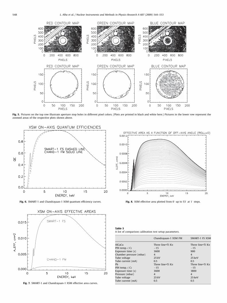
total (three colors below and three colors above). The outcome ofthis photographic analysis yielded an effective diameter 0.379 mmfor the Au aperture stop. The analyzed photographs illustratingthe aperture stop hole in three different colors are shown in Fig. 5.The top row figures were generated with XFIG S/W. The annuliaround the aperture holes were drawn in white to remove allpixels misleading the analysis. The plots in the lower row in Fig. 5illustrate a more detailed and zoomed in areas of the manipulatedphotos in the respective pixel colors. (Coloring in Fig. 5 is gray.)

2.4. Comparison calibration

From the known size of Au aperture stop hole, one candetermine the effective on-axis area for the detector, i.e. an ARF

(Ancillary Response File) required in the spectral analysis. The QE(Quantum Efficiency) curves of the Chandrayaan-1 XSM FM andSMART-1 XSM FS are shown in Fig. 6. As can be seen, the QE-curveof the Chanrayaan-1 XSM is bit better at the low energy side dueto the thinner Be-window. The plots representing the effectiveareas are shown in Fig. 7. The effective area of the SMART-1 XSMFS is greater due to the bigger aperture stop hole of 1.5 mm. Fig. 8illustrates the Chanrayaan-1 XSM FM effective area calculated atthe roll angle direction of 03.

In this comparison calibration, the SMART-1 XSM FS andChandrayaan-1 XSM FM detectors were both tested under sameconditions. The test setup parameters are given in Table 5. Theapplied fluorescence sources used in this test were the same asin the energy resolution determination calibration explained inSection 2.4, except for excluding the Mn lines from the 55Fe-source. The resulting fluorescent spectra are shown in Figs. 9 and10. The setup parameters related to this comparison test are givenin Table 5. The spectra were first fitted with the XSPEC S/W [4].Each applied fluorescence line was fitted and the fit parameters(KFM and KFS) denoting the line intensities were then compared.The applied lines and numerical results are listed in Table 6. Theplot in Fig. 11 illustrates the result of the comparison calibrationbetween SMART-1 XSM FS and Chandrayaan-1 XSM FM. TheSMART-1 XSM FS is an identical replica of the SMART-1 XSM FM.The latter data have been cross calibrated with the simultaneousGOES [5] (flux) data to an accuracy of about 75% during the on-axis observations. For all practical purposes, this test connectedthe Chandrayaan-1 XSM FM sensitivity to the tested performance

ARTICLE IN PRESS

135° 90°

45°

0°

315°270°

225°

XSM FRONT VIEW VS. ROLL ANGLESS

180°

Fig. 3. XSM roll angle directions related to the FoV sensitivity scanning.

Fig. 4. Aperture stop photographed with a microscope. Reference scale patterns

are drawn in the figure.

L. Alha et al. / Nuclear Instruments and Methods in Physics Research A 607 (2009) 544–553 547

of previously tested detectors with known sensitivity. Thesensitivity of the Chandrayaan-1 XSM FM matches quite wellwith the sensitivity of the SMART-1 XSM FS, which in turnrepresents the verified sensitivity of the SMART-1 XSM FM.

2.5. Pile up test

The pile up test was carried out at the facilities of themanufacturing company, i.e. at OIA (Oxford Instruments Analy-tical) in Espoo, Finland. The FM electronics box was used in this

test. The radiation source was an 55Fe emitter with two lines at 5.9and 6.5 keV. The radiation source was placed at five differentdistances from the detector to modify the recorded count rates.The closer the radiation source was to the detector, the higher wasthe count rate and the respective number of pile up counts. Thetotal count rates were calculated by adding 2E and 3E pile upcount rates with the total count rates obtained from the rest of thechannels. The 2E count rates were multiplied by a factor of twoand the 3E pile up count rates by a factor of three, which gave theintrinsic source count rates, apart from the absorption effects. Thetheoretical pile up curve shown in Fig. 12 includes the sum of the2E and 3E pile up count rates both calculated applying Poissonstatistics as shown below:

Pile up ¼ðtIÞnexpð�tIÞ

n!ð1Þ

The parameter n is 1 for the 2E and 2 for the 3E count rates. Theparameter t denotes the fast channel nominal pulse per resolutiontime of 2:0ms. The parameter I is the total count rate.

The calculated pile up for the test data yielded a fasteroperation for the fast channel, i.e. the pulse per resolution timewas only about 1:57ms. The calculated and theoretical pile upcurves are shown in Fig. 13.

The XSM front-end electronics is composed of the twodifferent channels, both recording the same incoming photons.The fast channel acts as a photon counter. As long as the timeinterval between two successive incoming photons is greater thanthe pulse per resolution time, the fast channel can record allincoming photons. The other channel, the slow channel, measuresthe energy of incoming photons. While a photon energymeasurement is going on in the slow channel, this channel isclosed for successive incoming photons. This means in practice,that all incoming photons are rejected, when a photon is under apulse height measuring in the slow channel. The time periodwhen the slow channel does not allow a new photon to enter theenergy measuring process is called dead time. In a detector whereis only one measuring channel, i.e. the slow channel, the lostsignals due to dead time must be added to the measured signalusing a Poisson statistical correction factor. This factor depends onthe duration of the dead time and measured count rate. Using afast channel readout to count the photons missed by the slowchannel replaces the mathematical dead time correction, i.e. itacts as a ‘hardware dead time corrector’. In this kind of a systemthere is no dead time. Another effect, pile up of the counts, cannotbe avoided with any realistic solution, if the incoming photoncount rate is very high.

2.6. Low energy threshold limit

The low energy limit determines the lowest applicable energychannel of the readout electronics. This limit can be changed andit is controlled by an on-board S/W parameter. The higher thislimit, the higher the lowest energy recorded. If the detector issuffering from a low energy noise, the value of this limit can beadjusted higher to reduce the low energy noise. This value shouldbe as low as possible, because the detector lower energy rangedepends on this value. If the value is set too low, the detectorgenerates phantom counts. These excess counts are related to theinterference with the fast channel operation. The aim of the lossfree counting system is to add photons rejected by the slowchannel into the final spectrum. The fast channel operation is verysensitive to any electrical interference. When the low energythreshold limit is set too low, the fast channel starts to generatephantom counts, which are added according to the loss freecounting logic to the original spectrum so that the spectrum shape

ARTICLE IN PRESS

Fig. 5. Pictures on the top row illustrate aperture stop holes in different pixel colors. (Plots are printed in black and white here.) Pictures in the lower row represent the

zoomed areas of the respective plots shown above.

Fig. 6. SMART-1 and Chandrayaan-1 XSM quantum efficiency curves.

Fig. 7. SMART-1 and Chandrayaan-1 XSM effective area curves.

Fig. 8. XSM effective area plotted from 03 up to 533 at 13 steps.

Table 5A list of comparison calibration test setup parameters.

Chandrayaan-1 XSM FM SMART-1 FS XSM

AlCaCu Three line+Ti Ka Three line+Ti KaPIN temp. ð3CÞ �15 �15

Exposure time (s) 3600 900

Chamber pressure (mbar) 4 4

Tube voltage 25 kV 25 keV

Tube current (mA) 0.5 0.5

Pb Three line+Ti Ka Three line+Ti KaPIN temp. ð3CÞ �15 �15

Exposure time (s) 3600 1800

Pressure (mbar) 4 4

Tube voltage 25 kV 25 keV

Tube current (mA) 0.5 0.5

L. Alha et al. / Nuclear Instruments and Methods in Physics Research A 607 (2009) 544–553548

ARTICLE IN PRESS

Fig. 9. Fluorescence spectrum of the powder mixture of Al, Ca and Cu.

Fig. 10. Fluorescence spectrum of the Pb plate.

Table 6Comparison calibration results between Chandrayyan-1 FM and SMART-1 FS XSM.

Line energy (keV) KFM KFS KFM=KFS

Al Ka 1.487 220.2 219.9 0.998

Pb Ma 2.345 867.4 854.4 0.985

Ca Ka 3.692 673.2 659.1 0.979

Ti Ka 4.511 142.7 146.8 1.028

Cu Ka 8.047 1192.2 1206.3 1.012

Pb La 10.50 280.1 270.8 0.967

Pb Lb 12.62 194.4 200.7 1.033

Fitting parameters KFM and KFS are derived from the XSPEC S/W. Their dimension is

photons/s/keV.

Fig. 11. Derived physical line intensity ratios.

Fig. 12. A model spectrum showing the lines used in the fit. The low energy S/W

parameter was 20 during this pile up test corresponding to the lowest applicable

channel number of 33 ð¼ 1:1 keVÞ.

Fig. 13. Theoretical and derived pile up curves.

L. Alha et al. / Nuclear Instruments and Methods in Physics Research A 607 (2009) 544–553 549

is preserved, but only the total intensity is increased. This kind ofdistortion effect is very difficult to recognize, and is therefore apotential source of serious scientific misinterpretations.

The aim of our tests were to find the lowest limit, at which theoperation is stable, i.e. the low energy noise level is insignificantand the spectra are clean of phantom counts. We made severaltests at OIA to find the optimal low energy limit for in-flightoperation of XSM. These tests were made also with the FMelectronics. Two test sequences were performed: one with amoderate count rate and the another with a high count rate. The

ARTICLE IN PRESS

Fig. 16. The measured count rate as a function of threshold parameter (moderate

count rate).

L. Alha et al. / Nuclear Instruments and Methods in Physics Research A 607 (2009) 544–553550

radiation source was the same 55Fe as used in the pile up test. Inthe first test run, the count rate was high and the operational PINtemperature was �5 3C. The operational conditions could beregarded as ‘hard’ for XSM in this first test. Eleven integrationseach containing about 10 spectra were taken at different values ofthe lower energy limit starting from the parameter value 9 andending to the value 29. Value 9 corresponds to an energy of0.4 keV and 29 corresponds to an energy of 1.7 keV. The stepinterval was 2, i.e. only the odd values were included. The secondtest run was carried out with a moderate count rate and at a lowerPIN temperature of �10 3C corresponding to the ‘nominal’operational conditions. Otherwise the second test was similar tothe first test. The plot in Fig. 14 shows the low energy noise countrates as a function of the threshold parameter. The low andconstant noise level starts at about 21 in both tests. Figs. 15 and 16illustrate the total count rates as a function of the thresholdparameter. It is clearly seen that excess counts occur in thespectra, when the parameter is less than 21, i.e. loss free countingdoes not operate properly.

The channel versus energy relation related to low energythreshold parameter values was also studied. All the spectra wereanalyzed by determining the lowest channel number containingat least a few counts. The lowest possibly recorded photon energylimits corresponding to the parameter limit values were derivedby linear fitting. The line energies used in these fits were the Si

Fig. 14. XSM low energy noise as a function of threshold parameter at two

different count rates.

Fig. 15. The measured count rate as a function of threshold parameter (high count

rate).

Fig. 17. The low energy limit plotted as a function of the threshold parameter. The

optimal parameter value 21 equals about 1.2 keV.

escape peak (4.17 keV), Mn Ka (5.9 keV), Mn Kb (6.5 keV) and 2E

pile up (11.9 keV). Hence, it was an easy task to determine therespective lowest possible channel energy corresponding to thelow energy threshold parameter. The data points are plotted inFig. 17. The fitted line in this figure represents the graphconnecting the low energy threshold parameter and the lowestmeasurable photon energy. It is worthy of pointing out that thegain and offset of XSM are also affected by the sensor box ambienttemperature and detector PIN temperature.

2.7. Calibration with in-flight source

The in-flight calibration source is an 55Fe plate attached on theshutter inner surface. This radiation source also contains a 5mmTi-foil. Hence, the calibration spectrum contains four distinctemission line, which are Ti Ka at 4.5 keV, Ti Kb at 4.9 keV, Mn Kaat 5.9 keV and Mn Kb at 6.5 keV. It was found, that the sourceintrinsic intensity was low. The aperture stop hole is about 18times smaller than it was in the SMART-1 XSM and the intrinsicsource BoL (Begin of Life) intensities were the same. Hence, thecalibration count rate was too low, yielding only about the countrate of 15 cps. With the aid of the fitted line centroids, we had tomake tests about the required number of calibration spectra,

ARTICLE IN PRESS

L. Alha et al. / Nuclear Instruments and Methods in Physics Research A 607 (2009) 544–553 551

which were needed to determine the gain and offset of XSM. Theenergy resolution was also investigated. The line centroids of Ti Kaand Mn Ka were calculated to determine the channel versusenergy relation. This required the summing of about 20 calibra-tion spectra in total to get a sufficient photon statistics. The sameamount of spectra was needed to determine the FWHM of the MnKa line. Due to the weakness of the Ti Ka line, the determinationof the FWHM of Ti Ka line required far too many spectra of 16 s, i.e.spectra with too long integration time. The longer the calibrationperiods, the less solar data obtained. If the determination of theenergy resolution of Ti Ka line failed for a sum of 20 spectra, therespective resolution could be determined iteratively. The method

Fig. 18. Gaussian fitting routine applied on the three different lines. The

resolutions stabilize after the total number of spectra used in fitting as about 60.

Fig. 19. XSM calibration line centroids, gain and offset fitted as a functi

is introduced in the equations below:

DEpffiffiffiEp

ð2Þ

DE1 ¼ DE2

ffiffiffiffiffiE1

E2

sð3Þ

The Gaussian fit tests of the three line energies are plotted in Fig.18. The horizontal axis represents the number of added calibrationspectra, which was required in the fitting of the energyresolutions. The parameter DE1 denotes the resolution of the TiKa line, while DE2 is the resolution of the Mn Ka line. The valuesfor these were DE1 ¼ 4:5 keV and DE2 ¼ 5:9 keV.

We have also studied the possibility to determine the detectoroffset and gain purely as a function of the detector PIN and sensorbox temperature. Practically this means, that no in-flight calibra-tion will be needed. The energy scale information associated tothe RMF (Redistribution Matrix File) is taken from a tablegenerated on the basis of ground calibrations the beforehand.This table includes the relation of the gain and offset as a functionof the box temperature at a constant detector PIN temperatures.The PIN temperature can be stabilized with the aid of the Peltiercooler. Both of these temperature values with time stamps arepart of the down linked telemetry data. As mentioned above,these two temperatures affect on the detector offset and gain, i.e.the determination of channel versus energy scale. We have made afits describing the relation between the box temperature and gainat two constant PIN temperature of �9 and �18 3C. XSMperformed a few long integrations with the shutter in closedposition during the commissioning phase in November 2008. Thiscalibration data were analyzed to determine the respectivepositions of line centroids of the TiKa and MnKa at severaldifferent sensor box temperatures. Those temperature were �15,�11, �3, 0 and þ4 3C. The respective gain and offset valuescorresponding to the line centroids were calculated. The result of

on of the box temperature at a constant PIN temperature of �9 3C.

ARTICLE IN PRESS

Table 7A table containing the numerical fit values for determining the gain and offset with the aid of two different PIN temperatures at a box temperature range between �15 and

þ4 3C.

Box temp. (3C) Gain (keV/ch) ð�9 3C) Offset (keV) ð�9 3CÞ Gain (keV/ch) ð�18 3CÞ Offset (keV) ð�18 3CÞ

�15 0.041937557 �0.26796381 0.042192412 �0.32665113

�14 0.041901628 �0.27319130 0.042160418 �0.32075624

�13 0.041867759 �0.27797346 0.042127975 �0.31479539

�12 0.041835950 �0.28231028 0.042095081 �0.30876861

�11 0.041806199 �0.28620177 0.042061738 �0.30267587

�10 0.041778507 �0.28964793 0.042027945 �0.29651720

�9 0.041752875 �0.29264876 0.041993703 �0.29029257

�8 0.041729302 �0.29520425 0.041959010 �0.28400200

�7 0.041707788 �0.29731442 0.041923868 �0.27764549

�6 0.041688334 �0.29897925 0.041888276 �0.27122302

�5 0.041670938 �0.30019874 0.041852234 �0.26473462

�4 0.041655602 �0.30097291 0.041815742 �0.25818027

�3 0.041642325 �0.30130174 0.041778801 �0.25155997

�2 0.041631107 �0.30118524 0.041741409 �0.24487372

�1 0.041621948 �0.30062341 0.041703568 �0.23812153

0 0.041614849 �0.29961625 0.041665277 �0.23130340

+1 0.041609809 �0.29816375 0.041626536 �0.22441932

+2 0.041606828 �0.29626592 0.041587346 �0.21746929

+3 0.041605906 �0.29392276 0.041547706 �0.21045332

+4 0.041607043 �0.29113427 0.041507616 �0.20337140

Fig. 20. XSM calibration line centroids, gain and offset fitted as a function of the box temperature at a constant PIN temperature of �18 3C.

L. Alha et al. / Nuclear Instruments and Methods in Physics Research A 607 (2009) 544–553552

this analysis is shown in Fig. 19. The related numerical data isgiven in Table 7. The curves representing the fits are second degreepolynomials. According to the 1s error estimate, the confidencelevel of the above fits were quite low. The PIN temperature hasbeen lowered down to �18 3C after commissioning. Hence, wehave to run several long calibrations at PIN temperature of �18 3Cto get sufficient data to repeat this analysis. We got same data fordoing a respective preliminary analysis at a PIN temperature of�18 3C. The results of this analysis are shown in Fig. 20.

3. In-flight operation

XSM performed several long calibration integrations duringthe commissioning phase. These spectra were clean of noise andthe total calibration count rates were about 15 cps. The solaractivity has been extremely low for a long period since the launchof Chandrayaan-1. Hence, the first data obtained with the shutteropen contained only a few counts. We have done a test fitting forone solar observation on January 10, 2009. The analyzed raw data

ARTICLE IN PRESS

Fig. 21. XSM raw counts.

Fig. 22. Unfolded bremsstrahlung spectrum fitted with the XSPEC S/W.

L. Alha et al. / Nuclear Instruments and Methods in Physics Research A 607 (2009) 544–553 553

spectrum is shown in Fig. 21. The fitting parameters are includedin the plot shown in Fig. 22.

There is still some uncertainties in the operation of XSM. Thebackground spectra seem to contain oddly distributed counts.There are only two or three random channels recording counts,but the number of counts per channel represents a count ratehigher than 5 cps, which is too much high for the real X-ray skybackground emission. The rest of the channels were empty,excluding the first and the last channels. Some kind of phantom

count phenomenon might be present. We will get a betterestimate of the XSM performance as soon as the solar activityincreases.

4. Conclusions

The ground calibrations of the Chandrayaan-1 XSM werecarried out without problems. Hence, we expected to get highquality data from XSM during this lunar mission. According to thecalibration data, XSM also worked well. During the low count rateobservations, (i.e. off-solar pointings) XSM still recorded calibra-tion counts even when the shutter is opened. The count rate levelwas only about 2

3 of that compared to the real calibration countrate. The phantom calibration spectra gradually faded away, afterabout 10 spectra with the shutter open. This phenomenon wasrelated to the FIFO/ASIC [6] operation, which is investigatedfurther. The S/W parameter controlling the low energy thresholdlimit is set to 24 instead of the optimal value of 21. This presentlimit corresponds roughly to 1.4 keV according to the analysis inSection 2.6.

One operational drawback was the annealing temperature,which was only þ67 3C instead of the desired þ80 3C. This was dueto inappropriate design of the new power supply feeding thePeltier under the detector PIN. It simply supplies less power thanrequired.

The accuracy related to derived fluxes is another openquestion. The example of the spectral analysis shown in theprevious section did not match with the GOES data. XSMmeasured a twice greater simultaneous flux. We need to waitfor the higher solar activity to verify the real performance andconfidence of our new version of XSM.

Acknowledgments

These ground calibrations were supported by ESA funding.We would also like to express our gratitude for the X-ray

laboratory of the University of Helsinki, which has been veryflexible related to our work done at their laboratory. Specialthanks go to the director of the X-ray laboratory Prof. KeijoHamalainen and the director of the Observatory Dr. Lauri Jetsu.

References

[1] M. Grande, et al., Curr. Sci. 96 (4) (2009).[2] L. Alha, et al., Nucl. Instr. and Meth. A 596 (3) (2008) 317.[3] H. Andersson, Personal communication with the representative of manufac-

turer, Oxford Instruments Analytical, former Metorex Inc., Finland.[4] K.A. Arnaud, 1996, Astronomical Data Analysis Software and Systems V, in: G.

Jacoby, J. Barnes (Eds.), ASP Conference Series, vol. 101, p. 17.[5] /http://www.ngdc.noaa.gov/stp/GOES/goes_legend.htmS.[6] C.J. Howe, Personal communication with the representative of the FIFO/ASIC

manufacturer, Rutherford Appleton Laboratory, Chilton, Didcot OX11 OQX, UK.