GROEBNER BASIS AND STRUCTURAL MODELINGbrunner/papers/Groebner2.6.pdfGROEBNER BASIS AND STRUCTURAL...
38
GROEBNER BASIS AND STRUCTURAL MODELING Min Lim kdu university college Jerry Brunner university of toronto April 25, 2012 Correspondence should be sent to Jerry Brunner, Department of Statistics, University of Toronto, Toronto, ON M5S 3G3, Canada. E-Mail: [email protected] Phone: 905-828-3816 Fax: 905-569-4730 Website: http://www.utstat.toronto.edu/∼brunner
Transcript of GROEBNER BASIS AND STRUCTURAL MODELINGbrunner/papers/Groebner2.6.pdfGROEBNER BASIS AND STRUCTURAL...

GROEBNER BASIS AND STRUCTURAL MODELING
Min Lim
kdu university college
Jerry Brunner
university of toronto
April 25, 2012
Correspondence should be sent to Jerry Brunner, Department of Statistics, University ofToronto, Toronto, ON M5S 3G3, Canada.
E-Mail: [email protected]: 905-828-3816Fax: 905-569-4730Website: http://www.utstat.toronto.edu/∼brunner
Psychometrika Submission April 25, 2012 2
GROEBNER BASIS
Abstract
For many structural statistical models, parameter identifiability is established by
seeking the roots of systems of multivariate polynomials. The mathematical state of the
art is the theory of Groebner basis, which yields algorithmic methods that are widely
implemented in symbolic mathematics software. Basic definitions and results are
provided, using a notation that is appropriate for statistical modeling. Examples are
given, and it is shown how Groebner bases can yield tests of model correctness even
when the parameters cannot be uniquely estimated. Strengths and weaknesses of
Groebner basis methods are discussed.
Key words: Errors in variables, Model identification, Latent class model, Latent
variables, Structural equation modeling, Misclassification, Measurement error, Symbolic
computation
Psychometrika Submission April 25, 2012 3
Introduction
A statistical model asserts that the probability distribution P of an observable data set
depends upon a parameter ω ∈ Ω. The parameter might be a vector that includes an unknown
probability distribution, so “non-parametric” cases are included. Any function of ω that is also a
function of P is said to be identifiable, and useful estimation and inference for it is possible. For
structural statistical models (Koopmans and Reiersøl, 1950) including the classical structural
equation models (for example Bentler and Weeks, 1980; Joreskog, 1978; McArdle and McDonald,
1984; McDonald, 1978), identifiability is not guaranteed, and must be checked on a case by case
basis. Suppose the objective is inference about θ = g(ω) ∈ Θ ⊂ Rt. For convenience, θ will be
called the “parameter” and Θ will be called the “parameter space,” even though θ is actually a
function of the underlying parameter ω, and Θ is the image of the underlying parameter space Ω.
In any case, the identifiability of θ is in question. The standard approach is to show that θ is
a composite function of the distribution P , by establishing that it is a function of
Σ = m(P ) ∈ M ⊂ Rd. Σ is usually a well-chosen collection of moments or one-to-one functions of
the moments, so M will be called the moment space. The notation deliberately suggests that Σ is
a covariance matrix and this will be the primary application, but Σ could include a vector of
means as well as the unique elements of a covariance matrix, or for multinomial data it could be a
vector of probabilities. Another set of examples is provided by Skrondal and Rabe-Hesketh’s
(2004) “reduced form” parameters.
When the functions involved are chosen properly, Σ depends upon θ, giving rise to a system
of moment structure equations Σ = σ(θ). If the function σ is one-to-one when restricted to Θ,
then θ is identifiable. If the function σ is not onto M, there are points in M that are not the
images of any point in Θ. In this case the model is capable of being falsified by empirical data.
Clearly, identifiability is neither a necessary nor a sufficient condition for the possibility of testing
model correctness.
For the classical structural equation models and others — for example the polynomial models
of Wall and Amemiya (2000, 2003) or measurement models in which both the observed and latent
variables are categorical — the moment structure equations are polynomials, or at worst ratios of

Psychometrika Submission April 25, 2012 4
polynomials. Writing θ = (θ1, . . . , θt)′ and Σ = (σ1, . . . , σd)′, they take the form
Pj(θ)Qj(θ)
= σj ⇐⇒ Pj(θ)− σjQj(θ) = 0 (1)
for j = 1, . . . , d, where Pj(θ) and Qj(θ) are polynomials in θ1, . . . , θt with Qj(θ) 6= 0. Polynomials
like the ones set to zero in Expression (1) will be called moment structure polynomials.
Thus, the question of model identification can be resolved by seeking the simultaneous roots
of a finite set of polynomials. Finding the roots of polynomials is a strictly mathematical topic,
with a history that extends to ancient Babylonia around 2000 B.C.E. (Sitwell, 2010, Ch. 6). For
systems involving more than two polynomial equations, Bezout’s General theory of algebraic
equations (1779) represented the most notable advance since classical times.
The current mathematical state of the art is represented by the theory of Groebner basis
(Buchberger, 1965; translation 2006). For any set of polynomials, a Groebner basis is another set
of specially chosen polynomials with the same roots. That is, let G(θ) be a Groebner basis for the
polynomials in (1). Then the set of θ values that satisfy G(θ) = 0 is exactly the solution set
of (1). Groebner basis equations can be much easier to solve than the original system, and the
existence of multiple solutions can also be easier to diagnose.
From the standpoint of applications, Groebner basis methods are attractive because they are
algorithmic, and widely implemented in computer software. Among free open-source offerings,
Singular (Decker, Greuel, Pfister and Schonemann, 2011) and Macaulay2 (Grayson and Stillman,
2011) have very good Groebner basis functions. Sage (Stein et al., 2010) uses Singular’s code.
Sage has most of Singular’s functionality, a more convenient interface, and much broader
capabilities in symbolic mathematics. Among commercial alternatives, Maple (Maplesoft, 2008)
and Mathematica (Wolfram, 2003) are comprehensive packages that can calculate Groebner bases.
The examples in this paper were carried out with Sage 4.3 and Mathematica versions 6 through 8.
Groebner basis was named by Bruno Buchberger after his thesis advisor, Wolfgang Grobner.
The anglicized spelling found in this paper is the one used by most software packages. Groebner
basis techniques have been applied to structural equation modeling by Garcıa-Puente, Spielvogel
and Sullivant (2010), and the authors are pleased to acknowledge a helpful conversation with Seth
Sullivant (personal communication, 2007).

Psychometrika Submission April 25, 2012 5
Groebner basis is a very active area of mathematical research, and has percolated down to
the textbook level. Cox, Little and O’Shea’s classic Ideals, varieties and algorithms (2007) is by
far the most accessible text, and is a good next step for readers desiring a rigorous treatment of
material presented in this paper. Familiarity with abstract algebra is helpful for reading Cox et
al., but not essential. For Mathematica users, the free add-on package described in Appendix C of
Cox et al. is highly recommended.
The plan of this paper is to introduce Groebner basis methods for an audience of
psychometricians and applied statisticians, and to evaluate the methods as tools for structural
modeling. The primary emphasis is upon model identification, but applications to model testing
are also indicated. First, some notation and basic definitions are given, along with a collection of
theorems that are useful for structural statistical modeling. In an axiomatic development of
Groebner basis, some of these theorems would be more properly described as lemmas and
corollaries, and many intermediate results (for example, the beautiful Hilbert Basis Theorem) are
skipped because they are used only to prove other theorems.
A non-standard Groebner basis notation is introduced in this paper, with the goal of making
the connection to statistical modeling more transparent. Also, explicitness is generally chosen
over the compactness favored by algebraists. But the somewhat arcane vocabulary of the field is
retained, to help the reader make the transition to more mathematically oriented material.
Acquaintance with the standard vocabulary also makes Groebner basis software easier to use.
Groebner Basis
In this section, it will be assumed that the quantities σj in the moment structure
equations (1) are fixed constants, while the parameters θ1, . . . , θt are variables that determine a
set of co-ordinate axes in high-dimensional space. Other arrangements are possible and sometimes
quite useful; they will be discussed in due course.
Definitions
Definition 1. A monomial is a product of the form θα11 θα2
2 · · · θαtt , where the exponents
α1, . . . αt are non-negative integers.
Psychometrika Submission April 25, 2012 6
For statistical applications, the θj quantities are real-valued because they represent parameters,
but a sizable portion of Groebner basis theory holds only if they are complex variables. That
point will be noted when it is reached. For the present, θ1, . . . , θt have no imaginary part.
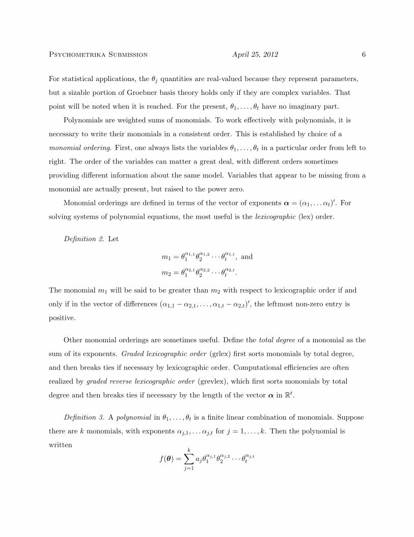
Polynomials are weighted sums of monomials. To work effectively with polynomials, it is
necessary to write their monomials in a consistent order. This is established by choice of a
monomial ordering. First, one always lists the variables θ1, . . . , θt in a particular order from left to
right. The order of the variables can matter a great deal, with different orders sometimes
providing different information about the same model. Variables that appear to be missing from a
monomial are actually present, but raised to the power zero.
Monomial orderings are defined in terms of the vector of exponents α = (α1, . . . αt)′. For
solving systems of polynomial equations, the most useful is the lexicographic (lex) order.
Definition 2. Let
m1 = θα1,1
1 θα1,2
2 · · · θα1,t
t , and
m2 = θα2,1
1 θα2,2
2 · · · θα2,t
t .
The monomial m1 will be said to be greater than m2 with respect to lexicographic order if and
only if in the vector of differences (α1,1 − α2,1, . . . , α1,t − α2,t)′, the leftmost non-zero entry is
positive.
Other monomial orderings are sometimes useful. Define the total degree of a monomial as the
sum of its exponents. Graded lexicographic order (grlex) first sorts monomials by total degree,
and then breaks ties if necessary by lexicographic order. Computational efficiencies are often
realized by graded reverse lexicographic order (grevlex), which first sorts monomials by total
degree and then breaks ties if necessary by the length of the vector α in Rt.
Definition 3. A polynomial in θ1, . . . , θt is a finite linear combination of monomials. Suppose
there are k monomials, with exponents αj,1, . . . αj,t for j = 1, . . . , k. Then the polynomial is
written
f(θ) =k∑j=1
ajθαj,1
1 θαj,2
2 · · · θαj,t
t
Psychometrika Submission April 25, 2012 7
The quantities being added are the terms of the polynomial. A term is a monomial multiplied by
a coefficient. The ordering of the terms in a polynomial corresponds to the order of the
monomials with respect to the chosen monomial ordering.
Definition 4. The leading term of a polynomial f = f(θ) is the one with the largest
monomial. It is denoted LT (f). The leading monomial is denoted LM(f), and the leading
coefficient is denoted LC(f). In terms of Definition 3,
LC(f) = a1
LM(f) = θα1,11 θα1,2
2 · · · θα1,t
t
LT (f) = a1θα1,11 θα1,2
2 · · · θα1,t
t
The coefficients a1, . . . , an are members of a field. A field is a set of objects, equipped with
operations corresponding to addition, subtraction, multiplication and division that satisfy the
usual rules. The set of real numbers is a field, as is the set of complex numbers. For moment
structure polynomials, the coefficients belong to a field that includes the moments σj ∈ R, so the
field of real numbers is a good choice for theoretical purposes. But for statistical applications, the
field of rational numbers may offer computational advantages.
Definition 5. Let F be a field. Then the set of all polynomials in θ1, . . . , θt with coefficients in
F is denoted F[θ1, . . . , θt].
So, R[θ1, . . . , θt] is the set of all polynomials in θ1, . . . , θt with real coefficients. Such a set
does not itself form a field, because only constant polynomials can have a multiplicative inverse.
They form a ring, specifically a commutative ring with unity. Groebner basis software, especially
of the non-commercial variety, may require the user to choose a polynomial ring.
Definition 6. Let F be a field and t be a positive integer. The t-dimensional affine space is
defined as
Ft = (x1, . . . , xt) : xj ∈ F for j = 1, . . . , t
The main examples are Rt and Ct.

Psychometrika Submission April 25, 2012 8
Ideal and Variety
Given a collection of polynomials in the variables (parameters) θ1, . . . , θt, the roots are the θ
values for which all the polynomials equal zero. If this set consists of just one point, all the
parameters are identifiable. The set of roots is called the variety.
Definition 7. The (affine) variety of a set of polynomials f1, . . . , fd ∈ F[θ1, . . . , θt] is the set of
points θ ∈ Ft where fj(θ) = 0 for j = 1, . . . , t.
Given a finite set of polynomials, it is clear that a much larger set of polynomials share the
same variety. In fact, if fj(θ) = 0, then the product of fj and any other polynomial will also equal
zero. This leads to an idea that is analogous to the concept of a vector space spanned by a set of
basis vectors, except that instead of being multiplied by constants, the basis polynomials are
multiplied by other polynomials.
Definition 8. Let f1, . . . , fd ∈ F [θ1, . . . , θt]. The ideal generated by the polynomials f1, . . . , fd
is defined by
〈f1, . . . , fd〉 = d∑i=1
hi(θ)fi(θ) : h1, . . . , hd ∈ F [θ1, . . . , θt]
The set 〈f1, . . . , fd〉 is closed under addition and multiplication, which is the definition of an
“ideal in a ring” from abstract algebra. The ideal generated by a collection of polynomials
represents all the polynomial consequences of setting the polynomials in the generating set to
zero. Some of these consequences may be simpler than any member of the generating set, because
multiplying polynomials and adding products can result in cancellations. For example, consider
the polynomials
f1 = θ31θ
22 + θ2
1θ32 − 2 θ2
1θ2 − 2 θ1θ22 + θ1 + θ2 (2)
f2 = −θ21θ2 − θ1θ
22 + 2 θ1 + θ2 − 1.
Using the well-chosen “weights” h1 = θ1 + θ2 and h2 = θ21θ2 + θ1θ
22 − θ2 − 1, the polynomial
combination g = h1f1 + h2f2 = θ21 − 2 θ1 + 1 = (θ1 − 1)2. The variable θ2 is eliminated from g, and

Psychometrika Submission April 25, 2012 9
substituting θ1 = 1 into f1 and f2 shows that the variety of f1, f2 consists of just two points:
(θ1 = 1, θ2 = 1) and (θ1 = 1, θ2 = −1). Thus, the ideal generated by a set of polynomials may
contain polynomials that are more helpful than any member of the generating set. In general, the
challenge is to find a set of nice, simple polynomials g1, . . . , gs ∈ 〈f1, . . . , fd〉 that have exactly the
same roots as f1, . . . , fd.
The polynomials f1, . . . , fd form a basis for the ideal they generate. Just as an ordinary
vector space has more than one possible basis, so does an ideal.
Definition 9. A set of polynomials p1, . . . , ps ∈ F [θ1, . . . , θt] is said to be a basis of an ideal I
if I = 〈p1, . . . , ps〉.
What makes it useful to seek another basis of the ideal generated by a set of polynomials is that if
two different sets of polynomials are bases of the same ideal, then they have the same roots. That
is, the solutions of the equations formed by setting all the polynomials to zero are the same for
the two sets.
Theorem 1. Let f = f1, . . . , fd and g = g1, . . . , gs be sets of polynomials in F [θ1, . . . , θt].
If 〈f1, . . . , fd〉 = 〈g1, . . . , gs〉, then the varieties of f and g are the same.
Groebner basis
For the two polynomials (2), the useful polynomial combination g = θ21 − 2θ1 + 1 ∈ 〈f1, f2〉 is
one of the polynomials of a Groebner basis for 〈f1, f2〉.
Definition 10. Given an ideal in I ⊂ F [θ1, . . . , θt], a Groebner basis for I is a finite set of
polynomials G = g1, . . . , gs ⊂ I such that for each polynomial f ∈ I, LT (f) = hLT (gi), for
some i ∈ 1, . . . , s, where h is a polynomial in F [θ1, . . . , θt].
Since ordinary long division may be applied to polynomials, one can say that the leading term of
each polynomial in the ideal is divisible by the leading term of some polynomial in the Groebner
basis. Note that which term of a polynomial is the leading term depends upon the monomial
Psychometrika Submission April 25, 2012 10
ordering, so one speaks a Groebner basis with respect to a particular monomial ordering. The
next theorem says that every non-zero ideal possesses a Groebner basis.
Theorem 2. For any non-zero ideal I ⊂ F [θ1, . . . , θt], there is a Groebner basis g1, . . . , gs
with gj ∈ I and 〈g1, . . . , gs〉 = I.
Long division
The existence of Groebner bases and some of their properties can be proved without ever
seeing one, but a systematic way of finding them depends upon long division of polynomials.
Long division of a polynomial by one other polynomial works just like ordinary long division,
yielding a unique quotient and remainder. There is also a standard algorithm (described by Cox
et al. among others, and implemented in many software packages) that divides a single
polynomial f by a set F = f1, . . . , fd, allowing f to be written
f(θ) = q1(θ)f1(θ) + · · ·+ qd(θ)fd(θ) + r(θ), (3)
where the polynomial qj is the quotient corresponding to fj for j = 1, . . . , d, and the polynomial r
is the remainder. The quotients and remainder are all elements of F [θ1, . . . , θt].
Unfortunately, this expression is not unique, and depends upon the ordering of f1, . . . , fd.
Worse, it is easy to divide f ∈ 〈f1, . . . , fd〉 by f1, . . . , fd and still obtain a remainder that is not
zero. However, the long division algorithm is more satisfactory when one is dividing by the
polynomials of a Groebner basis.
Theorem 3. Let G = g1, . . . , gs be a Groebner basis for the ideal I ⊂ F [θ1, . . . , θt], and let
the polynomial f ∈ F [θ1, . . . , θt]. Then the remainder upon division of f by G is unique, and does
not depend upon the ordering of g1, . . . , gs.
A Groebner basis for the ideal generated by a set of polynomials is obtained by iteratively
producing polynomials with simpler leading terms. This is accomplished using S-Polynomials (S
stands for subtraction), which can eliminate variables when the monomial ordering is
lexicographic, producing members of the ideal whose roots are potentially easier to find.
Psychometrika Submission April 25, 2012 11
Definition 11. Let m1 = θα11 · · · θαt
t and m2 = θβ11 · · · θβt
t be monomials. The least common
multiple of m1 and m2 is defined by LCM(m1,m2) = θγ11 · · · θγtt , where γi = max(αi, βi) for
i = 1, . . . , t.
Definition 12. Let the polynomials p, q ∈ F [θ1, . . . , θt]. The S-Polynomial is a combination of
p and q defined by
S(p, q) =`
LT (p)· p− `
LT (q)· q,
where ` = LCM (LM(p), LM(q)).
Again, LM(f) is the leading monomial of f .
To see how this works, adopt the lexicographic monomial ordering on the polynomials of (2),
with θ1 coming before θ2. The least common multiple of LM(f1) and LM(f2) is just the leading
monomial of f1, and the S-polynomial is
S(f1, f2) =θ31θ
22
θ31θ
22
· f1 −θ31θ
22
−θ21θ2
· f2 = f1 + θ1θ2f2 = −θ1θ22 − θ1θ2 + θ1 + θ2.
The S-polynomial is a member of 〈f1, f2〉 that is simpler than either of the generating
polynomials, and is a step in the right direction.
Even though S(f1, f2) is clearly a combination of the form (3) with quotients q1 = 1,
q2 = θ1θ2 and remainder r = 0, the long division algorithm cannot detect it, because it divides
S(f1, f2) by f1 and f2 one at a time. In either order, the remainder is just S(f1, f2). This cannot
happen when the input polynomials are part of a Groebner basis.
Theorem 4. Buchberger’s Criterion: Let I be a non-zero ideal of polynomials in F [θ1, . . . , θt].
Then a set of polynomials G = g1, . . . , gs is a Groebner basis for I if and only if for all pairs
i 6= j, the remainder upon division of S(gi, gj) by G equals zero.
Zero division upon remainder by a Groebner basis is a characteristic that the S-polynomials
share with all polynomials in the ideal.
Psychometrika Submission April 25, 2012 12
Theorem 5. Let I ⊂ F [θ1, . . . , θt] be an ideal, let G = g1, . . . , gs be a Groebner basis for I,
and let f ∈ F [θ1, . . . , θt]. Then f ∈ I if and only if the remainder upon division of f by G equals
zero.
Theorem 5 provides a general solution to the ideal membership problem. Given a set of
polynomials f1, . . . , fd and another polynomial f , how can one tell whether f is in the ideal
generated by f1, . . . , fd? That is, if f1(θ) = · · · = fd(θ) = 0, does it follow that f(θ) = 0? One
divides f by a Groebner basis for 〈f1, . . . , fd〉; the answer is yes if and only if the remainder is zero.
The missing ingredient is a systematic way of finding Groebner basis for the ideal generated
by a set of polynomials. The key is an iterative use of Buchberger’s Criterion. One computes
S-polynomials for all pairs of polynomials in the input set, dividing each S-polynomial by the
entire input set. If all remainders are zero, the set of polynomials is a Groebner basis by
Theorem 4, and the process terminates. Any remainder that is not zero is added to the input set,
and the process repeats. The following theorem says that this procedure converges in a finite
number of steps, yielding a set of polynomials that form a Groebner basis for 〈f1, . . . , fd〉.
Theorem 6. Buchberger’s Algorithm Let I = 〈f1, . . . , fd〉, where f1, . . . , fd ∈ F [θ1, . . . , θt]. A
Groebner basis G = g1, . . . , gs can be constructed in a finite number of steps by the algorithm
of Figure 1.
Reduction
Figure 1 portrays Buchberger’s original algorithm, which was designed more for proving
convergence than for computational efficiency. It can be and has been improved in various ways,
for example by not re-computing zero remainders; also see Tran (2000) and the references therein.
But all existing algorithms for computing Groebner bases work by adding polynomials to the
generating set, usually introducing some redundancy. In general Groebner bases are not unique,
and it is often possible to eliminate some of the polynomials and still have a Groebner basis for
the ideal in question.

Psychometrika Submission April 25, 2012 13
Figure 1.
Buchberger’s Algorithm: Input is a generating set of polynomials F = f1, . . . , fd. Output is a Groebner basis
G = g1, . . . , gs
.
Page 1 of 1
Consider a pair p,q, p≠q in G′
Compute the S-polynomial S(p,q)
Divide S(p,q) by G′. Remainder is r.
If r ≠ 0, let G = G ∪ r
Finished all (p,q) pairs?
G = G′?
Yes No
Finished. Groebner basis is G. Yes
No
Let G = F
Let G′ = G
Theorem 7. Let G = g1, . . . , gs be a Groebner basis for the ideal I ∈ F [θ1, . . . , θt]. If g ∈ G
is a polynomial whose leading monomial is a multiple of the leading monomial of some other
polynomial in G, then G ∩ gc is also a Groebner basis for I.
So by simply examining the leading terms, one can often locate redundant polynomials in a
Groebner basis and discard them. Usually, the polynomials that are discarded are earlier in the
list; the result is often that some or all of the original polynomials f1, . . . , fd disappear, and are
replaced by simpler ones.
Psychometrika Submission April 25, 2012 14
Reducing a Groebner basis happens in two steps. First, redundant members of the basis are
eliminated, and then the remaining ones are simplified one more time. The first step produces a
minimal Groebner basis, and the second step produces the reduced Groebner basis, which is
unique. These names are standard but unfortunate, because one would expect a “minimal”
quantity to simpler and more compact than a “reduced” one. But given a monomial order and an
ordering of variables, there are infinitely many minimal Groebner bases for a given ideal, each
with the same number of polynomials. One of these minimal bases is “reduced,” and is usually
the most informative.
Definition 13. A minimal Groebner basis for a non-zero polynomial ideal is a Groebner basis
G for I such that for every polynomial g ∈ G (a) The leading coefficient of g equals one, and (b)
The leading term of g is not a multiple of the leading term of any other polynomial in G.
Definition 14. A reduced Groebner basis for a non-zero polynomial ideal I is a Groebner
basis G for I such that for every polynomial g ∈ G, (a) The leading coefficient of g equals one,
and (b) No monomial of g is a multiple of the leading term of any other polynomial in G.
Theorem 8. Let G be a minimal Groebner basis for a non-zero polynomial ideal I. Replacing
each polynomial in G with its remainder upon division by the other polynomials in G yields a
reduced Groebner basis for I.
Theorem 9. A reduced Groebner basis is unique up to a monomial ordering and an ordering
of variables.
For the polynomials (2), the slightly improved Buchberger algorithm described by Cox et al.
in Section 2 of Chapter 9 yields the following Groebner basis with respect to lexicographic order.

Psychometrika Submission April 25, 2012 15
∼g1 = θ3
1θ22 + θ2
1θ32 − 2θ2
1θ2 − 2θ1θ22 + θ1 + θ2 (4)
∼g2 = −θ2
1θ2 − θ1θ22 + 2θ1 + θ2 − 1
∼g3 = −θ1θ2
2 − θ1θ2 + θ1 + θ2∼g4 = θ3
1 − 2θ21 + θ1θ2 − θ2 + 1
∼g5 = θ2
1 − 2θ1 + 1∼g6 = −θ1θ2 + θ3
2 − 2θ22 + 2
∼g7 = −θ1 + 2θ3
2 − 3θ22 − 2θ2 + 4
∼g8 = −2θ3
2 + 2θ22 + 2θ2 − 2
First, notice that∼g1= f1 and
∼g2= f2; the polynomials
∼g3, . . . ,
∼g8 have been added to the
original set to form a Groebner basis. Next, observe that the leading monomials of∼g1, . . . ,
∼g6 are
all multiples of LM(∼g7). So by Theorem 7, they may be discarded and the result is still a
Groebner basis for 〈f1, f2〉.
Dividing by leading coefficients yields a minimal Groebner basis.
−∼g7 = θ1 − 2θ3
2 + 3θ22 + 2θ2 − 4 (5)
−12
∼g8 = θ3
2 − θ22 − θ2 + 1
To convert this minimal Groebner basis to the reduced Groebner basis, each polynomial is
replaced by its remainder upon division by the other one. Dividing −∼g7 by −1
2
∼g8 yields
remainder θ1 + θ22 − 2, while dividing −1
2
∼g8 by −
∼g7 just returns the remainder −1
2
∼g8. Thus, by
Theorem 8, the reduced Groebner basis is
g1 = θ1 + θ22 − 2 (6)
g2 = θ32 − θ2
2 − θ2 + 1 = (θ2 + 1) (θ2 − 1)2 .
Psychometrika Submission April 25, 2012 16
The variable θ1 is eliminated from g2, and substituting the solutions for g2 = 0 into g1 shows
that the original polynomial equations f1 = f2 = 0 have exactly two real solutions: θ1 = 1, θ2 = 1
and θ1 = 1, θ2 = −1. This was not at all obvious from (2).
In this example, there are two polynomials in the original generating set and two polynomials
in the reduced Groebner basis, but that is a coincidence. There is no necessary relationship
between the number of generating polynomials and the number of polynomials in the reduced
Groebner basis.
Elimination
In the reduced Groebner basis (6), the second polynomial is a function of θ2 only, while the
first is a function of both θ1 and θ2. This is no accident. With the lexicographic monomial
ordering, the reduced Groebner basis is designed to eliminate variables one at a time in a manner
similar to the way Gaussian row reduction is used to solve systems of linear equations. The
elimination ideal formalizes the idea of eliminating variables. Let f1, . . . , fd be polynomials in
θ1, . . . , θt. The kth elimination ideal is the set of polynomial consequences of f1 = · · · = fd = 0
that do not involve θ1, . . . , θk, where k < t. That is, the first k variables are eliminated.
Definition 15. Let the polynomial ideal I = 〈f1, . . . , fd〉 ⊂ F [θ1, . . . , θt]. The kth elimination
ideal is defined by Ik = I ∩ F [θk+1, . . . , θt].
Theorem 10 is called the Elimination Theorem. It says that with the lexicographic monomial
ordering, the Groebner basis successively eliminates θ1, . . . , θt−1, provided such elimination is
possible.
Theorem 10. Let G be a Groebner basis for the non-zero polynomial ideal
I = 〈f1, . . . , fd〉 ⊂ F [θ1, . . . , θt] with respect to the lexicographic monomial ordering, with the
ordering of variables θ1, . . . , θt. For every 1 ≤ k ≤ t− 1, if the kth elimination ideal Ik 6= ∅, then
the set Gk = G ∩ F [θk+1, . . . , θt] 6= ∅, and Gk is a Groebner basis for Ik.
Let G = g1, . . . , gs be the reduced Groebner basis with respect to lexicographic order for
〈f1, . . . , fd〉, and list G in order of leading monomials, with the polynomial having the “largest”
Psychometrika Submission April 25, 2012 17
leading monomial coming first. If elimination of θ1, . . . , θt−1 from the system of equations is
possible, then gs (the last Groebner basis polynomial) will be a function of θt only. Suppose that
in addition, elimination of θ1, . . . , θt−2 is possible. Then gs−1 will be a function of θt−1 and
possibly θt, but not θ1, . . . , θt−2. The pattern continues, with only g1 being potentially a function
of all t parameters, again supposing that elimination is possible at each step. The result is a
system of polynomials in an upper triangular form similar to the row echelon form resulting from
Gaussian elimination in linear systems. As in the linear case, the solutions may be obtained by a
series of simple substitutions. By Theorem 1, these are also the solutions of the original system of
equations. Incidentally, calculation of the reduced Groebner basis for a set of polynomials that
are linear yields exactly the reduced row echelon form.
The ordering of variables θ1, . . . , θt has a profound effect upon the form of a Groebner basis
with respect to lexicographic order, because it determines which variables are eliminated. The
results of varying parameter order will be illustrated in the examples. Of course by Theorem 1,
the ordering of parameters ultimately has no effect upon the variety.
Sometimes, a variable cannot be eliminated, and two or more parameters appear for the first
time (reading from the bottom) in the same equation, possibly indicating that the system has
infinitely many solutions. This will be made precise in the next theorem.
Finiteness
Up to this point, all the definitions and theorems apply to an arbitrary field F , which could
be the set of real numbers. That is, the parameters θ1, . . . , θt may be real valued, as may the
coefficients in the set of polynomials F [θ1, . . . , θt]. But a rich and substantial portion of Groebner
basis theory applies only when the variables and coefficients are complex-valued, with potentially
both a real and an imaginary part. Many results in algebra are cleaner and more general as they
apply to complex numbers.
This account omits most parts of Groebner basis theory that require the parameters to be
complex variables. However, one result is useful in practice even though the parameters in most
statistical models are real-valued. Theorem 11 gives a necessary and sufficient condition for a
system of polynomial equations to have finitely many complex solutions. Since finitely many

Psychometrika Submission April 25, 2012 18
complex solutions implies finitely many real solutions, the theorem allows one to rule out
infinitely many real solutions for some models.
Theorem 11. Let V ⊂ Ct be the variety of the nonzero polynomial ideal I ⊂ C[θ1, . . . , θt], and
let G = g1, . . . , gs be a Groebner basis for I. Then V is a finite set if and only if for each j,
j = 1, . . . , t there is some mj ≥ 0 and some g ∈ G such that LM(g) = θmj .
That is, if each parameter θj appears to some non-zero power by itself as the leading
monomial of at least one Groebner basis polynomial, the system of polynomial equations has only
finitely many complex solutions. The case mj = 0 corresponds to a constant, non-zero
polynomial. Setting this polynomial to zero implies that the system has no solutions – and zero is
a finite number. This does not occur in structural modeling, because the system always has at
least one solution.
If any variable fails to appear by itself in a leading monomial, the system has infinitely many
complex solutions. There might be infinitely many real solutions, or there might be finitely many,
or only one. Further analysis is required.
For the example of the polynomials (2), a glance at either the raw Groebner basis (4), the
minimal basis (5) or the reduced basis (6) establishes that the system has finitely many complex
solutions and therefore finitely many real solutions.
Applications to structural modeling
Groebner basis methods clearly have the potential to reveal the identification status of
models to which standard rules do not apply. Less expected is their ability to yield statistics that
can be used to test model correctness, even for non-identifiable models.
Psychometrika Submission April 25, 2012 19
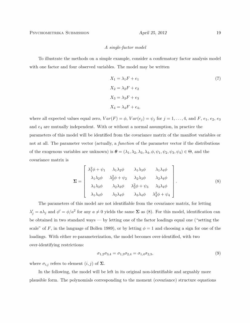
A single-factor model
To illustrate the methods on a simple example, consider a confirmatory factor analysis model
with one factor and four observed variables. The model may be written
X1 = λ1F + e1 (7)
X2 = λ2F + e2
X3 = λ3F + e3
X4 = λ4F + e4,
where all expected values equal zero, V ar(F ) = φ, V ar(ej) = ψj for j = 1, . . . , 4, and F , e1, e2, e3
and e4 are mutually independent. With or without a normal assumption, in practice the
parameters of this model will be identified from the covariance matrix of the manifest variables or
not at all. The parameter vector (actually, a function of the parameter vector if the distributions
of the exogenous variables are unknown) is θ = (λ1, λ2, λ3, λ4, φ, ψ1, ψ2, ψ3, ψ4) ∈ Θ, and the
covariance matrix is
Σ =
λ2
1φ+ ψ1 λ1λ2φ λ1λ3φ λ1λ4φ
λ1λ2φ λ22φ+ ψ2 λ2λ3φ λ2λ4φ
λ1λ3φ λ2λ3φ λ23φ+ ψ3 λ3λ4φ
λ1λ4φ λ2λ4φ λ3λ4φ λ24φ+ ψ4
. (8)
The parameters of this model are not identifiable from the covariance matrix, for letting
λ′j = aλj and φ′ = φ/a2 for any a 6= 0 yields the same Σ as (8). For this model, identification can
be obtained in two standard ways — by letting one of the factor loadings equal one (“setting the
scale” of F , in the language of Bollen 1989), or by letting φ = 1 and choosing a sign for one of the
loadings. With either re-parameterization, the model becomes over-identified, with two
over-identifying restrictions:
σ1,2σ3,4 = σ1,3σ2,4 = σ1,4σ2,3, (9)
where σi,j refers to element (i, j) of Σ.
In the following, the model will be left in its original non-identifiable and arguably more
plausible form. The polynomials corresponding to the moment (covariance) structure equations
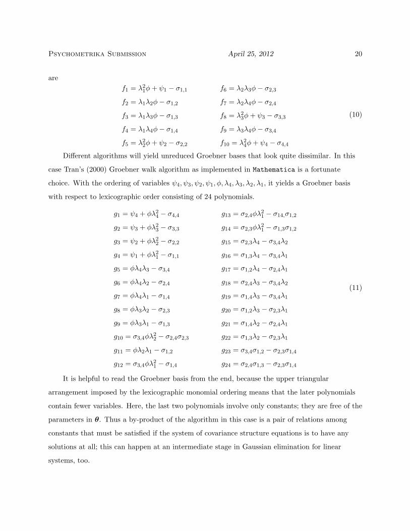
Psychometrika Submission April 25, 2012 20
aref1 = λ2
1φ+ ψ1 − σ1,1 f6 = λ2λ3φ− σ2,3
f2 = λ1λ2φ− σ1,2 f7 = λ2λ4φ− σ2,4
f3 = λ1λ3φ− σ1,3 f8 = λ23φ+ ψ3 − σ3,3
f4 = λ1λ4φ− σ1,4 f9 = λ3λ4φ− σ3,4
f5 = λ22φ+ ψ2 − σ2,2 f10 = λ2
4φ+ ψ4 − σ4,4
(10)
Different algorithms will yield unreduced Groebner bases that look quite dissimilar. In this
case Tran’s (2000) Groebner walk algorithm as implemented in Mathematica is a fortunate
choice. With the ordering of variables ψ4, ψ3, ψ2, ψ1, φ, λ4, λ3, λ2, λ1, it yields a Groebner basis
with respect to lexicographic order consisting of 24 polynomials.
g1 = ψ4 + φλ24 − σ4,4 g13 = σ2,4φλ
21 − σ14,σ1,2
g2 = ψ3 + φλ23 − σ3,3 g14 = σ2,3φλ
21 − σ1,3σ1,2
g3 = ψ2 + φλ22 − σ2,2 g15 = σ2,3λ4 − σ3,4λ2
g4 = ψ1 + φλ21 − σ1,1 g16 = σ1,3λ4 − σ3,4λ1
g5 = φλ4λ3 − σ3,4 g17 = σ1,2λ4 − σ2,4λ1
g6 = φλ4λ2 − σ2,4 g18 = σ2,4λ3 − σ3,4λ2
g7 = φλ4λ1 − σ1,4 g19 = σ1,4λ3 − σ3,4λ1
g8 = φλ3λ2 − σ2,3 g20 = σ1,2λ3 − σ2,3λ1
g9 = φλ3λ1 − σ1,3 g21 = σ1,4λ2 − σ2,4λ1
g10 = σ3,4φλ22 − σ2,4σ2,3 g22 = σ1,3λ2 − σ2,3λ1
g11 = φλ2λ1 − σ1,2 g23 = σ3,4σ1,2 − σ2,3σ1,4
g12 = σ3,4φλ21 − σ1,4 g24 = σ2,4σ1,3 − σ2,3σ1,4
(11)
It is helpful to read the Groebner basis from the end, because the upper triangular
arrangement imposed by the lexicographic monomial ordering means that the later polynomials
contain fewer variables. Here, the last two polynomials involve only constants; they are free of the
parameters in θ. Thus a by-product of the algorithm in this case is a pair of relations among
constants that must be satisfied if the system of covariance structure equations is to have any
solutions at all; this can happen at an intermediate stage in Gaussian elimination for linear
systems, too.

Psychometrika Submission April 25, 2012 21
Remarkably, setting the Groebner basis polynomials g23 and g24 to zero gives exactly the
over-identifying restrictions (9) that hold when this model is re-parameterized in either of the two
standard ways. Using the covariance matrix (8), it is easy to verify that these restrictions hold for
the non-identifiable version of the model as well. Thus, even a non-identifiable model can impose
testable equality constraints upon the moments, and these constraints may be revealed by a
Groebner basis. This suggests a general method for testing the correctness of models whose
parameters are not identifiable. Details are given in the Discussion section.
Polynomials g15 through g22 show the circumstances under which ratios of factor loadings are
identifiable. For example, setting g21 = g22 = 0, it is possible to solve for λ2λ1
at those points in the
parameter space where λ1 and at least two of λ2, λ3 and λ4 are not zero.
The set of polynomials g15 through g22 suggest the device of “setting the scale” of the factor
by letting one of the loadings equal unity (Bollen, 1989). For example, with λ1 = 1, the equations
corresponding to the Groebner basis polynomials are even easier to solve than (10). It is clear
from (11) that this is equivalent to a re-parameterization in which the factor loadings are
expressed in units of λ1, φ is expressed in units of 1λ21, and ψ1 through ψ4 are unchanged.
Groebner basis polynomials g12 through g14 reveal the circumstances under which another
function of the parameters is identifiable: φλ21. It is possible to solve for this quantity provided at
least one of σ2,3, σ2,4 and σ3,4 is non-zero, and hence that at least two of λ2, λ3 and λ4 are
non-zero.
Polynomials g12 through g14 suggest a second popular restriction commonly used to purchase
identification for confirmatory factor analysis models, namely setting φ = 1. Examination of g5
through g14 shows that if in addition the sign of one factor loading is known, this makes all the
factor loadings identifiable provided that at least three of them are not zero – a well known three
variable rule. It is also apparent from the Groebner basis that this is equivalent to a
re-parameterization in which the factor loadings are expressed in units of the standard deviation
of the underlying factor. All this is fairly obvious for a simple, familiar model like (7). What is
noteworthy is how easy it is to see from an unreduced Groebner basis.
The picture is much clearer for λ1 than for the other factor loadings even though by
symmetry, similar conclusions apply to all four loadings. The reason is that λ1 is listed last in the
Psychometrika Submission April 25, 2012 22
ordering of variables, so by the Elimination Theorem (Theorem 10), it plays a “starring role” in
the Groebner basis. With the lexicographic monomial ordering, conclusions appear most
explicitly for the variable listed last, with results for the other variables often appearing in terms
of the last variable.
Thus, it is often helpful to try more than one ordering of variables. In the present example,
listing ψ1, . . . , ψ4 last yields a Groebner basis with fifty (as opposed to 24) polynomials, twelve of
which show exactly where in the parameter space these four parameters are identifiable. This is a
bit more convenient than using g1, . . . , g4 in (11), but at the same time conclusions about
λ1, . . . , λ4 become less obvious. It is important to reiterate that all the possible Groebner bases
for a problem contain the same information in the sense that by Theorem 1, their polynomials
share a common set of roots. But different orderings of variables will cause this information to be
expressed differently, and can minimize the need for hand calculation.
So far, the unreduced Groebner bases for this factor analysis example have shown that
ψ1, . . . , ψ4 are identifiable almost everywhere in the parameter space, but have not yet revealed
lack of identifiability for the other parameters. In the Groebner basis (11), the failure of λ1 to
appear by itself in the leading term of any polynomial is a clue; by Theorem 11, this establishes
that the original set of polynomials (10) has infinitely many complex roots. But finitely many real
roots (or even a single real root) is still a mathematical possibility.
A firm conclusion comes from using Theorem 7 to discard polynomials whose leading terms
are multiples of other leading terms. To simplify the discussion, it will be assumed that all the
covariances are non-zero, limiting what follows to points where all the factor loadings are
non-zero; this applies to all but a set of volume zero in the parameter space. Working from the
bottom of the Groebner basis (11), the leading terms of g6, g10, g11 and g21 are all multiples of
LT (g22). Continuing in this fashion leaves g1, g2, g3, g4, g14, g17, g20 and g22, as well as g23 and g24.
Setting the last two polynomials to zero gives side conditions which must hold if the model is
correct, while the remaining Groebner basis polynomials correspond to eight equations in nine
unknowns. By the parameter count rule (see Appendix 5 of Fisher, 1966), these equations have
infinitely many real solutions, except possibly on a set of volume zero in R9, and hence in the
parameter space Θ. So, the vector of parameters (φ, λ1, λ2, λ3, λ4)′ is not identifiable, a conclusion
Psychometrika Submission April 25, 2012 23
that holds almost everywhere in the parameter space.
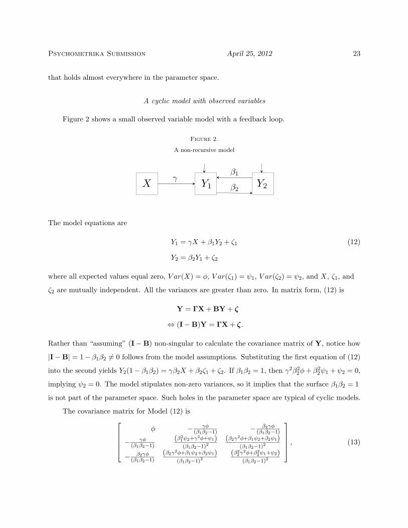
A cyclic model with observed variables
Figure 2 shows a small observed variable model with a feedback loop.
Figure 2.
A non-recursive model
X Y1 Y2!
!1
!2
The model equations are
Y1 = γX + β1Y2 + ζ1 (12)
Y2 = β2Y1 + ζ2
where all expected values equal zero, V ar(X) = φ, V ar(ζ1) = ψ1, V ar(ζ2) = ψ2, and X, ζ1, and
ζ2 are mutually independent. All the variances are greater than zero. In matrix form, (12) is
Y = ΓX + BY + ζ
⇔ (I−B)Y = ΓX + ζ.
Rather than “assuming” (I−B) non-singular to calculate the covariance matrix of Y, notice how
|I−B| = 1− β1β2 6= 0 follows from the model assumptions. Substituting the first equation of (12)
into the second yields Y2(1− β1β2) = γβ2X + β2ζ1 + ζ2. If β1β2 = 1, then γ2β22φ+ β2
2ψ1 + ψ2 = 0,
implying ψ2 = 0. The model stipulates non-zero variances, so it implies that the surface β1β2 = 1
is not part of the parameter space. Such holes in the parameter space are typical of cyclic models.
The covariance matrix for Model (12) isφ − γφ
(β1β2−1) − β2γφ(β1β2−1)
− γφ(β1β2−1)
(β21ψ2+γ2φ+ψ1)(β1β2−1)2
(β2γ2φ+β1ψ2+β2ψ1)(β1β2−1)2
− β2γφ(β1β2−1)
(β2γ2φ+β1ψ2+β2ψ1)(β1β2−1)2
(β22γ
2φ+β22ψ1+ψ2)
(β1β2−1)2
, (13)
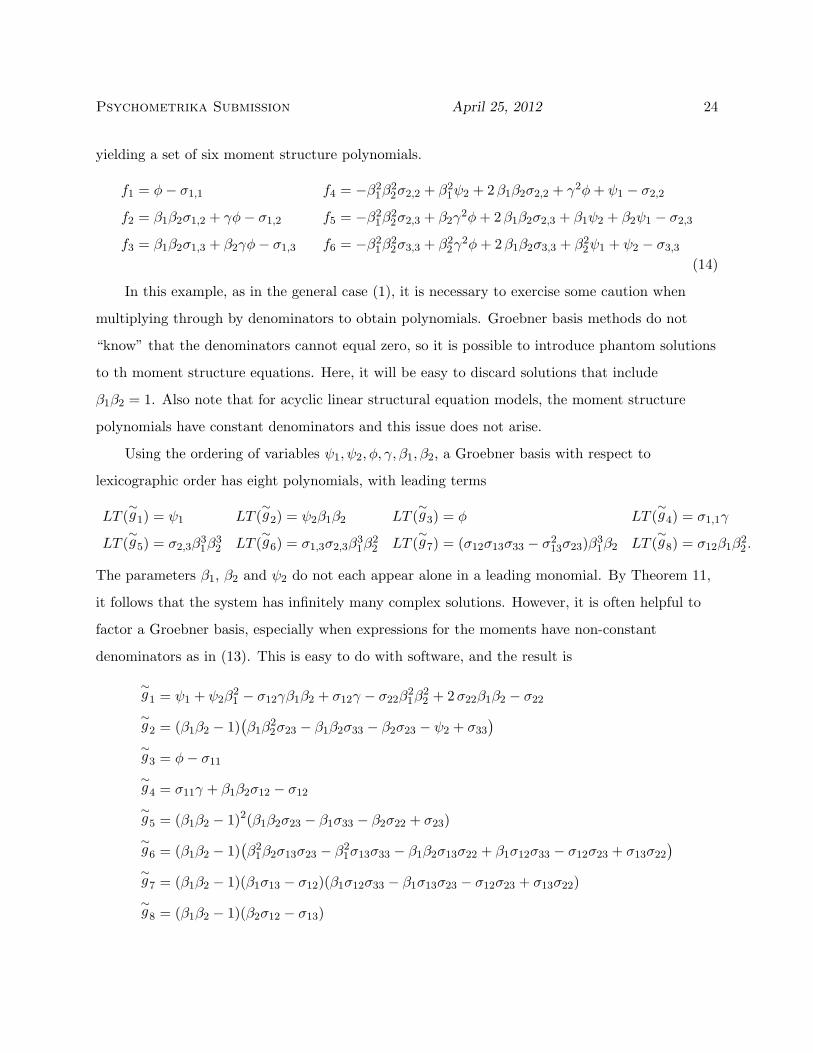
Psychometrika Submission April 25, 2012 24
yielding a set of six moment structure polynomials.
f1 = φ− σ1,1 f4 = −β21β
22σ2,2 + β2
1ψ2 + 2β1β2σ2,2 + γ2φ+ ψ1 − σ2,2
f2 = β1β2σ1,2 + γφ− σ1,2 f5 = −β21β
22σ2,3 + β2γ
2φ+ 2β1β2σ2,3 + β1ψ2 + β2ψ1 − σ2,3
f3 = β1β2σ1,3 + β2γφ− σ1,3 f6 = −β21β
22σ3,3 + β2
2γ2φ+ 2β1β2σ3,3 + β2
2ψ1 + ψ2 − σ3,3
(14)
In this example, as in the general case (1), it is necessary to exercise some caution when
multiplying through by denominators to obtain polynomials. Groebner basis methods do not
“know” that the denominators cannot equal zero, so it is possible to introduce phantom solutions
to th moment structure equations. Here, it will be easy to discard solutions that include
β1β2 = 1. Also note that for acyclic linear structural equation models, the moment structure
polynomials have constant denominators and this issue does not arise.
Using the ordering of variables ψ1, ψ2, φ, γ, β1, β2, a Groebner basis with respect to
lexicographic order has eight polynomials, with leading terms
LT (∼g1) = ψ1 LT (
∼g2) = ψ2β1β2 LT (
∼g3) = φ LT (
∼g4) = σ1,1γ
LT (∼g5) = σ2,3β
31β
32 LT (
∼g6) = σ1,3σ2,3β
31β
22 LT (
∼g7) = (σ12σ13σ33 − σ2
13σ23)β31β2 LT (
∼g8) = σ12β1β
22 .
The parameters β1, β2 and ψ2 do not each appear alone in a leading monomial. By Theorem 11,
it follows that the system has infinitely many complex solutions. However, it is often helpful to
factor a Groebner basis, especially when expressions for the moments have non-constant
denominators as in (13). This is easy to do with software, and the result is
∼g1 = ψ1 + ψ2β
21 − σ12γβ1β2 + σ12γ − σ22β
21β
22 + 2σ22β1β2 − σ22
∼g2 = (β1β2 − 1)
(β1β
22σ23 − β1β2σ33 − β2σ23 − ψ2 + σ33
)∼g3 = φ− σ11
∼g4 = σ11γ + β1β2σ12 − σ12
∼g5 = (β1β2 − 1)2(β1β2σ23 − β1σ33 − β2σ22 + σ23)∼g6 = (β1β2 − 1)
(β2
1β2σ13σ23 − β21σ13σ33 − β1β2σ13σ22 + β1σ12σ33 − σ12σ23 + σ13σ22
)∼g7 = (β1β2 − 1)(β1σ13 − σ12)(β1σ12σ33 − β1σ13σ23 − σ12σ23 + σ13σ22)∼g8 = (β1β2 − 1)(β2σ12 − σ13)
Psychometrika Submission April 25, 2012 25
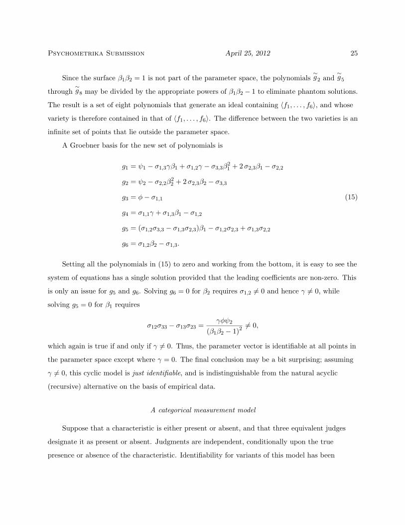
Since the surface β1β2 = 1 is not part of the parameter space, the polynomials∼g2 and
∼g5
through∼g8 may be divided by the appropriate powers of β1β2 − 1 to eliminate phantom solutions.
The result is a set of eight polynomials that generate an ideal containing 〈f1, . . . , f6〉, and whose
variety is therefore contained in that of 〈f1, . . . , f6〉. The difference between the two varieties is an
infinite set of points that lie outside the parameter space.
A Groebner basis for the new set of polynomials is
g1 = ψ1 − σ1,3γβ1 + σ1,2γ − σ3,3β21 + 2σ2,3β1 − σ2,2
g2 = ψ2 − σ2,2β22 + 2σ2,3β2 − σ3,3
g3 = φ− σ1,1 (15)
g4 = σ1,1γ + σ1,3β1 − σ1,2
g5 = (σ1,2σ3,3 − σ1,3σ2,3)β1 − σ1,2σ2,3 + σ1,3σ2,2
g6 = σ1,2β2 − σ1,3.
Setting all the polynomials in (15) to zero and working from the bottom, it is easy to see the
system of equations has a single solution provided that the leading coefficients are non-zero. This
is only an issue for g5 and g6. Solving g6 = 0 for β2 requires σ1,2 6= 0 and hence γ 6= 0, while
solving g5 = 0 for β1 requires
σ12σ33 − σ13σ23 =γφψ2
(β1β2 − 1)26= 0,
which again is true if and only if γ 6= 0. Thus, the parameter vector is identifiable at all points in
the parameter space except where γ = 0. The final conclusion may be a bit surprising; assuming
γ 6= 0, this cyclic model is just identifiable, and is indistinguishable from the natural acyclic
(recursive) alternative on the basis of empirical data.
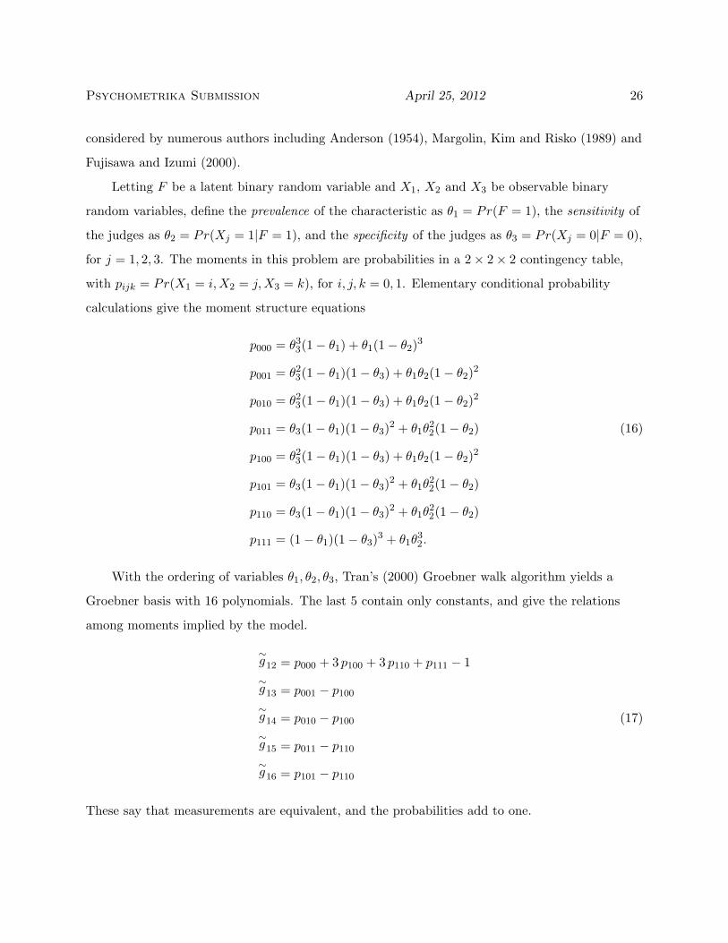
A categorical measurement model
Suppose that a characteristic is either present or absent, and that three equivalent judges
designate it as present or absent. Judgments are independent, conditionally upon the true
presence or absence of the characteristic. Identifiability for variants of this model has been
Psychometrika Submission April 25, 2012 26
considered by numerous authors including Anderson (1954), Margolin, Kim and Risko (1989) and
Fujisawa and Izumi (2000).
Letting F be a latent binary random variable and X1, X2 and X3 be observable binary
random variables, define the prevalence of the characteristic as θ1 = Pr(F = 1), the sensitivity of
the judges as θ2 = Pr(Xj = 1|F = 1), and the specificity of the judges as θ3 = Pr(Xj = 0|F = 0),
for j = 1, 2, 3. The moments in this problem are probabilities in a 2× 2× 2 contingency table,
with pijk = Pr(X1 = i,X2 = j,X3 = k), for i, j, k = 0, 1. Elementary conditional probability
calculations give the moment structure equations
p000 = θ33(1− θ1) + θ1(1− θ2)3
p001 = θ23(1− θ1)(1− θ3) + θ1θ2(1− θ2)2
p010 = θ23(1− θ1)(1− θ3) + θ1θ2(1− θ2)2
p011 = θ3(1− θ1)(1− θ3)2 + θ1θ22(1− θ2) (16)
p100 = θ23(1− θ1)(1− θ3) + θ1θ2(1− θ2)2
p101 = θ3(1− θ1)(1− θ3)2 + θ1θ22(1− θ2)
p110 = θ3(1− θ1)(1− θ3)2 + θ1θ22(1− θ2)
p111 = (1− θ1)(1− θ3)3 + θ1θ32.
With the ordering of variables θ1, θ2, θ3, Tran’s (2000) Groebner walk algorithm yields a
Groebner basis with 16 polynomials. The last 5 contain only constants, and give the relations
among moments implied by the model.
∼g12 = p000 + 3 p100 + 3 p110 + p111 − 1∼g13 = p001 − p100
∼g14 = p010 − p100 (17)∼g15 = p011 − p110
∼g16 = p101 − p110
These say that measurements are equivalent, and the probabilities add to one.
Psychometrika Submission April 25, 2012 27
The remaining 11 basis polynomials are very messy and uninformative, the longest having
102 terms; they will not be shown. Reducing the Groebner basis results in 15 polynomials rather
than 16, and all but the last five are long and difficult to look at. The polynomials do not factor,
and re-ordering the parameters makes no appreciable difference. This illustrates an unfortunate
reality that must be acknowledged. While a Groebner basis can yield valuable insight into some
problems, for others the result is simply unusable, usually because of the volume of output. Here,
the number of polynomials in the Groebner basis is modest, but they are long. In the final
example of this paper, the most natural way of expressing the problem results in a Groebner basis
with so many polynomials that the computation never finishes.
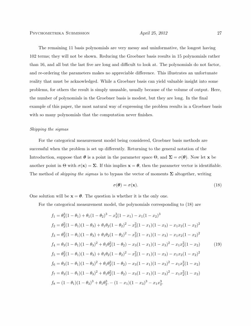
Skipping the sigmas
For the categorical measurement model being considered, Groebner basis methods are
successful when the problem is set up differently. Returning to the general notation of the
Introduction, suppose that θ is a point in the parameter space Θ, and Σ = σ(θ). Now let x be
another point in Θ with σ(x) = Σ. If this implies x = θ, then the parameter vector is identifiable.
The method of skipping the sigmas is to bypass the vector of moments Σ altogether, writing
σ(θ) = σ(x). (18)
One solution will be x = θ. The question is whether it is the only one.
For the categorical measurement model, the polynomials corresponding to (18) are
f1 = θ33(1− θ1) + θ1(1− θ2)3 − x3
3(1− x1)− x1(1− x2)3
f2 = θ23(1− θ1)(1− θ3) + θ1θ2(1− θ2)2 − x2
3(1− x1)(1− x3)− x1x2(1− x2)2
f3 = θ23(1− θ1)(1− θ3) + θ1θ2(1− θ2)2 − x2
3(1− x1)(1− x3)− x1x2(1− x2)2
f4 = θ3(1− θ1)(1− θ3)2 + θ1θ22(1− θ2)− x3(1− x1)(1− x3)2 − x1x
22(1− x2) (19)
f5 = θ23(1− θ1)(1− θ3) + θ1θ2(1− θ2)2 − x2
3(1− x1)(1− x3)− x1x2(1− x2)2
f6 = θ3(1− θ1)(1− θ3)2 + θ1θ22(1− θ2)− x3(1− x1)(1− x3)2 − x1x
22(1− x2)
f7 = θ3(1− θ1)(1− θ3)2 + θ1θ22(1− θ2)− x3(1− x1)(1− x3)2 − x1x
22(1− x2)
f8 = (1− θ1)(1− θ3)3 + θ1θ32.− (1− x1)(1− x3)3 − x1x
32.
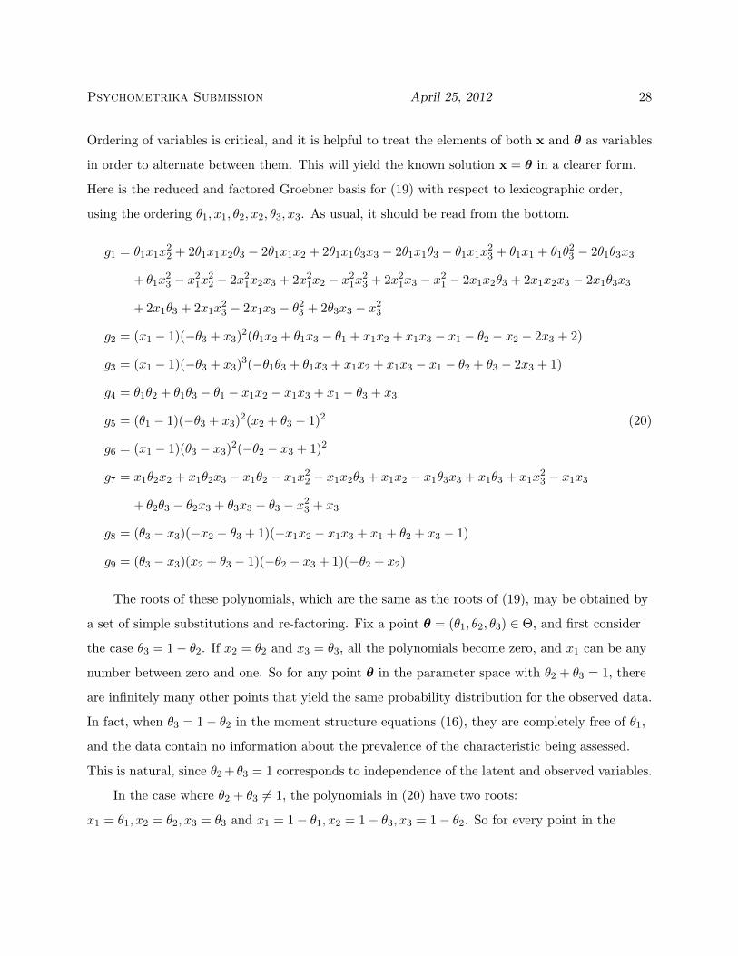
Psychometrika Submission April 25, 2012 28
Ordering of variables is critical, and it is helpful to treat the elements of both x and θ as variables
in order to alternate between them. This will yield the known solution x = θ in a clearer form.
Here is the reduced and factored Groebner basis for (19) with respect to lexicographic order,
using the ordering θ1, x1, θ2, x2, θ3, x3. As usual, it should be read from the bottom.
g1 = θ1x1x22 + 2θ1x1x2θ3 − 2θ1x1x2 + 2θ1x1θ3x3 − 2θ1x1θ3 − θ1x1x
23 + θ1x1 + θ1θ
23 − 2θ1θ3x3
+ θ1x23 − x2
1x22 − 2x2
1x2x3 + 2x21x2 − x2
1x23 + 2x2
1x3 − x21 − 2x1x2θ3 + 2x1x2x3 − 2x1θ3x3
+2x1θ3 + 2x1x23 − 2x1x3 − θ2
3 + 2θ3x3 − x23
g2 = (x1 − 1)(−θ3 + x3)2(θ1x2 + θ1x3 − θ1 + x1x2 + x1x3 − x1 − θ2 − x2 − 2x3 + 2)
g3 = (x1 − 1)(−θ3 + x3)3(−θ1θ3 + θ1x3 + x1x2 + x1x3 − x1 − θ2 + θ3 − 2x3 + 1)
g4 = θ1θ2 + θ1θ3 − θ1 − x1x2 − x1x3 + x1 − θ3 + x3
g5 = (θ1 − 1)(−θ3 + x3)2(x2 + θ3 − 1)2 (20)
g6 = (x1 − 1)(θ3 − x3)2(−θ2 − x3 + 1)2
g7 = x1θ2x2 + x1θ2x3 − x1θ2 − x1x22 − x1x2θ3 + x1x2 − x1θ3x3 + x1θ3 + x1x
23 − x1x3
+ θ2θ3 − θ2x3 + θ3x3 − θ3 − x23 + x3
g8 = (θ3 − x3)(−x2 − θ3 + 1)(−x1x2 − x1x3 + x1 + θ2 + x3 − 1)
g9 = (θ3 − x3)(x2 + θ3 − 1)(−θ2 − x3 + 1)(−θ2 + x2)
The roots of these polynomials, which are the same as the roots of (19), may be obtained by
a set of simple substitutions and re-factoring. Fix a point θ = (θ1, θ2, θ3) ∈ Θ, and first consider
the case θ3 = 1− θ2. If x2 = θ2 and x3 = θ3, all the polynomials become zero, and x1 can be any
number between zero and one. So for any point θ in the parameter space with θ2 + θ3 = 1, there
are infinitely many other points that yield the same probability distribution for the observed data.
In fact, when θ3 = 1− θ2 in the moment structure equations (16), they are completely free of θ1,
and the data contain no information about the prevalence of the characteristic being assessed.
This is natural, since θ2 + θ3 = 1 corresponds to independence of the latent and observed variables.
In the case where θ2 + θ3 6= 1, the polynomials in (20) have two roots:
x1 = θ1, x2 = θ2, x3 = θ3 and x1 = 1− θ1, x2 = 1− θ3, x3 = 1− θ2. So for every point in the
Psychometrika Submission April 25, 2012 29
parameter space where θ2 + θ3 6= 1, there is a point on the other side of the plane θ2 + θ3 = 1 that
yields the same set of probabilities for the observed data. Consequently, the likelihood function
will have exactly two maxima, one on either side of the plane. In practice, numerical search can
usually be limited to the set where θ2 + θ3 > 1, because as Zelen and Haitovsky (1991) observe,
θ2 + θ3 < 1 is equivalent to a negative association between manifest and latent variables.
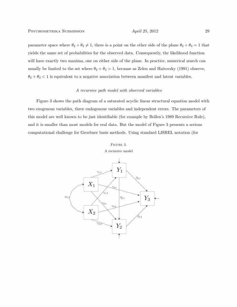
A recursive path model with observed variables
Figure 3 shows the path diagram of a saturated acyclic linear structural equation model with
two exogenous variables, three endogenous variables and independent errors. The parameters of
this model are well known to be just identifiable (for example by Bollen’s 1989 Recursive Rule),
and it is smaller than most models for real data. But the model of Figure 3 presents a serious
computational challenge for Groebner basis methods. Using standard LISREL notation (for
Figure 3.
A recursive model
X1
X2
Y2
Y1
Y3!1,2
!1,1
!2,1
!3,1
!1,2
!2,2
!3,2
!3,1
!2,1
!3,2

Psychometrika Submission April 25, 2012 30
example Joreskog, 1978), the moment structure polynomials may be written as
f1 = φ1,1 − σ1,1
...
f15 = β22,1β
23,2γ
21,1φ1,1 + 2β2
2,1β23,2γ1,1γ1,2φ1,2 + β2
2,1β23,2γ
21,2φ2,2 + 2β2,1β3,1β3,2γ
21,1φ1,1
+4β2,1β3,1β3,2γ1,1γ1,2φ1,2 + 2β2,1β3,1β3,2γ21,2φ2,2 + 2β2,1β
23,2γ1,1γ2,1φ1,1 + 2β2,1β
23,2γ1,1γ2,2φ1,2
+2β2,1β23,2γ1,2γ2,1φ1,2 + 2β2,1β
23,2γ1,2γ2,2φ2,2 + β2
2,1β23,2ψ1 + 2β2,1β3,2γ1,1γ3,1φ1,1
+2β2,1β3,2γ1,1γ3,2φ1,2 + 2β2,1β3,2γ1,2γ3,1φ1,2 + 2β2,1β3,2γ1,2γ3,2φ2,2 + β23,1γ
21,1φ1,1
+2β23,1γ1,1γ1,2φ1,2 + β2
3,1γ21,2φ2,2 + 2β3,1β3,2γ1,1γ2,1φ1,1 + 2β3,1β3,2γ1,1γ2,2φ1,2 + 2β3,1β3,2γ1,2γ2,1φ1,2
+2β3,1β3,2γ1,2γ2,2φ2,2 + β23,2γ
22,1φ1,1 + 2β2
3,2γ2,1γ2,2φ1,2 + 2β3,1β3,2γ1,2γ2,2φ2,2 + β23,2γ
22,1φ1,1
+2β23,2γ2,1γ2,2φ1,2 + β2
3,2γ22,2φ2,2 + 2β2,1β3,1β3,2ψ1 + 2β3,1γ1,1γ3,1φ1,1 + 2β3,1γ1,1γ3,2φ1,2
+2β3,1γ1,2γ3,1φ1,2 + 2β3,1γ1,2γ3,2φ2,2 + 2β3,2γ2,1γ3,1φ1,1 + 2β3,2γ2,1γ3,2φ1,2 + 2β3,2γ2,2γ3,1φ1,2
+2β3,2γ2,2γ3,2φ2,2 + β23,1ψ1 + β2
3,2ψ2 + γ23,1φ1,1 + 2 γ3,1γ3,2φ1,2 + γ2
3,2φ2,2 + ψ3 − σ5,5,
where the variances and covariances σi,j covariances are treated as constants.
When Groebner basis calculations are successful, they typically finish in a moment or two.
Here, using Sage version 4.3 and Mathematica versions 6.0, 7.0 and 8.0 on a variety of platforms
and operating systems, the calculation was stopped in each case after 24 hours. The algorithms
used were sophisticated versions, employing a variety of tricks to reduce the amount of
computation. A general idea of what happened can be obtained by tracing the behavior of a
slightly enhanced version of the Buchberger algorithm depicted in Figure 1; a convenient choice is
the Buch command in Gryc and Krauss’ Mathematica notebook for Mathematica 6
(http://www.cs.amherst.edu/∼dac/iva.html). The only modification of the original
Buchberger algorithm is that S-polynomials which have already been computed are not computed
again, and when a remainder is zero, the division of that S-polynomial by subsequent sets of
polynomials is skipped.
The first time through the main loop of Figure 1,(152
)= 105 S-polynomials are calculated,
and each is divided by the original set of 15 moment structure polynomials. Three remainders are
zero, so that 102 remainders are added to the set of polynomials. The next time through the loop,

Psychometrika Submission April 25, 2012 31
there are(1172
)= 6, 786 S-polynomials, of which 105 may be skipped. So 6, 786− 105 = 6, 681
divisions are performed. Only 200 remainders are zero, and the other 6,481 are added to the
input set of polynomials. There are now 15 + 102 + 6, 481 = 6, 598 polynomials, the longest with
441 terms. The third time through the loop, there are(6,598
2
)= 21, 763, 503 S-polynomials.
Skipping the ones that have already been computed, there are 21, 763, 503− 6, 786 = 21, 756, 717
remaining, each of which must be divided by the set of 6,598 polynomials. More than 24 hours of
computation are required, and in practice step 3 never finishes.
This example illustrates how rapidly the number of polynomials in an initial Groebner basis
can explode. The process is mathematically guaranteed to terminate eventually and reduction
along the way sometimes helps, but given current hardware and software, Groebner basis methods
sometimes just fail. While the initial number of polynomials is important, an even more critical
factor is the proportion of S-polynomials that have non-zero remainders. This, in turn, is
determined by the detailed structure of the polynomials and the way the problem is set up. For
example, when the method of “skipping the sigmas” (see Expression 18) is applied to the model
of Figure 3, computation is very fast and the Groebner basis consists of just 62 polynomials.
Once these are factored to locate and discard roots on the boundary of the parameter space,
identification follows immediately.
Discussion
For many structural statistical models, identifiability is determined by whether a system of
multivariate polynomial equations has more than one solution – or equivalently, whether a set of
multivariate polynomials has more than one simultaneous root. A Groebner basis for the ideal
generated by such a set of polynomials is another set of polynomials with the same set of
simultaneous roots, and those roots are often much easier to find starting with the Groebner
basis. For many models, a Groebner basis gives a clear picture of how identifiability changes in
different regions of the parameter space, and reveals functions of the parameters that are
identifiable even when the entire model is not.
Groebner basis theory reduces the process of simplifying multivariate polynomials to a
massive clerical task of the sort that is best handled by computer. Many symbolic mathematics
Psychometrika Submission April 25, 2012 32
programs have Groebner basis capability, and are very helpful for other modeling tasks such as
calculating covariance matrices, asymptotic standard errors and the like. Using the software is no
more difficult than using a statistics package, and familiarity with the material in this paper is
sufficient to allow informed application of the methods.
Problems that are resistant to elementary mathematics need present no particular difficulty.
For example, while the categorical measurement model discussed here is a familiar one that is
known to be identifiable with the appropriate restriction, the actual proofs of identifiably are
somewhat demanding (Anderson 1954; Teicher 1963). In contrast, a Groebner basis reveals the
same information for this model with minimal effort. The experience suggests that Groebner
basis methods may be helpful for studying global (rather than merely local) identifiability for less
tractable cases such as constrained categorical models with polytomous observed variables.
Testing fit of non-identifiable models
The factor analysis example shows how even a non-identifiable model can imply constraints
upon the moments, making it capable of being falsified by empirical data even though unique
estimation of its parameters is impossible. In this case and in many others, the constraints are
convenient by-products of Tran’s (2000) Groebner walk algorithm. But it is desirable to have a
method that is not tied to a particular algorithm, and to be certain that all the polynomial
relations among moments are represented, and that none of them is redundant. These goals may
be attained by considering the moments as variables rather than constants, and obtaining a
Groebner basis with respect to the lexicographic monomial ordering, making sure that the
moments appear after the parameters in the ordering of variables.
For a structural model with parameters θ1, . . . , θt and moments σ1, . . . , σd, suppose the
moment structure equations have the form f1 = · · · = fd = 0, where
f1, . . . , fd ∈ Q[θ1, . . . , θt, σ1, . . . , σd].
The notation Q indicates that the coefficients of the polynomials belong to the field of rational
numbers; in fact, they are usually integers.
The model-induced polynomial relations among σ1, . . . , σd are exactly the consequences of
Psychometrika Submission April 25, 2012 33
f1 = · · · = fd = 0 that do not involve θ1, . . . , θt. That is, they form an elimination ideal. Let
G = g1, . . . , gs be a Groebner basis for 〈f1, . . . , fd〉 with respect to lexicographic order. By
Theorem 10, the set of polynomials in G that are free of θ1, . . . , θt form a Groebner basis for the
elimination ideal 〈f1, . . . , fd〉 ∩Q[σ1, . . . , σd], and represent the equality constraints of the model.
For compactness and interpretability, it is desirable to express the Groebner basis for the
elimination ideal in reduced form. Carrying out the entire procedure for the factor analysis
example yields exactly (9), so that in this case the Groebner walk algorithm produces the desired
constraints in an optimal form even when the moments are treated as constants. The Groebner
walk algorithm does not always accomplish this for more complicated models, so it is preferable
to obtain the constraints by treating the moments as variables and calculating the reduced
Groebner basis for an elimination ideal.
The resulting constraints on the moments are the same as the null hypothesis that is tested
in a standard likelihood ratio test for goodness of model fit, provided that the maximum of the
likelihood function is in the interior of the parameter space. But Groebner basis methods yield
the constraints in an explicit form without the need to estimate model parameters. This means
models that are not identifiable may be confronted by data in a convenient way, without the need
to seek optimal constraints. When a non-identifiable model is consistent with the data, further
inference may be carried out entirely in the moment space. It is not necessary to assume a normal
distribution. For linear structural equation models, distribution-free versions of the tests may be
obtained using the Central Limit Theorem, assuming only the existence of fourth moments.
Drawbacks of Groebner basis methods
Groebner basis is not a panacea. One disadvantage comes from the very generality of the
theory. When using it to find the solutions of a set of moment structure equations, it is often
difficult to limit the answer to the parameter space. In the cyclic example and the categorical
example, it was possible to locate and discard solutions on the boundary of the parameter space
by factoring the Groebner basis. But for some models, even restricting solutions to the set of real
numbers can be a challenge.
Another disadvantage arises from the sheer volume of material that can be produced by
Psychometrika Submission April 25, 2012 34
Groebner basis software. While the polynomials in a Groebner basis are often simpler than those
the generating set, sometimes they are huge and ugly. This happened in the first try at the
categorical example. And because existing algorithms form an initial Groebner basis by adding
polynomials to the generating set, the number of polynomials can quickly become very large. As
a mathematical certainty, the algorithms will arrive at a Groebner basis in a finite number of
steps — but even with the fastest hardware currently available, there is no guarantee that this
will happen during one human lifetime. In the recursive path model example, the number of
polynomials exploded geometrically, and the computation never finished. This sort of difficulty is
well documented, and a great deal of effort has gone into methods for increasing the efficiency of
the computation. A special issue of the Journal of symbolic computation (Tran 2007) collects
recent developments as well as extensive references to the earlier literature.
For the recursive path model example as well as the categorical example, the Groebner basis
was unmanageable when the generating set of polynomials included symbols for the moments as
well as the parameters, but the “skipping the sigmas” setup of Expression 18 produced useable
results. This often happens, but skipping the sigmas discards information about model-induced
constraints on the moments. And for some larger problems, the computation still can take an
inordinately long time. For example, the industrialization and political democracy example
discussed by Bollen (1989, p. 333) features a three-variable recursive latent model and a
non-standard measurement model with several correlations between measurement errors. It has
eleven manifest variables and sixteen parameters. Groebner basis calculation for the entire model
never finishes even with skipping the sigmas, though it yields easily to a two-step approach in
which the latent variable model and the measurement model are analyzed separately. It is also
successful when the latent variable and measurement models are combined but the problem is
broken into parts by setting aside the diagonal elements of the covariance matrix.
The lesson is clear, if a little sobering. With current computer technology, simply encoding a
model with scores of parameters and throwing it at Groebner basis software is unlikely to succeed.
For such a model, one must resort to the same devices that would be helpful for doing the
problem by hand, such as breaking it into smaller pieces and reducing the number of variables by
making substitutions. Groebner basis will be most helpful with smaller parts of the problem that

Psychometrika Submission April 25, 2012 35
are unfamiliar or mathematically difficult.
One may confidently expect that as computer hardware continues to become faster and
algorithms continue to improve, Groebner basis methods will be applicable to larger and larger
problems. Even now, they can be a valuable tool for structural statistical modeling.
Psychometrika Submission April 25, 2012 36
References
Anderson, T.W. (1954). On estimation of parameters in latent structure analysis. Psychometrika
19(1), 1-10.
Bentler, P.M. & Weeks, D.G. (1980) Linear Structural Equations with Latent Variables,
Psychometrika, 45(3), 289-308.
Bezout, E. (2006). General theory of algebraic equations (Eric Feron, Trans.) Princeton, N.J.:
University Press. (Original work published 1779)
Bollen, K. A. (1989), Structural equations with latent variables, New York: Wiley.
Buchberger, B. (1965) Ein Algorithmus zum Auffinden der Basiselemente des Restklassenringes
nach einem Nulldimensionalen Polynomideal (An Algorithm for Finding the Basis Elements of
the Residue Class Ring of a Zero Dimensional Polynomial Ideal), Ph.D. Thesis, University of
Innsbruck. English translation by M. Abramson (2006) in Journal of Symbolic Computation
41, 471-511.
Cox, D., Little, J. and O’Shea, D. (2007). Ideals, Varieties, and Algorithms: An Introduction to
Computational Algebraic Geometry and Commutative Algebra, 3rd Edition, New York:
Springer-Verlang, Inc.
Decker, W., Greuel, G.-M., Pfister, G. & Schonemann, H. (2011). Singular 3-1-1 — A computer
algebra system for polynomial computations. http://www.singular.uni-kl.de.
Fisher, F. M. (1966) The Identification Problem in Econometrics, New York: McGraw-Hill.
Fujisawa, H. & Izumi, S. (2000). Inference about Misclassification Probabilities from Repeated
Binary Responses. Biometrics, 56(3), 706-711.
Garcıa-Puente, L. D., Spielvogel, S. and Sullivant, S. (2010). Identifying Causal Effects with
Computer Algebra, Proceedings of the 2010 Conference on Uncertainty in Artificial
Intelligence, Catalina Island, California, USA, July 8-11, 2010.
Grayson, D.R. & Stillman, M.E. (2011). Maccaulay2 — A software system for research in
algebraic geometry. http://www.math.uiuc.edu/Macaulay2/.

Psychometrika Submission April 25, 2012 37
Joreskog, K.G. (1978). Structural Analysis of Covariance and Correlation Matrices,
Psychometrika, 43(4), 443-477.
Koopmans, T.C. & Reiersøl, O. (1950). The Identification of structural characteristics. Annals of
Mathematical Statistics, 21(2), 165-181.
Margolin, B.H., Kim, B.S., & Risko, K.J. (1989). The Ames Salmonella/microsome mutagenicity
assay: Issues of inference and validation. Journal of the American Statistical Association 84,
651-661.
Maplesoft, Inc. (2008). Maple 12 user manual. Waterloo, Maplesoft.
McArdle, J.J. & McDonald, R. P. (1984). Some Algebraic Properties of the Reticular Action
Model, British Journal of Mathematical and Statistical Psychology, 37, 234-251.
McDonald, R.P. (1978). A Simple Comprehensive Model for the Analysis of Covariance
Structures, British Journal of Mathematical and Statistical Psychology, 31, 59-72.
Sitwell, J. (2010) Mathematics and its history, 3d Edition. New York: Springer.
Skrondal, A. & Rabe-Hesketh, S. (2004). Generalized latent variable modeling: Multilevel,
Longitudinal, and Structural Equation Models. New York: Chapman and Hall.
Stein, W.A. et al. (2010). Sage Mathematics Software (Version 4.2.1), The Sage Development
Team, http://www.sagemath.org.
Teicher, H. (1963). Identifiability of finite mixtures. Annals of Mathematical Statistics 34,
1265-1269.
Tran, Q.N. (2000). A fast algorithm for Grobner basis conversion and its applications. Journal of
Symbolic Computation, 30, 451-467.
Tran, Q. N. (2007). Special issue on applications of computer algebra. Journal of symbolic
computation, 42(5), 495-496.
Wall, M.M. & Amemiya, Y. (2000). Estimation for polynomial structural equations, Journal of
the American Statistical Association, 95(451), 929-940.
Psychometrika Submission April 25, 2012 38
Wall, M.M. & Amemiya, Y. (2003). A method of moments technique for fitting interaction effects
in structural equation models. British Journal of Mathematical and Statistical Psychology, 56,
4763.
Wolfram, S. (2003). The Mathematica Book (5th Edition), Champaign, Illinois: Wolfram Media,
Inc.
Zelen, M. and Haitovsky, Y. (1991). Testing hypotheses with binary data subject to
misclassification errors: Analysis and experimental design. Biometrika 78, 857-865.