The Groebner Factorizer and Polynomial System Solving

Talk given at the

Special Semester on Groebner Bases

Linz 2006

Hans-Gert GrabeDept. Computer Science, Univ. Leipzig, Germany

http://www.informatik.uni-leipzig.de/~graebe

February 28, 2006

1 Introduction

Let S := k[x1, . . . , xn] be the polynomial ring in the variables x1, . . . , xn over the field k andB := {f1, . . . , fm} ⊂ S be a finite system of polynomials. Denote by I(B) the ideal generated bythese polynomials. One of the major tasks of constructive commutative algebra is the derivationof information about the structure of

V (B) := {a ∈ Kn : ∀ f ∈ B such that f(a) = 0},

the set of common zeroes of the system B over an algebraically closed extension K of k.Splitting the system into smaller ones, solving them separately, and patching all solutions togetheris often a good guess for a quick solution of even highly nontrivial problems. This can be doneby several techniques, e.g., characteristic sets, resultants, the Groebner factorizer or some ad hocmethods. Of course, such a strategy makes sense only for problems that really will split, i.e., forreducible varieties of solutions. Surprisingly often, problems coming from “real life” fulfill thiscondition.

Among the methods to split polynomial systems into smaller pieces probably the Groebner factor-izer method attracted the most theoretical attention, see Czapor ([4, 5]), Davenport ([6]), Melenk,Moller and Neun ([16, 17]) and Grabe ([13, 14]). General purpose Computer Algebra Systems(CAS) are well suited for such an approach, since they make available both a (more or less) welltuned implementation of the classical Groebner algorithm and an effective multivariate polynomialfactorizer.Furthermore it turned out that the Groebner factorizer is not only a good heuristic approach forsplitting, but its output is also usually a collection of almost prime components. Their descriptionallows a much deeper understanding of the structure of the set of zeroes compared to the resultof a sole Groebner basis computation.Of course, for special purposes a general CAS as a multipurpose mathematical assistant can’t offerthe same power as specialized software with efficiently implemented and well adapted algorithmsand data types. For polynomial system solving, such specialized software has to implement twoalgorithmically complex tasks, solving and splitting, and until recently none of the specializedsystems (as e.g., GB, Macaulay, Singular, CoCoA, etc.) did both efficiently. Meanwhile, beingvery efficient computing (classical) Groebner bases, development efforts are also directed, not only

1

for performance reasons, towards a better inclusion of factorization into such specialized systems.Needless to remark that it needs some skill to force a special system to answer questions and theuser will probably first try his “home system” for an answer. Thus the polynomial systems solvingfacility of the different CAS should behave especially well on such polynomial systems that arehard enough not to be done by hand, but not really hard to require special efforts. It should invokea convenient interface to get the solutions in a form that is (correct and) well suited for furtheranalysis in the familiar environment of the given CAS as the personal mathematical assistant.

2 The Groebner Algorithm with Factorization

Define a zero set with constraints

V (B,C) := {a ∈ Kn : ∀ f ∈ B f(a) = 0 and ∀ g ∈ C g(a) 6= 0 },

This notion generalizes the notion of V (B).Note that C may be replaced for theoretical considerations by a single polynomial c =

∏g∈C g,

but the given notion has some advantage in handling constraints during computations.The Groebner algorithm with factorization (Groebner factorizer for short) addresses the following

General Problem

Given a system B = {f1, . . . , fm} ⊂ S of polynomials and a set of constraints C finda collection (Bα, Cα) of polynomial systems Bα in “triangular” form (for the moment:being a Groebner basis) and constraint sets Cα such that

V (B,C) =⋃α

V (Bα, Cα).

Using factorization this problem may be solved with the following algorithm

Factorized Groebner Bases FGB(B,C)

(1) During a preprocessing interreduce B and try to factor each polynomial f ∈ B. If f factors,replace B by a set of new problems, one for each factor of f . Update the side conditionsand apply the preprocessing recursively. This ends up with a list of interreduced problemswith non factoring base elements.

(2) For each basis in the problem list compute its list of critical pairs and put this Groebner taskinto the task list. Each Groebner task is a triple Tα = (Bα, Cα, Pα) where Bα is a partialGroebner basis and Pα the list of remaining pairs.

(3) Choose a Groebner task from the task list, run it in the usual way but try each reduced (nonzero) S-polynomial to factor before it will be added to the polynomial list. If it factors theninterrupt, split the task into as many subtasks as there are (different) factors, and put themback into the task list.

(4) If the Groebner task finished, extract the minimal Groebner basis of the subproblem.

If it is not yet reduced apply tail reduction to compute the minimal reduced Groebner basis.This may cause some of the base elements to factor anew. Apply the preprocessing oncemore.

If the result is stable then put it in the list of results.

Otherwise put the subproblems as new Groebner tasks back into the task list.

Obviously this algorithm terminates and returns a list of pairs (Bα, Cα) with the desired properties.The realization uses the following elementary operations :

2

1. Updating after factorization

If (B,C) is a problem and f ∈ I(B) factors as f = ga11 . . . gam

m then replace the problem bythe problem list

NewCon(B,C, {g1, . . . , gm}) := {(B ∪ {gi}, C ∪ {g1, . . . , gi−1}) | i = 1, . . . ,m}

2. Inconsistency check

(B,C) is inconsistent, i.e. V (B,C) = ∅, if the normal form NF (c,B) = 0 for some c ∈ C.

3. Subproblem removal check

(B1, C1) can be removed if there is a problem or partial result (B2, C2) such that V (B1, C1) ⊂V (B2). This occurs if NF (f,B1) = 0 for all f ∈ B2. The second problem has to be replacedby (B2, C1 ∩ C2).

Both checks use not the full power of information but only sufficient conditions. Indeed, the sidecondition C1 ∩C2 in (3) is weaker than the (logical) disjunction of C1 and C2. But the latter maynot correspond to a main open set in the Zariski topology. Since C1 ⊃ C and C2 ⊃ C we obtainnevertheless C1 ∩C2 ⊃ C. Hence the total set of solutions is not enlarged. This is the main pointto use constraint sets and not constraint polynomials.For (2), we remark that e.g. the full inconsistency check would need a radical membership test,i.e. another (full) Groebner basis calculation. This is impossible in the given frame since all checksmust be easy enough not to influence the performance of the main algorithm to heavily. If B is theGroebner basis of a prime ideal, NF (c,B) = 0 for some c ∈ C is also necessary for V (B,C) = ∅.Since our connection of factorization and Groebner basis computation leads often to such bases,one should force to progress with a subproblem as deep as possible to take best advantage of theside conditions (and the removal check).Splitting problems recursively in sets of subproblems yields a tree structure as described in [16]and conceptually used in both the REDUCE and the AXIOM implementations. Using a task listas in the approach described here has two advantages:

• It adds more flexibility in the choice (3) of the next Groebner task to be processed. Especially,splitting one of the leaves of the tree into subproblems one can queue up all these problemsand continue with a different subproblem. Compared to the recursive approach as e.g.implemented in AXIOM this may lead to a significant speedup, although by the abovetheoretical remark and empirical observations a depth first strategy has to be preferred.

• One can apply the subproblem removal check not only to the current task, but to all tasks(and results) queued up. This may lead to significant savings cancelling branches in an earlystage of the computation.

As explained above we should force a problem sort strategy that mimics a depth first recursionon the corresponding tree. We approximate this strategy sorting the problems by their virtualdimension. This is the dimension of the current Lt-ideal Lt(B). Computing new S-polynomialsthe Lt-ideal grows and hence its dimension may only decrease. Thus our strategy forces to treatGroebner tasks in greatest progress first.1.

3 The Preprocessing

We organized the preprocessing in a recursive way factoring each time a single basis element andthen interreducing and updating the corresponding subproblems before the preprocessor is called

1This is not the whole story since we use the easy linear time dimension algorithm, that works properly only forunmixed ideals, see [11]

3

on them anew. This has some advantage against the complete factorization of all base elementsin one step. To see this we restrict our considerations to ideals generated by monomials, this waydiscussing the influence of common factors occuring in several base elements on the preprocessing,but not the tail reduction effects derived from them.To compare our recursive approach with a complete factorization of all base elements, note thate.g. Reisner’s example, an ideal generated by 10 square-free monomials of degree 3, would splitinto 310 subproblems with the latter approach, whereas it splits into 10 prime monomial ideals with46 intermediate subproblems with the former one. This is true for almost all examples containingmany splitting basis elements. The following general example illustrates the situation once more :

Example:Im,n := I(x2k−1x2l : 1 ≤ k ≤ m, 1 ≤ l ≤ n)

As easily seen, Im,n = I(x2k−1 : 1 ≤ k ≤ m) ∩ I(x2l : 1 ≤ l ≤ n) decomposes finally into twosubproblems. Factoring all the mn generators at once and combining them to subsystems yields2mn different ideals (of coordinate hyperspaces). Two of them are the above minimal ones withrespect to inclusion.Using a recursive splitting argument we produce I(x2, x4, . . . , x2n) on the main branch and suc-cessively I0, I1, . . . , In−1 in the problem list with

I0 = I(x2m−1) + Im−1,n

andIk = I(x2m−1, x2n, . . . , x2(n−k)) + Im−1,n−k for k > 0.

Since I0 ⊂ . . . ⊂ In−1 only one problem survives and Im,n splits recursively generating only mnintermediate subproblems.

4 Solving polynomial systems – A short overview

Let’s first collect together some theoretical results and give a survey about the way solutions ofpolynomial systems may be represented. We only sketch the results below and refer the reader formore details to the papers [13, 14].Solving systems of polynomial equations in an ultimate way means to find a decomposition of thevariety of solutions into irreducible components, i.e., a representation of the radical Rad I(B) ofthe defining ideal as an intersection of prime ideals, and to present them in a way that is wellsuited for further computations. Usually one tries first to solve this problem over the ground fieldk, since the corresponding transformations may be performed without introducing new algebraicquantities. Only in a second step, K (or another extension of k) is involved. Since for generalunivariate polynomials of higher degree, there are no closed formulae for their zeroes using radicalsand moreover, even for equations of degree 3 and 4, the closed form causes great difficulties duringsubsequent simplifications, nowadays in most of the CAS the second step is by default not executed(in exact mode), but encapsulated in the functional symbol RootOf(p(x), x) 2, representing thesequence, set, list, etc. of solutions of the equation p(x) = 0 for a certain (in most cases notnecessarily irreducible) polynomial p(x). Hence we will not address the second step in the rest ofthis paper, too.Attempting to find a full prime decomposition leads to quite difficult computations (the approachdescribed in [9], and refined meanwhile in a series of papers, needs several Groebner basis compu-tations over different transcendental extensions of the ground field), involving generic coordinatechanges in the general case. The latter occurs, e.g., if one tries to separate the solution set of{x2 − 2, y2 − 2} over Q into the components {x2 − 2, y − x} and {x2 − 2, y + x}.

2We use this symbol to represent roots of univariate polynomials symbolically in a concise way, that is presentin similar versions, but under different names in almost all of the CAS under consideration.

4

Since the system {x2 − 2, y2 − 2} is already in a form convenient for computational purposes, onemay wish not to ask for a completely split, but for a triangular solution set. It turns out thatevery zero dimensional system of polynomials may be decomposed over k into such pieces evenwithout factorization.

4.1 Solving zero dimensional polynomial systems

The notion of triangular systems was introduced for zero dimensional ideals by Lazard in [15] andmeanwhile became widely accepted, see the monograph [18].A set of polynomials {f1(x1), f2(x1, x2), . . . , fn(x1, . . . , xn)} is a (zero dimensional) triangularsystem (reduced triangular set in [15]) if, for k = 1, . . . , n, fk(x1, . . . , xk) is monic (i.e., has aninvertible leading coefficient) regarded as a polynomial in xk over k[x1, . . . , xk−1], and the idealI = I(f1, . . . , fn) is radical, i.e., is an intersection of prime ideals. For such a triangular system, S/Iis a finite sum of algebraic field extensions of k. One can effectively compute in such extensions, aswas discussed in [15]. Lazard proposed to apply the D5 algorithm to decompose a zero dimensionalpolynomial system into triangular ones. There is also another approach, suggested in [19].

Proposition 1 ([15, 19]) Let B be a zero dimensional polynomial system.

1. If I(B) is prime then a lexicographic Groebner basis of B is triangular.

2. For an arbitrary B, there is an algorithm that computes a finite number of triangular systemsT1, . . . , Tm, such that

V (B) =⋃i

V (Ti)

is a decomposition (over k) of V (B) into pairwise disjoint sets of points.

Note that although such a decomposition may be found not involving any (full) factorizationbut only gcd computations, it is usually of great benefit to try to factor the system B first intosmaller pieces, since the size of the systems drastically influences the computation necessary for atriangulation.

4.2 Polynomial systems with infinitely many solutions

If P = I(B) is a prime ideal of positive dimension, the corresponding variety V (B) may beparameterized by the generic zero of P using reduction to dimension zero.For a given ideal I ⊂ S, and a subset V ⊂ {1, . . . , n}, the set of variables (xv, v ∈ V ) is anindependent set iff I ∩ k[xv, v ∈ V ] = (0). That is the variables (xv, v ∈ V ) are algebraicallyindependent mod I. Hence if (xv, v ∈ V ) is a maximal (with respect to inclusion) independent setfor the ideal I(B), these variables can be regarded as parameters whereas the remaining variablesdepend algebraically on them.This corresponds to a change of the base ring S −→ S := k(xv, v ∈ V )[xv, v 6∈ V ], where S isthe ring of polynomials in xv, v 6∈ V with coefficients in the function field k(xv, v ∈ V ). Thisbase ring extension corresponds to a localization at the multiplicative set of nonzero polynomialsin the variables (xv, v ∈ V ). The extension ideal I · S is a zero dimensional ideal in S and thealgorithms mentioned so far can be applied. For a prime ideal, we get I = I · S ∩ S, i.e., thegeneric zero describes a prime ideal I completely, presenting the quotient ring Q(S/I) = Q(S/I)as a finite algebraic extension of k(xv : v ∈ V ). For arbitrary ideals I(B), the localization maycut off some of the components of V (B) that must be parameterized separately. This can be donein an effective way, see [14].

As for zero dimensional ideals, such a presentation is not restricted to prime ideals. In moregenerality, let T = {f1, f2, . . . , fm} be a set of polynomials in S. We say that T forms a triangular

5

system with respect to the maximal independent set (xv, v ∈ V ) of I = I(T ) if the extension T ofT to S := k(xv, v ∈ V )[xv, v 6∈ V ] forms a triangular system for the (zero dimensional) extensionideal I := I · S.Such a triangular system may be regarded as a parameterization of V (IS ∩S), i.e., of the compo-nents of V (T ) missing the multiplicative set k[xv, v ∈ V ]\{0}. Hence a general polynomial systemsolver should (at least) decompose a given system of polynomials B into triangular systems, defin-ing for each of them the independent variables, extracting the part of V (B) parameterized thisway, and describing recursively the remaining part of V (B).

Altogether we can formulate the following

Polynomial System Solving Problem:

Given a finite set B ⊂ S of polynomials, find a collection (Tk, Vk) of triangular systemsTk with respect to Vk ⊂ {x1, . . . , xn}, such that

• Ik := I(Tk) · k(xv, v ∈ Vk)[xv, v 6∈ Vk]∩ S is a pure dimensional radical ideal withVk as a maximal strongly independent set,

• V (B) =⋃

V (Ik), and

• this decomposition is minimal.

Note that due to denominators occuring in k(xv, v ∈ Vk), the system Tk yields a parameterizationof only “almost all” points of V (Ik). By geometric reasons one cannot expect more, since evensimple examples of algebraic varieties show that a rational parameterization may miss some pointson the variety, see e.g., [3, chapter 3] for details. Since V (Ik) is the algebraic closure of theparameterized part, for each point X ∈ V (Ik), there is at least a curve of parameterized pointsapproaching X.

Let’s conclude this section with a little example:Consider the system B = {x3 − y2, x y − z}. A lexicographic Groebner basis computation yieldsG = {y5−z3, x z2−y4, x2 z−y3, x y−z, x3−y2}. Hence (z) is a maximal independent set by [11]and G′ = {y5 − z3, x (z2)− y4} a triangular system with respect to (z) (and a minimal Groebnerbasis of I(G) · S). Rewinding this tower of extensions over K, we get as parameterization of V (B)the five branches

{(z 25 , z

35 , z) : z ∈ K}

corresponding to the different choices of the branch of 5√

z. Note that these branches may beparameterized by a unique formula

V (B) = {(t2, t3, t5) : t ∈ K},

i.e., the variety is rational. It’s a deep geometric question to decide whether an irreducible varietyadmits a rational parameterization and in the case it does to find one, see e.g., [20]. Since none ofthe CAS under consideration invokes such algorithms with their solver, we will not address thisquestion here. Note that moreover in most applications, the structure of the prime components isvery easy. Often they may be either regularly (polynomially) parameterized (reg. par.)

{xk − pk(x1, . . . , xd) | k = d + 1, . . . , n}, pk ∈ k[x1, . . . , xd],

rationally parameterized (rat. par.)

{xk − pk(x1, . . . , xd) | k = d + 1, . . . , n}, pk ∈ k(x1, . . . , xd)

or are zero-dimensional primes in general position (g.p.)

{xk − pk(xn) | k = 1, . . . , n− 1} ∪ {pn(xn)}, pk ∈ k[xn].

6

5 A first example

To get a first impression about the power of the polynomial system solver implemented in differentCAS, let’s Solve a very simple one dimensional system like the Arnborg example A4, cf. [6].

vars := {w, x, y, z}polys := {wxy + wxz + wyz + xyz, wx + wz + xy + yz,

w + x + y + z, wxyz − 1}

The Groebner factorizer yields easily the following (already prime) decomposition into two onedimensional components:{

{w + y, x + z, yz − 1}, {w + y, x + z, yz + 1}}

Macsyma returns as answer the list

{{w = −%r5, x = 1%r5 , y = %r5, z = − 1

%r5},{w = −%r6, x = − 1

%r6 , y = %r6, z = 1%r6},

{w = −i, x = i, y = i, z = −i}, {w = i, x = −i, y = −i, z = i},{w = −1, x = 1, y = 1, z = −1}, {w = 1, x = −1, y = −1, z = 1},{w = −i, x = −i, y = i, z = i}, {w = i, x = i, y = −i, z = −i},{w = 1, x = 1, y = −1, z = −1}, {w = −1, x = −1, y = 1, z = 1}}

that contains the two expected one dimensional components together with a list of embeddedpoints.Mathematica returns the following result (slightly improved in 5.2)

{{w → − 1z , y → 1

z , x → −z}, {w → 1z , y → − 1

z , x → −z},{x → − 1

y , z → 1y , w → −y}, {x → 1

y , z → − 1y , w → −y}}

together with a warning

Solve::svars: Warning: Equations may not give solutionsfor all "solve" variables.

We obtain four instead of two solution sets, possibly according to the fact whether z 6= 0 or y 6= 0in y z − 1, respectively y z + 1. Such a distinction is unnecessary, since y z = 1 implies y, z 6= 0.MuPAD, Maple and Reduce return the solution in the expected form

{{x = −z, y = z−1, w = −z−1, z = z}, {x = −z, y = −z−1, w = z−1, z = z}}

Calling solve(polys,vars) with Axiom 2.0 ends up with the message

Error detected within library code:system does not have a finite number of solutions

whereas a direct call of the Groebner factorizer

groebnerFactorize polys

returns (almost) the expected answer

[[1], [z + x, y + w,wx + 1], [z + x, y + w,wx− 1]]

7

6 Solving zero dimensional systems

As explained above, zeroes of univariate polynomials of degree five don’t admit closed form rep-resentations in radicals in general and even for polynomials of degree 3 and 4, these expressionsare usually so difficult that they cause great trouble during simplification of derived expressions.Moreover the evident degree reduction rule for a single RootOf symbol leads to a normal repre-sentation of rational expressions containing this symbol. Hence it has become a certain standardto represent algebraic numbers even of small degree occuring in the solution set of a polynomialsystem through a RootOf construct.Functional symbols such as RootOf are ubiquitous objects in symbolic computations to constructnew symbolic expressions from old ones. The target of the simplification system of a CAS is tomake the inner world of the symbolic structure of the arguments cooperate with the outer worldof the environment of the functional symbol, e.g., expanding arguments over function symbols,collecting expressions together, or applying rules to combinations of symbols.In this context, the RootOf symbol plays a special role, since, different to most other functionalsymbols, it stands for a compound data structure and should expand in a proper way in differentsituations, i.e., expand partly or completely into the promised data structure under substitutionof values for parameters, during approximate evaluation, etc.The first three examples show how different CAS manage this difficulty.

Example 1:

vars := {x, y, z}polys := {x2 + y + z − 3, x + y2 + z − 3, x + y + z2 − 3}

This system has 8 different complex solutions. The set of solutions is stable under cyclic permuta-tions of the coordinates as are the equations. Note that the univariate polynomial of least degreein z (and, by symmetry, also in x and in y) belonging to I(polys) has only degree 6.Systems that involve factorization have no trouble decomposing this system. The CAS underconsideration answer in the following way:

Maple:

sol := {{y = −3, x = −3, z = −3}, {z = 1, x = 1, y = 1},

{z = RootOf( Z 2 − 2), y = RootOf( Z 2 − 2),x = −RootOf( Z 2 − 2) + 1},

{z = RootOf( Z 2 − 2), y = −RootOf( Z 2 − 2) + 1,x = RootOf( Z 2 − 2)},

{x = −RootOf(−2 Z − 1 + Z 2) + 1, z = RootOf(−2 Z − 1 + Z 2),y = −RootOf(−2 Z − 1 + Z 2) + 1}}

Axiom:sol := [[x = 1, y = 1, z = 1], [x = −3, y = −3, z = −3],

[x = −z + 1, y = −z + 1, 2z2 − 2z − 1 = 0],[x = z, y = −z + 1, z2 − 2 = 0], [x = −z + 1, y = z, z2 − 2 = 0]]

Macsyma and Reduce:

sol := {{x =√

2 + 1, y = −√

2, z = −√

2}, {x =√

2, y =√

2, z = −√

2 + 1},{x =

√2, y = −

√2 + 1, z =

√2}, {x = −

√2 + 1, y =

√2, z =

√2},

{x = −√

2, y =√

2 + 1, z = −√

2}, {x = −√

2, y = −√

2, z =√

2 + 1},{x = 1, y = 1, z = 1}, {x = −3, y = −3, z = −3}}

8

Mathematica and MuPAD have some trouble to extract the solution set in such clarity but leavenested roots. {

[x = 1, y = 1, z = 1] ,

[x = −3, y = −3, z = −3] ,[x =

√2, y =

√2, z = 1−

√2],[

x = −√

2, y = −√

2, z =√

2 + 1],[

x =

√4√

2 + 92

+ 1/2, y = 1/2−√

4√

2 + 92

, z = −√

2

],[

x =

√9− 4

√2

2+ 1/2, y = 1/2−

√9− 4

√2

2, z =

√2

],[

x = 1/2−√

4√

2 + 92

, y =

√4√

2 + 92

+ 1/2, z = −√

2

],[

x = 1/2−√

9− 4√

22

, y =

√9− 4

√2

2+ 1/2, z =

√2

] }We conclude, that (for multivariate systems) Maple and Axiom use the RootOf notation even foralgebraic numbers of degree 2 whereas Reduce, Macsyma and Mathematica promise to handlesuch square root symbols as “normal” numbers. But even simple square roots of integers mayalready cause trouble as in the Mathematica output of the solution above. Although Reduce hasno problem handling the square roots here, in general it often runs into trouble with the defaultsetting of the switch rationalize to off. Correct (in the given context) simplifications of squareroots of complicated symbolic expressions cause problems to all the CAS under consideration, seee.g., example 10 below.Note that although Maple offers quite powerful algorithms to deal with the RootOf symbol, thereturn data type design of RootOf(P (x), x) is not satisfactory. Due to the above syntax, it promisesto return one of the roots of P (x) instead all of them. Hence different calls to RootOf should choosesuch a root independently. This is required for different elements of sol, but not for different callsof RootOf inside the same element of sol. The procedure allvalues tries to expand the differentroots properly either in radicals (up to degree 4) or to approximate them numerically. It may becalled with a second parameter d to indicate that the same RootOf symbol in different places hasto be expanded identically3. Issuing

map(allvalues,sol,d);

we obtain the same answer as Macsyma and Reduce for this example. Note that this approachruns into trouble with nested RootOf expressions in example 4 below.The concisest solution for these problems is offered by Mathematica: It’s Roots command returns a(promise of a) logical conjunction of zeroes that is handled properly by subsequent substitutions,approximate evaluations, etc. The ToRules operator transforms such a logical expression intoa Sequence, i.e., (a promise of) comma separated expressions that automatically expand in theargument list of functional symbols with variable argument list length (Set, List, etc.) wheneverpossible. For example, the parametric equation f = x5 − 5x3 + 4x + a yields with

Solve[f==0,x]

3d was changed to dependent in Maple version V.4.

9

the answer{ToRules[Roots[4x− 5 x3 + x5 = −a, x]]}

that expands under the substitution %/.a → 0 automatically into

{{x → 2}, {x → 1}, {x → 0}, {x → −1}, {x → −2}}

Reduce uses the RootOf symbol in a sense like Maple, but binds its value for a single solution toa variable, hence resolving the ambiguity discussed above in a proper way. Expansion into a listof individual solutions is done in two steps. First, the RootOf symbol is changed automaticallyinto the one of symbol with the desired list as argument. Second, the user may call the commandexpand cases to expand this functional expression properly inside a list of solutions. For thepolynomial f , we get successively

solve(f,x);

{x = root of(a + x5 − 5 · x3 + 4 · x, x)}

sub(a=0,ws);

{x = one of({2, 1, 0, −1, −2})}

expand cases(ws);

{x = 2, x = 1, x = 0, x = −1, x = −2}.

Axiom follows another strategy. It doesn’t introduce RootOf symbols in the output of the solvecommand, but returns a list of (simplified) systems of equations instead, that may be furthersimplified with the usual system command. To extract, e.g., (real) approximate solutions fromthe above symbolic answer one may call

realsol:=concat([solve(u,0.001) for u in sol])

and then check the answer by

[[subst(u,v) for u in polys] for v in realsol].

A great difficulty for the CAS that use a RootOf notion remains the proper simplification ofexpressions involving such symbols. A good benchmark for these capabilities is the resubstitutiontest, i.e., the test whether the CAS may prove that the produced solutions satisfy the initialequations. In our experiments, only Maple was able to do these simplifications with satisfactorysuccess, possibly after a subsequent call to the algebraic simplifier evala, that is not invoked withsimplify.

Example 2:

vars := {x, y}polys := {x4 + y + 1, y4 + y + 1}

This example has 16 different complex solutions, none of them being real. It demonstrates boththe difference between an early use of RootOf expressions as in Axiom, Maple and Reduce, full

10

radical expansion of solutions of equations up to degree 4 as in Mathematica, and the differencebetween triangular systems and a complete decomposition into isolated prime components4.To begin with, note that for x > y, the given system of equations is already in triangular form.Moreover, it is easily seen that x4−y4 belongs to I(polys), i.e., the solution set may be decomposedinto

V (polys) = V (x + y, y4 + y + 1) ∪ V (x− y, y4 + y + 1) ∪ V (x2 + y2, y4 + y + 1).

Reduce ends up with the original triangular systems

sol := {{x = RootOf(x4 + x + 1, x), y = RootOf(x + y4 + 1, y)}}

whereas Maple and Axiom find the decomposition (probably by some ad hoc method).Mathematica computes 16 explicit solutions sol, very complicated formulae, that it isn’t able tohandle further symbolically. For example, the test

polys/.sol//Simplify

fails to return 0. Checking the numerical approximations N[sol] with

polys/.N[sol]

we detect 8 of the 16 approximations to be wrong.5

Macsyma resolves all that “trouble” in a different way: If results become too complicated itswitches automatically to numerical solutions. For this purpose there are several root finding de-vices as e.g., for real and complex roots, for counting roots inside a real interval, for approximationof roots by different methods, etc. No RootOf philosophy is supported. Of course, such an ap-proach doesn’t work for equations with parametric coefficients as e.g., for f = x5−5x3+4x+a. Forthose systems, Macsyma follows the same philosophy as Axiom, i.e., returns simplified equationsthat may be subsequently handled with the Lisp-like system language.

Let’s digress for a moment to the numerical solving capabilities for zero dimensional systems offeredby the other CAS in the case the user isn’t satisfied with the symbolic answer (as it probably willbe the case in our situation).As we already mentioned, Mathematica is best suited for such approximate solutions, since thenumerical evaluator may be involved in a unified way in almost all situations. Besides the easy(but in this case wrong) approximate evaluation of the symbolic results themselves, one can alsosolve the system approximately with

NSolve[polys,vars]

to obtain 16 correct solutions.For Axiom we may proceed as above. Starting from the symbolic solution

sol:=solve(polys,vars)

the complex system’s solver

csol:=concat([complexSolve(u,0.00001) for u in sol])

4MuPAD returns the strange answer{[y = RootOf(−y2 + RootOf(x + y2 + 1, y)), x = RootOf(x + x4 + 1)]}.

5Note that this default behaviour may be turned off bySetOptions[Roots,Cubics-¿False,Quartics-¿False]

Then the resulting expression is evaluated numerically in a proper way.

11

may be involved. It returns 16 complex solutions that may be checked to be correct in the samemanner as above

[[subst(u,v) for u in polys] for v in csol]

Reduce invokes approximate algorithms, switching with on rounded to floating point arithmetic.Calling solve(polys,vars) directly returns the 16 complex solutions. The situation becomesmore difficult starting from the symbolic solution sol. Switching to floating point arithmetic, theroot of expressions are changed into one of expressions

{{x = one of({0.934099289461 ∗ i + 0.727136084491, . . .}),y = one of({(−(x + 1))0.25 ∗ i, . . .})}},

that may be expanded via Expand Cases into 16 complex solutions

{{x = 0.934099289461 ∗ i + 0.727136084491, y = (−(x + 1))0.25 ∗ i}, . . .}

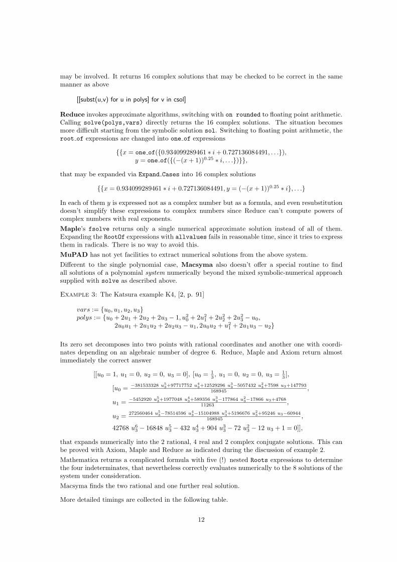
In each of them y is expressed not as a complex number but as a formula, and even resubstitutiondoesn’t simplify these expressions to complex numbers since Reduce can’t compute powers ofcomplex numbers with real exponents.Maple’s fsolve returns only a single numerical approximate solution instead of all of them.Expanding the RootOf expressions with allvalues fails in reasonable time, since it tries to expressthem in radicals. There is no way to avoid this.MuPAD has not yet facilities to extract numerical solutions from the above system.Different to the single polynomial case, Macsyma also doesn’t offer a special routine to findall solutions of a polynomial system numerically beyond the mixed symbolic-numerical approachsupplied with solve as described above.

Example 3: The Katsura example K4, [2, p. 91]

vars := {u0, u1, u2, u3}polys := {u0 + 2u1 + 2u2 + 2u3 − 1, u2

0 + 2u21 + 2u2

2 + 2u23 − u0,

2u0u1 + 2u1u2 + 2u2u3 − u1, 2u0u2 + u21 + 2u1u3 − u2}

Its zero set decomposes into two points with rational coordinates and another one with coordi-nates depending on an algebraic number of degree 6. Reduce, Maple and Axiom return almostimmediately the correct answer

[[u0 = 1, u1 = 0, u2 = 0, u3 = 0], [u0 = 13 , u1 = 0, u2 = 0, u3 = 1

3 ],

[u0 = −381533328 u53+97717752 u4

3+12529296 u33−5057432 u2

3+7598 u3+147793168945 ,

u1 = −5452920 u53+1977048 u4

3+589356 u33−177864 u2

3−17866 u3+476811263 ,

u2 = 272560464 u53−78514596 u4

3−15104988 u33+5196676 u2

3+95246 u3−60944168945 ,

42768 u63 − 16848 u5

3 − 432 u43 + 904 u3

3 − 72 u23 − 12 u3 + 1 = 0]],

that expands numerically into the 2 rational, 4 real and 2 complex conjugate solutions. This canbe proved with Axiom, Maple and Reduce as indicated during the discussion of example 2.Mathematica returns a complicated formula with five (!) nested Roots expressions to determinethe four indeterminates, that nevertheless correctly evaluates numerically to the 8 solutions of thesystem under consideration.Macsyma finds the two rational and one further real solution.

More detailed timings are collected in the following table.

12

symbSolve numSolve1 numSolve2time structure time structure time structure

Axiom 10.8 (2x1 1x6) 134.6 8 sol. 176.2 8 sol.Macsyma 10.2 3 sol. — —Maple 1.6 (2x1 1x6) — 0.3 8 sol.Mathem. 0.4 5 nested Roots 0.5 6 sol. 0.1 8 sol.Reduce 0.6 (2x1 1x6) 2.6 8 sol. 0.5 8 sol.

Table 1 a: Solving example 3

The first two columns (symbSolve) are devoted to the symbolic solver’s behaviour. The structurecolumn collects information about the degrees of the different branches. The latter columnsdescribe the numeric solver’s output (numSolve1) and the numeric approximation of the symbolicresults (numSolve2) as far as they may be computed. All timings are given in seconds of CPU-timeas reported by the corresponding CAS.

Let’s conclude this section with some more difficult examples, collecting the results in Tables 1 b– 1 e.

Example 4:

vars := {x, y, z}polys := {x3 + y + z − 3, x + y3 + z − 3, x + y + z3 − 3}

The result contains several branches of degree 6, some of them are quadratic extensions of cubicones. This explains the different branching of Reduce compared to Maple and Axiom.

symbSolve numSolve1 numSolve2time structure time structure time structure

Axiom 61.9 (1x1 1x2 4x6) 383 27 sol. 251 27 sol.Macsyma 39.9 25 sol. — —Maple 2.8 (1x1 1x2 4x6) — 1.8 39 sol.Mathem. 160.7 11 branches 0.54 18 sol. 0.4 21 sol.Reduce 1.7 (3x1 2x3 3x6) 14.4 27 sol. 1.5 27 sol.

Table 1 b: Solving example 4

Note that both Maple and Mathematica expand their symbolic results into a wrong number ofsolutions. Maple expands one of the branches of degree 6 improperly: A RootOf symbol of degree 2nested with another RootOf symbol of degree 3 is expanded into 18 instead of 6 solutions, probablydue to a wrong application of allvalues. Surprisingly enough, resubstitution proves only 6 ofthese solutions to be wrong.

Example 5: The Arnborg example A5, [6], also known as “cyclic 5”

vars := {v, w, x, y, z}polys := {v + w + x + y + z, v w + v z + w x + x y + y z,

v w x + v w z + v y z + w x y + x y z,v w x y + v w x z + v w y z + v x y z + w x y z, v w x y z − 1}

This is already a quite hard example. The ideal is radical and of degree 70, i.e., has 70 differentcomplex solutions.

13

symbSolve numSolve1 numSolve2time structure time structure time structure

Axiom 34 677 (5x2 15x4) 49 276 70 sol. 202 70 sol.Maple 740 (5x2 10x4 2x16) — zero divide error

Reduce 13.5 (10x1 12x4 1x12) 82.4 70 sol.RootOf not prop-erly expanded

Table 1 c: Solving example 5

Macsyma and Mathematica were unable to crack this example. MuPAD returned a strange result,consisting of a single branch containing an equation of degree 15 for z and an equation of degree 2depending on z for y. Altogether this may be expanded into at most 30 solutions. For numSolve2,Reduce couldn’t resolve the complicated RootOf expression properly. Maple couldn’t expand thesymbolic branches, too, but crashed with a zero divide error.

Example 6:

vars := {x, y, z}polys := {x3 + y2 + z − 3, x + y3 + z2 − 3, x2 + y + z3 − 3}

This is a slightly more complicated example than example 1 or example 4 from a series of systemsthat are symmetric under cyclic permutations.

symbSolve numSolve1 numSolve2time structure time structure time structure

Axiom 47.7 (1x1 1x2 1x24) > 25 000 > 25 000Macsyma 36.7 25 sol. — —Maple 11.3 (1x1 1x2 1x24) — 5.6 27 sol.Mathem. 4396 (3x1 1x24) 593 3 sol. 0.6 27 sol.Reduce 21.1 (3x1 1x24) 60.2 27 sol. 13.5 27 sol.

Table 1 d: Solving example 6

Example 7: The Katsura example K5, [2, p.91]

vars := {u0, u1, u2, u3, u4}polys := {u0 + 2u1 + 2u2 + 2u3 + 2u4 − 1,

u20 + 2u2

1 + 2u22 + 2u2

3 + 2u24 − u0,

2u0u1 + 2u1u2 + 2u2u3 + 2u3u4 − u1,2u0u2 + u2

1 + 2u1u3 + 2u2u4 − u2,2u0u3 + 2u1u2 + 2u1u4 − u3}

symbSolve numSolve1 numSolve2time structure time structure time structure

Axiom 80.0 (2x1 1x2 1x12) > 25 000 > 25 000Maple 127.5 (2x1 1x2 1x12) — 0.9 16 sol.Reduce 27.2 (4x1 1x12) 34.1 16 sol. 2.4 16 sol.

Table 1 e: Solving example 7

Macsyma and Mathematica were unable to crack this example.

14

7 Zero dimensional systems with parameters

As explained in section 4, zero dimensional polynomial systems with parameters play an importantintermediate role solving polynomial systems with infinitely many solutions. Let’s therefore studythe behaviour of the different CAS on this topic separately.Considering, e.g., the parametric (linear) system in the variables {x, y}

polys := {a x + y − 1, x + a y − 1}

one may pose the following two different problems:

(1) Find a description of the solution set for each possible value ofthe parameter a.

(2) Find a description of the “generic” solution set valid for “al-most all” values of a.

Both problems may be solved with Groebner bases with respect to special term orders. For thefirst problem, one has to decompose the variety of solutions in (x, y, a) into components and foreach of them to express (x, y) through the parameter a whenever a is not fixed (and possibly tounderstand the fiber structure of this component). This may be done with respect to a term orderwhere a is lexicographically less than both x and y. The Groebner factorizer yields the simplesolution

{{x = y = 1a+1}}

for a 6= 1 (i.e., the empty set for a = −1) and the one parameter solution

{{x = 1− y, y = y}}

for a = 1. It should be possible to find this decomposition with

solve(polys,{x,y,a})

For the second problem, we solve the system over the coefficient field k = Q(a) of rational functionsin the parameter a. This should be possible to realize with

solve(polys,{x,y})

We tested the different CAS on the following examples of zero dimensional (non-linear) systemsfor a solution in the sense of (2):

15

Example 8: A parametric version of A4, with parameter z.

vars := {w, x, y}polys := {wxy + wxz + wyz + xyz, wx + wz + xy + yz,

w + x + y + z, wxyz − 1}

Example 9: Raksanyi’s example, [2, example 6], with parameters a, u, v, w.

vars := {x, y, z, t}polys := {t− (a− v), x + y + z + t− (u + w + a),

xz + xt + yz + zt− (ua + uw + wa), xzt− (uwa)}

This system has three rationally parameterized solutions.

Example 10: The ROMIN 3R-robot [10] with parameters a, b, c, l1, l2

vars := {s1, s2, s3, c1, c2, c3, d}polys := {a + ds1,−b + c1d, c2l2 + c3l3 − d,−c + l2s2 + l3s3,

c21 + s2

1 − 1, c22 + s2

2 − 1, c23 + s2

3 − 1}

This system has 4 solutions, two in each branch of d = ±√

a2 + b2.

Here are the results of our computations for the examples 8 – 10 :

Example 8 Example 9 Example 10time time time structure

Axiom 0.7 7.9 49.3 1 sol. of degree 4Macsyma 0.5 0.5 1183 4 explicit sol.Maple 0.4 0.2 1.5 empty6

Mathematica 0.13 0.25 11.5 4 explicit sol.Reduce 0.6 0.16 369 1 sol. of degree 4

Table 2: Solving zero dimensional systems with parameters

Let’s add some remarks about the output. For examples 8 and 9, all systems produced theexpected rationally parameterized branches, only Mathematica’s output for example 8 containedrepetitions. For example 10, Axiom returned the shortest form with two quadratic equations (forc3 and d2−a2− b2 = 0) not resolved since it doesn’t expand quadratic RootOf symbols. Macsymaproduced 4 solutions with many complicated sqrt symbols that it wasn’t able to handle duringresubstitution. Similarly for Mathematica, but it could check the result sol to be correct with

polys/.sol//Simplify//Together

Reduce returned a single solution in terms of rational expressions in a, b, c, l3 and a RootOf-expression for c3 instead of d (although suggested in vars to consider d as the lowest variable)that it could not handle in a subsequent resubstitution step.

8 Systems with infinitely many solutions

Let’s now analyze the behaviour of the different CAS under consideration to solve polynomialsystems with solution sets of positive dimension.The first example was contributed by one of our students who tried to study the extrema off(x, y) = x3y2(6 − x − y). It may easily be solved by hand, but already causes trouble trying tobe solved automatically:

6But note that Maple V.4 computed within 1.68 s on a Sun UltraSparc correctly a single solution of degree foursimilar to that of Axiom and handled it successfully during resubstitution.

16

Example E1:

vars := {x, y}polys := {x2y2(−4x− 3y + 18), x3y(−2x− 3y + 12)}

Another quite impressive example was posted by E. Krider on June 1, 1996 in the news groupsci.math.symbolic. It behaves like many examples arising from applications that, in contrastto their heavy input size, become tame after inter-reduction and splitting, since the individualcomponents tend to be prime and may be presented in a simple (but not too simple) form.

Example Kri: Krider’s example:

P0 := −6cg2upv5− 2(2cd+a+ bd+ b+ cd2 +wbf −w +2wcdf +2wcf +w2bg +2w2cg +2w2cdg +w2cf2 + 2w3cfg + cg2w4)upv − 2(bg + 2cg + 2cdg + cf2 + 6wcfg + 6cg2w2)upv3 − 2cu3pv;

P1 := −6cg(2f +5gw)upv5− 2(2cd+a+ bd+ b+ cd2 +wbf −w +2wcdf +2wcf +w2bg +2w2cg +2w2cdg +w2cf2 +2w3cfg + cg2w4)wupv−2(bf −1+2cdf +2cf +3wbg +6wcg +6wcdg +3wcf2 +12w2cfg + 10cg2w3)upv3 − 2wcu3pv;

P2 := −6(bg + 2cg + 2cdg + cf2 + 10wcfg + 15cg2w2)upv5 − 2(2cd + a + bd + b + cd2 + wbf −w + 2wcdf + 2wcf + w2bg + 2w2cg + 2w2cdg + w2cf2 + 2w3cfg + cg2w4)w2upv − 2(a + b− 3w +6wcf + 15cg2w4 + 6w2cf2 + 12w2cg + 6w2bg + 3wbf + 12w2cdg + 20w3cfg + 6wcdf + bd + cd2 +2cd)upv3 − 30cg2upv7 − 2w2cu3pv − 2cu3pv3;

M0 := −6cg2upv5 − 2(a + bd + cd2 − w + wbf + 2wcdf + w2bg + 2w2cdg + w2cf2 + 2w3cfg +cg2w4)upv − 2(bg + 2cdg + cf2 + 6wcfg + 6cg2w2)upv3 − 2cu3pv;

M1 := −6g(bg + 3cdg + 3cf2 + 15wcfg + 15cg2w2)upv5 − 2(a + bd + cd2 − w + wbf + 2wcdf +w2bg + 2w2cdg + w2cf2 + 2w3cfg + cg2w4)(d + fw + gw2)upv − 2(−f − 3gw + 3cdf2 + 3wcf3 +18w2cdg2 + 30w3cfg2 + 6gwbf + 18gwcdf + 18gw2cf2 + ga + bf2 + 6w2bg2 + 15cg3w4 + 2gbd +3gcd2)upv3 − 30cg3upv7 − 2(b + 3cd + 3wcf + 3w2cg)u3pv − 6cgu3pv3;

M2 := −2(a + bd + cd2 −w + wbf + 2wcdf + w2bg + 2w2cdg + w2cf2 + 2w3cfg + cg2w4)(d + fw +gw2)2upv− 2(−6wgd+120w3cdfg2 +12wcdf3 +60w4cdg3 +40w3cf3g +90w4cf2g2 +84w5cfg3 +6agfw + 18bdgfw + 18bdg2w2 + 36cd2gfw + 36cd2g2w2 + 18w2bf2g + 30w3bfg2 + 72w2cdf2g +af2 − 10g2w3 − 3wf2 − 2df + 3bd2g + 3bdf2 + 4cd3g + 6cd2f2 − 12gfw2 + 3wbf3 + 15w4bg3 +6w2cf4+28cg4w6+2agd+6ag2w2)upv3−6(12gcdf2+20gwcf3+15g2wbf +60g2wcdf +60g3w2cd+90g2w2cf2+140g3w3cf+g2a−5g2w−2gf+cf4+3g2bd+6g2cd2+15g3w2b+70g4cw4+3gbf2)upv5−210cg4upv9 − 30g2(bg + 4cdg + 6cf2 + 28wcfg + 28cg2w2)upv7 − 2(a + 3bd + 6cd2 − w + 3wbf +12wcdf + 3w2bg + 12w2cdg + 6w2cf2 + 12w3cfg + 6cg2w4)u3pv − 6(bg + 4cdg + 2cf2 + 12wcfg +12cg2w2)u3pv3 − 36cg2u3pv5 − 6cu5pv;

vars := {a, b, c, d, f, g, u, v, w, p};polys := {P0, P1, P2,M0,M1,M2};

The other examples we used to test the different solvers are well documented elsewhere. Thecomplete sources are available from our Web site

http://www.informatik.uni-leipzig.de/~compalg

Example G1: [7, eq. (4)], see also [13, example G1]

Example G6: [7, eq. (8)], see also [13, example G6]

Example Go:The (quasi)homogenized version of Gonnet’s example from [2], see also [13, example Go].

17

Example # eq. # vars # sol Dimensions StructureA4 4 4 2 2x1 all rat. par.E1 2 2 3 2x1 1x0 all reg. par.G1 13 7 9 1x3 3x2 5x1 all reg. par.G6 4 4 8 1x2 7x1 all reg. par.Kri 6 10 6 3x9 3x4 see belowGo 19 18 7 1x7 1x6 2x5 3x4 see belowG7 12 10 20 4x6 4x5 11x4 1x3 see below

Table 3 : Input and output characteristics

Example G7: [8, eq. (6)], see also [13, example G7]

For the convenience of the reader, we collected in Table 3 some input and output characteristics ofthe systems under consideration as they may be computed using, e.g., our Reduce package CALI[12]. The number of solutions returned by the different CAS is not invariant, since it may varydue to different parameterizations. Indeed, even the simple system {y2−x} may be parameterizedeither as {y = ±

√x, x = x} or as {x = y2, y = y}. # sol reports the number of isolated primes

(over k), a geometric invariant. In the column dimensions an entry AxB indicates A componentsof dimension B among these primes.The form of the output of the latter three examples has a more difficult structure: The 9-dimensional branches in Krider’s example are {u = 0}, {v = 0} and {p = 0}, whereas the fourdimensional branches correspond to the different factors of u4−16. Each of them contains anotherpolynomial in f of degree 2. Hence by our experience obtained so far, we would expect that theyare completely decomposed by Reduce into 8 rationally parameterized branches whereas Mapleand Axiom will return 3 branches instead.For Gonnet’s example, the components may be rationally parameterized, but this is not obviousfrom the Groebner bases in the output collection of the Groebner factorizer regardless of the factthat they are already primes.For G7 we refer to the end of this section.

Let us first report about the CAS that failed to give satisfactory answers for higher dimension:

MuPAD: Even for the very simple system E1 it returns the strange answer

{[x = RootOf(−12x3y + 2x4y + 3x3y2, x), y = 0]}

The polynomial system solver of the version 1.2.9 (seriously improved in release 1.3, see below)computes a single Groebner basis and extracts from the result a presentation of the solution thatis not correct except for very simple cases.

Mathematica: We tested it with some of the easier examples above and got the following be-haviour:

• For E1, it reports after 0.2 s. 25 zero dimensional solutions.

• For the example A4, see above.

• For G1, it reports after 1025 s. a list of about 10000 solutions with many repetitions ofdimension ≤ 1 that we did not try to analyze.

• For Gonnet’s example, it reports after 58.2 s. 20 solutions, all of dimension 4, containingonly two really different ones (the same effect as for A4).

18

• The same applies to G6 : After 23.6 s. there were returned 6 one dimensional solutions,missing {λ3 = λ4 = 0} and {λ4 = λ5 = 0, λ1 = 1}.

• Kri and G7 it was unable to solve.

Macsyma: For A4, see above. The result of E1 is the expected one. All other nonzero dimensionalexamples in our test suite it was unable to solve in reasonable time (but see the report about thenew version of the solver below).

Axiom: As already seen above with A4, the solver returns an error message for systems withinfinitely many solutions. The Groebner factorizer can be accessed directly to decompose thesystem into pieces. With

groebnerFactorize polys

for A4 and E1, we get the answers

[[1], [z + x, y + w, w x + 1], [z + x, y + w, w x− 1]]

and[[y − 2, x− 3], [y, x− 6], [y], [1], [x]]

In both cases, superfluous (embedded) branches occur in the output collection. This is probablydue to the recursive implementation of the Groebner factorizer. An early elimination of suchbranches may lead to a significant speed up of the computations, as shown by the example Go.Here Axiom returns 192 branches, but only 7 of them are really necessary. The same holds forMaple’s Groebner factorizer implementation.

Due to our observations so far, we tried to calculate the examples mentioned above with theSolve facility of Maple and Reduce and the groebnerFactorize facility of Axiom. In Table4 we collected the results of these experiments. The first column contains the correspondingcomputation (CPU-)time in seconds as reported from the system, the second the number of finalbranches in the answer. Since both Axiom and Maple usually return also embedded solutions thatare completely covered by other branches, we report both the number of branches returned by thesystem and the number of essential branches among them.

Example Reduce Axiom Mapletime branches time branches time branches

G1 1.7 9 7.5 16/9 6.8 15/9G6 0.75 8 13.5 12/8 15.7 8Go 46.0 9 2022 192/7 2.3 10/7Kri 12.3 11 5011 60/7 64.3 19/19G7 125 33 1350 266/22 67.2 77/24

Table 4 : Run time experiments with different CAS

Some words about the quality of the output for the more advanced examples. As already explainedabove, the polynomial system solver passes through two phases: it first decomposes the systeminto smaller, almost prime components, and then tries to parameterize them. The second pass isnot executed by Axiom’s solver. For Gonnet’s example, Maple was sufficiently smart to find therational parameterization of all components (but couldn’t remove embedded solutions), whereasReduce introduced square root symbols for the parameterization of the components of dimensionfour. Both CAS successfully resubstituted their results into the polynomial system to be solved.

19

For Krider’s example, Reduce returned the expected answer whereas Maple recognized the specialbiquadratic structure of the four dimensional branches and split them in an early stage of the com-putation. It returned 4 branches for each of the factors u+2 and u−2 and 8 branches for the factoru2 + 4, thus splitting primes over Q into collections of primes over Q(i,

√2). Maple resubstituted

its results successfully whereas Reduce couldn’t handle its output during resubstitution.For G7, the 20 prime components over Q were split during parameterization into smaller compo-nents over extension fields, introducing several square root symbols. Reduce returned 23 rationalbranches, 6 branches containing square roots of integers and 4 branches containing square rootsof more complicated symbolic expressions. All of them could be managed to simplify to zeroduring resubstitution. Maple couldn’t simplify one of the expressions obtained with a symbolicexpression’s square root during resubstitution.

9 Conclusions

Among the current versions of the general purpose CAS under consideration only Reduce (3.6)and Maple (V.3) offer satisfactory solve functionality for more advanced polynomial systems.Reduce was usually faster for those examples where it didn’t try to introduce square roots intothe representation of the solution. Maple (and Axiom) split all examples in a correct way, butusually returned superfluous components that were completely covered by other branches. Notethe seriously improved behaviour of Maple compared to version V.2 as reported in [13]. Maplewas the only system that, with some additional help, could handle RootOf symbols introducedduring the solution process in a subsequent resubstitution step in a proper way.Axiom (2.0) can decompose systems well (but not very fast), but there is not yet a facility inte-grated into the solver that allows systems with an infinite set of solutions to be handled.Macsyma (420) and Mathematica (2.2) have serious problems, especially with higher dimensionalsystems, whereas the polynomial system solver of MuPAD (1.2.9) is in a very rudimentary state(but note that all three CAS improved their solvers meanwhile).

The algebraic solvers of Axiom, Maple, and Reduce are centered around an implementation of theGroebner factorizer whereas the other systems use different techniques, including the computationof (classical) Groebner bases. The latter are often less effective since they interweave factorizationand Groebner basis computation in a less intrinsic way compared to the Groebner factorizer.For example, Macsyma’s solver first computes a classical Groebner basis and calls the factorizeronly on the resulting polynomials to split the system into smaller pieces. Afterwards, it appliesresultant based elimination techniques to extract a triangular form for each of these components.

10 What’s going on ?

As already explained in the introduction, the present paper can give no more than a snapshot of thestate of the implementation of symbolic solving methods in the different CAS under consideration.Let’s nevertheless add some remarks about developments going on or (almost) finished that webecame aware of during the two years of preparation of this final version of our report.

First, due to the “general nonsense overhead”, the implementational restrictions caused by theunderlying (higher symbolic) programming language, a rigid hierarchy of code transparency, andthe (mostly undocumented) hidden dependencies between different parts, general purpose CASare not well suited for solving difficult advanced systems effectively. For really hard systems, theuse of specially designed implementations is inevitable.Such highly specialized, very effective systems (to name some of the widely used systems centeredaround the Groebner algorithm: CoCoA, GB, Macaulay, Singular) are top software products in thesense that they are on the top of a whole development pyramid and offer optimized implementations

20

of advanced algorithms tested and refined formerly in more flexible (and thus less efficient) symboliccomputation environments.Besides the efforts of the big CAS to carry over the corresponding algorithmic knowledge (in amore or less efficient manner) into their own systems, recent research (e.g., the projects PoSSo,Frisco, OpenMath, Math-ML) is directed towards concepts of distributed computing that allowsthe advantages of the different special implementations to be combined directly. Opposite tothe aim of general purpose CAS to localize the global power of problem solving competencyon a single (desktop) computer, these efforts are directed towards globalization of the differentspecific local problem solving competencies into a network reaching far beyond the possibilities ofclassical scientific communication. They are conducted by efforts to develop methods, software,and interfaces that allow easy access to this network (at least) from the scientific community, thusleaving the general purpose CAS the role of advanced desk top calculators with merely an interfaceto this network. This makes it obsolete for them to pursue ultimate state of the art problem solvingfacilities, but increases the importance of easy handling, correctness and usefulness of results forsmall and medium sized problems when it is inconvenient and probably also too costly to contactthe network for an answer.Since these efforts are part of the beginning of general changes in the public information systemthat will influence human life in a very unpredictable way, it’s hard to predict this developmenteven in a near but not very near future. I don’t dare to add my own predictions beyond theproblem description so far.

Second, there are developments connected with next versions, releases, patches, etc. Only suchchanges will be reported below. We had the opportunity to work with beta releases or newlyreleased versions of Macsyma (421, with new versions of the modules algsys and triangsys),Maple (V.4), Mathematica (3.0), and MuPAD (1.3 and 1.4.0). We acknowledge the kind supportby Macsyma Inc., Wolfram Research Inc., and also the MuPAD development group supplying uswith their development versions.

Macsyma: A new implementation of the modules algsys and triangsys offers also a RootOfsymbol that doesn’t expand algebraic numbers by default except for those of degree two. Thisfollows Reduce’s philosophy already discussed above. The new solver triangulates the given poly-nomial system using pseudo division and characteristic sets as proposed by D. Wang in [21] and[22]. This is a very interesting approach since it is the only general system solver implementa-tion that completely avoids Groebner basis computations7. Such an approach is often superiorcompared to the traditional one for systems that are (almost) complete intersections, see, e.g.,the timings for example 10 compared to the Groebner factorizer based solver of Reduce and theformer Macsyma implementation.A new operator root values allows RootOf symbols to be expanded either symbolically (if pos-sible) or numerically. This supplies the following functionality for numSolve2:

numSolve2(sol):=root value(sol,sfloat);

To get sufficient accuracy for some of the examples (marked with *) one has to use double precisiondfloat instead of single precision sfloat.We tested the new version Macsyma 421 on a Sun UltraSparc 1 and collected in Table 5 a thebehaviour of the new solver on our zero dimensional examples. Example 5 and 7 remained out ofthe scope of the solver.Altogether one may conclude that Macsyma’s solve facility was seriously improved in both thesymbolic and the numerical directions, although, as for Maple, we found no way to get numericalapproximations for the solutions of a polynomial system directly. Note that all solutions notcontaining RootOf symbols were simplified correctly during resubstitution, even the answer toexample 10 that contains many complicated square root expressions, but expressions containing

7D. Wang developed a package for Maple’s share library that uses the same approach, see below.

21

symbSolve numSolve2Example time structure time structure resubst.

1 0.3 (8x1) 0 8 sol. ok.2 0.04 (4x4) 0.05 16 sol. ok.3 0.79 (2x1 1x6) 0.36 8 sol. *4 0.57 (3x1 2x3 3x6) 0.59 27 sol. ok.6 4.36 (3x1 1x24) 73.1 5 sol. *8 0.2 2 rat. par. —9 0.2 3 rat. par. —10 4.6 4 branches —

Table 5 a: Zero dimensional systems with Macsyma 421

Example Time Structure/Comments Resubst.A4 0.6 14 solutions, 12 of them embedded. ok.E1 0.1 6 solutions, 3 of them embedded ok.G1 243 151 44 sol. with dim=(2x3 15x2 27x1) 42 of 44Go 8.1 13 sol. with dim=(1x7 1x6 3x5 8x4) ok.

Table 5 b: Higher dimensional systems with Macsyma 421

RootOf symbols are not reduced with respect to the corresponding characteristic polynomial andhence resubstitution fails.

The situation is much worse with systems of positive dimension. This is partly due to the factthat the pseudo division approach has serious problems detecting embedded solutions8. With A4and E1 we got almost the same results as earlier (some more embedded components). With G1we got 44 solutions, where 42 of them proved to be correct during resubstitution (note that thenumber of three dimensional components differs from Table 3 due to the parameterization). Theremaining components contain the (suspicious since decomposable) RootOf expression

l3 = ± RootOf

(1243351456137

√2√

7 r152

1 l3332

, l3

)

Table 5 b reports the behaviour of the new solver on our higher dimensional examples. ExamplesG6, Kri, and G7 remained beyond the scope of Macsyma.Note that in general the results are expressed through rational expressions in the algebraic numbersintroduced with the RootOf symbols, but neither numerators nor denominators are reduced withrespect to the characteristic polynomials of these numbers.

Maple: Version V.5, distributed since April 1998, contains a completely rewritten Groebnerpackage. This influences the performance and behaviour of the solver, of course. Table 6 containsthe results of sample computations with the new Maple version on a Sun UltraSparc and some ofour examples.The second line of the table lists the CPU-time (in seconds) to compute the solution of the givenexample with the solve command and the third line lists the CPU-time for the resubstitutiontest on the (algebraic) output. It was unable to finish example 5 after 12 h CPU-time. Theresubstitution test was completed successfully except for G7 where only another call to simplifyled to the desired zero result. The last line of the table contains both the number of solutions with

8Note that for components that don’t admit a regular parameterization, this remains also a theoretically difficultquestion.

22

Example 4 6 7 10 G1 G6 Go Kri G7c-time 1.05 2.38 21.3 0.8 2.4 2.5 1.2 1.9 16.2r-time 0.1 46.4 1907 0.3 0.3 0.1 0.1 0.4 0.5# sol. 6/39 3/27 4/– 1/4 10 8 7 6/11 33/38

Table 6: Sample computations with Maple V.5

Example Time Remarks on the outputA4 1.0 8 embedded solutions as with Macsyma 420ex. 1 0.25 correct but unsimplifiedex. 3 2.15 non-reduced rational expressions in algebraic numbersex. 4 18.1 degree=(9x1 3x6)9

ex. 5 – error: object too largeex. 6 8.1 degree=(3x1 1x24)ex. 7 114 degree=(4x1 1x12)ex. 9 0.3 3 sol.ex. 10 21.0 4 sol.E1 0.1 2 embedded solutionsG1 13.9 14 sol. with dim=(1x3 5x2 8x1)G6 3.4 10 sol. with dim=(1x2 9x1)Go 72.9 18 sol. with dim=(1x7 3x6 7x5 7x4)Kri 19.1 19 sol. with dim=(3x9 8x4 8x3)

Table 7: The solver of the charsets package of D. Wang

RootOf expressions and the number of expanded solutions, i.e., either symbolic expansions (rootsup to degree 4) or numerical approximations (zero dimensional solutions of higher degree) if theywere different. Note that the number of branches for example 4 is still wrong. For example 7, theexpansion failed with the error “in allvalues/genall division by zero”.In some zero dimensional cases, Maple V.5 now returns rational instead of (fully simplified) poly-nomial RootOf expressions as possible for algebraic extensions. This concerns, e.g., example 6and is in the spirit of the Generalized Shape Lemma in [1, 2.9.]. These rational expressions withcoefficients of moderate size expand with a subsequent call to simplify to the former polynomialswith huge coefficients.

Note that there are two more Maple packages that implement tools for the solution of polynomialsystems. One of them is the package moregroebner by K. Gatermann that extends the classicalGroebner algorithm to modules and more flexible term orderings. The other one is D. Wang’simplementation of the Ritt-Wu characteristic set method in the package charsets of the sharedlibrary algebra. The latter offers its own solver csolve with a performance slightly better thanMacsyma. But also in this implementation the Ritt-Wu method has some problems detecting andremoving embedded solutions. Table 7 contains more detailed results of our sample computations.

Mathematica: In late summer 1996, Wolfram Research Inc. launched version 3.0 of Mathematicawith serious improvements in almost all parts of the CAS. The improvements concerning the areaof polynomial system solving are mainly related to a new RootOf philosophy: RootOf(f(x)) nowcontains additionally a counter to address the different roots of f(x) individually thus resolvingthe data type design trouble explained above.Solve[f(x) == 0,x] returns a substitution list with exactly deg(f) items, possibly with repeti-tions, that are either of the form Root[f(x),k] if f(x) is irreducible or indecomposable (i.e., not

9One of the four solutions of degree 6, see Table 1 b, is a nested tower of degrees 2 and 3 respectively, that isresolved by Cardano’s formula into 6 branches of degree 1.

23

of the form f(x) = g(h(x)) ) or are simplified by the obvious rules if f(x) is reducible or of smalldegree. For example, for poly = x5 − x + 1

Solve[poly == 0,x]

now yields

{{x → Root[1−#1 + #15, 1]}, {x → Root[1−#1 + #15, 2]},{x → Root[1−#1 + #15, 3]}, {x → Root[1−#1 + #15, 4]},{x → Root[1−#1 + #15, 5]}}

The different roots of f(x) are distinguished by their approximate complex values. There is a greatvariety of functions to deal with such algebraic numbers as, e.g., summation, parametric differ-entiation, computation of minimal polynomials of derived expressions, computation of primitiveelements, etc.Together with this new representation of algebraic numbers, the simplifier was improved for suchobjects. This yields for the output of example 1 expressions without nested roots that may betransformed into the simple form returned by Macsyma and Reduce with another application ofthe new operator FullSimplify. For example 2, Mathematica returns a list of 16 complicatedradical expressions, that are properly simplified symbolically under resubstitution and also nu-merically. For example 3, the result consists of 8 explicit solutions where 6 of them differ only inthe component number of the corresponding Root expressions as expected.With the new RootOf syntax and the improved algebraic simplifier, Mathematica has no moreproblems substituting RootOf symbols into algebraic expressions and simplifying them. All resub-stitution tasks for the examples, where the solution contains unresolved RootOf expressions, wereexecuted with full success.But also the new version couldn’t solve examples 4− 7 within reasonable time and space. Thereis also only little progress solving the polynomial systems of positive dimension. Now the systemE1 is solved properly, but with repetitions of the partial solutions {x → 0} and {y → 0}. ForG1, the system returned after 1796 s. 478 solutions, among them 388 times the partial solution{λ1 = λ2 = λ4 = λ5 = λ6 = λ7 = 0}. For Gonnet’s example, it returns after 64 s. 9 solutions, twoof them being really different. Kri and G7 remain unsolved.

MuPAD: Since version 1.2.9, MuPAD was seriously improved. Version 1.3 already producedcorrect answers for most of our zero dimensional examples implementing Groebner factorizerbased methods into the solver.The syntax of solve was extended with a third optional parameter

sol:=solve(polys,vars,options)

These options may be

• MaxDegree to control the maximum degree of irreducible polynomials whose roots are givenin closed form (if possible). The default is 2 (as in Reduce).

• BackSubstitution to enable a back-substitution step to be performed on the solution. Thedefault is FALSE, since this usually leads to coefficient size explosion.

The new version offers also a (direct) numerical solver numSolve1 via

float(hold(solve)(polys,vars))

and the numerical expansion numSolve2 of symbolic solutions with the (yet undocumented) func-tion allvalues that (in version 1.4) expands a single solution tuple into a set of numerical ap-proximations. Hence

24

Ex. symbSolve numSolve1 numSolve2time structure time structure time structure

1 1.95 (8x1) 1.34 8 sol. 0.01 8 sol.2 0.53 (4x4) 3.06 16 sol. 0.61 16 sol.3 3.02 (2x1 1x6) 3.27 8 sol. 0.37 8 sol.4 4.18 (3x1 2x3 3x6) 5.19 27 sol. 1.19 27 sol.5 84.1 (10x1 10x4 1x20) 96.0 70 sol. 5.20 70 sol.6 12.3 (3x1 1x24) 31.7 27 sol. 19.8 27 sol.7 64 437 (4x1 1x12) 64 421 16 sol. 1.49 16 sol.

Table 8: The behaviour of MuPAD 1.4 for zero dimensionalexamples without parameters

map(sol,op@allvalues)

will expand a set sol of symbolic solutions numerically.

This leads to satisfactory results for all zero dimensional and easy general systems in our testsuite. In Table 8, we collected some data of the computations we did with MuPAD 1.4. Theyreport correct output characteristics and reasonable timings.The timings suggest, that NumSolve1 does probably the same as SymbSolve followed by Num-Solve2. Resubstitution of the numerical values proved the results to be correct, but resubstitutionof the symbolic results failed, if the solution contained RootOf symbols, since they are not simpli-fied even according to the obvious degree reduction rules.The parametric zero dimensional systems in examples 8 - 10 were also solved successfully. Evenfor example 10, we got (after 52 s.) four solutions with quite simple square root expressions. Notethat vars is a set, hence the variable order is chosen by the system, so the computations executedby the different systems may vary.

The situation is much worse for systems with infinitely many solutions. E1, A4 and Kri are solvedcorrectly. For the latter, the result (returned after 124 s.) had the same form (11 branches) asproduced by Reduce.For G1, the system returned after 190 s. 16 solutions with 5. . . 7 entries each. Hence, (sincethere are 7 variables) one would expect solutions of dimension 0. . . 2 with the missing variables asparameters. But a more detailed analysis of the output shows that some of the solutions containan entry l4 = l4 thus binding a really free parameter. Four of the solutions contained even (onebranch of) the very suspicious expression

l4 = ±√

3015

√152

l24.

Altogether we’ve got 2 solutions of dimension 2, 13 (including the 4 suspicious ones) of dimension1 and another of dimension 0, thus missing at least the 3-dimensional component.The same applies to G6: We’ve got (after 24 s.) 11 rationally parameterized solutions, 7 ofdimension 1 and 4 of dimension 0. The zero dimensional solutions turned out to be embedded;the 2-dimensional solution was missing.Go and G7 remained unsolved after more than 24 h computing time.

References

[1] Mariemi et al. Alonso. Zeroes, multiplicities and idempotents for zero dimensional systems.In T.Recio L.Gonzalez-Vega, editor, Proc. MEGA-94, number 43 in Prog. Math., pages 1–15.

25

Birkhauser, 1996.

[2] W. et al. Boege. Some examples for solving systems of algebraic equations by calculatingGrobner bases. J. Symb. Comp., 2:83 – 98, 1986.

[3] D.A. Cox, J.B. Little, and D.B. O’Shea. Ideals, Varieties and Algorithms: An Introductionto Computational Algebraic Geometry and Commutative Algebra. Undergraduate Texts inMathematics. Springer, New York, 1992.

[4] S. R. Czapor. Solving algebraic equations via Buchberger’s algorithm. In Proc. EUROCAL’87,volume 378 of Lect. Notes Comp. Sci., pages 260 – 269, 1987.

[5] S. R. Czapor. Solving algebraic equations : Combining Buchberger’s algorithm with multi-variate factorization. J. Symb. Comp., 7:49 – 53, 1989.

[6] James H. Davenport. Looking at a set of equations. Technical Report 87 - 06, Univ. Bath,Comp. Sci. Dept., 1987.

[7] V. P. Gerdt, N. V. Khutornoy, and A. Yu. Zharkov. Solving algebraic systems which arise asnecessary integrability conditions for polynomial nonlinear evolution equations. In Shirkov,Rostovtsev, and Gerdt, editors, Computer algebra in physical research, pages 321 – 328. WorldScientific, Singapore, 1991.

[8] V. P. Gerdt and A. Yu. Zharkov. Computer classification of integrable coupled KdV-likesystems. J. Symb. Comp., 10:203 – 207, 1990.

[9] P. Gianni, B. Trager, and G. Zacharias. Grobner bases and primary decomposition of poly-nomial ideals. J. Symb. Comp., 6:149 – 167, 1988.

[10] M.J. Gonzalez-Lopez and T. Recio. The ROMIN inverse geometric model and the dynamicevaluation method. In Cohen, editor, Computer algebra in industry, pages 117 – 141. JohnWiley, 1993.

[11] Hans-Gert Grabe. Two remarks on independent sets. J. Alg. Comb., 2:137 – 145, 1993.

[12] Hans-Gert Grabe. CALI – a Reduce package for commutative algebra, version 2.2.1. Availablevia WWW from http://www.informatik.uni-leipzig.de/~compalg, 1995.

[13] Hans-Gert Grabe. On factorized Grobner bases. In Fleischer, Grabmeier, Hehl, and Kuchlin,editors, Computer algebra in science and engineering, pages 77 – 89. World Scientific, Singa-pore, 1995.

[14] Hans-Gert Grabe. Triangular systems and factorized Grobner bases. In Proc. AAECC-11,volume 948 of Lect. Notes Comp. Sci., pages 248 – 261, 1995.

[15] Daniel Lazard. Solving zero dimensional algebraic systems. J. Symb. Comp., 13:117 – 131,1992.

[16] H. Melenk, H.-M. Moller, and W. Neun. Symbolic solution of large chemical kinematicsproblems. Impact of Computing in Science and Engineering, 1:138 – 167, 1989.

[17] Herbert Melenk. Practical applications of Grobner bases for the solution of polynomial equa-tion systems. In Shirkov, Rostovtsev, and Gerdt, editors, Computer algebra in physical re-search, pages 230 – 235. World Scientific, Singapore, 1991.

[18] B. Mishra. Algorithmic Algebra. Springer, New York, 1993.

[19] H.-M. Moller. On decomposing systems of polynomial equations with finitely many solutions.J. AAECC, 4:217 – 230, 1993.

26

[20] Rafael Sendra and Franz Winkler. Parameterization of algebraic curves over optimal fieldextensions. J. Symb. Comp., 23:197 – 207, 1997.

[21] Dongming Wang. An elimination method based on Seidenberg’s theory and its applica-tions. In Eyssette and Galligo, editors, Computational Algebraic Geometry, pages 301 – 328.Birkhauser, Basel, 1993.

[22] Dongming Wang. An elimination method for polynomial systems. J. Symb. Comp., 16:83 –114, 1993.

Appendix: Some code fragments

Assuming that vars and polys are defined as in the text, we collected for the different CAS thecommands to be issued for timing, linear output printing (to analyze the output) and the codefragments to compute the list of symbolic solutions sol, to compute the list of numerical solutionsnumsolve1(polys), to convert sol into a list of approximate solutions numsolve2(sol), and tocheck each of them by resubstitution.

Axiom:

The following command computes a (substitution) list of solutions:

sol:=solve(polys,vars);

Numerical solutions may be found with the procedures

numsolve1(polys) == complexSolve(polys,0.0001);numsolve2(sol) == concat([complexSolve(u,0.0001) for u in sol]);

The following procedure executes the resubstitution task

resubst(sol,polys) == [[subst(u,v) for u in polys] for v in sol];

To get CPU time reported, issue

)set message time on

at the beginning of the session. There is no natural way to tell the system to return linear outputin human readable form (only coercion to InputForm returns linear output, but in a Lisp likenotation).

Macsyma:

For linear output and timing, issue

showtime:true$display2d:false$

at the beginning of the session. Solutions may be found with

sol:solve(polys,vars);

and resubstitution may be tested with the procedure

27

resubst(sol,polys):=map(lambda([elem],ratsimp(subst(elem,polys))),sol)$

Mascyma 421 allows one also to produce numerical approximations from a symbolic solution:

numsolve2(sol):=root_value(sol,sfloat)$

Maple:

The following code refers to version V.5. Timings may be obtained from time stamps at thebeginning and the end of a procedure, e.g., with the instructions

tt:=time(); sol:=[solve(polys,vars)]; time()-tt;

Note that solve returns an expression sequence, that for convenience was subsequently trans-formed into a list. Then

nops(sol);lprint(sol);

allows one to count the number of solutions and to print out all of them in a linear format. Theprocedures

expandsol := proc(sol) map(allvalues,sol,dependent) end;numsolve2 := proc(sol) map(evalf,expandsol(sol)) end;resubst:=proc(sol,polys) map(simplify@subs,sol,polys) end;

expand RootOf symbols, compute numerical approximations and execute the resubstitution task,respectively.

Mathematica:

Mathematica doesn’t support the shortcut that the solver interpretes a polynomial input f as theequation f = 0. Hence one must first transform a list of polynomials into a list of equations. Thiscan be done by mapping the pure function #==0& onto the list polys.Timings may be obtained by calling Timing with the procedure to be timed as an argument. Usingthe special postfix notation of Mathematica for procedures with a single argument

res=Solve[#==0&/@ polys,vars]//Timingtime=res[[1]]sol=res[[2]]

then computes a record res with the elapsed time as first entry and the solution as the secondone. Similarly, the procedures

numsolve1[polys_]:=NSolve[#==0&/@ polys,vars]//Timingnumsolve2[sol_]:=sol//N//Timingresubst[sol_,polys_]:=polys/.sol//Simplify

compute numerical approximations and execute the resubstitution task, respectively. Linear out-put may be produced with sol//InputForm.

MuPAD:

In MuPAD 1.4. timings and results for symbSolve, numSolve1 and numSolve2 may be obtainedin a similar way as in Mathematica:

28

tt:=time((sol:=solve(polys,vars))); sol;tt:=time((sol1:=numsolve1(polys,vars))); nops(sol1);tt:=time((sol2:=map(sol,op@allvalues))); nops(sol2);

remember the elapsed time and return also the set of solutions (respectively their number). Herenumsolve1, the numeric solver, should be defined as

numsolve1:=proc(polys,vars)begin float(hold(solve)(polys,vars)) end_proc;

In most cases, the resubstitution test may be done with the following procedures:

mysubs:=proc(a,b) begin simplify(subs(b,op(a))) end_proc;resubst:=proc(sol,polys) begin map(sol,mysubs,polys) end_proc;

Linear output may be produced by setting PRETTY PRINT:= FALSE.

Reduce:

As in Macsyma, linear output and timing are achieved through global switches

off nat; on time;

The list of symbolic solutions may be found with

sol:=solve(polys,vars);

To produce numerical solutions, one should switch to rounded mode, e.g., with the procedures

procedure numsolve1(polys);<< on rounded; write solve(polys,vars); off rounded; >>;

procedure numsolve2(sol);<< on rounded;

write for each x in expand_cases(sol) collect sub(x,x);off rounded;

>>;

Note that the (at a first glance) suspicious sub(x,x) in the second procedure performs backsubstitution. The resubstitution task may be executed with the procedure

procedure resubst(sol,polys);for each u in sol collect sub(u,polys);

In some places this doesn’t handle back substitution satisfactory and you have to use instead

procedure resubst1(sol,polys);for each u in sol collect sub(u,sub(u,polys));

29