Graphs Drawing through Fuzzy Clustering

Mohammadreza Ashouri1, Ali Golshani1, Dara Moazzmi1, Mandana Ghasemi2

1 Faculty of Engineering-Science, University of Tehran 2 Faculty of Computer Engineering, University of Arak

Abstract. Many problems can be presented in an abstract form through a wide range of binary objects and

relations which are defined over problem’s domain. In these problems, graphical demonstration of defined binary

objects and solutions is the most suitable representation approach. In this regard, graph drawing problem discusses

the methods for transforming combinatorial graphs to geometrical drawings in order to visualize them. This paper

studies the force-directed algorithms and multi-surface techniques for drawing general undirected graphs.

Particularly, this research describes force-directed approach to model the drawing of a general graph as a

numerical optimization problem. So, it can use rich knowledge which is presented as an established system by the

numerical optimization. Moreover, this research proposes the multi-surface approach as an efficient tool for

overcoming local minimums in standard force-directed algorithms. Next, we introduce a new method for multi-

surface approach based on fuzzy clustering algorithms.

Keywords: graph drawing, force-directed approach, multi-surface approach, numerical optimization, fuzzy

clustering.

1. Introduction

Graphs are used in many scientific fields like computational biology [1] or software engineering [2]. Although

graphs theory and algorithms are one of the oldest and most studied area in field of computer sciences, graph

drawing problem is rather new. Despite the novelty of studies in this field, the foundation for appearance of graph

drawing as a practical art goes back long before development of computer sciences. In all scientific fields,

researchers use graphs to show systems which are formed by a large amount of interactive elements, especially when these single elements are simple. For example, electrical engineers draw graphs to represent circuits and

social science experts draw graphs for group interactions. However, the most widely uses for graph drawing is in

the field of computer and information technology which contains many areas like software architecture [3] or

semantic networks [4].

Graph layouts have a considerable impact on time that user requires for understanding its related data. In addition,

a graph with poor layout could be confusing and misleading. The purpose of graph drawing is the recognition of

the nodes position and edges routing in a manner that clearly shows the structure of the related data.

Generally, there are two types of algorithms for graph drawing. First kind of algorithms focus on special type of

graphs like Hamming’s graphs and trees. Second type pays attention to general graphs and they are mostly

different based on their optimization strategies. This research investigates general graphs and uses a combination of force-directed algorithms and multi-level techniques for drawing them.

Force-directed approach consists of two components, first component is the force or energy model which

expresses the quality of drawing and second component is the optimization algorithm for graphical computation

which is optimized locally with respect to this model.

On the other hand, multi-level approach is a very useful intuitive tool which we are utilized to overcome the

problem of local minimums in standard force-directed algorithms. In general, multi-level algorithms are based on

two phases. First in coarsening phase, a group of large graphs are calculated and evaluated in decreased sizes.

The second phase is the refinement step, subsequent drawings of more precise graphs are calculated based on

drawings of next larger graphs and a suitable kind of force-directed algorithm [5].

2

Most of the algorithms generate drawings in R2 space which consist of isolated nodes and edges which are free-

curved lines that connect nodes together. In the most cases, these algorithms assume that input graphs are

connected because the computation of connected components and their separate drawing is not difficult [6].

In a wide scope, it is difficult to draw general graphs and the main problem is extra freedom. If a structure is

implemented on a graph, practical techniques appear. For example, if we are looking for a graph which is a directed

flow we can apply patterns from Sugiyama’s shape [7]. On the other hand, we can limit the formation in a proper manner to turn problem into a simpler case [8]. But without these constraints, there is no any simple algorithm for

efficient drawing of general graphs.

The most important approaches which were implemented for general graph drawings are trying to facilitate these

problems. The topology-shape metrics approach creates orthogonal drawings of general graphs by prioritizing

aesthetic [9], and the force-directed approach expresses aesthetic priorities based on forced rules those determine

the negative gradient of explicit objective function [10]. The spectral layout technique had been developed based

on this observation [11] that if a graph planned in higher dimensional space, the contradiction of its aesthetic

metrics is resolved easier and finally multi-level technique has been proposed for overcoming the local minimums

problem in standard force-directed algorithms [12].

1.1. Force-directed Approach

One of the most useful techniques for studying undirected graphs are reality-based physical models. These

techniques are originated in Eades [13] and Kruskal [14] researches. Nodes of a graph are considered as physical

objects which are related to various inherent or unessential forces. Some of these forces contain information about

the edges, especially as an absorbing force between two endpoints of an edge. The main goal would create a layout

for the nodes which minimizes the system's energy, or reaching a stable combination that withstands applied

forces on the particles. Some techniques like standard steepest descent or discrete iteration can be used for the

desired configuration. Force-directed approach was designed based on these principles and because of their

flexibility, simplicity and ability for drawing desired layouts, they have a wide range of applications. Various graph drawing systems had been extended based on this algorithm [15]. The flexibility of force-directed approach

lets us consider a wide range of limitations. In practice, these techniques are considerably powerful, because of

simplicity in applied algorithms the ultimate drawings maintain the symmetric and hierarchical structure of graph

and simultaneously provide a logical distribution of nodes. Various researches had been performed on these kind

of algorithms [10, 13] which are resulted in the efficient algorithms that can investigate medium-sized graph.

Force-directed algorithms generally formulate the drawing problem as one of the unlimited numerical

optimization. These algorithms rely on a physical model which its main aesthetic consideration is similarity

between neighborhood in network and drawing. These algorithms quantify their priorities through forced rules

which ensure the fulfillment of the objective or energy function [15].

1.2. Multi-level Approach

The existence of many local minimums in the physical model is a major restrictive factor in drawing of large

graphs based on standard force-directed algorithms [16]. A system which starts from a random configuration

probably involves in a local minimum situation. This situation might a little bit reduces through various iterations

of the algorithm. However, applying standard force-directed algorithms for reaching a proper layout in very large

graphs is not practically possible. Multi-level technique was proposed for dominating this restrictive factor. This

idea was successfully used in many areas such as graph segmentation, and it has been found as a perfect solution

for the local minimum problem of the algorithms [17].

2. Proposed approach

2.1. Force-directed Approach

This study represents force-directed approach for the model drawing of a general graph as a numerical

optimization problem. The proposed approach consists of two components: the first component is force or energy

model which expresses the quality of the drawing and the second component is an optimization algorithm for the

graphical computation which is locally optimized with respect to this model. In proposed model the energy

3

function is not presented explicitly; instead the force rules generate a vector that is the negative gradient of implied

energy function which its minimization is the main goal of the approach. Having a clear definition of energy

function encourages us to utilize from deep and extended knowledge which is presented by numerical optimization

as an established system. Otherwise, using the force rules have some advantages as following [18]:

Some of the efficient methods are available for energy minimization, without requiring a clear definition

of energy function and it extracted only through its negative gradient.

Using force-based rules give us a great flexibility. Reaching this flexibility based on explicit energy

function requires the definition of very intricate functions which intervene in the process of minimization.

Through having the energy function, its gradient is available too. As a result, besides the efficiency of

the algorithm, it is possible to get the optimal layout for an energy function based on the force-directed

rules.

The final objective function consists of the linear consensus of energy functions which are corresponding to the

force rules. The proposed force rules are raised from two different perspectives: first one is the force rules on the

basis of aesthetic metrics and the other one is the rules derived from specific energy functions so that induce

interesting visual characteristics.

2.1.1 Springs

Springs operate based on Kamada-Kawai model [19]. Kamada-Kawai used a model which relies solely on springs.

Their springs follow Hooke’s law. Free length and strength of any spring depends on the length of shortest path

between nodes of a graph. If the shortest path between u and v nodes have an edge’s length of 𝑑(𝑢, 𝑣) then the

spring’s free length would be proportional to 𝑑(𝑢, 𝑣). While, its strength is proportional to 1

𝑑(𝑢,𝑣)2 . In other words,

the amount of the spring force from every pair of different nodes (𝑢, 𝑣) applies to each other is proportional to 1

𝑑(𝑢,𝑣)2|‖𝑋(𝑢) − 𝑋(𝑣)‖ − 𝐾 ∙ 𝑑(𝑢, 𝑣)| in which K as a constant shows the desired length of the edge (Fig. 1.). As

Kamada and Kawai argued this model would be applied to graphs which have units or weighted edges. In second

case the term (𝑢, 𝑣) shows the sum of the weights along the shortest connecting path between u and v.

Fig. 1. - Springs forces [19]

2.1.2 Attraction and repulsion between nodes

According to Fruchterman-Reingold model node-node attraction forces are considered between adjacent nodes in

graphs to show the relationships between these nodes [10]. Since the edges determine which pair of nodes are

directly connected to each other, the corresponding attraction forces operate as factors that show the importance

of these relationships in the drawing. In order to avoid from nodes overlapping and reaching a uniform distribution

of nodes in the total area of drawing, they push each other toward outside. The amount of this repulsion force for

a specific pair of nodes is a descending function of distance between two nodes.

4

2.1.3 Repulsion between nodes and edges

In the force-directed models, all the forces deal with pairs of nodes. Sometimes these forces allow a node to get too close to an edge. When the edge is short, repulsion between the nodes probably moves the nodes in outward

direction of the edges; however, when the edge is long, the repulsion forces cannot avoid great proximity between

node and edge because the node can move without nearing to any endpoints of the edge.

Overlapping between node and edge is the most concerned issue. If a node has overlapping with an edge or stay

too close to it. It would be difficult to determine if that edge is its implied edge or not. Therefore, we need a short

distance and powerful repulsion force between the node and the edge to avoid from this situation. Since we do not

use from repulsion forces between the node and the edge for normal distribution of nodes, a long-range force is

not necessary. Although, in order to have computational stability, a continuous repulsion force should be used.

The observations show that the repulsion forces between the node and the edge have undesirable effects on

forming the structure of graph in early phases. Also, the experiments show that using them only in final phases

can fulfill the goals. As a result, the repulsion forces should be considered in the final iterations of the algorithm.

Assume that each edge is a contiguous element of very small charged particles that any of its non-neighboring nodes avert edge as a particle with similar electrical charge. Hence, the overall force which is applied to a node is

calculated based on infinite sum of forces which are originated from these particles. This idea is the base of

defining second degree of repulsion force between the node and the edge.

Consider the node 𝑜 and the edge 𝑒 = (𝑢, 𝑣) and assume that 𝑞 is a part of edge (𝑒) with length of 𝑑𝑥 in the path

between 𝑢 and 𝑣. This element averts node A with a repulsive force of df which has a direct relation to its length

and reverse relation with its distance from A. The direction of this force is along the part and the node. Total

applied force over A is defined as an integral over df in the path between u and v (Fig. 2a – 2c.). For simplicity of

issue df considered as 𝐾𝛼

𝑥𝛼∙ 𝑑𝑥 and examined it for 𝛼 = 2 and 𝛼 = 3. The conclusion was this fact that 𝛼 = 3

would simplify the outcome of integral because less computational overhead, and the results would be relatively

better.

Fig. 2a. Repulsive force between the node and the edge [19]

5

Fig. 2b. Forces VS distance in Fruchterman-Reingold Model [19]

Fig. 2c.

a. node-node attraction force [19] b. node-node repulsive force [19]

2.1.4 Stress Function

Stress function would be defined as follow:

∑𝜔𝑖𝑗(‖𝑋𝑖 −𝑋𝑗‖ − 𝑑𝑖𝑗)2

𝑖<𝑗

Where 𝑑𝑖𝑗 shows the desired distance between 𝑖𝑡ℎ and 𝑗𝑡ℎ nodes, and 𝑋𝑖 shows the position of 𝑖𝑡ℎ node. The

normalization constant 𝜔𝑖𝑗would be equal to 𝑑𝑖𝑗−𝛼 and often 𝛼 = 2. Desired distance between nodes usually

considered as their theoretical distance in the graph (length of shortest distance between nodes). A layout for

points which minimizes this function would lead to the best estimation from targeted distances [19].

6

Theorem 1: Assume that 𝐺 = (𝑉, 𝐸) is a connected graph, and 𝑑𝑖𝑗 is the length of shortest path between 𝑖𝑡ℎ and

𝑗𝑡ℎnodes and 𝜔𝑖𝑗 would be equal to 𝑑𝑖𝑗−𝛼 for 𝛼 > 0, then 𝐺 has a layout with stress function of

𝑆(𝑋) =∑𝜔𝑖𝑗(‖𝑋𝑖 −𝑋𝑗‖ − 𝑑𝑖𝑗)2

𝑖<𝑗

Which would be minimum and it would also minimize this function

∑𝜔𝑖𝑗(‖𝑋𝑖 −𝑋𝑗‖ − 𝑑𝑖𝑗)2

𝑖<𝑗

𝑈(𝑋) =∑ 𝜔𝑖𝑗‖𝑋𝑖 −𝑋𝑗‖

2

𝑖<𝑗

(∑ 𝜔𝑖𝑗𝑑𝑖𝑗‖𝑋𝑖 − 𝑋𝑗‖𝑖<𝑗 )2

Proof: If the distance between two nodes move toward infinity then the stress function would move toward infinity

too. Thus, the distance between nodes in a layout with minimum stress function would be finite; hence, there is a

layout with a minimum stress function and finite coordinates. Assume that 𝑝0 would be the solution for the

following minimization problem:

𝑀𝑖𝑛𝑖𝑚𝑖𝑧𝑒 𝑆(𝑝) =∑𝜔𝑖𝑗(‖𝑋𝑖 − 𝑋𝑗‖ − 𝑑𝑖𝑗)2

𝑖<𝑗

𝑝0 layout cannot map all nodes to a single position. For understanding this issue assume it is against this situation,

which means all nodes in 𝑝0 have same position, then

𝑆(𝑝0) =∑𝜔𝑖𝑗𝑑𝑖𝑗2

𝑖<𝑗

We can imagine 𝑝1 layout like this:

𝑋𝑖 = 0, 𝑖 = 1, … , 𝑛 − 1

‖𝑋𝑛 − 𝑋1‖ = 𝑑, 0 < 𝑑 < 2∑ 𝜔𝑖𝑛𝑑𝑖𝑛𝑖<𝑛

∑ 𝜔𝑖𝑛𝑖<𝑛

Then for 𝑝1 we would have:

𝑆(𝑝1) = ∑ 𝜔𝑖𝑗𝑑𝑖𝑗2

𝑖<𝑗<𝑛

+∑𝜔𝑖𝑛

𝑖<𝑛

(𝑑 − 𝑑𝑖𝑛)2

And consequently

𝑆(𝑝1) − 𝑆(𝑝0) =∑𝑑 ∙ 𝜔𝑖𝑛(𝑑 − 2𝑑𝑖𝑗)

𝑖<𝑛

= 𝑑 ∙ (𝑑∑𝜔𝑖𝑛 − 2∑𝜔𝑖𝑛𝑑𝑖𝑛𝑖<𝑛𝑖<𝑛

) < 0

Which is contrary to the assumption. We define 𝑄(𝑝) function as follow:

𝑄(𝑝) =∑𝜔𝑖𝑗‖𝑋𝑖 −𝑋𝑗‖2

𝑖<𝑗

Through extending the stress function we would have

𝑝0: 𝑀𝑖𝑛𝑖𝑚𝑖𝑧𝑒 ∑𝜔𝑖𝑗‖𝑋𝑖 −𝑋𝑗‖2

𝑖<𝑗

− 2∑𝜔𝑖𝑗𝑑𝑖𝑗‖𝑋𝑖 − 𝑋𝑗‖

𝑖<𝑗

+∑𝑑𝑖𝑗2

𝑖<𝑗

7

The third term is independent of the layout. Thus

𝑝0: 𝑀𝑖𝑛𝑖𝑚𝑖𝑧𝑒 ∑𝜔𝑖𝑗‖𝑋𝑖 −𝑋𝑗‖2

𝑖<𝑗

− 2∑𝜔𝑖𝑗𝑑𝑖𝑗‖𝑋𝑖 −𝑋𝑗‖

𝑖<𝑗

We assume that 𝑐 = 𝑄(𝑝0), based on previous result 𝑐 > 0 and 𝑝0 layout would be the solution to the below

problem

𝑝0: 𝑀𝑖𝑛𝑖𝑚𝑖𝑧𝑒 ∑𝜔𝑖𝑗‖𝑋𝑖 − 𝑋𝑗‖2

𝑖<𝑗

− 2∑𝜔𝑖𝑗𝑑𝑖𝑗‖𝑋𝑖 −𝑋𝑗‖

𝑖<𝑗

𝑠𝑢𝑏𝑗𝑒𝑐𝑡 𝑡𝑜 𝑄(𝑝) = 𝑐

Which is equal to

𝑝0: 𝑀𝑖𝑛𝑖𝑚𝑖𝑧𝑒 − 2∑𝜔𝑖𝑗𝑑𝑖𝑗‖𝑋𝑖 − 𝑋𝑗‖

𝑖<𝑗

𝑠𝑢𝑏𝑗𝑒𝑐𝑡 𝑡𝑜 𝑄(𝑝) = 𝑐

Since

∑𝜔𝑖𝑗𝑑𝑖𝑗‖𝑋𝑖 −𝑋𝑗‖

𝑖<𝑗

≥ 0

∑𝜔𝑖𝑗𝑑𝑖𝑗‖𝑋𝑖𝑝0 −𝑋𝑗

𝑝0‖

𝑖<𝑗

> 0

𝑝0: 𝑀𝑖𝑛𝑖𝑚𝑖𝑧𝑒 1

(∑ 𝜔𝑖𝑗𝑑𝑖𝑗‖𝑋𝑖 −𝑋𝑗‖𝑖<𝑗 )2 𝑠𝑢𝑏𝑗𝑒𝑐𝑡 𝑡𝑜 𝑄(𝑝) = 𝑐

→ 𝑝0: 𝑀𝑖𝑛𝑖𝑚𝑖𝑧𝑒 𝑈(𝑝) = ∑ 𝜔𝑖𝑗‖𝑋𝑖 −𝑋𝑗‖

2

𝑖<𝑗

(∑ 𝜔𝑖𝑗𝑑𝑖𝑗‖𝑋𝑖 − 𝑋𝑗‖𝑖<𝑗 )2 𝑠𝑢𝑏𝑗𝑒𝑐𝑡 𝑡𝑜 𝑄(𝑝) = 𝑐

For any 𝑝1 layout from 𝐺 which minimizes 𝑈(𝑝) function, we can calculate

𝑝2 = √𝑐

𝑄(𝑝1)∙ 𝑝1 with

𝑄(𝑝2) = (√𝑐

𝑄(𝑝1))

2

𝑄(𝑝1) = 𝑐

𝑈(𝑝2) = 𝑈(𝑝1)

Therefore 𝑝0 also would be the solution for the subsequent problem

𝑀𝑖𝑛𝑖𝑚𝑖𝑧𝑒 𝑈(𝑝) =∑ 𝜔𝑖𝑗‖𝑋𝑖 −𝑋𝑗‖

2

𝑖<𝑗

(∑ 𝜔𝑖𝑗𝑑𝑖𝑗‖𝑋𝑖 −𝑋𝑗‖𝑖<𝑗 )2

Theorem 2: Assume a graph 𝐺 = (𝑉, 𝐸), if 𝑝0 would be a layout from 𝐺 with the minimum stress function then:

∑𝜔𝑖𝑗‖𝑋𝑖𝑝0 −𝑋𝑗

𝑝0‖2

𝑖<𝑗

=∑𝜔𝑖𝑗𝑑𝑖𝑗‖𝑋𝑖𝑝0 −𝑋𝑗

𝑝0‖

𝑖<𝑗

Proof: If all coordinates of 𝑝0 would be multiplied in the real number 𝑑 > 0, the result stress function of the

result layout would be equal to

8

𝑢(𝑑) =∑𝜔𝑖𝑗(𝑑 ∙ ‖𝑋𝑖 −𝑋𝑗‖ − 𝑑𝑖𝑗)2

𝑖<𝑗

Since 𝑝0 is a layout with minimum stress function, the function 𝑢(𝑑) would have global minimum at 𝑑 = 1;

therefore, 𝑢′(1) = 0 and

𝑢′(𝑑) = 2 ∙∑𝜔𝑖𝑗 ∙ ‖𝑋𝑖 − 𝑋𝑗‖ ∙ (𝑑 ∙ ‖𝑋𝑖 −𝑋𝑗‖ − 𝑑𝑖𝑗)

𝑖<𝑗

= 0

0 = 𝑢′(1) = 2∑𝜔𝑖𝑗 ∙ ‖𝑋𝑖 −𝑋𝑗‖ ∙ (‖𝑋𝑖 −𝑋𝑗‖ − 𝑑𝑖𝑗)

𝑖<𝑗

2.1.5 The binary stress function

The binary stress function is defined as a linear combination of two functions, and it is used for the computation

of the graph layouts [20].

𝐵(𝑋) = 𝐻(𝑋) + 𝛼𝐺(𝑋) = ∑ ‖𝑋𝑖 −𝑋𝑗‖2

(𝑖,𝑗)∈𝐸

+ 𝛼 ∑ (‖𝑋𝑖 −𝑋𝑗‖ − 1)2

𝑖≠𝑗∈𝑉

While the first term relates a layout to structure of a graph through ensuring that the edges are short enough, the

second term causes the normal distribution of nodes in a circle (Fig. 3.). The constant 𝛼 controls the balance

between the two terms. The binary stress is suitable for drawing large graphs for two reasons; first for its enhanced

scalability and second because of facilitating the desired utilization of space which is crucial for placing a large amount of nodes [20].

Fig. 3. Normal distribution of nodes in the circle [20]

2.1.6 Linlog Function

Linlog energy function had been introduced by Andreas Noack as an energy model which induces visual clustering

of a graph [21]. The cluster consists of many nodes with a lot of internal edges and a few edges to nodes outside

the group. This function would be defined as follow for 𝑝 layout:

𝑈𝐿𝑖𝑛𝐿𝑜𝑔(𝑝) = ∑ ‖𝑋𝑖 −𝑋𝑗‖(𝑖,𝑗)∈𝐸

− ∑ 𝑙𝑛‖𝑋𝑖 −𝑋𝑗‖

(𝑖,𝑗)∈𝑉2

9

In a layout from LinLog model with minimum energy, the clusters are clearly separated from the rest of the graph

and the distance between every cluster and other parts of the graph is interpretable based on characteristics of the

graph.

2.1.7 Coefficients

In the definition of the stress function, the produced force from interaction between 𝑖𝑡ℎ and 𝑗𝑡ℎ nodes

(‖𝑋𝑖 −𝑋𝑗‖ − 𝐾𝑑𝑖𝑗)2 is accompanied by a coefficient 𝜔𝑖𝑗 which determines the amount of the impact of this force

over the stress function. 𝜔𝑖𝑗 usually is defined equal to 𝑑𝑖𝑗 2 to reflect this issue that the nodes with lower distances

in a graph have a greater effect on the final objective function. In the binary stress and Linlog, all forces have a

constant coefficient equal to unity. Although the observations show that defining coefficients similar to the stress

function can enhance the drawing results in some cases. In the designed program, we make it possible to define

the coefficients of this function as a mathematical power of the nodes’ distance in the graph.

The following equations show the applied force on the 𝑖𝑡ℎnode on the force-directed rules

Spring

𝐹𝑆𝑝𝑟𝑖𝑛𝑔(𝑣𝑖) = −∑1

𝑑𝑖𝑗2 (‖𝑋𝑖 − 𝑋𝑗‖ − 𝐾 ∙ 𝑑𝑖𝑗)

𝑋𝑖 − 𝑋𝑗⃗⃗ ⃗⃗ ⃗⃗ ⃗⃗ ⃗⃗ ⃗⃗ ⃗⃗

‖𝑋𝑖 − 𝑋𝑗‖

𝑗≠𝑖

Head to head attraction

𝐹𝐴𝑡𝑡𝑟𝑎𝑐𝑡𝑖𝑣𝑒 = − ∑‖𝑋𝑖 −𝑋𝑗‖

𝐾(𝑋𝑖 −𝑋𝑗⃗⃗ ⃗⃗ ⃗⃗ ⃗⃗ ⃗⃗ ⃗⃗ ⃗⃗ )

(𝑖,𝑗)∈𝐸

Head to head repulsion

𝐹𝑅𝑒𝑝𝑢𝑙𝑠𝑖𝑣𝑒 =∑𝐾2

‖𝑋𝑖 − 𝑋𝑗‖2 (𝑋𝑖 −𝑋𝑗⃗⃗ ⃗⃗ ⃗⃗ ⃗⃗ ⃗⃗ ⃗⃗ ⃗⃗ )

𝑗≠𝑖

Stress function

𝐹𝑆𝑡𝑟𝑒𝑠𝑠(𝑣𝑖) = −1

∑ 𝜔𝑖𝑗𝑗≠𝑖

∑𝜔𝑖𝑗(‖𝑋𝑖 − 𝑋𝑗‖ − 𝑑𝑖𝑗 ∙ 𝐾) ∙𝑋𝑖 −𝑋𝑗⃗⃗ ⃗⃗ ⃗⃗ ⃗⃗ ⃗⃗ ⃗⃗ ⃗⃗

‖𝑋𝑖 −𝑋𝑗‖𝑗≠𝑖

LinLog function

𝐹𝐿𝑖𝑛𝐿𝑜𝑔(𝑉𝑖) = − ∑𝑋𝑖 − 𝑋𝑗⃗⃗ ⃗⃗ ⃗⃗ ⃗⃗ ⃗⃗ ⃗⃗ ⃗⃗

‖𝑋𝑖 − 𝑋𝑗‖(𝑖,𝑗)∈𝐸

+∑𝑋𝑖 − 𝑋𝑗⃗⃗ ⃗⃗ ⃗⃗ ⃗⃗ ⃗⃗ ⃗⃗ ⃗⃗

‖𝑋𝑖 −𝑋𝑗‖2

𝑗≠𝑖

Binary stress function

𝐹𝐵𝑖𝑛𝑎𝑟𝑦𝑆𝑡𝑟𝑒𝑠𝑠(𝑉𝑖) = − ∑ (𝑋𝑖 −𝑋𝑗⃗⃗ ⃗⃗ ⃗⃗ ⃗⃗ ⃗⃗ ⃗⃗ ⃗⃗ )(𝑖,𝑗)∈𝐸

− 𝛼∑(‖𝑋𝑖 −𝑋𝑗‖ − 𝐾) ∙𝑋𝑖 −𝑋𝑗⃗⃗ ⃗⃗ ⃗⃗ ⃗⃗ ⃗⃗ ⃗⃗ ⃗⃗

‖𝑋𝑖 −𝑋𝑗‖𝑗≠𝑖

𝐾 is the desired length of an edge and 𝑑𝑖𝑗 is the length of shortest path between 𝑖𝑡ℎand 𝑗𝑡ℎnodes.

10

2.1.8 Optimization Method

The graph drawing problem is considered as a force or an energy model. In previous part the first method is

selected and this method described that how aesthetic criteria with the force rules could be summarized. In this

regard, it seems appropriate to consider the summation of these force vectors as the negative gradient of an energy

function which should be minimized. This implicit energy function is referred as our objective function. The continuous first degree optimization processes are chosen and these processes are repetitive. In every iteration

they improve drawing (which is a vector in 𝑅2𝑛 for two-dimensional drawings) with displacement through a

vector 𝑝 ∈ 𝑅2𝑛. The problem of computing this vector is divided into two parts which are the problem of selecting

the search direction (direction of 𝑝) and the problem of step length determination (size of 𝑝).

Computation of forces

The algorithm requires the computation of the consequent forces which are applied to every node in every iteration

of the algorithm. Computing the sum of these forces is a time consuming process that its complexity is 𝑂(|𝑉|2) for

head to head driving forces and is 𝑂(|𝑉||𝐸|) for repulsive forces between the node and the edge. Their high time-

complexity make it difficult to apply the algorithm for large graphs. Different methods had been proposed for

reducing the time-complexity of these computations. The Computation of repulsive force between nodes is like

n-body problem in physics which is fully studied [22]. Investigating the proposed methods in this domain provide

a useful scientific guidance for overcoming computational complexity in this problem. These methods are often extensible to repulsion forces between node and edge.

Selecting search direction

Eades [13] and Fruchterman-Reingold‘s algorithms used the steepest descent method to determine search

direction. They considered the search direction in the same direction of applying the force to each node. Kamada-

Kawai’s algorithm displaces the node which endures the highest pure force to the local minimum energy point

through two dimensional Newton-Raphson technique in every iteration. Our algorithm tries to use from

advantages of other methods.

The force corresponding to each of the force rules will be applied to each of the graph nodes.

Hypothetically this force would be equal to the negative gradient of the related energy function. However,

for some of simple force rules it is possible that this force being adjusted based on two dimensional

Newton-Raphson method.

For determining search direction, we use the steepest descent in the early iterations and conjugate

gradient for the final steps.

In the steepest descent technique, the position of a node gets updated exactly after computing the applied

force to the node and before computing the forces for all nodes, this process enhances the convergence

of the algorithm, it is very much similar to this fact that in repetitive linear systems solvers, Gauss-Seidel

algorithm is often faster than Jacobi algorithm.

The step length in each iteration is determined based on the search direction algorithm.

Step-Length Determining

Eades’ optimization process applies steepest descent technique in its original form. A fixed step-length is the main

characteristic of Eades’ procedure, and there is no guarantee that this step length would be acceptable, especially

when the step-length is too big, the optimization process might fluctuate and never converge to a local minimum.

Fruchterman-Reingold’s process starts with the calculation of negative gradient and after that, instead of calculation of step length, it would investigate search’s direction components for each node independently in order

to confine the maximum distance that a node can replicate its movement on it. This maximum distance is estimated

based on temperature which is a descending function of applied iteration until that moment [13].

Cooling scheduling that is used in most of force-directed algorithms makes it possible to generate large

displacement at the start of iteration (large step-length), but step-length decreases with progression of the

algorithm. Walshaw [12] used a simple scheme in which 𝑡𝑒𝑚𝑝𝑒𝑟𝑎𝑡𝑢𝑟𝑒 = 𝑡 ∙ 𝑡𝑒𝑚𝑝𝑒𝑟𝑎𝑡𝑢𝑟𝑒, for 𝑡 = 0.9 would

be an ideal solution for multi-level force-directed algorithm. However, it is more efficient to apply an adaptive

step-length updating in force-directed algorithms with random primitive conditions in order to prevent from local

minimums. This adaptive scheme is originated from trust region algorithm in optimization processes [23]. In this

algorithm, step-length can increase or decrease with regard to the progression. The idea of algorithm is that the

11

step-length remains constant if energy decreases. If energy decreases more than five times consequently, then the

step-length increases. The step-length decreases only if energy increases (Fig. 4.). Another method is the

determination of step length for each node locally and independently from other nodes. In this technique for each

node (𝑣) a local temperature variable ℎ𝑒𝑎𝑡[𝑣] controls the size of displacement vector for that node. The

algorithm for calculation of local temperature is shown in Fig. 5. There are three conditions for the calculation of local temperature:

If 𝑑𝑖𝑠𝑝𝑙𝑎𝑐𝑒[𝑣] or 𝑜𝑙𝑑𝐷𝑖𝑠𝑝𝑙𝑎𝑐𝑒[𝑣] be equal to zero vector, the size of ℎ𝑒𝑎𝑡[𝑣] would not change.

If 𝑣 fluctuates around a static position or moves in fixed direction, the local temperature would be updated

ℎ𝑒𝑎𝑡[𝑣] ∙ (1 + 𝑐𝑜𝑠 ∙ 𝑟 ∙ 𝑠) (reduction in first case and increase in second case)

In all other situations local temperature would be adjusted equal to ℎ𝑒𝑎𝑡[𝑣] ∙ (1 + 𝑐𝑜𝑠 ∙ 𝑟).

Fig. 4. The step-length decreases by energy increases

Time complexity for updating the local temperature for any node (𝑣) is a fixed value; hence, the overall time

complexity for the estimation of local temperatures would be linear. It seems that like local temperatures technique

is the best choice while applying steepest descent technique and the weakest choice in case of applying conjugate

gradient technique. Linear search is another option for specifying step-length in each iteration which has limited

usage because of its high cost.

Fig. 5. Updating the local step-length

𝑭𝒖𝒏𝒄𝒕𝒊𝒐𝒏 𝑈𝑝𝑑𝑎𝑡𝑒𝑇𝑒𝑚𝑝𝑒𝑟𝑎𝑡𝑢𝑟𝑒 (𝑡𝑒𝑚𝑝𝑒𝑟𝑎𝑡𝑢𝑟𝑒, 𝐸𝑛𝑒𝑟𝑔𝑦, 𝐸𝑛𝑒𝑟𝑔𝑦0)

𝒊𝒇 (𝐸𝑛𝑒𝑟𝑔𝑦 < 𝐸𝑛𝑒𝑟𝑔𝑦0)

𝑝𝑟𝑜𝑔𝑟𝑒𝑠𝑠 = 𝑝𝑟𝑜𝑔𝑟𝑒𝑠𝑠 + 1;

𝒊𝒇 (𝑝𝑟𝑜𝑔𝑟𝑒𝑠𝑠 ≥ 5)

𝑝𝑟𝑜𝑔𝑟𝑒𝑠𝑠 = 0;

𝑡𝑒𝑚𝑝𝑒𝑟𝑎𝑡𝑢𝑟𝑒 = 𝑡𝑒𝑚𝑝𝑒𝑟𝑎𝑡𝑢𝑟𝑒 / 𝑡;

𝒆𝒍𝒔𝒆

𝑝𝑟𝑜𝑔𝑟𝑒𝑠𝑠 = 0;

𝑡𝑒𝑚𝑝𝑒𝑟𝑎𝑡𝑢𝑟𝑒 = 𝑡 ∙ 𝑡𝑒𝑚𝑝𝑟𝑎𝑡𝑢𝑟𝑒;

𝑭𝒖𝒏𝒄𝒕𝒊𝒐𝒏 𝑈𝑝𝑑𝑎𝑡𝑒𝐿𝑜𝑐𝑎𝑙𝑇𝑒𝑚𝑝𝑒𝑟𝑎𝑡𝑢𝑟𝑒 (𝑣) 𝒊𝒇 (‖𝑑𝑖𝑠𝑝𝑙𝑎𝑐𝑒[𝑣]‖ ≠ 0 𝒂𝒏𝒅 ‖𝑜𝑙𝑑𝐷𝑖𝑠𝑝𝑙𝑎𝑐𝑒[𝑣]‖ ≠ 0)

cos[𝑣] =𝑑𝑖𝑠𝑝𝑙𝑎𝑐𝑒[𝑣] ∙ 𝑜𝑙𝑑𝐷𝑖𝑠𝑝𝑙𝑎𝑐𝑒[𝑣]

‖𝑑𝑖𝑠𝑝𝑙𝑎𝑐𝑒[𝑣]‖ ∙ ‖𝑜𝑙𝑑𝐷𝑖𝑠𝑝𝑙𝑎𝑐𝑒[𝑣]‖;

𝑟 = 0.15, 𝑠 = 3; 𝒊𝒇 (𝑜𝑙𝑑𝐶𝑜𝑠[𝑣] ∙ 𝑐𝑜𝑠[𝑣] > 0)

ℎ𝑒𝑎𝑡[𝑣] = ℎ𝑒𝑎𝑡[𝑣] × (1 + 𝑐𝑜𝑠[𝑣] ∙ 𝑟 ∙ 𝑠); 𝒆𝒍𝒔𝒆

ℎ𝑒𝑎𝑡[𝑣] = ℎ𝑒𝑎𝑡[𝑣] × (1 + 𝑐𝑜𝑠[𝑣] ∙ 𝑟); 𝑜𝑙𝑑𝐶𝑜𝑠[𝑣] = 𝐶𝑜𝑠[𝑣];

12

2.1.9. Summarize Approach

The graph drawing problem is investigated with three independent sub-problems which are mentioned as follows:

Defining force rules which measure aesthetic metrics.

Calculation of forces in order to acquire the negative gradient of an implicit energy function

Using numerical optimization for extracting local minimums for this energy function. In Fig. 6. An

overview of final pseudocode is presented.

Fig. 6. Force-directed algorithm

2.2 Multi-Level Approach

Although a long range force estimation through appropriate data structure decreases the complexity of force-

directed algorithms significantly, it adjusts one node instead of shaping the whole area in every iteration. Large

graphs usually have many local minimum energy configurations and this algorithm might probably be used for resolving one of these local minimums. Multi-level approach had been used in many combinatorial optimization

problems such as graph clustering [17,24,25] matrix ordering [26] and travelling salesman problem [27]. It proved

that it is a useful meta-intuitive tool [28]. Multi-level approach had been also used for graph drawing [24,29,30].

Multi-level approach has three different phases: graph coarsening, initial layout, and layout interpolation [12]. In

graph coarsening phase a group of large and larger graphs are formed like 𝐺0, 𝐺1, … , 𝐺𝑙 . In every larger graph

𝐺𝑘+1 the goal is the availability of required information for the layout of its parent graph 𝐺𝑘 which has less nodes and edges. Then graph coarsening would be continued until a graph with a few nodes acquired. Optimal layout

for the largest graph can be identified easily. The layout of larger graphs moves toward narrower graphs

recursively with more refinements in every level of graph (Fig. 7. Fig. 8.).

𝑨𝒍𝒈𝒐𝒓𝒊𝒕𝒉𝒎 𝐹𝑜𝑟𝑐𝑒𝐷𝑖𝑟𝑒𝑐𝑡𝑒𝑑𝐿𝑎𝑦𝑜𝑢𝑡 (𝐺) 𝐼𝑛𝑖𝑡𝑖𝑎𝑙𝑖𝑧𝑒 𝑑𝑖𝑗 , 𝐾, ℎ𝑒𝑎𝑡;

𝒇𝒐𝒓 (𝑖 = 1 𝒕𝒐 𝛼 ∙ 𝑚𝑎𝑥𝐼𝑡𝑒𝑟𝑎𝑡𝑖𝑜𝑛) 𝒇𝒐𝒓𝒆𝒆𝒂𝒄𝒉 (𝑣 ∈ 𝑉)

𝐶𝑎𝑙𝑐𝑢𝑙𝑎𝑡𝑒𝐹𝑜𝑟𝑐𝑒 (𝑣); 𝑑𝑖𝑠𝑝𝑙𝑎𝑐𝑒[𝑣] = 𝑆𝑡𝑒𝑒𝑝𝑒𝑠𝑡𝐷𝑒𝑠𝑐𝑒𝑛𝑡𝑠[𝑣]; 𝑈𝑝𝑑𝑎𝑡𝑒𝐿𝑜𝑐𝑎𝑙𝑇𝑒𝑚𝑝𝑒𝑟𝑎𝑡𝑢𝑟𝑒 (𝑣);

𝑑𝑖𝑠𝑝𝑙𝑎𝑐𝑒[𝑣] = ℎ𝑒𝑎𝑡[𝑣] ∙𝑓𝑣‖𝑓𝑣‖

;

𝑋𝑣 = 𝑋𝑣 + 𝑑𝑖𝑠𝑝𝑙𝑎𝑐𝑒[𝑣]; 𝐶𝑜𝑝𝑦 (𝑑𝑖𝑠𝑝𝑙𝑎𝑐𝑒, 𝑜𝑙𝑑𝐷𝑖𝑠𝑝𝑙𝑎𝑐𝑒);

𝒇𝒐𝒓 (𝑖 = 1 𝒕𝒐 (1 − 𝛼) ∙ 𝑚𝑎𝑥𝐼𝑡𝑒𝑟𝑎𝑡𝑖𝑜𝑛) 𝐶𝑎𝑙𝑐𝑢𝑙𝑎𝑡𝑒𝐹𝑜𝑟𝑐𝑒𝑠(); 𝐶𝑜𝑛𝑗𝑢𝑔𝑎𝑡𝑒𝐺𝑟𝑎𝑑𝑖𝑒𝑛𝑡(); 𝑈𝑝𝑑𝑎𝑡𝑒𝑇𝑒𝑚𝑝𝑒𝑟𝑎𝑡𝑢𝑟𝑒 (); 𝒇𝒐𝒓𝒆𝒆𝒂𝒄𝒉 (𝑣 ∈ 𝑉)

𝑑𝑖𝑠𝑝𝑙𝑎𝑐𝑒[𝑣] = 𝐶𝑜𝑛𝑗𝑢𝑔𝑎𝑡𝑒𝐺𝑟𝑎𝑑𝑖𝑒𝑛𝑡[𝑣];

𝑑𝑖𝑠𝑝𝑙𝑎𝑐𝑒[𝑣] = 𝑡𝑒𝑚𝑝𝑒𝑟𝑎𝑡𝑢𝑟𝑒 ∙𝑓𝑣

argmax𝑢‖𝑓𝑢‖

;

𝑋𝑣 = 𝑋𝑣 + 𝑑𝑖𝑠𝑝𝑙𝑎𝑐𝑒[𝑣];

13

Fig. 7. Multi-Level Technique

Fig. 8. Multi-Level Algorithm

2.2.1 Graph Coarsening

There are several ways for undirected graphs coarsening. One of the frequent ways is based on edge collapsing

(EC) [17,24,25] in which adjacent nodes pairs are selected and each pair get combined in a new node. Each node

of produced larger graph has a dependent weight which is equal to its main nodes. Collapsing edges are usually

selected through maximal matching. Maximal matching is a maximum set of edges that none of its pairs have the

same coinciding node. The priority of edges selection - while searching in neighbors list for finding unmatched

nodes - has an impact on the quality of results. The simplest choice is the selection of first available edge and

another option can be the random selection of objective edge. However, prioritizing in a proper manner can

improve the quality of generated layouts significantly. Here, these priorities can be considered:

Matching with thick edges: here the goal is preferably the collapse of thicker edges, in the process of

searching for unmatched nodes in neighbors list, the edge with highest weight would be selected.

𝑨𝒍𝒈𝒐𝒓𝒊𝒕𝒉𝒎 𝑀𝑢𝑙𝑡𝑖𝑙𝑒𝑣𝑒𝑙𝐿𝑎𝑦𝑜𝑢𝑡 (𝐺) 𝐼𝑛𝑖𝑡𝑖𝑎𝑙𝑖𝑧𝑎𝑡𝑖𝑜𝑛; 𝐺𝑟𝑎𝑝ℎ 𝐺0 = 𝐺; 𝑖 = 0; 𝒘𝒉𝒊𝒍𝒆 ( 𝑉𝑖 ≥ 𝑡ℎ𝑟𝑒𝑠ℎ𝑜𝑙𝑑)

𝐺𝑟𝑎𝑝ℎ 𝐺𝑖+1 = 𝐶𝑜𝑎𝑟𝑠𝑒𝑛𝐺𝑟𝑎𝑝ℎ(𝐺𝑖); 𝑖 = 𝑖 + 1;

𝒘𝒉𝒊𝒍𝒆 (𝑖 ≥ 0) 𝐶𝑜𝑚𝑝𝑢𝑡𝑒𝐿𝑎𝑦𝑜𝑢𝑡(𝐺𝑖); 𝒊𝒇 (𝑖 ≥ 1)

𝐼𝑛𝑡𝑒𝑟𝑝𝑜𝑙𝑎𝑡𝑒𝐼𝑛𝑖𝑡𝑖𝑎𝑙𝑃𝑜𝑠𝑖𝑡𝑖𝑜𝑛𝑠(𝐺𝑖−1); 𝑖 = 𝑖 − 1;

𝒓𝒆𝒕𝒖𝒓𝒏 𝐺0;

14

Low weight nodes matching: preserving the balance in nodes' weights through matching between

adjacent nodes with lowest node weight.

Matching based on number of common neighborhoods: for nodes 𝑢 & 𝑣 the semi-distance 𝑑2(𝑢, 𝑣) is

defined based on:

𝑑2(𝑢, 𝑣) = 1 − 2 ∙|𝑁𝑢 ∩ 𝑁𝑣|

|𝑁𝑢 ∪ 𝑁𝑣|, 𝑁𝑢 = {𝑢|(𝑢, 𝑣) ∈ 𝐸} ∪ {𝑢}

The priority for matching can be nodes with less semi-distance

Furthermore, other coarsening techniques had been proposed. In [31] maximal independent vertex set (MIVS)

had been selected as the nodes of the larger graph. Independent vertex set is a sub-set of the nodes (vertexes) that

none of its pairs are beside each other. This independent set would be maximum in conditions where adding

another node always leads to dependency. If the distance between two nodes would not be more than 3, then the

edges of the larger graph could be generated by connecting them in MIVS through an edge. Fig. 9. Shows a graph

(left) and the result of the graph coarsening with EC (middle) and MIVS (right).

Fig. 9. Coarsening process for a graph with 788 nodes(left), large graph produced by EC algorithm with 403 nodes (middle),

large graph produced with MIVS with 322 nodes (right) [31]

Graph coarsening phase could be done through clustering and partitioning algorithms. In these algorithms the

nodes of graph are partitioned to separate sub-sets that their combination results in generation of larger graph. The

weights for nodes and edges in produced graph would be define similar to what has been described in EC

technique. While in clustering the number of clusters is determined based on graph structure and through an

algorithm, in partitioning the number of partitions is determined based on input parameters. In order to have an

efficient multi-level approach, it is necessary that the number of nodes in the result graph would be half of the

nodes in the source graph.

2.2.2 Refinement Phase

The layout of larger graphs moves recursively toward narrower graphs with more refinements in each level. If

graph 𝐺𝑖+1 = (𝑉𝑖+1, 𝐸𝑖+1) is derived from 𝐺𝑖 = (𝑉𝑖 , 𝐸𝑖) through edge collapsing (EC), two 𝑢, 𝑣 nodes which

belong to 𝑢 ∈ 𝑉𝑖+1 would be reduced to 𝑢 ∈ 𝑉𝑖+1 and hold the position of 𝑢 node. If 𝐺𝑖+1 is derived from

𝐺𝑖 through MIVS, then 𝑢 ∈ 𝑉𝑖 would inherit its position from 𝐺𝑖+1 or 𝑣 should have one or more than one vicinity

in MIVS, and in this case the position of 𝑣 would be adjusted to average positions of adjacent nodes.

After this 𝐺𝑖+1 would take its primary layout which would be refined with force-directed algorithm. If primary

layout of two nodes are in a similar position, random displacement would be applied to separate them. Since,

primary layout is derived from the layout of the larger graph and this layout generally has a superior position in

all coordinates and only some local adjustments would be needed.

15

Although the primary layout of 𝐺𝑖 graph which is extended from 𝐺𝑖+1 graph usually has an appropriate position

in all situations, but the simple implementation of force-directed algorithm can increase the displacements of

nodes. Thus, useful acquired information would potentially be removed. For example, in case of spring model,

physical distance between two nodes 𝑢, 𝑣 in primary layout in 𝐺𝑖 is almost similar to distance between

corresponding nodes in 𝐺𝑖+1 graph which means:

‖𝑋𝑢𝑖 −𝑋𝑣

𝑖‖ ≈ 𝑑𝐺𝑖+1(𝑢′, 𝑣′)

Here 𝑢′ and 𝑣′ are two nodes in larger graph 𝐺𝑖+1 which are corresponded to 𝑢 and 𝑣. Nonetheless for energy

minimization at level 𝑖 should be as follows:

‖𝑋𝑢𝑖 −𝑋𝑣

𝑖‖ ≈ 𝑑𝐺𝑖(𝑢, 𝑣).

Usually 𝑑𝐺𝑖+1(𝑢′, 𝑣′) is much smaller than 𝑑𝐺𝑖(𝑢, 𝑣). If the primary layout be used without any changes, then the

graph should be extended through a set of large and important displacement for calculation of minimum energy

which is inefficient and information about desired primary layout might be lost. As a solution to this problem,

early coordinates could be scaled based on the proportion of diagonals between two posterior graphs in Multi-

Level algorithm based on spring model.

𝛾 =𝑑𝑖𝑎𝑚(𝐺𝑖)

𝑑𝑖𝑎𝑚(𝐺𝑖+1)

Walshaw [12] proposed 𝛾 = √7/4 for keeping coordinates fixed and reducing spring's natural length 𝐾𝑖 in spring-

electrical model.

𝐾𝑖 =𝐾𝑖+1

𝛾

He deduced this equation from a test on a graph with 4 nodes. However, in the proposed method, coordinates

could be fixed and determined 𝐾𝑖 and the desired length of an edge in force-directed algorithm would be equal to

average edge length in the primary layout of 𝐺𝑖.

2.3 Another Model for Multi-Level Approach

In proposed models for multi-level approach, each large graph 𝐺𝑖+1 is the product of the coarsening process on

previous graph 𝐺𝑖 and therefore it is 𝐺𝑖+1 graph that directly determine the primary layout of 𝐺𝑖 in refinement

phase. Besides this model, another approach is proposed for creating a sequence of large graphs. In this method

which is shown in Fig. 10., each large graph 𝐺𝑖 is the product of the coarsening process over primary graph 𝐺 =𝐺0, the amount of coarsening is controlled by variable 𝑖 and its growth will lead to a larger graph. For example,

coarsening could be performed in a way that each 𝐺𝑖 graph has 1

2𝑖 nodes with respect to the primary graph. In this

approach, coarsening process would be different from introduced method in previous section and should be done

in a manner that the size of produced graph can be controlled by variable 𝑖. The refinement phase has been

performed in a different process too. In order to specify the primary layout of 𝐺𝑖 while 𝐺𝑖+1 is at its final layout,

at first step the nodes of 𝐺 are located in the coarsening process based on 𝐺𝑖+1 layout. Then this layout is used to

determine the primary layout of 𝐺𝑖. This approach facilitates the implementation of graph partitioning methods for larger graphs which could be done with higher accuracy and based on different parameters. In addition, the

coarsening process in each level would be independence from previous graphs and a weak coarsening cannot have

a negative impact on all results after itself.

16

Fig. 10. Proposed multi-level algorithm

2.3.1 Graph Coarsening

In this new model, the coarsening process is done by means of graph's partitioning algorithms. For producing 𝐺𝑖,

the primary graph divides 𝐺 to 𝑁𝑖 separate parts (which is approximately equal to |𝑉|

2𝑖 ) then 𝐺 is generated by

combining the nodes in each partition and eliminating the multiple edges. Specifying the weights for nodes and

edges can be done through a technique which is similar to previously discussed methods. For graph partitioning

there is a wide range of techniques, in this study spectral clustering [81] is implemented and an algorithm which

is based on k-centers technique is presented.

2.3.2 Refinement Phase

Extending the final layout of 𝐺𝑖+1 to the primary layout of 𝐺𝑖 is done in two phases. Firstly, the nodes of 𝐺 are

located based on the coarsening algorithm and the 𝐺𝑖+1 final layout. Then coordinates of 𝐺 nodes are used for

identifying the primary layout of 𝐺𝑖 .In the proposed model the extending process is done in following steps:

Identifying the positions of 𝑮: Two variables (𝑅,𝑂) are allocated to every partition of 𝐺 (resulted from

partitioning algorithm for creating 𝐺𝑖+1). These two variables limit the area that partition’s nodes can

place themselves in the process of the extension to a circle with center of 𝑂 and radius of 𝑅. The value

for 𝑂 is determined based on corresponding node in 𝐺𝑖+1 and the value of 𝑅 is adjusted based on lowest

distance between this node and the other nodes in 𝐺𝑖+1, then each node of partition place in a random

position in this area. The resulted layout is enhanced by a force-directed algorithm with very few

iterations that consider the displacement limitation of different nodes.

Identifying the primary layout of 𝑮𝒊 : The position of each node in 𝐺𝑖 is regulated based on average

position of the nodes in the corresponding partition of 𝐺.

After applying extension process for identifying the primary layout of 𝐺𝑖, this layout would be refined with force-

directed algorithm.

2.4. Fuzzy Multi-Level Model

In this paper a new multilevel approach is introduced which acts based on the fuzzy clustering algorithms.

𝒑𝑨𝒍𝒈𝒐𝒓𝒊𝒕𝒉𝒎 𝑀𝑢𝑙𝑡𝑖𝑙𝑒𝑣𝑒𝑙𝐿𝑎𝑦𝑜𝑢𝑡_2 (𝐺) 𝐼𝑛𝑖𝑡𝑖𝑎𝑙𝑖𝑧𝑎𝑡𝑖𝑜𝑛; 𝐺𝑟𝑎𝑝ℎ 𝐺0 = 𝐺; 𝑖 = 0; 𝒘𝒉𝒊𝒍𝒆 ( 𝑉𝑖 ≥ 𝑡ℎ𝑟𝑒𝑠ℎ𝑜𝑙𝑑)

𝐺𝑟𝑎𝑝ℎ 𝐺𝑖+1 = 𝐶𝑜𝑎𝑟𝑠𝑒𝑛𝐺𝑟𝑎𝑝ℎ 𝐺,|𝑉|

2𝑖+1 ;

𝑖 = 𝑖 + 1; 𝑅𝑎𝑛𝑑𝑜𝑚𝐿𝑎𝑦𝑜𝑢𝑡 (𝐺𝑖); 𝒘𝒉𝒊𝒍𝒆 (𝑖 ≥ 0)

𝐶𝑜𝑚𝑝𝑢𝑡𝑒𝐿𝑎𝑦𝑜𝑢𝑡(𝐺𝑖); 𝒊𝒇 (𝑖 ≥ 1)

𝐼𝑛𝑡𝑒𝑟𝑝𝑜𝑙𝑎𝑡𝑒𝑃𝑜𝑠𝑖𝑡𝑖𝑜𝑛𝑠 (𝐺 ← 𝐺𝑖) 𝐼𝑛𝑡𝑒𝑟𝑝𝑜𝑙𝑎𝑡𝑒𝐼𝑛𝑖𝑡𝑖𝑎𝑙𝑃𝑜𝑠𝑖𝑡𝑖𝑜𝑛𝑠(𝐺𝑖−1 ← 𝐺);

𝑖 = 𝑖 − 1; 𝒓𝒆𝒕𝒖𝒓𝒏 𝐺0;

17

2.4.1 Fuzzy Partitioning

Fuzzy partitioning methods allow nodes to belong to many partitions with different membership degrees

simultaneously. In many situations the fuzzy partitioning is more reasonable than the normal partitioning. The

nodes, which have similar connections with different partitions, would not be forced to belong to the one of these partitions solely; thus, the allocated membership degrees that are series of numbers between 0 and 1 define their

partial membership. The fuzzy partitioning of 𝐺 = (𝑉,𝐸) to 𝑐 parts with partition matrix 𝑈 = [𝜇𝑖𝑘]𝑐×𝑁 is shown.

The 𝑖𝑡ℎ row in this matrix shows the membership values for the nodes in the 𝑖𝑡ℎ partition. The conditions for fuzzy

partitioning are demonstrated through following sets of conditions:

𝜇𝑖𝑘∈ [0,1], 1 ≤ 𝑖 ≤ 𝑐, 1 ≤ 𝑘 ≤ 𝑁,

∑ 𝜇𝑖𝑘

𝑐

𝑖=1

= 1, 1 ≤ 𝑘 ≤ 𝑁,

0 <∑𝜇𝑖𝑘

𝑁

𝑘=1

< 𝑁, 1 ≤ 𝑖 ≤ 𝑐.

The second equation implies that the sum of the items in each column would be equal to 1 and it equivalent to this

fact that total memberships of each node in different partitions would be equal to 1, limiting 𝜇𝑖𝑘 values to 0 and 1

would lead to a normal partitioning.

2.4.2 Fuzzy Multi-Level Model

In the fuzzy multi-level model, the process of generating large graph 𝐺𝑖+1 from small graph 𝐺𝑖 divides into two

steps. First step is fuzzy partitioning algorithm which creates the partition matrix 𝑈 = [𝜇𝑖𝑘]𝑐×𝑁𝑖 from graph 𝐺𝑖

with 𝑐 ≈𝑁𝑖

2. Then 𝐺𝑖+1 with 𝑐 nodes is created and its edges and weights of its nodes and edges are determined

based on 𝑈 matrix. Refinement phase is also done in two steps. First, the position of each node in 𝐺𝑖 is calculated

based on joined clusters and position of corresponding nodes in 𝐺𝑖+1, then this position is enhanced by defining

a movement area for the node which is cannot pass over and applying a force-directed algorithm with very few

iterations. The refinement phase for 𝐺𝑖 layout is executed like previous methods with force-directed algorithm.

Creating Partition Matrix

One of the most important fuzzy clustering techniques is c-means fuzzy clustering technique [1004]. Using this

method for partitioning requires the presentation of the nodes in a vector with real values. This vector should be

calculated in a way that the Euclidean distance of vectors represent the distance of their corresponding nodes in

graph. In other words, lower distance between vectors is equal to more connectivity and higher distances show

weaker connections. Calculation of such vector in 𝑅2 space can be represent a solution for graph drawing problem. We have two proposes for creating such vector, the first purpose is the calculation of distance-vector between

nodes which is impractical for large graphs because of their great dimensions (which is equal to the number of

nodes in graph). Second purpose is a vector based on spectral clustering algorithm which is applied for utilization

of simple c-means algorithm.

In order to improve the efficiency of the fuzzy multi-level model, a quick method is required to estimate the

partition matrix of the graph. To do so, a method is implemented which is similar to technique which was

introduced in [32]. In this method, partition matrix is determined in two steps. In the first step, sub-sets of the nodes are selected as the center of the targeted clusters. Then several rules would be defined that help for the

identification of the relationships between external node and central nodes and their coefficients (membership

degree). In order to select the center of targeted clusters two approaches are used. The first one is similar to the

technique which was mentioned in [32] and the other one is a simplified version of k-centers algorithm which has

following steps:

Firstly, one node is randomly selected, then a group of targeted nodes are equalized with it.

18

Secondly, in each phase a node which is at maximum distance from targeted nodes is selected and added

to the list of target nodes until reaching to a certain number of nodes.

The central nodes of each cluster only belong to the same cluster. For the estimation of the membership degree in

rest of the nodes a technique like [32] is implemented.

Producing the coarse graph based on the Partition Matrix

Process of creating the large graph 𝐺𝑖+1consists of following steps:

The number of nodes in 𝐺𝑖+1would be equal to the number of partitions in 𝐺 (the number of columns in

U matrix)

The weight of each node in 𝐺𝑖+1should reflect the sum of nodes weight in corresponding partition. This

weight would be equal to the sum of each node’s weight multiplied in its membership degree.

𝝎𝒊𝒊+𝟏 =∑𝝎𝒌

𝒊 ∙ 𝑼𝒊𝒌

𝑵

𝒌=𝟏

The weight of an edge (𝑝, 𝑞) in 𝐺𝑖+1 should represent the weights of all connected edges between

corresponding partitions (𝑝, 𝑞) in 𝐺𝑖.

𝜔𝑝𝑞𝑖+1 = ∑ 𝑈𝑝𝑘 ∙ 𝜔𝑘𝑙

𝑖 ∙ 𝑈𝑞𝑙𝑘,𝑙∈𝑉(𝐺𝑖)

The proportion of the number of edges to nodes in the resulted large graph, often is significantly greater than

primary graph. This might generate some problems in the optimization process. In [32] some methods had

been proposed to deal with this issue that had been used too.

Refinement Phase

Each node of 𝐺𝑖 belongs to a group of partitions with different membership degrees. Each of these partitions are

related to a corresponding node in 𝐺𝑖+1. Based on this fact, the primary position of the nodes 𝐺𝑖 and 𝑋𝑖 are

calculated through following equation with respect to the location of 𝐺𝑖+1 and 𝑋𝑖+1:

𝑋𝑖 = 𝑈𝑇 × 𝑋𝑖+1

In this equation 𝑈𝑇 is the transposed matrix of 𝑈, after the estimation, by using a method which was described in

previous section, the position of 𝐺𝑖 nodes had been enhanced locally through force-directed algorithm.

3. Conclusion

The current research investigated general graphs and used the combination of force-directed algorithms and multi-

level algorithms. Force-directed approach with respect to three independent partial problems is investigated as

follows:

1. Defining force rules which measure aesthetic metrics

2. Calculation of forces for acquiring the negative gradient of an implicit energy function

3. Applying numerical optimization for finding local minimum of this function

The main achievement of this research with respect to force-directed approach is describing it for general graph

drawing modeling as a numerical optimization problem; consequently, it can use rich knowledge which is

proposed by numerical optimization as an established system.

19

Furthermore, multi-level approach is a useful intuitive tool which is applied to overcome the local minimums in

standard force-directed algorithms. Two new models are introduced in field of multi-level approaches beside

current models. The first model uses from the graph partitioning methods for determination of larger graphs during

drawing process and the second model is fuzzy multi-level approach which is based on fuzzy partitioning

algorithms. The first method applies partitioning techniques in a different manner for selection of larger graphs

and make it possible to have a higher degree of control over mid-level large graphs. The other model is fuzzy multi-level model which acts based on fuzzy clustering algorithms and it seems like it is possible to achieve better

results through its development and enhancement. The observations show the relative superiority of this model

with respect to other multi-level approaches and in the viewpoint, this is the direct result of this fact that large

graphs which are created through fuzzy partitioning usually have a more efficient representation of high-level

graph structures in comparison with other coarsening methods. It should be mentioned that the main focus of this

research is the quality of drawing results. Also, it should be noted that we have designed a program for the

simulation of described algorithms. Therefore, the results of applying algorithms on some of selected graphs are

shown in appendix A.

Appendix A

Fig. A.1. Results of drawing for a: head to head attraction and repulsion forces, b: binary stress function, c: spring force,

d: Linlog function

Fig. A.2. Results for a: stress function, b: binary stress function

20

Fig. A.3. Drawing results for a: primary graph, b: Linlog function, c: Linlog function, d: binary stress function

Fig. A.4. Drawing results for a: stress function, b: head to head attraction and repulsion, c: head to head attraction and

repulsion between nodes + repulsion force between edge and node, d: binary stress function

21

Fig. A.5. Drawing result for a: attraction and repulsion force between nodes + stress function, b: head to head attraction and

repulsion + stress function + repulsion between node and edge

Fig. A.6. Drawing result for binary stress function

Fig. A.7. Drawing results for a: stress function, b: binary stress function

22

Fig. A.9. Drawing results for graph with 12 components a. stress function, b. Linlog function

Fig. A.10. Drawing results for a. stress function, b. Linlog + binary stress function

Fig. A.8. Drawing results for a. stress function, b. head to head attraction and repulsion, c. Linlog function, d. binary stress function

23

Fig. A.11. Large graphs produced by fuzzy enlargement algorithm

Fig. A.12. Large graphs produced by EC enlargement algorithm

Fig. A.13. Large graphs produced by MIVS enlargement algorithm

Fig. A.14. Large graphs produced by fuzzy enlargement algorithm

24

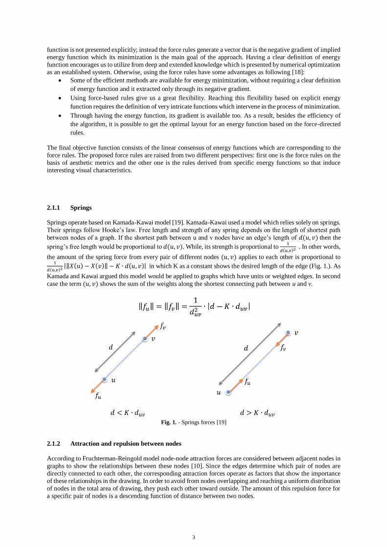
Fig. A.15. Large graphs produced by EC enlargement algorithm

Fig. A.16. Large graphs produced by MIVS enlargement algorithm

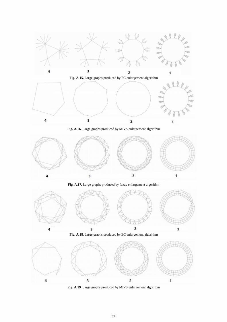
Fig. A.17. Large graphs produced by fuzzy enlargement algorithm

Fig. A.18. Large graphs produced by EC enlargement algorithm

Fig. A.19. Large graphs produced by MIVS enlargement algorithm

25

4. References

1. J. Zhang, The Interaction of Internal and External Representations in a Problem Solving Task, in Proceedings of the Thirteenth Annual Conference of Cognitive Science Society, 1991.

2. David Harel, On Visual Formalisms, Communications of the ACM, 31:514–530, May 1988.

3. Emmanuel G. Noik, A Space of Presentation Emphasis Techniques for Visualizing Graphs, In Proceedings of Graphics

Interface ’94, pages 225–233, 1994. 4. L. W. Beinekeand R. J. Wilson, eds., Graph Connections. Oxford University Press, 1997. 5. S. Hachul.A Potential-Field-Based Multilevel Algorithm for Drawing Large Graphs. PhD thesis, Institut fur Informatik,

Universit¨at zu K ̈oln, Germany, 2005. 6. C. THOMASSEN, The Jordon-Schoenflies Curve Theorem and the classification of surfaces. Amer. Math. Monthly,

99:116-130, 1992.

7. K. Sugiyama, S. Tagawa, and M. Toda, “Methods for Visual Understanding of Hierarchical System Structures,” IEEE Transactions on Systems, Man, and Cybernetics, vol. 11, no. 2, 1981.

8. E. Gansner, S. North, and K. Vo, “DAG—A Program that Draws Directed Graphs,” Software Practice and Experience, vol. 18, no. 11, pp. 1047-1062, 1988.

9. N. Robertson, D. Sanders, P. Seymour, and R. Thomas, the four-colour theorem. J. Combin. Theory Ser. B, 70(1):2-44, 1997.

10. T. Fruchterman and E. Reingold, Graph drawing by force-directed placement, Software-Practice and Experience 21 (1991), no. 11, 1129-1164.

11. W. Tutte, “How to Draw a Graph,” in Proceedings of the London Mathematical Society, vol. 13, no. 3, pp. 743-768, 1963. 12. C. Walshaw, “A Multilevel Algorithm for Force-Directed Graph Drawing,” Journal of Graph Algorithms and

Applications, 7(3), 2003 pp. 253–285. 13. P. Eades. A heuristic for graph drawing. Congressus Numerantium, 42:149-160, 1984. 14. J. Kruskal and J. Seery. Designing network diagrams. In Proc. First General Conf. on Social Graphics, pages 22-50, 1980.

15. Gajer, P., Goodrich, M. T., and Kobourov, S. G., “A multi-dimensional approach to force-directed layouts of large graphs,” Computational Geometry: Theory and Applications, Vol. 29(1), 2004, pp. 3 – 18.

16. Hu, Yifan. "Efficient, high-quality force-directed graph drawing." Mathematica Journal 10.1 (2005): 37-71 17. B. Hendrickson and R. Leland, “A Multilevel Algorithm for Partitioning Graphs,” Technical Report SAND93-1301,

Albuquerque, NM: Sandia National Laboratories, 1993. Also in Proceeding of Supercomputing’95 (SC95), San Diego. 18. J. Ignatowicz, “Drawing Force-Directed Graphs using Optigraph,” in [GD95], pp. 333-336.

19. T. Kamada and S. Kawai, “An Algorithm for Drawing General Undirected Graphs,” Information Processing Letters, vol. 31, pp. 7-15, 1989.

20. Koren, Yehuda, and Ali Civril. "The binary stress model for graph drawing." Graph Drawing. Springer Berlin Heidelberg, 2009.

21. Andreas Noack. An Energy Model for Visual Graph Clustering. In Proceedings of the 11th International Symposium on Graph Drawing (GD 2003), LNCS 2912, pages 425-436.

22. D. Hearn and M. P. Baker, Computer Graphics, Prentice-Hall, Englewood Cliffs, NJ, 1986. A. Appel, ‘An efficient algorithm for many-body simulations’, SIAM Journal on Scientific and Statistical Computing, 6, (l), 85–103 (1985).

23. R. Fletcher, Practical Methods of Optimization, 2nd ed., New York: John Wiley & Sons, 2000.

24. C. Walshaw, M. Cross, and M. G. Everett, “Parallel Dynamic Graph Partitioning for Adaptive Unstructured Meshes,”

Journal of Parallel and Distributed Computing, 47(2), 1997 pp. 102–108 25. A. Gupta, G. Karypis, and V. Kumar, “Highly Scalable Parallel Algorithms for Sparse Matrix Factorization,” IEEE

Transactions on Parallel and Distributed Systems, 8(5), 1997 pp. 502–520 26. Y. F. Hu and J. A. Scott, “A Multilevel Algorithm for Wavefront Reduction,” SIAM Journal on Scientific Computing,

23(4), 2001 pp.1352–1375. 27. C. Walshaw, “A Multilevel Approach to the Travelling Salesman Problem,” Operations Research, 50(5), 2002 pp. 862–

877. 28. C. Walshaw, “Multilevel Refinement for Combinatorial Optimisation Problems,” Annals of Operations Research, 131,

2004 pp. 325–372; originally published as University of Greenwich Technical Report01/IM/73, 2001. 29. D. Harel and Y. Koren, “A Fast Multi-Scale Method for Drawing Large Graphs,” Journal of Graph Algorithms and

Applications, 6(3), 2002 pp. 179–202. 30. R. Hadany and D. Harel, “A Multi-Scale Algorithm for Drawing Graphs Nicely,” Discrete Applied Mathematics, 113(1),

2001 pp. 3–21.

26

31. S. T. Barnard and H. D. Simon, “A Fast Multilevel Implementation of Recursive Spectral Bisection for Partitioning Unstructured Problems,” Concurrency: Practice and Experience, 6(2), 1994 pp. 101–117.

32. D. Ron, Sh. Wishko-Stern, A. Brandt, An Algebraic Multigrid Based Algorithm for Bisectioning General Graphs, Technical Report MCS05-01, 2005.