Efficient Fabrication of Stable Graphene‐Molecule‐Graphene ...
Graphene Non-Linear Characteristics and
Applications in Communications
Final Report

Document: Final report Graphene Non-Linear
Characteristics and
Applications in Communications
Date: 1/06/2015
Rev: 05
Page 2 of 33
REVISION HISTORY AND APPROVAL RECORD
Revision Date Purpose
0 21/05/2015 Document creation
1 24/05/2015 Contents, Document Scope, Set-up 2
2 28/05/2015 Set-up 1, Graphene deposition, Graphene characterization
3 29/05/2015 Set-up 3, executive summary, time plan updated
4 30/05/2015 Results, discussions and conclusions
5 01/06/2015 Final review
DOCUMENT DISTRIBUTION LIST
Name E-mail
Josep Maria Fargas Cabanillas [email protected]
Diego Monserrat López [email protected]
José Antonio Lázaro [email protected]
WRITTEN BY:
REVIEWED AND APPROVED BY:
Date 01/06/2015 Date 01/06/2015
Name Josep Maria Fargas Cabanillas Name José Antonio Lázaro
Diego Monserrat López
Position Project members Position Project advisor

Document: Final report Graphene Non-Linear
Characteristics and
Applications in Communications
Date: 1/06/2015
Rev: 05
Page 3 of 33
0. CONTENTS 0. Contents ................................................................................................................................... 3 1. Document scope ....................................................................................................................... 4 2. Executive summary ................................................................................................................... 5 3. Time plan updated .................................................................................................................... 6 4. System design documentation .................................................................................................. 7
4.1. Set-up 1: Measure non-Linear dependence on transmission coefficient with incident intensity. ....................................................................................................................................... 7
4.1.1. Objective ....................................................................................................................... 7
4.1.2. Theoretical view ............................................................................................................ 7
4.1.3. System block diagram ................................................................................................... 8
4.1.4. System blocks bridged final design................................................................................ 9
4.2. Set-up 2: Measure time dependence of non-Linear transmission coefficient ................. 12
4.2.1. Objective ..................................................................................................................... 12
4.2.2. Theoretical view .......................................................................................................... 12
4.2.3. System block diagram ................................................................................................. 13
4.2.4. System block bridged final design ............................................................................... 14
4.3. Set-up 3: Using graphene as a polarizer ....................................................................... 17
4.3.1. Objective ..................................................................................................................... 17
4.3.2. Theoretical view .......................................................................................................... 17
4.3.3. System block diagram ................................................................................................. 17
4.3.4. System blocks bridged final design.............................................................................. 17 5. System implementation documentation ................................................................................... 19
5.1. Graphene deposition ..................................................................................................... 19
5.2. Set-up 1: Measure non-Linear dependence on transmission coefficient with incident intensity. ..................................................................................................................................... 21
5.2.1. Final schematics .......................................................................................................... 21
5.3. Set-up 2: Measure time dependence of non-Linear transmission coefficient. ................ 22
5.3.1. Final schematics .......................................................................................................... 22
5.4. Set-up 3: Using graphene as a polarizer. ...................................................................... 24
5.4.1. Final schematics .......................................................................................................... 24 6. System characterization .......................................................................................................... 25
6.1. Graphene characterization. ........................................................................................... 25
6.1.1. Microscopic view and characterization ........................................................................ 25
6.2. Set-up 1: Measurements and results. ............................................................................ 26
6.2.1. Results ........................................................................................................................ 26
6.2.2. Discussion ................................................................................................................... 27
6.3. Set-up 2: Measurements and results. ............................................................................ 28
6.3.1. Results ........................................................................................................................ 28
6.3.2. Discussion ................................................................................................................... 28
6.4. Set-up 3: Measurements and results ............................................................................. 28
6.4.1. Results ........................................................................................................................ 28
6.4.2. Discussion ................................................................................................................... 30 7. Conclusions ............................................................................................................................ 31 8. Reflection document ............................................................................................................... 32 9. References ............................................................................................................................. 33

Document: Final report Graphene Non-Linear
Characteristics and
Applications in Communications
Date: 1/06/2015
Rev: 05
Page 4 of 33
1. DOCUMENT SCOPE
The remarkable optical and electronic properties of graphene is leading to disruptive photonic
applications as plasmonics [1], microwave photonics phase shifters [2], antennas [3]. Non-linear
characteristics of graphene derived from its particular quantum properties open a new field for
applications. Although some authors have found that nonlinear of the performance metrics as
nonlinear medium is found to be superior the existing nonlinear optical materials [4], it combines a
lot of properties in the same material, it compactness and high speed open the door to new high
speed and compact devices for communications [5-7].
The goal of this document is to show an experimental attempt to measure non-lineal optical
properties in graphene such as saturation absorption and to find real applications of graphene in
communications. We will see three different set-ups and a graphene sample characterization. The
first set-up is an attempt to measure the saturation in absorption while changing the input power.
The second set-up is an attempt to see how absorption changes with a modulated input while
varying the input frequency. The third set-up is a fiber polarizer made with graphene.

Document: Final report Graphene Non-Linear
Characteristics and
Applications in Communications
Date: 1/06/2015
Rev: 05
Page 5 of 33
2. EXECUTIVE SUMMARY
Graphene optical all-fiber polarizer
J. A. Lazaro1, J. M. Fargas1, 2, D. Monserrat1, 2,
1. Universitat Politecnica de Catalunya; ETSETB Jordi Girona, 31; E-08034 Barcelona, Spain.
2. Universitat Politecnica Catalunya, ETSEIB, Av. Diagonal 647 E-08028 Barcelona, Spain.
Graphene has attracted a high level of research interest because of its exceptional electronic transport and optoelectronic properties which have great potential in applications in the fields of nanoelectronics and optical communications. We propose a graphene polarizer device that can be used for control the polarization through an optical fiber. The device consists in a glass and a fiber inside. Its surface is smoothed until the fiber core touches the external surface. Then we deposited a graphene layer on the external face in order to have light-matter interaction [6-7].
Fig. 1 System idea and its real implementation.
Graphene behaves as a quasi-conductor, so electric field which is tangent to its surface tends to drop to zero. However, unlike polarizers made from thin metal film, a graphene polarizer can support transverse electric-mode surface wave propagation due to its linear dispersion of Dirac electrons. This TE wave can be tuned by applying voltage to graphene layer [6].
The graphene apparatus created can be used as a linear polarizer, changing the input polarization we have obtained 15 dB between minimum and maximum transmission.

Document: Final report Graphene Non-Linear
Characteristics and
Applications in Communications
Date: 1/06/2015
Rev: 05
Page 6 of 33
3. TIME PLAN UPDATED
In Fig. 2 we can observe a Gantt chart explaining the time plan. We have been in the lab six times, every Wednesday from two to seven. At home we have interpret the results and studied theory.
Fig. 2 Gantt Chart

Document: Final report Graphene Non-Linear
Characteristics and
Applications in Communications
Date: 1/06/2015
Rev: 05
Page 7 of 33
4. SYSTEM DESIGN DOCUMENTATION
4.1. Set-up 1: Measure non-Linear dependence on transmission coefficient with incident intensity.
4.1.1. Objective
The objective of the first set-up is to measure the dependence of transmission coefficient with incident intensity due to the insertion of graphene between two optical fibers connection. This set-up intends to be a first approach to observe similar results to the explained in the following section (4.1.2.Theoritical view). Despite the differences in the experiment design due to the material limitations, as not having a pulsed laser.
4.1.2. Theoretical view
The non-linearity of the intensity transmission through graphene in function of the incident intensity to it is a phenomena already observed by different research in quite different environments. The idea is to understand what have been studied in this area, in order to construct a background that will help us to go forward the good direction in the designing of the set-ups and experiments, always taking into account our material and time limitations.
Graphene is a layer structured material with a single atom thickness per layer. Several studies reports the effects of light interaction with graphene. Specifically weak light absorption is studied within of the non-interacting massless Dirac fermions model, concluding it is independent of frequency and to have universal opacity π·α=2.3% (where α is the fine structure constant). This linear absorption arises from the graphene properties: two dimensional massless fermions and a conical band structure. However, coupling between photons and fermions in graphene under high intensity ultrashort laser pulse excitation does not follows the same behavior [8-9].
Ultrafast saturable absorption in graphene has been studied, proved and characterized experimentally. The graphene used has epitaxially grown on a transparent SiC substrate (semiconductor with a wide bandgap). With this synthesizing method it is possible to obtain graphene monolayers, so it is possible to compare the phenomena when the number of layers vary. The results are shown in Fig. 3.
Fig. 3 Transmittance dependence on incident intensity for different layers of graphene [9].
Document: Final report Graphene Non-Linear
Characteristics and
Applications in Communications
Date: 1/06/2015
Rev: 05
Page 8 of 33
Figura shows how transmittance depends on graphene layers number at low incident intensity following the commented theory (2.3% opacity by layer). However, at higher intensities, transmittance tends to be equal to 1 independently of the number of layers. It is because the ultrafast intraband c-c dynamics.
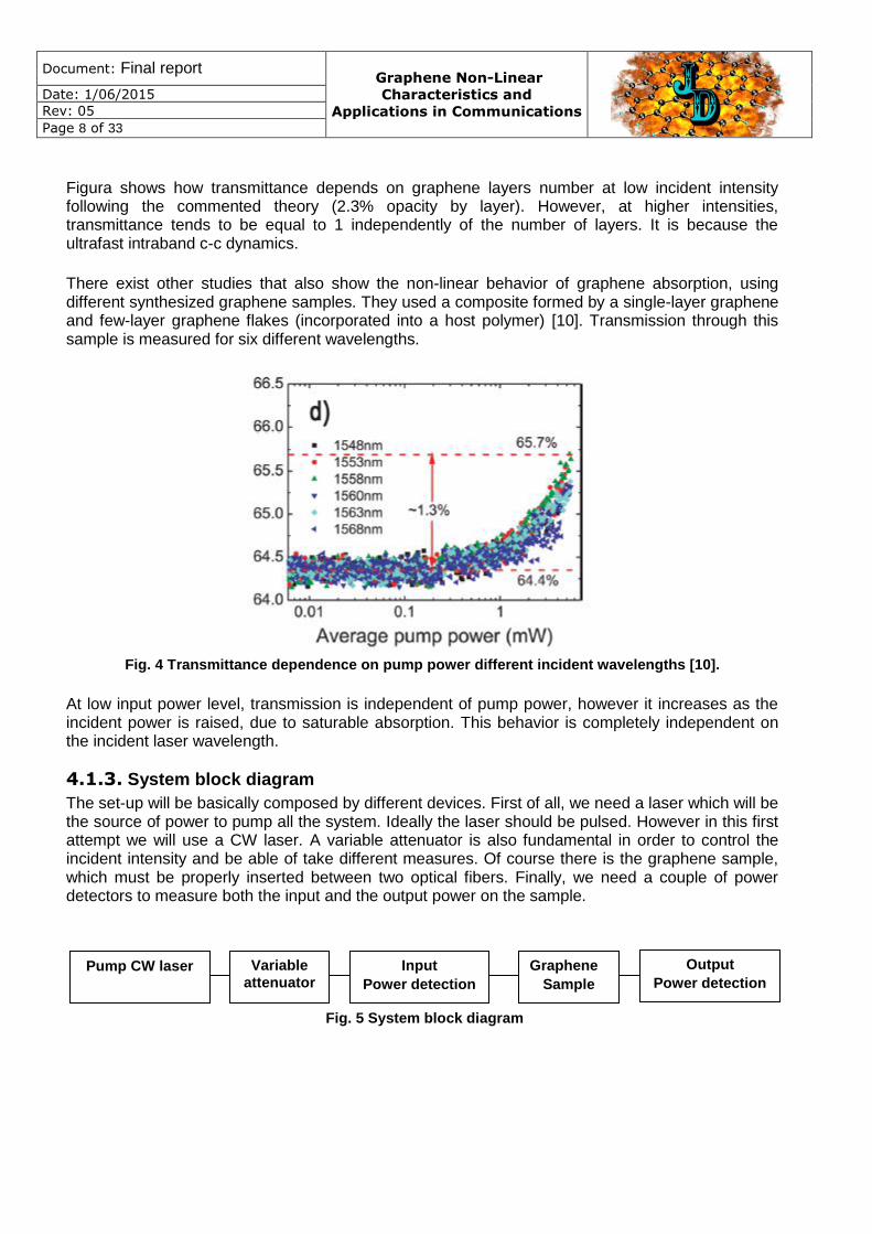
There exist other studies that also show the non-linear behavior of graphene absorption, using different synthesized graphene samples. They used a composite formed by a single-layer graphene and few-layer graphene flakes (incorporated into a host polymer) [10]. Transmission through this sample is measured for six different wavelengths.
Fig. 4 Transmittance dependence on pump power different incident wavelengths [10].
At low input power level, transmission is independent of pump power, however it increases as the incident power is raised, due to saturable absorption. This behavior is completely independent on the incident laser wavelength.
4.1.3. System block diagram
The set-up will be basically composed by different devices. First of all, we need a laser which will be the source of power to pump all the system. Ideally the laser should be pulsed. However in this first attempt we will use a CW laser. A variable attenuator is also fundamental in order to control the incident intensity and be able of take different measures. Of course there is the graphene sample, which must be properly inserted between two optical fibers. Finally, we need a couple of power detectors to measure both the input and the output power on the sample.
Pump CW laser Variable
attenuator Graphene
Sample
Input
Power detection
Output
Power detection
Fig. 5 System block diagram
Document: Final report Graphene Non-Linear
Characteristics and
Applications in Communications
Date: 1/06/2015
Rev: 05
Page 9 of 33
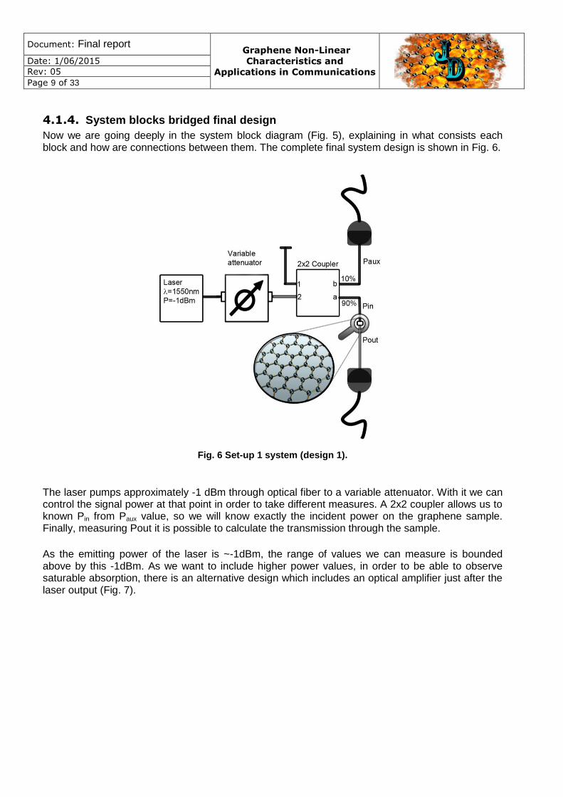
4.1.4. System blocks bridged final design
Now we are going deeply in the system block diagram (Fig. 5), explaining in what consists each block and how are connections between them. The complete final system design is shown in Fig. 6.
Fig. 6 Set-up 1 system (design 1).
The laser pumps approximately -1 dBm through optical fiber to a variable attenuator. With it we can control the signal power at that point in order to take different measures. A 2x2 coupler allows us to known Pin from Paux value, so we will know exactly the incident power on the graphene sample. Finally, measuring Pout it is possible to calculate the transmission through the sample.
As the emitting power of the laser is ~-1dBm, the range of values we can measure is bounded above by this -1dBm. As we want to include higher power values, in order to be able to observe saturable absorption, there is an alternative design which includes an optical amplifier just after the laser output (Fig. 7).
Document: Final report Graphene Non-Linear
Characteristics and
Applications in Communications
Date: 1/06/2015
Rev: 05
Page 10 of 33
Fig. 7 Set-up 1 system design 2.
In order to understand better the complete system, we give a brief description of the conceptual behavior of each component.
4.1.4.1. CW Laser
A continuous-wave laser is a device that emits a constant power of light. The main property of interest in a laser is the emitted light wavelength, which will be always 1550 nm in our case.
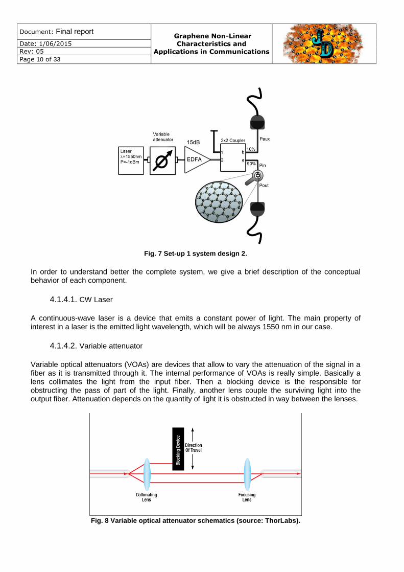
4.1.4.2. Variable attenuator
Variable optical attenuators (VOAs) are devices that allow to vary the attenuation of the signal in a fiber as it is transmitted through it. The internal performance of VOAs is really simple. Basically a lens collimates the light from the input fiber. Then a blocking device is the responsible for obstructing the pass of part of the light. Finally, another lens couple the surviving light into the output fiber. Attenuation depends on the quantity of light it is obstructed in way between the lenses.
Fig. 8 Variable optical attenuator schematics (source: ThorLabs).

Document: Final report Graphene Non-Linear
Characteristics and
Applications in Communications
Date: 1/06/2015
Rev: 05
Page 11 of 33
4.1.4.3. 2x2 Coupler
It is not a little issue when you need to measure the power going through an optical fiber which is in the middle of a system set-up. The way we found to do it was using a 90:10 2x2 coupler. It is a device with 2 optical fibers which cores are coupled in a specific way. Each fiber keeps 90% of its incident power on itself and sends the remainder 10% to the other one.
By using only one of its inputs we have to output fibers, with 9 dB of difference between them. The one with higher power will continue its way in the system set-up, meanwhile the other one goes to a power detector. Thus it is possible to know the power in any point of the system just knowing the difference between the coupler output fibers.
Fig. 9 90:10 2x2 coupler schematics (source: ThorLabs)
4.1.4.4. Power detector
As it name indicates, power detector are devices able to measure the power coming from an optical fiber. It is necessary to indicate the measured light wavelength.
4.1.4.1. EDFA Amplifier
An optical amplifier is a device that amplifies an optical signal directly, without converting it to an electrical signal first. Erbium doped fiber amplifiers (EDFA) are a particular case of optical amplifiers. A wavelength selective coupler mix the input signal and a high-powered excitation light (pumping), at considerably different wavelengths. The mixed light goes into a fiber doped with erbium ions, which are excited to their higher energy state due to the pumping photons (Pumping signal must be of 1480 nm or 980 nm). When the original signal photons interact with the excited erbium atoms, they receive some energy from the atoms which return to the low energy state. We can say that erbium atoms gives energy to the signal because the energy they release are photons with the same wavelength (1550 nm), phase and direction, so the additional power travels in the same fiber mode as the original signal.

Document: Final report Graphene Non-Linear
Characteristics and
Applications in Communications
Date: 1/06/2015
Rev: 05
Page 12 of 33
Fig. 10 EDFA schematics. Fig. 11 Erbium energy levels transitions.
The isulators placed both at the beginning and the output of the EDFA are for preventing reflections from the attached fibre. Reflections could disturb amplifier behaviour ans they could even create a resonance cavity which may convert the amplifier into a laser.
4.2. Set-up 2: Measure time dependence of non-Linear transmission coefficient
4.2.1. Objective
In this set-up 2, we are attempting to measure the transfer function in transmission by a graphene layer. At the end we want to see how fast is the system would behave.
4.2.2. Theoretical view
We should not forget the aim of this project. We want to measure the non-linear effect on transmission. As we have seen in the previously set-up 1 many people have reported this non-linear behave on absorption [8-10]. This non-linear effect can be thought in such an easy way. Graphene layer has a constant transmission but at some point it saturate. As we have seen this transmission depends on the input power. If we have low power graphene absorb part of this power. While we increase the input power the graphene become more transparent. Thus, the transmission goes to one. But how does it change with frequency? How fast is its response? Well a lot of people have studied that already [11-12]. Some people have used femtosecond (80 fs pulses) Z-scan and degenerate pump-probe spectroscopy at 790 nm. They have demonstrated saturable absorptions property of graphene with a nonlinear absorption coefficient, β, of ~2 to 9e.8 cm/W. Two distinct time scales associated with the relaxation of photo-excited carriers, a fast one in the range of 130-330fs (related to carrier-carrier scattering) followed by a slower one in 3.5-4.9ps range (associated with carrier-phonon scattering) [11].

Document: Final report Graphene Non-Linear
Characteristics and
Applications in Communications
Date: 1/06/2015
Rev: 05
Page 13 of 33
We thought that could be interesting to measure the behavior of graphene when a sinusoidal pumping is applied. Once we can see the effect for different frequencies, we would reconstruct the transfer function of the system as in a control theory problem. This could be really useful for communication, because we will have our system as a black-box. We will be able to forget about graphene itself and we will start thinking about this system as something which has a function that affects at the input and gives an output.
We know that we are not able to achieve such fast modulation. But at least he presents a way to measure a long range of frequencies, 250 kHz-3GHz. At high frequency we are in the times range of 333ps. This should be enough to see some effects.
4.2.3. System block diagram
Basically we need a laser to pump our sample. This laser should give a constant power. After that we need to modulate this laser in order to get a desired sinusoidal. After that we just have to track the input power and the power after the sample.
Pump CW laser Modulator Graphene
Sample
Input
Power detection
Output
Power detection
Fig. 13 System block diagram
Fig. 12 Interaction graphene light at deferent frequencies.

Document: Final report Graphene Non-Linear
Characteristics and
Applications in Communications
Date: 1/06/2015
Rev: 05
Page 14 of 33
4.2.4. System block bridged final design
Now we are going to go through every element from Fig. 13 and we will explain each block in more detail. We want to see how the input power is. Therefore in Fig. 14 we can see the set-up for the first three boxes: laser, modulator, input power detection.
The laser pumps ~ -1dBm though optical fiber, after that we have polarization controller that allows us to control the polarization in order to optimize the modulator. Once the beam has changed the polarization goes into the Mach-Zehnder modulator (MZM). This device allows us to modulate the light beam through an electrical signal. Therefore we need a function generator which will generate a sinusoidal signal. In order to control the offset of this signal we will need an external DC voltage source. Using a LC coupler we can add the two independent electrical signals. Finally we have at the electrical input of the MZM a signal which we can chose, frequency, amplitude and off-set. In order to undersant better the behaveor of our system we will explain briefly the polarizer controller and MZM.
4.2.4.1. Polarizer controller
Controlling the polarization state in optical fiber is similar to the free space control using waveplates via phase changes in the two orthogonal states of polarization. In general, three configurations are commonly used.
In the first configuration, a Half-Wave Plate (HWP) is sandwiched between two Quarter-Wave Plates (QWP) and the retardation plates are free to rotate around the optical beam with respect to each other. The first QWP converts any arbitrary input polarization into a linear polarization. The HWP then rotates the linear polarization to a desired angle so that the second QWP can translate the linear polarization to any desired polarization sate.
Fig. 14 Laser modulator scheme.

Document: Final report Graphene Non-Linear
Characteristics and
Applications in Communications
Date: 1/06/2015
Rev: 05
Page 15 of 33
An all-fiber controller based on this mechanism can be constructed, with several desirable properties such as the low insertion loss and cost, as shown in Fig. 15. In this device, three fiber coils replace the three free-space retardation plates. Coiling the fiber induces stress, producing birefringence inversely proportional to the square of the coils diameter. Adjusting the diameters and number of turns can create any desired fiber wave plate. Because bending the fiber generally induces insertion loss, the fiber coils must remain relatively large.
Fig. 15 Polarization control using multiple coiled fiber (Source https://www.newport.com/Tutorial-
Polarization-in-Fiber-Optics/849671/1033/content.aspx).
In order to build the polarization controller the number of turns on each paddle has to be considered. Thor Labs gives a plot Fig. 16 which makes this process really easy. We empathize that this type of polarization controller depends on the wave length. In future stages if we will work with a wider spectrum we must replace this polarization controller.
Fig. 16 Retardance per Paddle vs Wavelength and turns (source Thor Labs).
4.2.4.2. Mach-Zehender electro-optic modulator
A Mach-Zehnder modulator is used for controlling the amplitude of an optical wave. The input waveguide is split up into two waveguide interferometer arms. If a voltage is applied across one of the arms, a phase shift is induced for the wave passing through that arm. When the two arms are recombined, the phase difference between the two waves is converted to an amplitude modulation.

Document: Final report Graphene Non-Linear
Characteristics and
Applications in Communications
Date: 1/06/2015
Rev: 05
Page 16 of 33
Fig. 17 Contains an isometric view of a prior art single-ended Mach-Zehnder modulator 10. Modulator 10 is formed in an opto-electronic substrate 12 (for example, lithium niobate) and comprises an input waveguide section 14 including a 3 dB coupler that splits the waveguide into a pair of parallel waveguide arms 16, 18. Waveguide arms 16 and 18 are formed to comprise a predetermined length L, where the individual arms then recombine into an output waveguide section 20. In order to provide the modulator function, an input laser device (not shown) is used to launch a continuous wave (CW) input optical signal into input waveguide section 14. A modulation input (data) signal (i.e., an electrical RF signal) from an RF source 23 is provided as the RF input to modulate the CW input optical signal and produce a data-encoded optical output signal. In particular, prior art modulator 10 is formed to include a first electrode 22 disposed on surface 24 of substrate 12 so as to overly parallel waveguide arm 16. The remaining area of top surface 24 is covered with a ground electrode 26, except for isolation regions28 and 29, used to maintain electrical isolation between electrodes 22 and 26. Therefore, as shown in FIG. 1, ground plane electrode 26 will overly second waveguide arm 18 of the pair of waveguide arms. First electrode 22 is electrically connected to RF signal source 23, thus providing for the modification of the electric fields along the length of first waveguide arm 16and second waveguide arm 18 [13].
It is important to know that depending on the bias voltage, the amplitude of the integral will be different.
We want to work in the linear regime. Not working in the linear regime will raise saturations effects in the output. The polarization also affects on the output amplitude.
Fig. 17. Artistic view of MZM (source http://www.google.com/patents/US6501867) [13].
Fig. 18 MZM transfer function [14].
Document: Final report Graphene Non-Linear
Characteristics and
Applications in Communications
Date: 1/06/2015
Rev: 05
Page 17 of 33
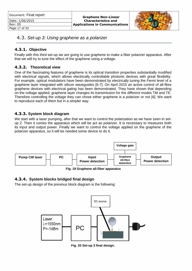
4.3. Set-up 3: Using graphene as a polarizer
4.3.1. Objective
Finally with this third set-up we are going to use graphene to make a fiber polarizer apparatus. After that we will try to tune the effect of the graphene using a voltage.
4.3.2. Theoretical view
One of the fascinating features of graphene is its optical transition properties substantially modified with electrical signals, which allows electrically controllable photonic devices with great flexibility. For example, optical modulators have been demonstrated by electrically tuning the Fermi level of a graphene layer integrated with silicon waveguides [6-7]. On April 2015 an active control of all-fibre graphene devices with electrical gating has been demonstrated. They have shown that depending on the voltage applied, graphene layer changes its transmission for the different modes TM and TE. Therefore controlling the voltage they can chose either graphene is a polarizer or not [6]. We want to reproduce each of them but in a simpler way.
4.3.3. System block diagram
We start with a laser pumping, after that we want to control the polarization as we have seen in set-up 2. Then it comes the apparatus which will be act as polarizer. It is necessary to measures both its input and output power. Finally we want to control the voltage applied on the graphene of the polarizer apparatus, so it will be needed some device to do it.
4.3.4. System blocks bridged final design
The set-up design of the previous block diagram is the following:
Fig. 20 Set-up 3 final design.
Pump CW laser PC Graphene
All-fibre apparatus
Input
Power detection
Output
Power detection
Voltage gate
Fig. 19 Graphene all-fiber apparatus

Document: Final report Graphene Non-Linear
Characteristics and
Applications in Communications
Date: 1/06/2015
Rev: 05
Page 18 of 33
We have a device made of glass crossed by an optical fiber which will be the basis of the graphene based polarized. The glass surface has been smoothed until reaching the fiber core. Then we deposited a graphene layer on the external face, so we have light-matter interaction. If the graphene layer acts as a conductor then we will have a polarizer because the electrical field which is tangent to graphene surface will go to zero. However it is more likely a semimetal, so it can support transverse elecevtric modesurface wave propagation due to its linear of Dirac electrons.
The best way found for applying voltage to graphene is to use a couple of needle puncturing the graphene layer, which are connected to a voltage source.

Document: Final report Graphene Non-Linear
Characteristics and
Applications in Communications
Date: 1/06/2015
Rev: 05
Page 19 of 33
5. SYSTEM IMPLEMENTATION DOCUMENTATION
5.1. Graphene deposition
The most important part in all the setups is the graphene deposition. In set-up 1 and set-up 2 we deposited graphene on the fiber connector (Fig. 21) and in set-up 3 we deposited graphene on the glass apparatus (Fig. 22). Our graphene comes from Graphenea. We have a graphene oxide 4mg/mL solution. The technique we are using is evaporation [8,12,15]. Basically we put a graphene oxide drop on the apparatus surface and we wait until the water is evaporated. We tried different drops once bigger than others. Once the drop is on the surface we have two options, we can just wait or we can put a cover slip in order to spread the drop and get a thinner layer. We have tried the two ways and we got different results.
Fig. 21 Optical fiber with graphene deposition. (x200)
Fig. 22 Graphene deposition on set-up 3

Document: Final report Graphene Non-Linear
Characteristics and
Applications in Communications
Date: 1/06/2015
Rev: 05
Page 20 of 33
Graphenea gives us a detailed datasheet of their product. We can see in the following table its main properties.
Form Dispersion of graphene oxide
Sheet dimension Variable
Color Yellow-brown
Odor Odorless
Dispersibility Polar solvents
Concentration 4mg/mL
Monolayer content (measured in 0.5mg/mL) >95%*
pH 2,2-2,5
(*) $mg/ml concentration tends to agglomerate the GO flakes and dilution followed by slight sonication is required in order to obtain a higher percentage of monolayer flakes.
They also provide a SEM,TEM and XPS, see Fig. 23. This images show that graphene monolayers are really small. The perfect sample would be a single graphene monolayer on the fiber core. Although they offer this possibility is more expensive. So we started with this type of graphene in order to see what we can achieve.
Fig. 23 Graphene oxide sample (source Graphenea)
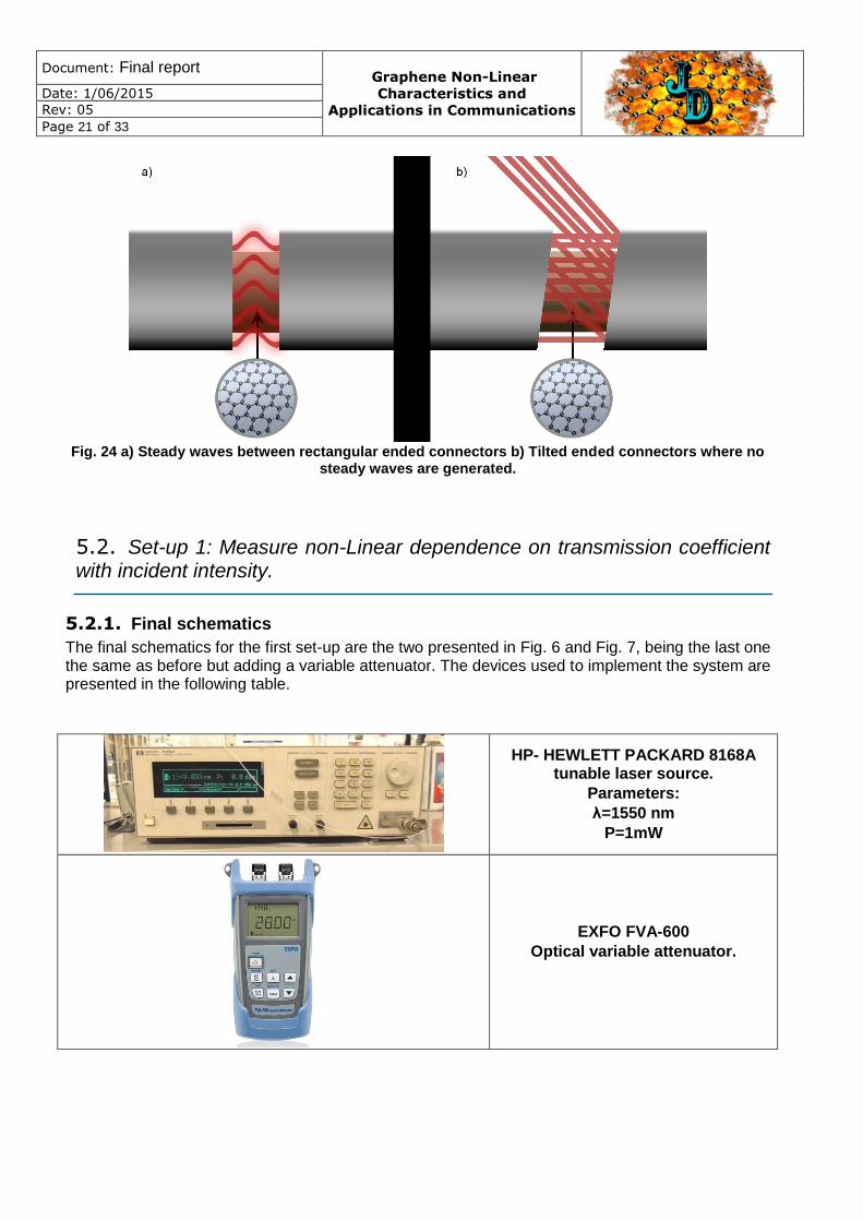
There is a crucial aspect to consider when doing graphene deposition in order to experiments become successful. It is the fiber connector type where sample is deposited. Basically there exist two different types: ones ending in rectangular angle and others with a slight tilted end.
When two fibers are connected by whatever connector, fibers are in contact between them. However, when a graphene sample is between them it avoids this contact. As we have seen when doing the first experiments, if rectangular ended connectors are used, output power measurements oscillates. The reason is the little distance between fibers acts as a cavity where steady waves are confined. This problem is solved using tilted ended connectors (Fig. 24).
Document: Final report Graphene Non-Linear
Characteristics and
Applications in Communications
Date: 1/06/2015
Rev: 05
Page 21 of 33
Fig. 24 a) Steady waves between rectangular ended connectors b) Tilted ended connectors where no
steady waves are generated.
5.2. Set-up 1: Measure non-Linear dependence on transmission coefficient with incident intensity.
5.2.1. Final schematics
The final schematics for the first set-up are the two presented in Fig. 6 and Fig. 7, being the last one the same as before but adding a variable attenuator. The devices used to implement the system are presented in the following table.
HP- HEWLETT PACKARD 8168A tunable laser source.
Parameters:
λ=1550 nm
P=1mW
EXFO FVA-600
Optical variable attenuator.
Document: Final report Graphene Non-Linear
Characteristics and
Applications in Communications
Date: 1/06/2015
Rev: 05
Page 22 of 33
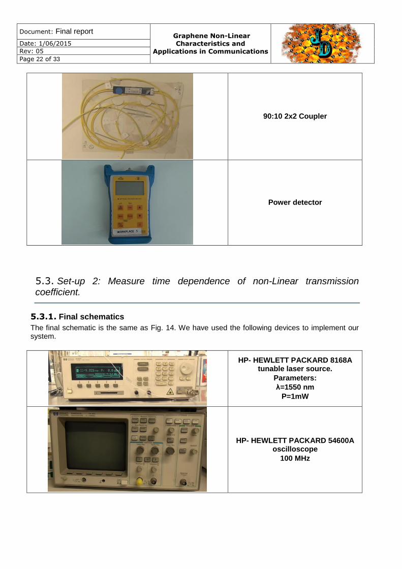
90:10 2x2 Coupler
Power detector
5.3. Set-up 2: Measure time dependence of non-Linear transmission coefficient.
5.3.1. Final schematics
The final schematic is the same as Fig. 14. We have used the following devices to implement our system.
HP- HEWLETT PACKARD 8168A tunable laser source.
Parameters:
λ=1550 nm
P=1mW
HP- HEWLETT PACKARD 54600A oscilloscope
100 MHz
Document: Final report Graphene Non-Linear
Characteristics and
Applications in Communications
Date: 1/06/2015
Rev: 05
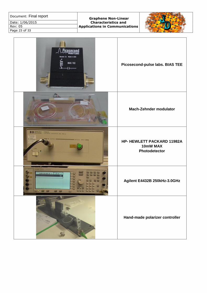
Page 23 of 33
Picosecond-pulse labs. BIAS TEE
Mach-Zehnder modulator
HP- HEWLETT PACKARD 11982A
10mW MAX
Photodetector
Agilent E4432B 250kHz-3.0GHz
Hand-made polarizer controller

Document: Final report Graphene Non-Linear
Characteristics and
Applications in Communications
Date: 1/06/2015
Rev: 05
Page 24 of 33
5.4. Set-up 3: Using graphene as a polarizer.
5.4.1. Final schematics
The final schematic is the same as Fig. 20 and the devices used to implement it are the followings:
HP- HEWLETT PACKARD 8168A tunable laser source.
Parameters:
λ=1550 nm
P=1mW
Power detector
Hand-made polarizer controller
Voltage source
Document: Final report Graphene Non-Linear
Characteristics and
Applications in Communications
Date: 1/06/2015
Rev: 05
Page 25 of 33
6. SYSTEM CHARACTERIZATION
6.1. Graphene characterization.
6.1.1. Microscopic view and characterization
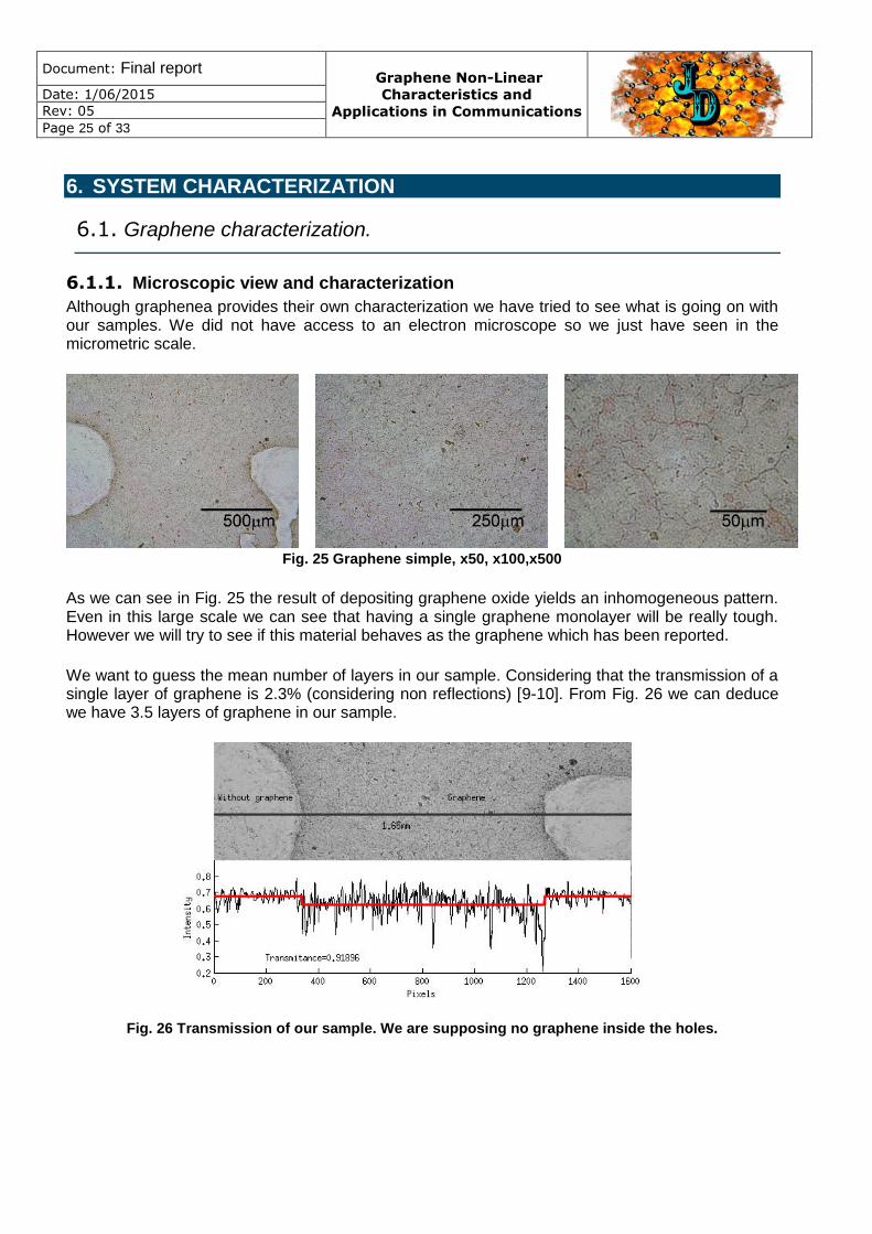
Although graphenea provides their own characterization we have tried to see what is going on with our samples. We did not have access to an electron microscope so we just have seen in the micrometric scale.
Fig. 25 Graphene simple, x50, x100,x500
As we can see in Fig. 25 the result of depositing graphene oxide yields an inhomogeneous pattern. Even in this large scale we can see that having a single graphene monolayer will be really tough. However we will try to see if this material behaves as the graphene which has been reported.
We want to guess the mean number of layers in our sample. Considering that the transmission of a single layer of graphene is 2.3% (considering non reflections) [9-10]. From Fig. 26 we can deduce we have 3.5 layers of graphene in our sample.
Fig. 26 Transmission of our sample. We are supposing no graphene inside the holes.

Document: Final report Graphene Non-Linear
Characteristics and
Applications in Communications
Date: 1/06/2015
Rev: 05
Page 26 of 33
6.2. Set-up 1: Measurements and results.
6.2.1. Results
The process of measurement consists in varying the incident power (Pin) to the graphene sample using the optical variable attenuator and register the output power (Pout). We also register Paux (see Fig. 6) in order to know the value of Pin.
First of all, it is necessary to do a calibration for having the real relation between Paux and Pin. Despite they are supposed to differ in a constant value of 9 dBm (due to the 90:10 2x2 Coupler), we consider necessary to carry out this calibration.
Fig. 27 Calibration of Pin in function of Paux.
A linear minimum square regression of the measurements shows the following dependence:
Once calibration is fulfilled, we carry out the measurements with the complete set-up. It is only necessary to use the design which include the amplifier because with the attenuator is possible to go until as low power values as we want.
Transmittance is defined as:

Document: Final report Graphene Non-Linear
Characteristics and
Applications in Communications
Date: 1/06/2015
Rev: 05
Page 27 of 33
We measure optical in dBm, which are defined as:
So transmittance is calculated as:
Taking into account the previous calibration, the final expression is:
We carry out the measurements for 4 different graphene samples, in Fig. 28 it is plotted the transmittance in function of the incident power for each one.
Fig. 28 Transmittance vs. incident power for different graphene samples.
6.2.2. Discussion
Black and blue graphs, the second one corresponding to a thinker graphene sample, shows an evident constant transmittance. Saturable absorption phenomena is not observed. There are two main issues that explained why. On one hand, probably it is needed a high incident power for observing that phenomena and, on the other hand, probably it is not possible to observe it by using a continuous laser source instead of a pulsed one.

Document: Final report Graphene Non-Linear
Characteristics and
Applications in Communications
Date: 1/06/2015
Rev: 05
Page 28 of 33
The reason why it has been impossible to go higher in the incident power is shown in Fig. 29.
Fig. 29 Original graphene sample and its destruction representation.
Once an input power around 13 dBm, graphene sample is absolutely destroyed just in the fiber core position. When it happens, it is immediately detected because Pout measurement decays considerably due to the bad connection between both fibers when there is a holes in the graphene sample. The fact that the laser emission is continuous contribute to this destruction, because the sample is not able to dissipate all this energy.
Green and red graphs correspond to samples that we used only to observe the phenomena of destruction of them. We let these samples submitted to the laser during more time in each measurement than in the other experiments and actually they were destroyed at lower incident powers.
6.3. Set-up 2: Measurements and results.
6.3.1. Results
We wanted to see the non-linearity while changing the frequency. As we have seen in Set-up 1 we need more than 40dB (from 0dBm to 40dBm) to see non-linear effects. And even if we achieve such big powers, our graphene can just evaporate. We achieved in the modulated input 4.5dB from the minimum to the maximum, therefore we cannot continue with this set-up.
6.3.2. Discussion
This approach did not bring any result. However, we think if we can increase the amplitude to 10dB and centering the bias to a non-linear point without burning the graphene we could see some modulation.
6.4. Set-up 3: Measurements and results
6.4.1. Results
First of all, we carry out measurements to the original apparatus before adding graphene to it. The measure consists in applying a fixed input power and register the output power value while varying input light polarization. The maximum variation in the output power in this case is about 0.3 dBm.
Once graphene is added to the apparatus we carry out measurements again, first without applying any voltage to graphene. Our hand-made polarization controller allows to change polarization but
Document: Final report Graphene Non-Linear
Characteristics and
Applications in Communications
Date: 1/06/2015
Rev: 05
Page 29 of 33
we do not know how it is in each moment. Therefore, the only values of interest are the minimum and maximum. For an input power of -2.94 dBm these values are:
Minimum Pout: -30.75 dBm
Maximum Pout: -15.1 dBm
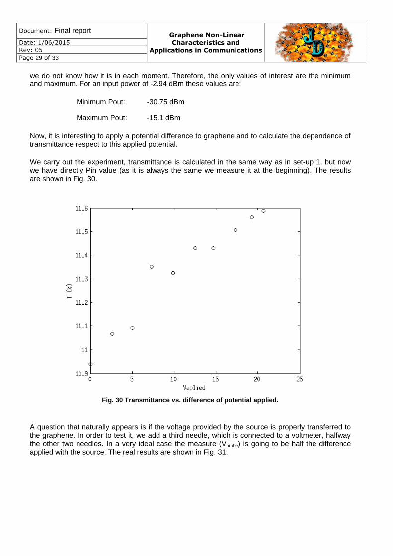
Now, it is interesting to apply a potential difference to graphene and to calculate the dependence of transmittance respect to this applied potential.
We carry out the experiment, transmittance is calculated in the same way as in set-up 1, but now we have directly Pin value (as it is always the same we measure it at the beginning). The results are shown in Fig. 30.
Fig. 30 Transmittance vs. difference of potential applied.
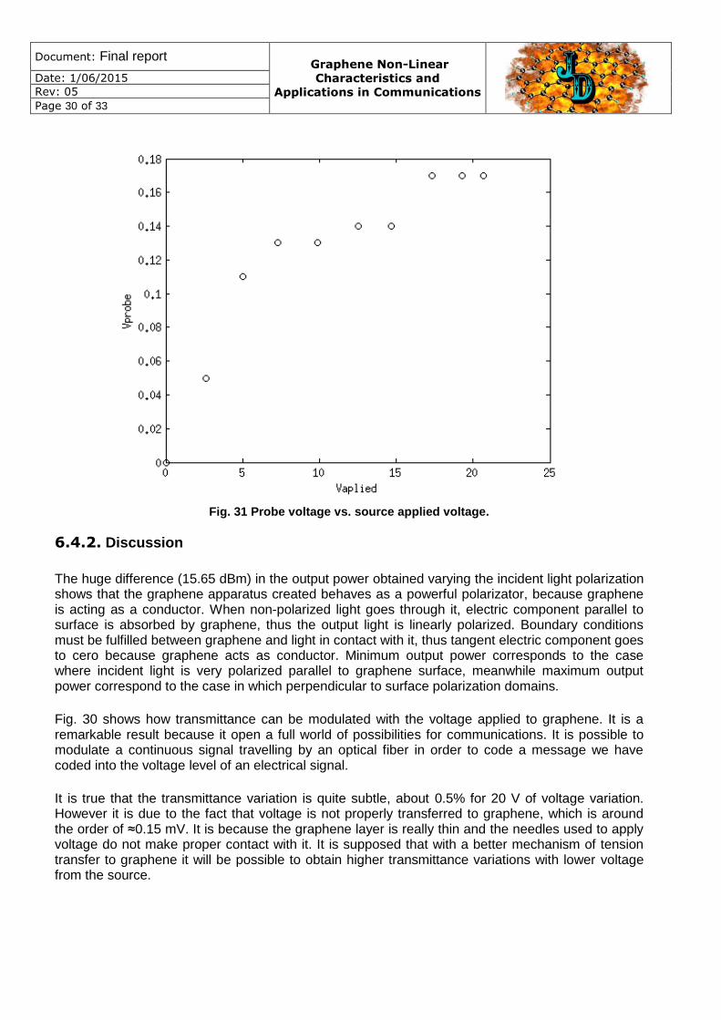
A question that naturally appears is if the voltage provided by the source is properly transferred to the graphene. In order to test it, we add a third needle, which is connected to a voltmeter, halfway the other two needles. In a very ideal case the measure (Vprobe) is going to be half the difference applied with the source. The real results are shown in Fig. 31.
Document: Final report Graphene Non-Linear
Characteristics and
Applications in Communications
Date: 1/06/2015
Rev: 05
Page 30 of 33
Fig. 31 Probe voltage vs. source applied voltage.
6.4.2. Discussion
The huge difference (15.65 dBm) in the output power obtained varying the incident light polarization shows that the graphene apparatus created behaves as a powerful polarizator, because graphene is acting as a conductor. When non-polarized light goes through it, electric component parallel to surface is absorbed by graphene, thus the output light is linearly polarized. Boundary conditions must be fulfilled between graphene and light in contact with it, thus tangent electric component goes to cero because graphene acts as conductor. Minimum output power corresponds to the case where incident light is very polarized parallel to graphene surface, meanwhile maximum output power correspond to the case in which perpendicular to surface polarization domains.
Fig. 30 shows how transmittance can be modulated with the voltage applied to graphene. It is a remarkable result because it open a full world of possibilities for communications. It is possible to modulate a continuous signal travelling by an optical fiber in order to code a message we have coded into the voltage level of an electrical signal.
It is true that the transmittance variation is quite subtle, about 0.5% for 20 V of voltage variation. However it is due to the fact that voltage is not properly transferred to graphene, which is around the order of ≈0.15 mV. It is because the graphene layer is really thin and the needles used to apply voltage do not make proper contact with it. It is supposed that with a better mechanism of tension transfer to graphene it will be possible to obtain higher transmittance variations with lower voltage from the source.
Document: Final report Graphene Non-Linear
Characteristics and
Applications in Communications
Date: 1/06/2015
Rev: 05
Page 31 of 33
7. CONCLUSIONS
Saturable absorption has not been observed in our graphene sample. Lasers pulses should be required in order to measure non-linear effects properly. This will allow us to increase the incident intensity, which has been one of our principle limitations. We have had troubles overheating the samples. A possibility to consider is to use different type of graphene samples, maybe by using a different deposition method or purchasing Graphenea prepared samples.
http://www.graphenea.com/products/monolayer-graphene-on-your-substrate
Nevertheless, demonstration of a self-made polarizer apparatus has been a success. It is a first step for future improvements in this device, as well as finding new applications. For example, someone can try to put an ionic solution onto graphene in order to improve conductivity when applying a voltage. This could allow us to create a signal modulator from the polarizer apparatus.

Document: Final report Graphene Non-Linear
Characteristics and
Applications in Communications
Date: 1/06/2015
Rev: 05
Page 32 of 33
8. REFLECTION DOCUMENT
The original project porpoise was actually an adventure, because we unknown if it was going to be possible to achieve the aims. However, it has a good aspect, which is that we had to be imaginative and resolute meanwhile developing the project. This project could not been possible without our advisor, who provided the facilities and knowledge which have been required.
The final report format has been really helpful in order to put in order all the work carried out. It will also help to share all the knowledge achieved with future generations who desire to continue the project.

Document: Final report Graphene Non-Linear
Characteristics and
Applications in Communications
Date: 1/06/2015
Rev: 05
Page 33 of 33
9. REFERENCES
[1] Oleg Mitrofanov, Wenlong Yu, Robert J. Thompson, Yuxuan Jiang, Igal Brener, Wei Pan, Claire Berger,
Walter A. de Heer and Zhigang Jiang; Probing terahertz surface plasmon waves in graphene structures;
Applied Physics Letters; 103, 111105 (2013).
[2] Mattia Pagani, David Marpaung, Duk-Yong Choi, Steve J. Madden, Barry Luther-Davies, and Benjamin
J. Eggleton, Tunable wideband microwave photonic phase shifter using on-chip stimulated Brillouin
scattering, Opt. Express 22, 28810-28818 (2014).
[3] Ignacio Llatsera, Christian Kremersb, Albert Cabellos-Aparicioa, Josep Miquel Jornetc, Eduard Alarcóna,
Dmitry N. Chigrinb; Graphene-based nano-patch antenna for terahertz radiation; Photonics and
Nanostructures – Fundamentals and Applications; vol. 10 pp. 353-358 (October 2012).
[4] Khurgin, J. B.; Graphene-A rather ordinary nonlinear optical material; Applied Physics Letters; 104,
161116 (2014).
[5] Ming Liu, Xiaobo Yin, Erick Ulin-Avila, Baisong Geng, Thomas Zentgraf, Long Ju, Feng Wang & Xiang
Zhang; A graphene-based broadband optical modulator; Nature 474 64-67 (02 June 2011).
[6] Eun Jung Lee, Sun Young Choi, Hwanseong Jeong, Nam Hun Park, Woongbin Yim, Mi Hye Kim, Jae-Ku
Park, Suyeon Son, Sukang Bae, Sang Jin Kim, Kwanil Lee, Yeong Hwan Ahn, Kwang Jun Ahn, Byung Hee
Hong, Ji-Yong Park, Fabian Rotermund & Dong-Il Yeom; Active control of all-fibre graphene devices with
electrical gating; Nature Communications 6, art. 6851 (April 2015).
[7] Qiaoliang Bao, Han Zhang, Bing Wang, Zhenhua Ni, Candy Haley Yi Xuan Lim, Yu Wang, Ding Yuan
Tang & Kian Ping Loh; Broadband graphene polarizer; Nature Photonics 5, 411–415 (2011).
[8] Yanyan Feng, Ningning Dong, Yuanxin Li, Xiaoyan Zhang, Chunxia Chang, Saifeng Zhang, and Jun
Wang; Host matrix effect on the near infrared saturation performance of graphene absorbers; Optical
Materials Express vol. 5 pp.802-808 (2015).
[9] Guichuan Xing, Hongchen Guo, Xinhai Zhang, Tze Chien Sum, and Cheng Hon Alfred Huan; The
Physics of ultrafast saturable absorption in graphene; Opt. Express 18, 4564-4573 (2010).
[10] Zhipei Sun, Tawfique Hasan, Felice Torrisi, Daniel Popa, Giulia Privitera, Fengqiu Wang, Francesco
Bonaccorso, Denis M. Basko and Andrea C. Ferrari; Graphene Mode-Locked Ultrafast Laser; ACS Nano 4
pp.803-810 (2010).
[11] Kumar, Sunil and Anija, M. and Kamaraju, N. and Vasu, K. S. and Subrahmanyam, K. S. and Sood, A.
K. and Rao C. N. R.; Femtosecond carrier dynamics and saturable absorption in graphene suspensions;
Applied Physics Letters, 95, 191911 (2009).
[12] Chen, Ke and Li, Huihui and Ma, Lai-Peng and Ren, Wencai and Zhou, Jian-Ying and Cheng, Hui-Ming
and Lai, Tianshu;; Ultrafast linear dichroism-like absorption dynamics in graphene grown by chemical vapor
deposition; Journal of Applied Physics 115, 203701 (2014).
[13] Lucent Technologies Inc.; Chirp compensated Mach-Zehnder electro-optic modulator; Patent
US6501867 (Dec 31, 2002).
[14] Borja Vidal, Juan L. Corral, and Javier Martí; All-optical WDM multi-tap microwave filter with flat
bandpass; Opt. Express 14, 581-586 (2006).
[15] Yenny Hernandez, Valeria Nicolosi, Mustafa Lotya, Fiona M. Blighe, Zhenyu Sun, Sukanta De, I. T.
McGovern, Brendan Holland, Michele Byrne, Yurii K. Gun'Ko, John J. Boland, Peter Niraj, Georg Duesberg,
Satheesh Krishnamurthy, Robbie Goodhue, John Hutchison, Vittorio Scardaci, Andrea C. Ferrari6 &
Jonathan N. Coleman; High-yield production of graphene by liquid-phase exfoliation of graphite; Nature
Nanotechnology 3, 563-568 (2008).


![MQOI(OI-EPSEB) Introduccion [Modo de compatibilidad]ocw.upc.edu/sites/ocw.upc.edu/files/materials/26504/2011/1/53905/... · Problemas de Colas (I) Ciertas unidades (iguales o de clases](https://static.fdocuments.in/doc/165x107/5ba435d509d3f2205e8cdf31/mqoioi-epseb-introduccion-modo-de-compatibilidadocwupcedusitesocwupcedufilesmaterials265042011153905.jpg)