7/27/2019 Graphene Coupler

http://slidepdf.com/reader/full/graphene-coupler 1/5

PHYSICAL REVIEW B 88, 045443 (2013)

Nonlinear switching with a graphene coupler

Daria A. Smirnova,1 Andrey V. Gorbach,2 Ivan V. Iorsh,3 Ilya V. Shadrivov,1 and Yuri S. Kivshar1,3

1 Nonlinear Physics Center, Research School of Physics and Engineering, Australian National University, Canberra ACT 0200, Australia2Centre for Photonics and Photonic Materials, Department of Physics, University of Bath, Bath BA2 7AY, United Kingdom3 National Research University of Information Technologies, Mechanics and Optics (ITMO), St. Petersburg 197101, Russia

(Received 14 May 2013; published 31 July 2013)

We study nonlinear propagation of electromagnetic waves in two closely spaced graphene layers and

demonstrate that this double-layer graphene waveguide can operate as an efficient  nonlinear optical coupler 

for both continuous plasmons and for subwavelength spatial optical plasmon solitons. We analyze the

nonlinearity-induced effects of light localization and symmetry breaking in such a graphene coupler, and predict

that the interlayer power-dependent coupling provides a mechanism for optical beam control and manipulation

at realistic input power levels.

DOI:  10.1103/PhysRevB.88.045443   PACS number(s): 78.67.Wj, 42.65.Wi, 73.25.+i, 78.68.+m

I. INTRODUCTION

Graphene is a two-dimensional crystal of carbon atoms,which exhibits remarkable characteristics.1 Recently, its

unique optical properties have generated significant interest

in the research community (see, e.g., Refs.  2   and   3). An

optical response of graphene is characterized by a surface

conductivity which is related to graphene’s chemical potential

and Fermi energy. At certain frequencies, graphene behaves

as a metal, and its coupling to electromagnetic waves may

support different types of surface plasmon polaritons, which

are described theoretically4–6 and have been already observed

in experiments.7,8 These features make graphene a promising

material for plasmonics, paving a way towards the develop-

ment of optical metadevices.9

It was shown that a single graphene layer can sup-port both transverse magnetic (TM) and transverse elec-tric (TE) polarized plasmons,10 and the wave disper-sion properties can be changed by applying an externalgate voltage. This is the effect behind recently suggestednew types of tunable metamaterial structures based ongraphene.11–14

Nonlinear optical properties of graphene structures have

attracted attention only recently. Large values of nonlinear

optical susceptibilities have been predicted theoretically,15,16

and recently they were verified experimentally for the third-

order nonlinear response.17 This finding opens a way for the

exploration of strong nonlinear photonic effects in graphene

structures, including nonlinear self-action of surface plasmons

in graphene18 and the generation of subwavelength spatialsolitons.19

In this paper, we study analytically and numerically the

nonlinear propagation of light in two coupled layers of 

graphene, and demonstrate that this simple double-layer

structure can operate as an efficient optical coupler for both

continuous plasmon polaritons and for subwavelength spatial

solitons. We demonstrate the nonlinearity-induced symmetry

breaking in this graphene coupler and discuss a physi-

cal mechanism for optical beam control and manipulation.

We show that in order to achieve nonlinear functionality,

graphene should exhibit low loss, and we discuss related

implications.

II. MODEL

We consider a planarstructure created by two parallel layersof graphene, as shown schematically in Fig. 1. We assume that

the surrounding dielectric material is a homogeneous medium

with the dielectric permittivity   ε, and study the nonlinear

propagation of plasmons in the layers. To describe the

interaction of plasmons excited in each layer of our structure,

we generalize the analytical method developed recently in

Ref.   18.  We start with Maxwell’s equations describing the

propagation of monochromatic electromagnetic waves with

the field dependencies ∼exp(−iωt ),

∇ × E = ik0H,(1)

∇

×H

= −ik0εE

+4π

c

[δ(x

+d/2)

+δ(x

−d/2)] J,

where   k0 = ω/c   is the wave number in free space,   ω   is the

angular frequency, and   c   is the speed of light. We assume

that the graphene layers are placed at  x = ±d/2, as indicated

by Dirac’s delta functions δ , with J  being the current density

induced in the graphene layers.

In the linear regime, the induced current is proportional to

the tangential component of the electric field, J = σ Eτ , where

σ  ≡ σ (R) + iσ (I ) is a linear frequency-dependent surface con-

ductivity of graphene. Each isolated  graphene layer supports

localized surface plasmons with the TM polarization.4,6 When

losses are neglected, themagneticfieldof these plasmon modes

has the form

H(0)1,2 = A1,2h1,2(x)eik0 βz y0,   (2)

with the transverse mode profile given by

h1,2(x) = ik0

ε

κ

e−κ|x±d/2|

1, x > ∓d/2,

−1, x < ∓d/2,  (3)

where the upper and lower signs correspond to the subscripts 1

and 2 and are associated with the layers located at  x = −d/2

and   x = d/2, respectively (cf. Fig.  1),   κ = k0

 β2 − ε, and

the normalized wave number  β   is found from the dispersion

relation2ε

k0 β2

−ε= 4π

ωσ (I ).   (4)

045443-11098-0121/2013/88(4)/045443(5) ©2013 American Physical Society

7/27/2019 Graphene Coupler

http://slidepdf.com/reader/full/graphene-coupler 2/5

SMIRNOVA, GORBACH, IORSH, SHADRIVOV, AND KIVSHAR PHYSICAL REVIEW B 88, 045443 (2013)

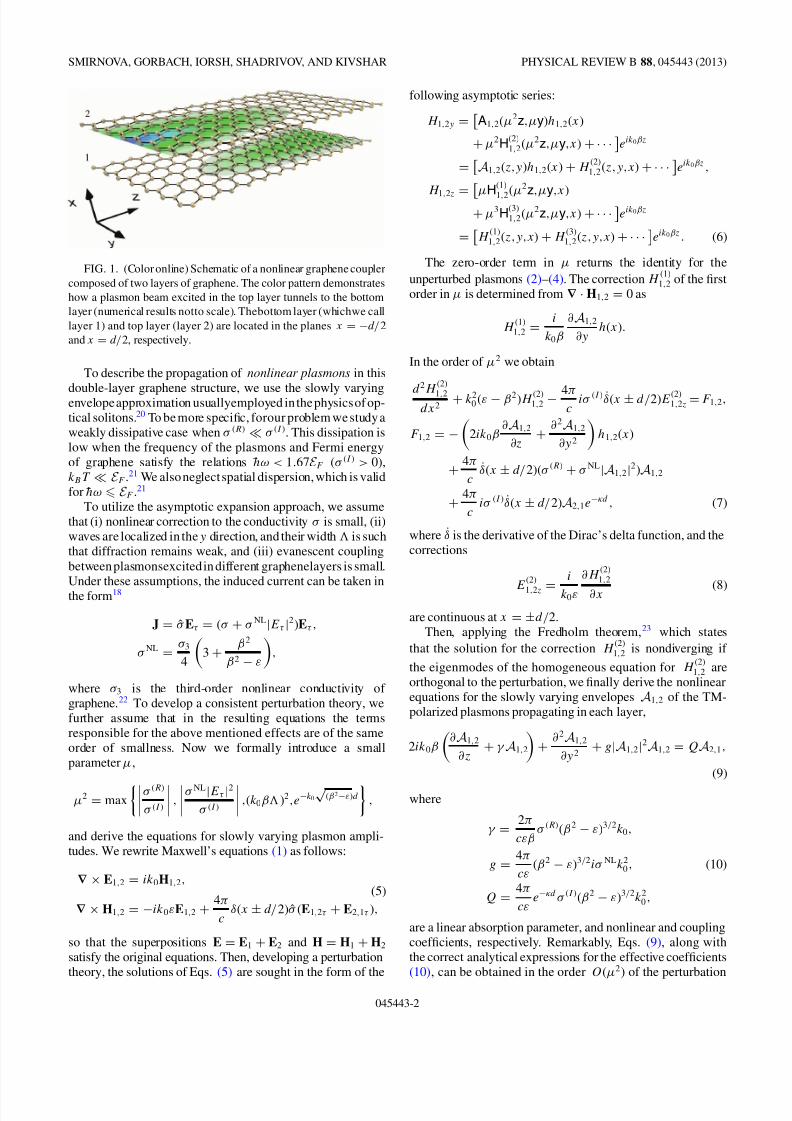
FIG. 1. (Color online) Schematic of a nonlinear graphene coupler

composed of two layers of graphene. The color pattern demonstrates

how a plasmon beam excited in the top layer tunnels to the bottom

layer (numerical results notto scale). Thebottom layer (whichwe call

layer 1) and top layer (layer 2) are located in the planes  x = −d/2

and x = d/2, respectively.

To describe the propagation of  nonlinear plasmons in this

double-layer graphene structure, we use the slowly varyingenvelopeapproximation usuallyemployed in the physics of op-

tical solitons.20 To be more specific, forour problem we study a

weakly dissipative case when σ (R) σ (I ). This dissipation is

low when the frequency of the plasmons and Fermi energy

of graphene satisfy the relations hω <  1.67E F    (σ (I ) > 0),

kB T   E F .21 We also neglect spatial dispersion, which is valid

for hω E F .21

To utilize the asymptotic expansion approach, we assume

that (i) nonlinear correction to the conductivity σ  is small, (ii)

waves are localized in the y direction, and their width is such

that diffraction remains weak, and (iii) evanescent coupling

between plasmonsexcited in different graphenelayers is small.

Under these assumptions, the induced current can be taken in

the form18

J =  σ Eτ  = (σ  + σ NL|Eτ |2)Eτ ,

σ NL = σ 3

4

3+ β2

β2 − ε

,

where   σ 3   is the third-order nonlinear conductivity of 

graphene.22 To develop a consistent perturbation theory, we

further assume that in the resulting equations the terms

responsible for the above mentioned effects are of the same

order of smallness. Now we formally introduce a small

parameter µ,

µ2 = max

σ (R)

σ (I )

,

σ NL|Eτ |2σ (I )

,(k0β)2,e−k0√ (β2−ε)d 

,

and derive the equations for slowly varying plasmon ampli-

tudes. We rewrite Maxwell’s equations (1) as follows:

∇ × E1,2 = ik0H1,2,(5)

∇ × H1,2 = −ik0εE1,2 +4π

cδ(x ± d/2)σ (E1,2τ  + E2,1τ ),

so that the superpositions   E = E1 + E2   and   H = H1 + H2

satisfy the original equations. Then, developing a perturbation

theory, the solutions of Eqs.  (5) are sought in the form of the

following asymptotic series:

H 1,2y =A1,2(µ2z,µy)h1,2(x)

+µ2H(2)1,2(µ2z,µy,x) + · · ·

eik0βz

=A1,2(z,y)h1,2(x)+ H 

(2)1,2(z,y,x)+ · · ·

eik0 βz ,

H 1,2z = µH

(1)

1,2(µ

2

z,µy,x)+µ3H

(3)1,2(µ2z,µy,x) + · · ·

eik0βz

= H 

(1)1,2(z,y,x) + H 

(3)1,2(z,y,x)+ · · ·

eik0 βz .   (6)

The zero-order term in   µ   returns the identity for the

unperturbed plasmons (2)–(4). The correction H (1)

1,2  of the first

order in µ  is determined from ∇ · H1,2 = 0 as

H (1)

1,2 =i

k0β

∂A1,2

∂yh(x).

In the order of  µ2 we obtain

d 2

H 

(2)

1,2

dx2  + k2

0 (ε − β2)H (2)1,2 − 4π

ciσ (I )δ(x ± d/2)E(2)

1,2z =F 1,2,

F 1,2 = −

2ik0β∂A1,2

∂z+ ∂ 2A1,2

∂y 2

h1,2(x)

+ 4π

cδ(x ± d/2)(σ (R) + σ NL|A1,2|2)A1,2

+ 4π

ciσ (I )δ(x ± d/2)A2,1e−κd ,   (7)

where δ is the derivative of the Dirac’s delta function, and the

corrections

E

(2)

1,2z =i

k0ε

∂H (2)

1,2

∂x (8)

are continuous at x = ±d/2.

Then, applying the Fredholm theorem,23 which states

that the solution for the correction   H (2)1,2   is nondiverging if 

the eigenmodes of the homogeneous equation for   H (2)

1,2   are

orthogonal to the perturbation, we finally derive the nonlinear

equations for the slowly varying envelopes  A1,2  of the TM-

polarized plasmons propagating in each layer,

2ik0β

∂A1,2

∂z+ γ A1,2

+ ∂ 2A1,2

∂y 2  + g|A1,2|2A1,2 = QA2,1,

(9)

where

γ  = 2π

cεβσ (R)(β2 − ε)3/2k0,

g = 4π

cε(β2 − ε)3/2iσ NLk2

0 ,   (10)

Q = 4π

cεe−κd σ (I )(β2 − ε)3/2k2

0 ,

are a linear absorption parameter, and nonlinear and coupling

coefficients, respectively. Remarkably, Eqs.   (9),  along with

the correct analytical expressions for the effective coefficients

(10), can be obtained in the order  O(µ2) of the perturbation

045443-2

7/27/2019 Graphene Coupler

http://slidepdf.com/reader/full/graphene-coupler 3/5

NONLINEAR SWITCHING WITH A GRAPHENE COUPLER PHYSICAL REVIEW B 88, 045443 (2013)

expansion by using the substitution

k0β = k0β +−i

∂

∂z− 1

2k0β

∂ 2

∂y 2

+ · · ·

in the modified dispersion relation (4), which in the presence

of the second layer takes the form

2ε

k0

 β2 − ε

= 4π

ω

σ (I ) − i

σ (R) + σ NL|A1|2

+ iσ (I )e−κd  A2

A1

+ · · ·

.   (11)

III. NONLINEAR SWITCHING

In the framework of the nonlinear amplitude equations

(9) disregarding losses and beam diffraction, we can analyze

different types of TM-polarized eigenmodes of a nonlinear

double-layer graphene waveguide. For further calculations,

we employ the following expressions for the grapheneconductivity:10,18,22

σ  = ie2

πh

  1

+ iνintra

+ 1

4ln

2−

2+

,   (12a)

σ 3 = −i3

32

e2

πh

(eV F )2h2

E 4F 3

  ,   (12b)

where = hω/E F , νintra = h/(E F τ intra), forthe doping level of E F  = 0.1 eV, = 1 (λ = 2π/ k0 ≈ 12.4 µm), τ intra = 10 ps,24

the Fermi velocity in graphene  V F  ≈ c/300,  ε = 4, and take

the separation between the layers as d  = 28 nm. We take quite

a large relaxation time and discuss the implications of this

choice below.We find that three types of nonlinear modes  can propagate

in this double-layer graphene coupler, namely, a symmetric (S)

mode with A1 = A2, an antisymmetric (AS) mode with  A1 =−A2, and an asymmetric (A) mode with  A1 = A2, similar to

the case of a nonlinear dimer.25 These modes are presented

in Fig.   2   through their (a), (b) transverse profiles and (c)

power-dependent shift of the nonlinear propagation constant.

In the linear regime, only symmetric (S) and antisymmetric

(AS) modes exist. However, above a critical power level, a

symmetry breaking occurs in this nonlinear system when a

different, asymmetric branch (A) emerges, and it describes

the nonlinear states where the power is not distributed equally

between the lower and upper graphene layers. The asymmetric

mode bifurcates at the point “p” from the antisymmetric

branch, and it is stable, being characterized by a predominant

energy concentration in the vicinity of one of the layers. The

AS mode becomes unstable above the critical power.

Next, we focus our attention on the power-controlled

switching of plasmon beams between the layers and study nu-

merically the propagation of a sech-like input beam launched

into the upper layer (as shown in Fig.  1). The input beam is

selected to be the fundamental solution of a single (uncoupled)

nonlinear equation, and it describes a spatial soliton.19 For

a peak power density of 6 W/m, the soliton beam width is

about 50 nm. This significant subwavelength localization is

supported by the large Kerr nonlinearity of graphene.18,19

0 2 4 6

0

5

10

Guided Power Density (W/m)

   k   0

      ∆       β   (     µ  m

  −   1   )

AS

S

A

p

(c)

−14 14

A

(b)

x (nm)

−14 14−2

1

0

1

2

AS

S

   E  z

   (  a .  u .   )

(a)

x (nm)

FIG. 2. (Color online) (a), (b) Examples of the transverse mode

profiles for symmetric (S), antisymmetric (AS), and asymmetric (A)

modes propagating in the double-layer graphene shown for the   Ez

component. (c) Shift of the nonlinear propagation constant vs the

mode power density in the guided plasmon mode propagating in the

z direction. Solid and dashed lines correspond to stable and unstable

branches, respectively.

In Fig. 3, we compare the corresponding switching charac-

teristics of the nonlinear graphene coupler for the continuous

plasmons (whose amplitude is constant along   y) (dashed

curve) and for the beams of a finite extent including the solitonswitching (solid curves). The coupler length is selected at the

half-beat length  L = π/(2Q), when in the linear regime the

input power transfers completely into the second layer.20 Apart

from an increase of the threshold power density, two regimes

of the coupler operation can be clearly distinguished.

0 2.5 5 7.5 100

0.2

0.4

0.6

Input Peak Power Density (W/m)

   T  r  a  n  s  m   i  s  s   i  o  n

L

N

FIG. 3. (Color online) Switching characteristics of the nonlinear

graphene coupler. Shown is a fraction of the power transmitted in the

pumped layer for a cw (dashed curve) and soliton input beam (solid

curve) in a half-beat-length coupler as a function of the input peak 

power density. Dashed-dotted curve: Calculated relative fractional

output power emergingfrom theother layer in the continuous plasmon

regime.

045443-3

7/27/2019 Graphene Coupler

http://slidepdf.com/reader/full/graphene-coupler 4/5

7/27/2019 Graphene Coupler

http://slidepdf.com/reader/full/graphene-coupler 5/5

NONLINEAR SWITCHING WITH A GRAPHENE COUPLER PHYSICAL REVIEW B 88, 045443 (2013)

8J. Chen, M. Badioli, P. Alonso-Gonzalez, S. Thongrattanasiri,

F. Huth, J. Osmond, M. Spasenovic, A. Centeno, A. Pesquera,

P. Godignon, A. Z. Elorza, N. Camara, F. J. Garcıa de Abajo,

R. Hillenbrand, and F. H. L. Koppens,  Nature (London)  487, 77

(2012).9N. I. Zheludev and Yu. S. Kivshar,  Nat. Mater. 11, 917 (2012).

10S. A. Mikhailov andK. Ziegler, Phys. Rev. Lett. 99, 016803 (2007).

11A. Vakil and N. Engheta,  Science 332, 1291 (2011).12L. Ju, B. Geng, J. Horng, C.Girit, M.Martin, Z. Hao, H.A. Bechtel,

X. Liang, A. Zett, Y. R. Shen, and F. Wang,  Nat. Nanotechnol.  6,

630 (2011).13S. H. Lee, M. Choi, T. Kim, S. Lee, M. Liu, X. Yin, H. K. Choi,

S. S. Lee, C. G. Choi, S. Choi, X. Zhang, and B. Min,  Nat. Mater.

11, 936 (2012).14I. V. Iorsh, I. S. Mukhin, I. V. Shadrivov, P. A. Belov, and Yu. S.

Kivshar, Phys. Rev. B 87, 075416 (2013).15S. A. Mikhailov, Europhys. Lett. 79, 27002 (2007).16K. L. Ishikawa, Phys. Rev. B 82, 201402 (2010).17E. Hendry, P. J. Hale, J. Moger, A. K. Savchenko, and S. A.

Mikhailov, Phys. Rev. Lett. 105, 097401 (2010).

18A. V. Gorbach, Phys. Rev. A 87, 013830 (2013).19M. L. Nesterov, J. Bravo-Abad, A. Yu. Nikitin, F. J. Garcia-Vidal,

and L. Martin-Moreno, Laser Photonics Rev. 7, L7 (2013).20Yu. S. Kivshar and G. A. Agrawal,  Optical Solitons: From Fibers

to Photonic Crystals (Academic, San Diego, 2003).21L. A. Falkovsky and A. A. Varlamov,  Eur. Phys. J. B   56, 281

(2007).

22S. A. Mikhailov and K. Ziegler,   J. Phys.: Condens. Matter   20,

384204 (2008).23G. A. Korn and T. M. Korn, Mathematical Handbook for Scientists

and Engineers (McGraw-Hill, New York, 1961).24T. Otsuji, S. A. Boubanga Tombet, A. Satou, H. Fukidome,

M. Suemitsu, E. Sano, V. Popov, M. Ryzhii, and V. Ryzhii,

J. Phys. D: Appl. Phys. 45, 303001 (2012).25J. C. Eilbeck, P. S. Lomdahl, and A. C. Scott,  Physica D  16, 318

(1985).26M. Currie, J. D. Caldwell, F. J. Bezares, J. Robinson, T. Anderson,

H. Chun, and M. Tadjerb, Appl. Phys. Lett. 99, 211909 (2011).27P. Neugebauer, M. Orlita, C. Faugeras, A.-L. Barra, and

M. Potemski, Phys. Rev. Lett. 103, 136403 (2009).

045443-5