i

GEOLOGICAL AND STRUCTURAL

INTERPRETATION OF PART OF THE BUEM

FORMATION, GHANA, USING

AEROGEOPHYSICAL DATA

By

Kenny Mensah Graham

(BSc Mathematic and Statistics)

A Thesis Submitted to the Department of Physics,

Kwame Nkrumah University of Science and Technology, Kumsai

in partial fulfillment of the requirements for the degree

of

MASTER OF SCIENCE (GEOPHYSICS)

College of Science

Supervisor: Dr. Kwasi Preko

April, 2013

ii

Declaration

I hereby declare that this submission is my own work towards the award of MSc

Geophysics degree and that, to the best of my knowledge, it contains no material previously

published by another person or material which has been accepted for the award of any other

degree of the University, except where due acknowledgement has been made in the text.

................................................... ................................... ............................

Student‘s Name Signature Date

Certified by:

................................................... ................................... ............................

Supervisor‘s Name Signature Date

Certified by:

................................................... ................................... ............................

Head of Dept.‘s Name Signature Date

i

Abstract

Airborne magnetic and radiometric datasets were processed to interpret the geology of part

of the Buem formation and estimate the depth to basement of magnetic source in the area.

The study was aimed at mapping lithology, delineating structural lineaments and their trends

as well as estimating the depth to magnetic source bodies of the area. The data processing

steps involved enhancement filters such as reduction to the pole, analytic signal and first

vertical derivative, Tilt angle derivative and these helped delineate geological structures and

lithology within the Buem formation. The radiometric datasets displaying the geochemical

information on potassium, thorium and uranium concentrations within the study area proved

valuable in delineating the Buem shales, sandstones, basalts and part of the Voltaian

sediments that underlie the Buem formation. Lineament analysis using the rose diagram

showed that the area is dominated by north-south (NS) and east-west (EW) trending

lineaments. Depths to the magnetic source bodies were estimated using Werner

deconvolution method, indicating two depth source models. The depth of the magnetic body

produced from the dike model ranged from 101.15 m to 1866.34 m and that of the contact

model ranged from 100.36 m to 983.709 m.

ii

Table of Content

Abstract ..................................................................................................................................... i

Table of Content ...................................................................................................................... ii

List of Figures ......................................................................................................................... vi

List of Tables ........................................................................................................................ viii

List of Symbols and Acronyms............................................................................................. viii

Acknowledgments................................................................................................................... ix

CHAPTER ONE .................................................................................................................... 1

1 INTRODUCTION ........................................................................................................... 1

1.1 Literature Review..................................................................................................... 2

1.2 Problem Definition................................................................................................... 6

1.3 The study area .......................................................................................................... 7

1.3.1 Background .......................................................................................................... 7

1.3.2 Location and Accessibility ................................................................................... 8

1.3.3 Climate ............................................................................................................... 10

1.3.4 Vegetation .......................................................................................................... 10

1.3.5 Relief .................................................................................................................. 11

1.4 Objectives of the Research ..................................................................................... 11

1.4.1 Justification of the Objectives ............................................................................ 12

1.5 Structure of the Thesis ........................................................................................... 13

iii

CHAPTER TWO ................................................................................................................. 15

2 Geological Background ................................................................................................. 15

2.1 Regional Geological Setting .................................................................................. 15

2.1.1 Proterozoic Birimian Supergroup ...................................................................... 16

2.1.2 The Tarkwaian System ...................................................................................... 21

2.1.3 Voltaian Basin .................................................................................................... 21

2.1.4 The Togo Series ................................................................................................. 23

2.1.5 The Buem Formation ......................................................................................... 24

2.1.6 The Dahomeyan ................................................................................................. 25

2.2 Geology of the Study Area .................................................................................... 26

2.2.1 Volcanic Group .................................................................................................. 27

2.2.2 Arenaceous Group ............................................................................................. 29

2.2.3 Argillaceous Group ............................................................................................ 30

2.2.4 Geological Structures in the Study Area ............................................................ 31

CHAPTER THREE ............................................................................................................. 33

3 THEORETICAL BACKGROUND ............................................................................... 33

3.1 Magnetism.............................................................................................................. 33

3.1.1 The Earth Magnetic Field .................................................................................. 34

3.1.2 The Geomagnetic Field ...................................................................................... 34

3.1.3 The International Geomagnetic Reference Field (IGRF) .................................. 38

3.1.4 Magnetic Susceptibility ..................................................................................... 39

3.1.5 Magnetism of Rocks and Minerals .................................................................... 40

iv

3.1.6 Aeromagnetic Survey......................................................................................... 42

3.1.7 Data Enhancement Techniques .......................................................................... 43

3.2 Radiometric ............................................................................................................ 49

3.2.1 Basic Radioactivity ............................................................................................ 50

3.2.2 Geochemistry of the Radioelements (K, U &Th) .............................................. 51

3.2.3 Disequilibrium ................................................................................................... 52

3.2.4 The radioactivity decay law ............................................................................... 53

3.2.5 Measurement of Gamma Radiation ................................................................... 55

3.2.6 Display of Radiometric data .............................................................................. 56

CHAPTER FOUR ................................................................................................................ 58

4 MATERIALS AND METHODS ................................................................................... 58

4.1 Data Acquisition .................................................................................................... 58

4.2 Data Processing ...................................................................................................... 59

4.2.1 Gridding ............................................................................................................. 59

4.2.2 Enhancement of Aeromagnetic Dataset ............................................................. 60

4.2.3 Depth to Basement ............................................................................................. 63

4.2.4 Airborne Radiometric Data ................................................................................ 64

CHAPTER FIVE ................................................................................................................. 67

5 RESULTS AND DISCUSSION .................................................................................... 67

5.1 Digitized Elevation Map (DEM) ........................................................................... 67

5.2 Magnetic ................................................................................................................ 69

5.2.1 Residual Magnetic Intensity, RMI ..................................................................... 69

v

5.2.2 Reduction to the Pole, (RTP) ............................................................................. 72

5.2.3 Analytical Signal ................................................................................................ 76

5.2.4 First Vertical Derivative (1VD) ......................................................................... 79

5.2.5 Upward continuation .......................................................................................... 80

5.2.6 Tilt derivative ..................................................................................................... 83

5.2.7 Summary ............................................................................................................ 86

5.3 Radiometric Data ................................................................................................... 91

5.3.1 Potassium ........................................................................................................... 92

5.3.2 Thorium.............................................................................................................. 95

5.3.3 Uranium ............................................................................................................. 97

5.3.4 Ternary map ....................................................................................................... 99

5.3.5 Summary .......................................................................................................... 102

5.4 Proposed Geological map .................................................................................... 104

5.5 Quantitative interpretation ................................................................................... 105

CHAPTER SIX .................................................................................................................. 110

6 CONCLUSION AND RECOMMENDATIONS ........................................................ 110

6.1 Conclusion ........................................................................................................... 110

6.2 Recommendations ................................................................................................ 112

References ............................................................................................................................ 113

Appendix .............................................................................................................................. 122

Appendix A 1 Generation of Werner deconvolution solutions ...................................... 122

Appendix A.2 Werner deconvolution solutions ............................................................... 123

vi

Appendix A.3 Script for extracting azimuth of lineaments ............................................. 123

List of Figures

Figure 1.1 Map of the Study area ............................................................................................. 9

Figure 2.1Generalised distribution of Birimian supracrustal belts in West Africa ............... 17

Figure 2.2 Geological map of Ghana showing study area ..................................................... 18

Figure 2.3 Geology map of Study Area ................................................................................. 29

Figure 3.1 Elements of Earth‘s Magnetic Field; Z: Vertical component H: Horizontal

component .............................................................................................................................. 35

Figure 3.2: The solar wind distorts the outer reaches of the earth‘s magnetic field causing

current loops in the ionosphere .............................................................................................. 37

Figure 3.3 A natural gamma-ray spectrum. (Vertical scale (numbers of counts) is

logarithmic) ............................................................................................................................ 56

Figure 5.1 Digital Elevation Map of the area ........................................................................ 68

Figure 5.2 Residual Magnetic Intensity, RMI grid map. ....................................................... 71

Figure 5.3 Reduction to the pole (RTP) image using an inclination of -11.1 and declination

of -4.9o.................................................................................................................................... 73

Figure 5.4 RTP drape over DEM viewed in 3D (Red - high magnetic signature and blue-

low magnetic signature) ......................................................................................................... 75

Figure 5.5 Analytic signal image of residual magnetic intensity........................................... 77

Figure 5.6 Analytical signal image draped over DEM viewed in 3D .................................... 78

Figure 5.7 First vertical derivative map of the RTP grid. (a) colour shaded map (b) grey

shaded map............................................................................................................................. 79

Figure 5.8 (b-d) RTP (grid) been continued upward to 100 m and 400 m and 800 m (a) RTP

image ...................................................................................................................................... 83

vii

Figure 5.9 Till angle derivative, TDR (a) TDR derived from RTP image displaced in grey

scale (b) TDR derived from RMI........................................................................................... 84

Figure 5.10 Interpreted fault, folds and contacts superimposed on the TDR image ............. 87

Figure 5.11 Interpreted structural map from the aeromagnetic dataset ................................. 88

Figure 5.12 Rose diagram showing the lineaments orientation of the study area ................. 89

Figure 5.13 Interpreted lithological map from aeromagnetic dataset .................................... 91

Figure 5.14 Gamma spectrometric image for Potassium (K) concentration ......................... 94

Figure 5.15 Gamma spectrometric image for thorium (eTh) concentration .......................... 96

Figure 5.16 Gamma spectrometric image for Uranium (eU) concentration .......................... 98

Figure 5.17 Ternary map of Study area (RGB=KThU) ....................................................... 100

Figure 5.18 Ternary image draped over DEM and viewed in 3D ....................................... 101

Figure 5.19 Interpreted lithological map from the radiometric dataset ............................... 103

Figure 5.20 Proposed Geological map of the study area ..................................................... 104

Figure 5.21 Profiles lines A-A1, B-B1 and C-C1 displayed on analytical signal image ....... 106

Figure 5.22 Werner deconvolution solutions from a magnetic profile A-A1 over the study

area: (a) residual magnetic intensity profile [nT], (b) depth [m], (c) susceptibility contrast

[SI]. (d) A simplified geological section of the interpreted geological map ....................... 107

Figure 5.23 Werner deconvolution solutions from a magnetic profile B-B1 over the study

area: (a) residual magnetic intensity profile [nT], (b) depth [m], (c) susceptibility contrast

[SI]. (d) A simplified geological section of the interpreted geological map ....................... 108

Figure 5.24 Werner deconvolution solutions from a magnetic profile C-C1 over the study

area: (a) residual magnetic intensity profile [nT], (b) depth [m], (c) susceptibility contrast

[SI]. (d) A simplified geological section of the interpreted geological map. ...................... 109

viii

List of Tables

Table 2.1 Classification of the Dahomeyan Stratigraphy ...................................................... 26

List of Symbols and Acronyms

eU Equivalent Uranium

eTh Equivalent Thorium

K Potassium

RTP Reduction to the pole

RMI Residual magnetic intensity

TDR Tilt angle derivative

1VD First vertical derivative

DEM Digital elevation map

UP Upward continuation

K Magnetic susceptibility

WGS84 World Geodetic System 1984

UTM Universal Transverse Mercator

ix

Acknowledgments

My first and foremost appreciation goes to the Almighty God for His unending strength,

mercies and grace towards me throughout the duration of this work. I sincerely thank my

supervisor Dr. Kwasi Preko for his motivation, encouragement, criticism and fatherly love

he showed me. I am highly indebted to my co-supervisor Mr. D. D. Wemegah for the

advice, motivation and the training he gave me on the GIS and the other geophysical

softwares. This work would not have been possible without the supports of Mr. Attah

(Ghana Geological Survey Department) who gave me the Oasis Montaj (Geosoft) training

and some advice. I am also grateful to the administration of Geological Survey Department,

Accra, for granting the dataset and allowing me to use their library for this work. I also

thank all the staff and MSc students of Physics Department for their immense support.

Finally to my family and all my love ones God bless you all.

1

CHAPTER ONE

1 INTRODUCTION

Airborne geophysics is a powerful technique available to the Earth scientists for

investigating very large areas rapidly. The broad view of the Earth that the airborne

geophysics perspective provides has been well recognized since the early days of balloon

photography and military reconnaissance (Dobrin and Savit, 1988). Compared with

ground-based methods, the advantages of these methods are that very large areas and

difficult terrain can be surveyed remotely in short periods of time thus making it very cost

effective. There are many airborne geophysical methods (e.g. gravity, radiometry,

magnetic, electromagnetic) whose operations are based on different physical principles,

techniques and physical properties (e.g. density, magnetic susceptibility, electrical,

conductivity, radioactive) of the Earth which can be employed for the provision of

solutions for various geological problems and structural mapping of an area. These

physical properties and formation of different rock types driven by different physical and

chemical compositions of the Earth vary from one area to another (Roy, 1966).

Depending on the dominant physical properties of the different rock types, the

appropriate geophysical methods have the potential to aid identification of the geology as

well as mapping geological structures likely to have developed in a particular area

(Afenya, 1982).

Aeromagnetic survey is a common type of geophysical survey carried out using a

magnetometer aboard or towed behind an aircraft allowing much larger areas of the

Earth's surface to be covered quickly. The resulting magnetic map shows the spatial

2

distribution and relative abundance of magnetic minerals (most commonly magnetite) in

the upper levels of the crust. The magnetic map allows a visualization of the geology and

geological structures of the upper crust of the Earth. This is particularly helpful where

bedrock is obscured by surface sand, soil or water. The apparent variation in the intensity

of the magnetic value (high, ridges and valleys) observed on the interpreted data are

referred to as magnetic anomalies for which a mathematical modelling can be used to

infer the shape, depth and properties of the rock bodies responsible for these anomalies

(Koulomzine et al., 1970).

Airborne radiometric data on the other hand is normally collected over large areas using

an aircraft mounted scanner with the data collected digitally. The scanner measures the

amount of potassium (K), thorium (Th) and uranium (U) radiation emitted from the

ground within certain parts of the electromagnetic spectrum. These three radioisotopes are

naturally found in most rock types. When the rock weathers, the relative proportions of

the potassium, thorium and uranium are reflected in the soils (Shi and Butt 2004).Many

times, there is a good correlation between patterns in the radiometric data and un-

weathered rocks (Gunn et al. 1997b). In 1961, Fugro Airborne Surveys estimated that 90

% of gamma rays are sourced from the top 30 – 45 cm of the soil. The amount and

proportion of K, Th and U which is emitted from the surface can be useful in mapping

soil properties and regolith (Gunn et al., 1997b).

1.1 Literature Review

Airborne geophysical surveys have been carried out in Ghana since 1952 (Kesse, 1985).

However, it was only within these few decades that airborne geophysical dataset was

3

established as a powerful tool in geological mapping (Reeves et al., 1997). On regional

scale, airborne geophysical data have often been used to identify several features, such as:

limits of geologic provinces, fold belts, sedimentary basin and tectonic and structural

detail of shear zones and overprinted structural trends (Direen et al., 2001).

In 2012, Cardero Ghana contracted Geotech Airborne Limited to conduct a 3,000 km line

of V-TEM, Magnetic, and Radiometric airborne geophysical survey to define the extent

of banded iron formation and outline and interpret the geological setting of the Shiene

area within the Buem Formation (PGEO, 2012). Delor, et al., (2009) used aeromagnetic

dataset to map structures such as fault, linearment, folds and share zones in the Nkwanta

area of Ghana. Delor, et al., (2009) also used airborne radiometric dataset to map

lithology from the ternary image of Potassium, Uranium and Thorium and also used the

Potasium grid to map out weathered zones. Various geophyiscal surveys have also been

conducted in various parts of the country mainly for the exploration of precious mineral

mainly gold by some mining comapies and the Geological Survey of Ghana. Some were

also carried out for the purpose of of scientific research.

In 1997, a high-resolution airborne geophysical survey over the Lake Bosumtwi impact

structure, Ghana, was carried out by the Geological Survey of Finland in collaboration

with the University of Vienna, Austria, and the Geological Survey Department of Ghana.

The magnetic data yielded a new model of the structure by showing several magnetic

rims and by providing hints for the existence of a central uplift. The gamma radiation data

turned out to be surprisingly valuable and clearly pinpoint two ring features (Pesonen, et

al., 2003).

4

Most of the airborne geophysical exploration works being carried out by mining

companies in Ghana are located along the well-known 'Ashanti belt', which hosts the

major economic deposit of the gold.

A complementary interpretation of magnetic data together with gravity, gamma-ray or

seismic dataset has shown to be very useful in geological and structural mapping

(Chandler, 1990; Gunn, 1997a). Asadi and Hale (1999) used the analytical signal of total

magnetic intensities to delineate intermediate composition magmatic rocks in the Takab

area of Iran. Chandler (1990) used the second vertical derivative enhanced-aeromagnetic

data together with gravity data to interpret the geology of the poorly exposed central part

of the Duluth Complex. Isolated outcrops and the well mapped surrounding areas were

used as geological controls. Gunn et al. (1997a) reported that correlation with seismic

reflection data has shown that geological structures mapped by magnetic data in

sedimentary rocks in northern Australia are indeed present. Experience from Finland also

show high degree of correlations between results from aeromagnetic data and bedrock

structure (Airo, 2005). Kesse (1985) reported that results from the 1960 magnetic survey

by Hunting Survey Limited across the Ashanti belt were quite satisfactory. Geological

interpretation based mostly on the magnetic maps proved successful in differentiating

lithologies, faults and fracture zones.

Silva et al., (2003) concentrated on processing and enhancing of airborne geophysical

data for accurate positioning of geological boundaries. The rationale was that in

exploration, we should not be looking for geophysical anomalies, but the responses

related to mineralization, lithology, and structure that may have economic importance.

Silva et al., (2003) also showed that aeromagnetic survey can be used to identify magnetic

5

greenstone units; important structures related to mineralization and allowed a better

understanding of structural geophysical pattern. The radiometric data is an excellent tool

for mapping and tracing individual lithological units in areas of less geological outcrop.

The most important host rocks or mineralized domains show high conductivity response

illustrating the utility of the airborne EM data as a tool to improve the geological mapping

(Silva et al., 2003).

The interpretation of the aeromagnetic survey over the Faiyum area, Western Desert,

Egypt was carried out by El-awady et al., (1984). Qualitative as well as quantitative

interpretations of the aeromagnetic data were carried out to obtain more information

about the crystalline basement structure and the local structure in the sedimentary section.

The analysis of the constructed magnetic maps which include the total intensity map, the

vertical map, the regional map, the residual map, the second vertical derivative map and

the downward continuation maps serve as basis for revealing the structural pattern of the

basement complex, and the shallower structures.

Galbraith and Saunders (1983) having analysed large amounts of airborne gamma ray

spectral data collected by the United States National Uranium Resource Evaluation

Program established that lithological unit can be classified according to the relationship

between Th and K. They have also shown that a classification based on a plot of log10Th

versus K can subdivide igneous rocks into conventional groupings. Gamma-ray data from

Lady Loretta in Australia were useful as a means of defining lithological changes within

formation which provided insight into regional variations in sediment maturity,

provenance and carbonaceous content (Duffett, 1998). Guillemont (1987), applying

gamma-ray spectrometry in Gabon, showed that it is possible to collect consistent data in

6

an equatorial environment, although such areas are characterised by dense vegetative

cover, substantial humidity and superficial alteration. He observed that the ternary colour

synthesis of K-U-Th concentration is a powerful tool for discriminating lithologies. In

Malawi, a ternary map compilation of spectrometric data in conjunction with an

interpretation of the accompanying magnetic data have provided the basis for the revision

of existing geological maps (Misener, 1987).

Billings (1998) and Wilford et al. (1997) reviewed the application of airborne gamma ray

spectrometry for regolith and soil mapping (since the interpretation of aerial photography

and satellite imagery has been the traditional means for the rapid mapping of soil types

over large areas) and found that the airborne gamma ray spectrometry interpretation is a

powerful means for regolith and soil mapping. Hardy (2004) on the other hand showed

that radiometric data are useful in identifying soil characteristics to the level of Australian

Soil Classification order and useful in delineating broad lithological units when used with

a geology map. Hardy (2004) also showed that the potassium and thorium data sets are

useful in delineating differences in the age of alluvium and broad difference in lithology

such as acid to basic igneous rock. Jones, (1990) performed a filed and geochemical

investigation of the Buem volcanic and its associate sedimentary rocks and showed the

various lithological unit and how they dip. Osae et al., (2006) also investigated the Buem

sandstone and determined their provenance and tectonic setting.

1.2 Problem Definition

Many airborne geophysical surveys have been conducted in Ghana including airborne

magnetic, gravity, electromagnetic and radiometric to identify the various geological

7

features over the country. The study area and its environs have been surveyed and studied

by several geoscientists, particularly for the surface geological mapping and geochemical

studies (Jones, 1990). The subsurface geological mapping has less been performed in the

study by integrating geological records and geophysical data. Irrespective of this, only a

little attempt has been made so far to understand the detailed relationship between

structural features observed on the ground and those extending into the subsurface.

This project is aimed at re-processing aeromagnetic and radiometric data to study major

surface and subsurface structures, and their relationship with surface structural features in

the study area. A new interpretation (detailed geological map) would be generated

showing magnetic units and structures, and the model of subsurface structures present in

the area of study. Attempt would be made to estimate the depth to basement of the

magnetic body.

1.3 The study area

1.3.1 Background

The study area is located mainly within the Jasikan District which is one of the old

districts in the Volta Region of the Republic of Ghana. It covers five (5) other districts in

the Volta region namely Hohoe, Kadjebi, Kpandu, Krachi and Biakoye (Fig. 1.1). The

area is situated about 260 km north-east of Accra, the capital of Ghana and 135 km from

Ho, the regional capital of Volta Region. It is one of the major agricultural production

areas in the Volta Region of Ghana. The area covers most of Buem Traditional Area.

Agriculture is the main source of employment and income generation venture for the

8

majority of the inhabitant in the area. Majority of the local population are farmers with

some involved GBG V VC VC VC VC in fishing, commerce and other works

(Dickson & Benneh, 1985). The perennial and annual water bodies in the area do support

much fishery activities, however big potentials exist for aquaculture in the area. The area

is connected to the national grid, with available infrastructure, financial institutions,

health and educational facilities. The road network in the area is relatively good (first and

second class roads). There are also lot of feeder roads that link some key farming

communities which are in deplorable state (Dickson & Benneh, 1985). The population of

the area is just over 66,000 (Ghana Statistical Service, 2012).

1.3.2 Location and Accessibility

The study area is located in the mid-east portion of the Volta Region of Ghana and the

area can be located between latitudes 7º 0‘ 18.0‖ N and 7º 40‘ 33.6‖ N longitudes 0º 8‘

45.6‖ E and 0º 30‘ 3.6‖ E. It is bounded on the North-East by Kadjebi and North-West by

Krachi District, on the west is the river Volta, Hohoe District to the South- East, and

Kpando District to the South-West. The area has a total land surface area of 2386.02 Km2

(Fig. 1.1)

9

Figure 1.1 Location map of the Study area

10

1.3.3 Climate

The area falls within the wet equatorial agro-climatic zone. The area experiences an

alternating wet and dry season each year. It experiences a double maxima rainfall regime.

The major rainy season occurs between May and July with the peak occurring in June

while the minor one occurs between September and October with the peak occurring in

October (Dickson & Benneh, 1985). The mean annual rainfall generally varies between

1250 mm and 1750 mm. The dry season is mostly between December and February. The

mean maximum temperature is 32ºc usually recorded in March whiles the mean minimum

temperature is 24 ºc usually recorded in August (Dickson & Benneh, 1985).

1.3.4 Vegetation

The vegetation is generally depicted by moist deciduous forest. Due to the relatively high

rainfall experienced annually in the eastern parts, the vegetation is thicker and more

luxuriant. The forests are made up of different species of trees typical of the semi

deciduous forest. The western part of the district is also characterized by the mixed

savannah dotted with tree vegetation. Bamboo and other wet species are also found,

especially along the banks of the streams and rivers. The vegetation supports wildlife and

major animals found are monkeys, antelopes, bush pigs, pangolins grass-cutter, and

reptiles. The area is endowed with the Odomi River Forest Reserve which covers about

18.45 km2

of land. The area is also noted for the cultivation of shallow-rooted crops such

as: pineapples, sugarcane, vegetables, maize and rice (Dickson & Benneh, 1985).

11

1.3.5 Relief

The topography of the area is hilly and undulating becoming almost flat in certain areas.

It is almost surrounded by mountain ranges, typically is the Buem-Togo Ranges which is

an extension of the Akuapem Ranges. The eastern parts of the area are relatively higher

with occasional heights ranging between 260 m – 800 m above sea level. The areas

consist of the western ridge which comprise of the Odumasi-Abutor range in the south,

the Akayoa-Abotoase range in the middle and the Tapa range in the north. The

characteristic features of the above hills are their approximate north to south trend, which

is sub-parallel to the regional foliation, and the general steeper western scarps with local

development of cliff faces (Dickson & Benneh, 1985).

1.4 Objectives of the Research

The main objective of the research is to carry out a comprehensive geological

interpretation of the study area using airborne geophysical data namely magnetic and

radiometric data.

Specific objectives are to:

Map the lithology of the study area.

Map geological structures of the study area.

Estimate the depth to basement of magnetic body in the area.

12

1.4.1 Justification of the Objectives

The continued expansion in the demand for minerals of all kinds since the turn of the

century have led to the development of many geophysical techniques of ever increasing

sensitivity for the detection and mapping of the unseen deposits and structures (Telford et

al., 1990). The structural control and the hydrothermal alteration of the rocks and

geophysical characterization of mineral deposits can be discerned from integrated

interpretation of airborne magnetic and radiometric data (Airo, 2002). In addition,

integrated geophysical method offers a quick way of examining large areas, and it should

prove useful in the search for mineral deposits in other parts of the world (Airo and

Loukola-Ruskeeniemi, 2003).

The Earth's magnetic field of an area is directly influenced by geological structures,

geological composition and magnetic minerals, most often due to changes in the

percentage of magnetite in the rock. Objects that are underground can warp the simple

patterns of the Earth's magnetic field into complex shapes (Grant and Martin, 1966). The

magnetic map allows a visualization of the geological structure of the upper crust of the

Earth, the presence of faults and folds (Atchuta and Badu, 1981). In exploration

geophysics, aeromagnetic maps are important tools for mapping geology (Smith and

O‘Connell, 2007). A study of these shapes on a magnetic map can reveal much

information about the features that are underground. This information can include the

location, size and shape, volume or mass, and depth of the features; in some cases, the age

of a feature and its material (stone, soil, metal) may be estimated (by logging) (Telford et

al., 1990).

13

Radioactive elements occur naturally in the crystals of particular minerals and it changes

across the Earth‘s surface with variations in rock and soil type (Gregory and Horwood,

1961). The energy of gamma rays is related to the source radioactive element, hence, it

can be used to measure the abundance of those elements in an area. Airborne radiometric

survey measures the natural radiation in the Earth‘s surface, which can give the

distribution of certain soils and rock type formation. Airborne radiometric survey is also

useful for the study of geomorphology and soils. The radiometric data is an excellent tool

for mapping and tracing individual lithological units in areas of outcrop (Beltrão et al.,

1991). Many times, there is a good correlation between patterns in the radiometric data

and un-weathered rocks (Gunn et al., 1997b).

1.5 Structure of the Thesis

The thesis work has six (6) chapters with each chapter addressing a main heading.

Chapter one introduces the subject matter, outlining the background of the research,

objectives of the research, justification of the objectives of the research, location and

accessibility of the research area, physiography, climate and occupation of inhabitants of

the research area as well as literature review.

Chapter two gives the general overview of the geological settings. It reviews both the

regional and local geology of the area.

Chapter three outlines the main fundamental theory behind airborne radiometric and

magnetic survey, taking into account some enhancement techniques applicable to

magnetic and radiometric data.

Chapter four gives an overview of the methods used to acquire the datasets and how the

enhancement techniques were used in enhancing the datasets. This chapter also outlines

the processing steps employed in the data processing.

14

Chapter five analyses the various maps obtained from the radiometric and magnetic

datasets. Interpretations to the deduced maps are also given in this chapter. Finally, this

chapter correlates the magnetic and radiometric data to produce an integrated geological

map of the study area.

Chapter six draws conclusions from the research and makes recommendations for future

work.

15

CHAPTER TWO

2 Geological Background

2.1 Regional Geological Setting

Most part of Ghana falls within the West African Shield (Fig. 2.1). The main rock units

underlying the country are the Birimian, the Tarkwaian, the Dahomeyan Systems, the

Togo Series and the Buem Formation. Intruded into the Birimian rocks are Cape Coast

and Winneba granitoids (basin type), Dixcove granitoids (belt type) and the rare Bongo

granitoids. These Precambrian rocks are overlain by the Voltaian System (Late

Proterozoic to Paleozoic) (Wright, 1985). Younger rocks as well as unconsolidated

sediments occur at various places along the coast (Fig. 2.2).

The geology of Ghana can be divided into three main geologic provinces (Hasting, 1982):

1) an early Proterozoic Birimian Supergroup and Tarkwaian group of the main West

African shield occupying the west and northern parts of the country;

2) a Pan African province covering the Dahomeyan, Togo and Buem formations in

the southeast and eastern parts of the country; and

3) Infracambrian/Palaeozoic sedimentary basin situated in the central and eastern

parts of the country Fig. 2.1.

16

2.1.1 Proterozoic Birimian Supergroup

The Birimian Supergroup in Ghana has long been divided into two series: (1) a lower

series of mainly sedimentary origin, and (2) an upper series of the greenstones, mainly

metamorphosed basic and intermediate lavas and pyroclastic rocks (Junner, 1935). The

lower Birimian rocks comprise an assemblage of fine-grained rocks with a large volcano

clastic component. Typical lithologies include tuff, aceous shale, phyllite, siltstone,

greywacke and some chemical (Mn-rich) sediment. The upper Birimian rocks comprise

mostly basalts with some interflow sediment (Eisenlohr and Hirdes, 1992). Recent

studies, however, shows that the lavas of the greenstone belts in Ghana and the sediments

of the sedimentary sequence in the basins were deposited contemporaneously as lateral

facies equivalents (Leube et al., 1990).

17

Figure 2.1Generalised distribution of Birimian supracrustal belts in West Africa (after

Wright et al., 1985)

18

Figure 2.2 Geological map of Ghana showing study area (modified after GSD (1988))

19

2.1.1.1 Birimian Metavolcanics

There are six volcanic belts in the Birimian, namely the Kibi-Winneba, Ashanti, Sefwi,

Bui, Bole-Navrongo and Lawra belts. The belts have a slight keel-shaped outline that is

perhaps produced by the associated diapiric, intrusive plutons (Kesse, 1985). The belts

consist mainly of metamorphosed basaltic and andesitic lavas, now hornblende- actinolite

schists, calcareous chlorite-schists and amphibolites (the greenstones). Minor intrusions

of mafic rocks cut the volcanics. Volcaniclastic sediments occur interbedded within the

basaltic flows of all volcanic belts (Leube et al., 1990). Metamorphism in most volcanic

rocks is confined to the chlorite zone of the greens schist facies. Amphibolite-facies

assemblages occur sporadically but especially along the margins of granitoid bodies.

2.1.1.2 Birimian Metasediments

Birimian metasedimentary rocks of Ghana are divided into: (1) volcaniclastic rocks; (2)

turbidite-related wackes; (3) argillitic rocks; and (4) chemical sediments. Boundaries

between these subdivisions are gradational (Leube et al., 1990). The volcaniclastic

sediments comprise chiefly of sand-to silt-sized, partly reworked pyroclastics that is

shown by the presence of quartz, idiomorphic plagioclase crystals, chloritised glass

fragments, and the absence of heavy minerals (Leube et al., 1990).

2.1.1.3 Birimian Granitoids

Four main types of granitoids are recognised in the Birimian of Ghana. They include

Winneba, Cape Coast, Dixcove and Bongo granitoids (Junner 1935; Kesse, 1985). The

latter three have been recently termed ―Basin‖, ―Belt‖ and ―K-rich‖ granitoids. (Leube et

20

al., 1990). The Cape Coast (Basin type) and Dixcove (Belt type) granitoids are

widespread in Ghana, the Winneba belt is limited to small areas near Winneba, and the

Bongo type crops out in the Bole Navrongo Belt and in the Banso area (Kesse, 1985).

The (Basin type) granitoids occur only within the Birimian sedimentary basins. Some of

them are two mica granites. This group also includes gneisses, and these are especially

well developed in the metasedimentary basin. They are typically biotite-bearing. It has

been suggested that the Basin granitoids, which appear migmatitic in some localities,

might represent an older continental basement on which the Birimian supracrustals were

deposited. Based on the degree of foliation, early workers assumed that the Basin type

granitoids intruded during regional deformation and that Dixcove granites were emplaced

after deformation (Kesse, 1985). However, later work by Hirdes et al. (1992)

demonstrated, in contrast to long held views that Dixcove granitoids formed at about

2,175 Ma and are about 60 and 90 Ma older than the Cape Coast granitoids. Taylor et al.

(1988) suggest that the Cape Coast and Dixcove granitoids are coeval.

Belt type granitoids are metaluminous and typically dioritic to granodioritic in

composition. They intrude Birimian volcanic rocks. They are typically hornblende-

bearing and are commonly associated with gold mineralisation where they occur as small

plutons within the volcanic belts. The granitoids are massive in outcrop, do not have a

compositional banding or foliation, and are thus generally considered post-deformation.

However, belt-type granitoids have never been shown to intrude or crosscut basin

granitoids (Murray, 1960). The granitoids commonly contain basalt xenoliths, and there

appears to be a gradational boundary between finer and coarser grained belt granitoids

and basalts (Hirst, 1946).

21

2.1.2 The Tarkwaian System

The Tarkwaian is a Proterozoic supracrustal system overlying the Birimian. It consists

mainly of shallow water sediments and is present in all the Birimian volcanic belts

(Junner, 1935). It consists of coarse clastic sedimentary rocks that include conglomerates,

arkoses, sandstones and minor amounts of shale. The Tarkwaian is usually regarded as

the detritus of Birimian rocks that were uplifted and eroded following the Eburnean tecto-

thermal event (Eisenlohr and Hirdes, 1992). Economically, the most important unit of the

Takwaian is the Banket series which contains economic concentrations of gold in several

areas.

2.1.3 Voltaian Basin

Almost one third of Ghana is covered by sediments of the inland Voltaian Basin which

covers an area of about 103,600 km2; it consists mainly of flat lying or very gently

dipping sediments sitting on a major Precambrian unconformity (Griffis, et al. 2002).

This unconformity marks an erosional surface, which apparently covered the entire Man

Shield. The Voltaian Basin area appears to have been the eastern margin of a large West

African cratonic block, which had broken away from the former supercontinent Rodinia

(Hoffman, 1999). This block would later join up with other cratonic blocks to form a new

supercontinent, Gondwana, during the Pan-African thermo tectonic event (approximately

600-550 Ma). The Voltaian Basin is a structural basin. Sedimentary rocks along the

eastern margin were folded during erogenic activity associated with a late Precambrian to

early Paleozoic thermal event, the Pan-African Thermo-Tectonic Episode (Kennedy,

1964).

22

Numerous geological studies have been carried out in the Voltaian Basin starting from the

early days of the former Gold Coast Geological Survey. Most of these covered only

restricted areas but, in 1946, Hirst provided a more comprehensive evaluation of the

stratigraphy on a regional basis and established an Upper, Middle and Lower series of

units. Shallow marine, quartz rich sediments and a basal conglomerate dominate the

Lower series. The very thick Middle series include a great variety of sandstones and

shales with some conglomerate interbeds, a few carbonate sequences and clastic units

generally identified as glacial tillites. The Upper series is more or less restricted to the

central and eastern parts of the basin and it is dominated by massive, quartz-rich

sandstones.

More detailed stratigraphical studies have revised the division of the Voltaian Basin

sediments modestly and attempted to better define the regional tectonic setting and

stratigraphic correlations (Kesse, 1985). The current stratigraphy includes the lower

Bombouaka Supergroup, which is approximately 1000 m thick and is dominated by

mature sandstones and a central section of siliceous and clay-rich units; these were

deposited on a shallow submerged epicontinental marine platform. The succeeding Oti (or

Penjari) Supergroup is considerably thicker (average is about 2500 m) and is

unconformable with the underlying Bombouaka sediments. The Oti sediments include a

distinctive lower sequence with tillite and sandstones, carbonate, and fine grained cherty

sediments (silexite). The Oti also includes thick sequences of less mature clastic

sediments indicative of a deeper marine depositional environment, probably on a passive

continental margin. In places, the tillites actually sit on Birimian basement and indicate

extensive local erosion and gouging by Neoproterozoic glaciers that probably correlate

with similar events in various other parts of Africa and most likely indicate a major,

23

worldwide glacial event (Hoffman, 1999). The youngest sequence of sediments in the

Voltaian Basin, are exposed only in Ghana and are referred to as the Tamale Super group

(Affaton et al., 1980). This sequence is only about 500 m thick and features a basal

section of sediments that also include glacial tillites. These are overlain mainly by cross-

bedded quartz sandstones with subordinate shale and mudstones that are now interpreted

to represent a foreland molassic basin (Affaton et al., 1980).

2.1.4 The Togo Series

The Togo Series is an irregular, fault-bounded belt of metamorphic units that comprise

the series of hills and ridges (Akwapim) that start from just west and north of Accra and

extend along the Ghana-Togo border and into northern Benin where it is called the

Atacora Range. The Togo Series consists mainly of metamorphosed sediments (quartzite,

schist, phyllite and marble) but there are some metavolcanics as well. Along major faults,

slices of higher grade metamorphic (Dahomeyan) and lenses of ultramafic and mafic units

can be found. The Togo Series originally consisted of alternating arenaceous and

argillaceous sediments, which were converted into phyllites, schists and quartzites in the

wake of metamorphism, except in few places, where unaltered shales and sandstones

occur. Quartzite, quartz-schist, sericite quartz schist, sericite schist and phyllite are the

predominant rocks, but hornstones, jaspers and hematite quartz-schists some of which

were formed after the deposition of the sediments also occur in the Togo Series (Junner,

1935). The levels of metamorphism and degree of deformation increase towards the

southeast (Wright et al., 1985). To the east of the Togo Series is a generally low-lying

area (Accra plains) underlain by high-grade, Dahomeyan metamorphic terrain. The level

of metamorphism is largely of amphibolite facies although there are areas of high-grade

24

granulite facies with garnet, pyroxene, and scapolite. The typical rock lithologies include

migmatites, gneisses, mica schists, amphibolites, marbles, syenites and granitoids. The

Togo Belt marks the western limits of a very large area affected by the Pan-African

thermo tectonic event that peaked at about 600-550 Ma and whose effects extend right

across Nigeria (Griffis, et al., 2002). The Togo Belt is now recognized to be a collisional

belt and suture zone between the West African Birimian craton and an eastern cratonic

block that became welded together at a time the supercontinent of Gondwana was being

created (Hoffman, 1999).

2.1.5 The Buem Formation

The westernmost Buem Formation consists of a thick, lower sequence of clastic

sediments with some carbonate and tillite units succeeded by clastics and volcanics that

include mafic flow units and pyroclastics (Kesse, 1985). The formation consists of a thick

sequence of shale, sandstone, and volcanic rocks with subordinate limestone, tillite, grit

and conglomerate (Dapaah-Siakwan and Gyau-Boakye, 2000). The rocks underlie an

elongated area on the eastern part of the country extending northeast to the Republic of

Togo. The sandstones overlie the basal beds of shale and the conglomerate and tillite

overlie the sandstone (Dapaah-Siakwan and Gyau-Boakye, 2000). Rocks of volcanic

origin form the upper part of the Buem formation and include lava, tuff, and agglomerate

interbedded with shale, limestone, and sandstone (Dapaah-Siakwan and Gyau-Boakye,

2000). Rocks of this formation are largely inherently impervious, but fracturing and

weathering create secondary permeability in them at some locations to form high yielding

aquifers. In general, the rocks of the Buem Formation are not metamorphosed, and

deformation is expressed as the result of thrust tectonics with development of imbricated

25

thrust systems and duplexes. Folds are not well developed but are expressed as chevron

folds in the finest grained material (Kesse, 1985). Folding and faulting also makes it

difficult to estimate average thicknesses for the various sequences but the volcanics and

closely related clastics are at least 5000 m thick and the underlying clastic sequences are

of the same order (Kesse, 1985). The deformation in the Buem Formation includes large-

scale thrusting towards the west. Closely associated with the thrust sheets are numerous

occurrences of serpentinized ultramafic bodies (Wright et al., 1985). Early workers in the

region generally considered the Buem Formation to be older than the Voltaian Basin

sediments (Kesse, 1985) but detailed studies by Affaton et al., (1980) indicate that the

Buem Formation is probably a lateral equivalent to the Oti Supergroup of the Voltaian

Basin. The mafic and ultramafic units probably represent tectonically emplaced slices of

paleo-oceanic crust caught up in the suturing of adjacent continental blocks during the

Pan-African orogeny (Griffis, et al., 2002).

2.1.6 The Dahomeyan

The Dahomeyan System is a part of the second major tectono-stratigraphic terrain in

Ghana; it underlies eastern and south-eastern Ghana. The Dahomeyan is the easternmost

rock group in Ghana and differs significantly from other rocks in Ghana in that it is

composed of high grade metamorphic rocks. The system consists of four lithologic belts

of granitic and mafic gneiss. The mafic gneisses are relatively uniform oligoclase,

andesine, hornblende, salite and garnet gneisses of igneous origin and generally of

tholeiitic composition (Holm, 1974). The granite gneisses interlayer with the mafic gneiss

and are believed to be metamorphosed volcaniclastic and sedimentary rocks. The

Dahomeyan System occurs as four alternate belts of acid and basic gneisses trending

26

SSW to NNE from the coastal plains extending into Togo (Kennedy, 1964). Mani (l978)

has suggested the following Dahomeyan stratigraphic scheme:

Table 2.1 Classification of the Dahomeyan Stratigraphy (Modified after Mani, 1978)

Acid Dahomeyan Pegmatite, aplite, quartz veins, Cape Coast granite,

granitic gneiss and migmatite, Granite, gneiss

Alkalic Gneiss Kpong conglomerate, nepheline gneiss

Basic Dahomeyan

Basic Intrusive Dolerite, norite, chromitiferous pyroxenite

Metabasics Garnet-hornblende-gneiss, garnet-hornblende-

(pyroxene)-gneiss, hornblende and biotite schist

Intruded in the Dahomeyan are granites, nephelinesyenite and dikes of various

compositions (Kennedy, 1964).

2.2 Geology of the Study Area

The study area is mainly dominated by the Buem Formation which defines the eastern

limit in Ghana of the Voltaian Basin. It consists mainly of a thick sequence of shale,

sandstone, and volcanic rocks. It also includes bedded cherts and siliceous shales

(silexites), limestones, dolomites and, north of Togo, some banded iron formation (BIF).

Volcanic formations, of alkaline to calc-alkaline affinity, are interbedded in the formation

(Delor, et al., 2009). In general, the rocks of the Buem Formation are not metamorphosed,

and deformation is expressed as the result of thrust tectonics with development of

imbricated thrust systems and duplexes. Folds are not well developed but are expressed as

chevron folds in the finest grained material. Close to their contact, the area is the folded

and metamorphosed with the Togo series and the Voltaian formation (Delor, et al., 2009).

27

It is acknowledged that infill material of the Buem was probably derived from the

Voltaian Basin and from the Togo Group (Delor, et al., 2009).

2.2.1 Volcanic Group

The volcanic group includes many closely intermingled volcanic rock types: various

facies of basalts, microgabbros, andesites or trachytes, and coarse-grained polymictic

pyroclastites or agglomerates (Geotech Airborne Limited, 2009). The volcanic group of

rock occurs along the western margin of the study area (Fig. 2.3). The rocks area better

exposed on the Abutor Hill Range southwest of Kwamekrom and in stream valleys

northwest and southwest of Odumasi (Blay, 2003). The volcanic rocks are poorly exposed

in the lowland area west of Tapa-Abotoase. West of Akayao and the hill range of which

Owisa is a peak, they are not exposed but their presence is indicated by characteristic dark

brown clayey nature of the soil and a few scattered fragments of basalt and andesite

(Blay, 2003). The Abutor-Odumasi Range is formed by hard resistant volcanic

agglomerate, vesicular basalt and pink jasper. Some of these east-west valleys are marked

by faults (Blay, 2003).

Two volcanic rock types occur in the area, namely, agglomerate and amygdaloidal basalt,

which exhibit pillow lava structure (Jones, 1990). Both types are so closely intermingled

that it is not possible to map them separately. The agglomerates vary in colour from pale-

green to dark greenish-grey and are hard and massive. These are also very coarse and

contain angular rock fragments of basalt, pink jasper and baked greenish shale. The

basaltic types are coloured greenish-black to greyish-black. They are massive, fine-

grained, and are cut by random calcite veinlets. Generally the basalts are vesicular in

28

texture (Blay, 2003). The sediments enclosing the volcanics are red shales, feldspathic to

quartz arenite sands, conglomerates, jasper and minor limestone (Jones, 1990). The Buem

volcanic rocks are mainly documented to the south of the Kpandu area. The

corresponding volcanic component of the Buem was described from bottom to top as

basalt pillow lavas, feldsparphyric basalts, olivine-phyric and aphyric basalts, rhyolitic

flows, agglomerates and tuffs (Delor, et al., 2009).

29

Figure 2.3 Geology map of Study Area (modified after GSD, 1988)

2.2.2 Arenaceous Group

The arenaceous rocks include medium-to coarse-grained feldspathic sandstones,

quartzitic sandstones, gritty quartzites, quartz-schist and poorly exposed conglomerate.

The conglomerate occurs mainly as boulders south of Tepa-Abotoase. Generally, the

arenaceouse rocks outcrop in the graphically higher ground (Blay, 2003). Minor thin band

of vary-coloured shales and siltstones occur interbedded with the sandstone. The gritty

quartzite and quartz-schist occur close to or within the Buem-Togo contact zone. Thin

argillites were found interbedded with the arenites (Blay, 2003).

The Buem sandstones in some parts of the area are poorly exposed. The best exposed in

those area are found in and around Tetaman and across the hill range of Borada where

they are interbedded with thin-bedded shale. Good exposures of coarse-grained pebbly,

haematitic, quartz-veined sandstone are also found along the southwest path from Sokpo

to Akpafu-Tadzi. There are also well exposed sandstones on the western ridge south of

Akayao. The path from Tapa-Amanya north-westwards to Tepa and Akaniem and from

Tapa to Odei also have comparatively good sandstone exposures. From Tapa westward to

either Odei or Akaniem, the sandstones become steadily coarse-grained until the foot of

the scarp face where coarse-grained and pebbly type outcrop (Blay, 2003). The

sandstones range from yellow-orange feldspathic sandstones to grey-white quartz arenites

with well-rounded and spheroidal quartz grains. The sandstones are frequently cut by

quartz veins (Jones, 1990).

30

In the west-central ridge area the sandstones are fairly well exposed except along the

Kabo Forest Hill. The Togo Plateau is formed by hard, massive, feldspathic and quartzitic

sandstone which can be traced geographically into the Nkonya and Alavanyo area to the

south of the study area. Bell (1962) mapped and referred to them as quartzites. The

sandstones form high cliffs on the scarp face. In Jasikan town, the sandstones are gritty,

rather schistose and are cut by small quartz veins. Identical types outcrop between Jasikan

and Tetaman along the main road. These sandstones are also deformed and brecciated.

They contain clayey and other rock fragment (Osae et al., 2006).

The Buem arenaceous rocks of the study area are poorly sorted sandstones consisting of

sub-angular and sub-rounded grains of quartz, albite, microcline, and in some cases shales

and phyllitic rock fragments. Towards the Togo boundary and at the foot of the hill

ranges, the sandstones are essentially quartzites. The Buem sandstones do not resemble

either the Voltaian sandstone or the Togo Series sandstones. The lenticular shape of the

sandstone bodies and paucity of sedimentary structures in the massive sandstones suggest

their deposited as alluvial fan deposits (Jones, 1990). Osae et al., (2006) classified Buem

sandstones as quartz arenite and feldspathic arenite. He said the feldspathic arenites is

generally composed of argillaceous materials and the quartz arenites are typically

cemented with quartz, hematite (Fe2O3), and sericite. He added that the quartz arenites are

depleted of K2O and TiO2 but enriched in Fe2O3 as compared to the feldspathic arenites.

2.2.3 Argillaceous Group

This argillaceous group are of massive shaly rock with interbedded siltstones, thin-bedded

sandstones and impure limestone members. The shales are reddish-brown with occasional

31

yellow or green bands showing bedding (Jones, 1990). Except places where minor shale

is found to be interbedded with the arenaceous Buem rocks. The Buem argillaceous rocks

are restricted to lower topographic level and in stream valleys where they are better

exposed (Blay, 2003).

In the area, the shale outcrops only in Nuboiasn Tsi streams west of the Helu-Soba motor

road. The shales exposed in the two streams are intensely minor folded and deformed and

may be termed metashales (Blay, 2003). In the Nsuta, Guaman and Atonko areas,

massive, deformed pale yellow, purple and greenish micaceous shales outcrop. The road

linking Odomi and Jasikan exposes quite a good section of the pinkish, greenish and pale

yellow shale. The greenish types are more micaceous and siliceous and show evidence of

having been tectonically deformed. The Papase massive shale is beautifully exposed at

Kwamekrom. Streams south of Papase are underlain by pale yellow and purple shales

with minor interbedded fine grained shaly sandstones (Blay, 2003). The only sedimentary

structures seen in the shales were dessication cracks and ripples west of Kwamikron

(Jones, 1990).

2.2.4 Geological Structures in the Study Area

The foliation of the rocks in the study area is parallel to the bedding. The rocks are

generally not metamorphosed except towards their boundary with the Togo and the

Voltaian. Reference to the geological map shows that, the strike and dip of the bedding

plane vary from place to place (Bell and Crook, 2003). Junner (1940) believed that the

sandstones of the Kpandu Hills and Dayi Plateau were strongly folded and showed

greater dips than the volcanics. The shape of the minor folds is essentially isoclinal. The

32

folding is interpreted to be represented by open to close asymmetric folds. Stereographic

analysis of the area revealed a north-northwest fold trend, with fold axes plunging at

south-southeast (Blay, 2003). Stereographic analysis of the area revealed the following

fault trend: north faults, north-northeast faults and south-east fault. The most important

ones are the north fault, which are recognised as thrust fault (Blay, 2003). The other faults

are essentially cross faults. They are mostly normal fault with, in some case, fairly large

strike slip movement as deduced from topographic displacement of north trending hill

(around the Alavanyo hills) (Blay 2003).

33

CHAPTER THREE

3 THEORETICAL BACKGROUND

3.1 Magnetism

The principle underlying the operation of the Magnetic Method is based on the fact that

when a ferrous material is placed within the Earth's magnetic field, it develops an induced

magnetic field. The induced field is superimposed on the Earth's field at that location

creating a magnetic anomaly. Detection depends on the amount of magnetic material

present and its distance from the sensor. The anomalies are normally presented as profiles

or as contour maps.

Ninety percent of the Earth's magnetic field looks like a magnetic field that would be

generated from a dipolar magnetic source located at the center of the Earth and aligned at

11.5o, with the Earth's rotational axis. The remaining 10 % of the magnetic field cannot be

explained in terms of simple dipolar sources. The main field (90 %) is the largest

component of the magnetic field and is believed to be caused by electrical currents in the

Earth's fluid outer core. For exploration work, this field acts as the inducing magnetic

field. Crustal magnetic field is the portion of the magnetic field associated with the

magnetism of crustal rocks. This portion of the field contains both, magnetism caused by

induction from the Earth's main magnetic field and from the remnant magnetization of

both surface and crustal rocks. Relatively small portion of the observed magnetic field is

generated from magnetic sources external to the earth. This field is believed to be

produced by interactions of the Earth's ionosphere with the solar wind.

34

3.1.1 The Earth Magnetic Field

From the point of view of geomagnetism, the earth may be considered as made up of

three parts: core, mantle and crust. Convection processes in the liquid part of the iron core

give rise to a dipolar geomagnetic field. The mantle plays little part in the earth's

magnetism, while interaction of the (past and present) geomagnetic field with the rocks of

the Earth's crust produces the magnetic anomalies. Magnetic field in SI units is defined in

terms of the flow of electric current needed in a coil to generate that field (Reeves et al.,

1997). As a consequence, units of measurement are volt-seconds per square metre or

Weber/m2 or Teslas (T). Since the magnitude of the earth's magnetic field is only about 5

x 10-5

T, a more convenient SI unit of measurement in geophysics is the nanoTesla (nT =

10-9

T). The geomagnetic field varies from less than 22000 nT in southern Brazil to over

70000 nT in Antarctica south of New Zealand. Magnetic anomalies as small as about 0.1

nT can be measured in conventional aeromagnetic surveys and may be of geological

significance. One nT is numerically equivalent to the gamma which is an old (c.g.s.) unit

of magnetic field (Reeves et al., 1997).

3.1.2 The Geomagnetic Field

The definition of the main geomagnetic field at any point on the earth's surface as a vector

quantity requires three scalar values (Fig. 3.1), normally expressed either as three

orthogonal components (vertical, horizontal-north and horizontal-east components) or the

scalar magnitude of the total field vector and its orientation in dip and azimuth. With the

exception of a few specialised surveys, aeromagnetic surveys have always measured only

the scalar magnitude of F, making the latter system more convenient for present purposes.

35

Figure 3.1 Elements of Earth‘s Magnetic Field; Z: Vertical component H: Horizontal

component

The angle the total field vector makes above or below the horizontal plane is known as

the magnetic inclination, I, which is conventionally positive north of the magnetic equator

and negative to the south of it (-90° ≤ I ≤ +90°). The angle between the vertical plane

containing F and true (geographic) north is known as the magnetic declination, D, which

is reckoned positive to the east and negative to the west. The value of D is commonly

displayed on topographic maps to alert the user to the difference between magnetic north,

as registered by a compass, and true north (Reeves et al., 1997).

Since mapping of local variations in F attributable to crustal geology is the purpose of

aeromagnetic surveys, it is the definition of the 'normal' or global variation in F that must

36

be subtracted from observed F to leave the (time invariable) magnetic anomaly that

concerns us here. As often in geophysics, the need to define the normal before being able

to isolate the ‗anomaly‘ is clear. Unlike the simple case of the gravity field, however, the

time-variations of the magnetic field are also quite considerable and complex and

therefore need to be addressed first (Reeves et al., 1997).

Equations relating the three (3) vectors and two (2) angles include:

2 2 2

2 2 2 2 2

cos( )

sin( ) tan( )

cos( )

sin( )

H F I

Z F I H I

X H D

Y H D

X Y H

X Y Z F H Z

(3.1)

3.1.2.1 Temporal variations

The variations in F with time over time-scales ranging from seconds to millions of years

have a profound effect on how magnetic surveys are carried out, on the subtraction of the

main field from the measured field to leave the anomaly, and in the interpretation of the

resulting anomalies. These variations are described briefly, starting with variations of

short time-span (some of which may be expected to occur within the duration of a typical

survey) and ending with those of significance over geological time (Reeves et al., 1997).

37

3.1.2.2 Diurnal variations

Diurnal variations arise from the rotation of the earth with respect to the sun. The 'solar

wind' of charged particles emanating from the sun, even under normal or 'quiet sun'

conditions, tends to distort the outer regions of the earth's magnetic field, as shown in

Figure 3.2. The daily rotation of the earth within this sun-referenced distortion leads to

ionospheric currents on the ‘day‘ side of the planet and a consequential daily cycle of

variation in F that usually has an amplitude of less than about 50 nT (Reeves et al., 1997).

Figure 3.2: The solar wind distorts the outer reaches of the earth‘s magnetic field causing

current loops in the ionosphere (Reeves et al., 1997)

The main variation occurs towards local noon when peaks are observed in mid-latitudes

and troughs near the magnetic equator. Surveys have to be planned so as to allow for

corrections to be made for diurnal (and other) variations

38

3.1.2.3 Secular variation

Variations on a much longer time-scale hundreds of years are well documented from

historical data and the accurate magnetic observatory records of more recent decades. The

variation is due to slow movement of eddy currents in Earth‘s core. The main

manifestation of secular variation globally is changes in size and position of the

departures from a simple dipolar field over years and decades. The effects of these

changes at a given locality are predictable with a fair degree of accuracy for periods of

five to ten years into the future, but such predictions need to be updated as more recent

magnetic observatory and earth satellite recordings become available (Reeves et al.,

1997).

As an approach to standardisation of main field removal in aeromagnetic surveying, a

mathematical model for the global variation in F is formalised from all available magnetic

and, more recently, satellite observations worldwide every five years in the International

Geomagnetic Reference Field (IGRF) (Reeves et al., 1997).

3.1.3 The International Geomagnetic Reference Field (IGRF)

The magnitude of will fall between 20 000 and 70 000 nT everywhere on earth and it

can be expected to have local variations of several hundred nT (sometimes, but less often,

several thousand nT) imposed upon it by the effects of the magnetisation of the crustal

geology. The 'anomalies' are usually at least two orders of magnitude smaller than the

value of the total field. The IGRF provides the means of subtracting on a rational basis

the expected variation in the main field to leave anomalies that may be compared from

39

one survey to another, even when surveys are conducted several decades apart and when,

as a consequence, the main field may have been subject to considerable secular variation.

The IGRF removal involves the subtraction of about 99% of the measured value; hence,

the IGRF needs to be defined with precision if the remainder is to retain accuracy and

credibility. The IGRF is published by a working group of the International Association of

Geomagnetism and Aeronomy (IAGA) on a five-yearly basis. A mathematical model is

advanced which best fits all actual observational data from geomagnetic observatories,

satellites and other approved sources for a given epoch (Reeves et al., 1997). The model

is defined by a set of spherical harmonic coefficients to degree and order 13. Software is

available which permits the use of these coefficients to calculate IGRF values over any

chosen survey area. It is normal practice in the reduction of aeromagnetic surveys to

remove the appropriate IGRF once all other corrections to the data have been made. From

the point of view of exploration geophysics, undoubtedly the greatest advantage of the

IGRF is the uniformity it offers in magnetic survey practice since the IGRF is freely

available and universally accepted (Reeves et al., 1997).

3.1.4 Magnetic Susceptibility

Magnetic susceptibility is a measure of the ease with which particular sediments are

magnetized when subjected to a magnetic field. The ease of magnetization is ultimately

related to the concentration and composition (size, shape and mineralogy) of

magnetisable material contained within the sample (Wemegah et al., 2009). Magnetisable

minerals include the ferromagnetic minerals (strongly magnetisable) and any of the

40

paramagnetic (moderately magnetisable) minerals and other substances (Wemegah et al.,

2009).

The ratio between the induced magnetization and the inducing field if expressed per unit

volume, volume susceptibility (κ) is defined as , or where M or J (also

referred to as the intensity of magnetization) is the volume magnetization induced in a

material of susceptibility (κ), by the applied external field H (Clark, 1997). Although

susceptibility has no units (dimensionless), to rationalize its numerical value to be

compatible with the SI or rationalized system of units, the value in chg.‘s equivalent units

should be multiplied by 4 .

Telford et al. (1990) indicate that although there is great variation, even for a particular

rock, and wide overlap between different types, sedimentary rocks have the lowest

average susceptibility and basic igneous rocks have the highest. In every case, the

susceptibility depends only on the amount of ferrimagnetic minerals present, mainly

magnetite, sometimes titanomagnetite or pyrrhotite. The values of chalcopyrite and pyrite

are typical of many sulphide minerals that are basically nonmagnetic.

3.1.5 Magnetism of Rocks and Minerals

Many rocks that contain iron-bearing minerals act as tiny magnets. As magma or lava

cool, these minerals begin to form. At this point the molten rocks have not completely

solidified, so the magnetic minerals floating in the molten mass become aligned to the

magnetic field. When the rock finally solidifies, these minerals acquire the magnetic field

present. Sedimentary rocks also have a magnetic record (Reeves et al., 1997). As iron

41

bearing sedimentary minerals is deposited from the water column, they also become

aligned with the exiting magnetic field. Local changes in the main field result from

variations in the magnetic mineral content of near surface rocks. Magnetic anomalies are

caused by magnetic minerals (mainly magnetite and pyrrhotite) contained in the rocks.

Substances can be divided on the basis of their behaviour when placed in an eternal field

(Telford et al., 1990).

In diamagnetic materials, all the electron shells are complete and so there are no unpaired

electrons. The electrons orbit in such a way so as to produce a magnetic field which

opposes the applied field, giving rise to a weak, negative susceptibility (Telford et al.,

1990). The most common diamagnetic earth materials are graphite, marble, quartz and

salt (Reeves et al., 1997). Unpaired electrons of incomplete electron shells produce

unbalanced spin magnetic moments and weak magnetic interactions between atoms in

paramagnetic materials. Paramagnetic materials have weak positive susceptibility but one

which decreases inversely with the absolute temperature according to the Curie-Weiss

Law (Reeves et al., 1997). Ferromagnetism decreases with increasing temperature and

disappears entirely at the Curie temperature. Truly ferromagnetic materials occur only

rarely in nature but include substances such as cobalt, nickel and iron, all of which have

parallel alignment of moments. In ferrimagnetic materials (of which magnetite,

titanomagnetite and ilmentite are prime examples) the sub-lattices are unequal and anti-

parallel. Spontaneous magnetization and large susceptibility are characteristics of

ferrimagnetic materials, such as in the case pyrrhotite (Telford et al., 1990). The majority

of naturally occurring magnetic minerals exhibit either ferrimagnetic or imperfectly anti-

ferromagnetic characteristics (Reeves et al., 1997).

42

3.1.6 Aeromagnetic Survey

An aeromagnetic survey is a common type of geophysical survey carried out using a

magnetometer aboard or towed behind an aircraft. The principle is similar to a magnetic

survey carried out with a hand-held magnetometer, but allows much larger areas of the

Earth's surface to be covered quickly for regional reconnaissance. The aircraft typically

flies in a grid-like pattern with height and line spacing determining the resolution of the

data (and cost of the survey per unit area).

As the aircraft flies, the magnetometer records tiny variations in the intensity of the

ambient magnetic field due to the temporal effects of the constantly varying solar wind

and spatial variations in the Earth's magnetic field, the latter being due both to the

regional magnetic field, and the local effect of magnetic minerals in the Earth's crust. By

subtracting the solar and regional effects, the resulting aeromagnetic map shows the

spatial distribution and relative abundance of magnetic minerals (most commonly the iron

oxide mineral magnetite) in the upper levels of the crust. Because different rock types

differ in their content of magnetic minerals, the magnetic map allows a visualization of

the geological features of the upper crust in the subsurface, particularly the spatial

geometry of bodies of rock and the presence of structures (faults and folds). This is

particularly useful where bedrock is obscured by surface sand, soil or water.

Aeromagnetic surveys are widely used to aid in the production of geological maps and are

also commonly used during mineral exploration.

43

3.1.7 Data Enhancement Techniques

Enhancements of magnetic field data are processing operations designed to preferentially

emphasize the expression of a selected magnetization at the expense of others. Airborne

geophysical data can be enhanced by a range of linear and non-linear filtering algorithms

which selectively enhance the anomalies due to one group of geological sources relative

to anomalies due to other groups of geological sources (Milligan & Gunn, 1997).

Mathematical enhancement techniques are complemented by a range of imaging routines

which can be specified to visually enhance the effects of selected geological sources.

Fourier transforms are particularly useful in the transformation from the frequency

domain to the wave number domain and also for the calculation of derivatives (Telford et

al., 1990). Conversely, some enhancement operations distort the data, and care must be

taken to ensure that enhanced data is not used inappropriately.

3.1.7.1 Horizontal derivative

This process involves a phase transformation as well as an enhancement of high

frequencies. The phase transformation generally has the result of producing anomaly

peaks approximately located over the edges of wide bodies and the enhancement of the

high frequencies sharpens these peaks to increase the definition of the body edges

(Milligan & Gunn, 1997). On a profile, the horizontal derivative may be calculated only

in the forward (or in the reverse) direction along the profile itself. With gridded data, the

derivative may be computed in any azimuth from 0 to 360°. Some interpreters use this

quality of the horizontal derivatives to map body outlines. The process becomes

extremely ambiguous for narrow bodies, however, and it is difficult to see what

44

advantage horizontal derivatives have over vertical derivatives, which give peaks over the

tops of sources and indicate source outlines by steep gradients and inflections (Milligan &

Gunn, 1997).

3.1.7.2 Vertical derivatives

Vertical derivative (or alternatively named ―vertical gradient‖) filters preferentially

amplify short-wavelength components of the field at the expense of longer wavelengths

(Foss, 2011). Vertical derivative filters are generally applied to gridded data using FFT

(Fast Fourier Transform) filters. Various vertical derivatives of the magnetic field can be

computed by multiplying the amplitude spectra of the field by a factor of the form:

1

2 2 21

n

u vn

(3.2)

Where n is the order of the vertical derivative, ( ) is the wavenumber corresponding to

the (x, y) directions respectively. The first vertical derivative (or vertical gradient) is

physically equivalent to measuring the magnetic field simultaneously at two points

vertically above each other, subtracting the data and dividing the result by the vertical

spatial separation of the measurement points. The second vertical derivative is the vertical

gradient of the first vertical derivative and so on. The formula for the frequency response

of these operations shows that the process enhances high frequencies relative to low

frequencies, and this property is the basis for the application of the derivative process

which eliminates long-wavelength regional effects and resolves the effects of adjacent

anomalies. First vertical derivative data have become almost a basic necessity in magnetic

45

interpretation projects. This is derivative of the anomaly with respective of depth of the

source gives a better resolution of the anomaly itself. Computation of the first vertical

derivative in an aeromagnetic survey is equivalent to observing the vertical gradient

directly with a magnetic gradiometer and has the same advantages, namely enhancing

shallow sources, suppressing deeper ones, and giving better resolution of closely-spaced

sources. The second vertical derivative has even more resolving power than the first

vertical derivative, but its application requires high quality data as its greater

enhancement of high frequencies results in greater enhancement of noise. Higher orders

of derivatives are virtually never used to produce interpretation products (Gunn et al.,

1997a).

3.1.7.3 Vertical continuation of the field

The amplitude of a magnetic field above a source varies with elevation as an exponential

function of wavelength. This relationship can be readily exploited with FFT filters to

recompute the field at a higher elevation (―upward continuation‖) or lower elevation

(―downward continuation‖) (Foss, 2011). A potential field measured on a given

observation plane at a constant height can be recalculated as though the observations were

made on a different plane, either at higher or lower elevation. As described by Gunn

(1997), the process has a frequency response of 21

22 vue h (where h is elevation).

This means that upward continuation smooth out high-frequency anomalies relative to

low-frequency anomalies. The process can be useful for suppressing the effects of

shallow anomalies when detail on deeper anomalies is required. Downward continuation

on the other hand sharpens the effects of shallow anomalies (enhances high frequencies)

by bringing them closer to the plane of observation.

46

For upward continuation (where z is positive downward) (Telford et al., 1990)

1

2 2

( , ,0)( , , )

2 ( ') ( ')

h F x y x yF x y h

x x y y h

(3.3)

where ( , , )F x y h = Total field at the point ( ', ', )P x y h above the surface of which

( , ,0)F x y is known. h = elevation above the surface.

3.1.7.4 Reduction to the pole

Reduction to the pole (RTP) is a standard part of magnetic data processing method,

especially for large-scale mapping. RTP operation can transform a magnetic anomaly

caused by an arbitrary source into the anomaly that the same source would produce if it is

located at the pole and magnetized by induction only. Interpretation of magnetic data can

further be helped by RTP in order to remove the influence of magnetic latitude on the

anomalies, which is significant for anomalies caused by crust. Reduction to the pole is the

process of converting the magnetic field from magnetic latitude where the Earth's field is

inclined, to the field at a magnetic pole, where the inducing field is vertical (LUO et al.,

2010). When the Earth's field is inclined, magnetic anomalies due to induction have forms

that are asymmetrically related to their sources, but when the inducing field is vertical, the

induced anomalies are directly over their sources (Milligan & Gunn, 1997). Fourier

transform is applied to transform RTP from the space domain into the wavenumber

domain. The RTP operation in wavenumber domain can be expressed as

47

2

,,

c p

p

A A u vA u v

sinI icosIcos D

(3.4)

where ( ) be the Fourier Transform of these observed magnetic data, ( ) be

the Fourier Ttransform of the vertical magnetic field, I and D is the inclination and

declination of core field, ( ) is the wavenumber corresponding to the (x, y) directions

respectively and arctanu

v

(LUO et al., 2010).

Reduction-to-the-pole (RTP) is a useful and effective operation designed to transform a

total magnetic intensity (TMI) anomaly caused by an arbitrary source into the anomaly

that this same source would produce if it were located at the pole and magnetized by

induction only (Li, 2008).

3.1.7.5 Analytic signal

Analytical signal of TMI has much lower sensitivity to the inclination of the geomagnetic

field than the original TMI data, and provides a means to analyse low latitude magnetic

fields without the concerns of the RTP operator. Analytical signal is a popular gradient

enhancement, which is related to magnetic fields by the derivatives. Roest et al., (1992),

showed that the amplitude of the analytic signal can be derived from the three orthogonal

gradient of the total magnetic field using the expression:

(3.5) 22 2

( , )m m m

A x yx y z

48

where A(x,y) is the amplitude of the analytical signal at (x,y) and m is the observed

magnetic anomaly at (x,y).

While this function is not a measurable parameter, it is extremely interesting in the

context of interpretation, as it is completely independent of the direction of magnetisation

and the direction of the Earth's field (Milligan & Gunn, 1997). This means that all bodies

with the same geometry have the same analytic signal. Analytic signal maps and images

are useful as a type of reduction to the pole, as they are not subject to the instability that

occurs in transformations of magnetic fields from low magnetic latitudes. They also

define source positions regardless of any remnant magnetization in the sources (Milligan

& Gunn, 1997).

3.1.7.6 Tilt Angle Derivative

Since the amplitude of magnetic signature depends on magnetic field strength and to some

extent the depth of magnetic sources, lower amplitude signature may be suppressed at the

expense of higher amplitudes. For this reason, the edge-detection filters area normally

applied for delineating linear features without necessary diminishing the long-wavelength

anomalies (Oruc & Selim, 2011). The Tilt derivative filter, TDR (a very good edge-

detection filter) brings out short wavelength and reveals the presence of magnetic

lineaments. Verduzco et al. (2004) showed in his work that tilt derivative filter also

performs an automatic-gain-control (AGC) filter which tends to equalize the response from

both weak and strong anomalies. Hence, the filter provides an effective way to trace out

along striking anomalies.

The tilt angle (Miller and Singh, 1994) is defined as

49

1

2 2tan

f zT

f x f y

(3.6)

where f is the magnetic or gravity field.

The gradient of the tilt angle has some interesting properties. It is a dimensionless ratio

but it responds equally well to shallow and deep sources and to a large dynamic range of

amplitudes for sources at the same level (Cooper & Cowan, 2006). The tilt angle is

positive when over the source, passes through zero when over, or near, the edge where the

vertical derivative is zero and the horizontal derivative is a maximum and is negative

outside the source region. The TDR values are restricted to values between −π/2 and +π/2

and is much simpler to interpret (Cooper & Cowan, 2006).

3.2 Radiometric

Radiometric, also known as Gamma-Ray Spectrometry, is a measure of the natural

radiation in the earth‘s surface, which can tell us about the distribution of certain soils and

rocks. Geologists and geophysicists routinely use it as a geological mapping tool to in

identifying different certain rock types. Radiometric is also useful for the study of

geomorphology and soils. A radiometric survey measures the spatial distribution of three

radioactive elements (potassium-K, thorium-Th and uranium-U) in the top 30-45 cm of

the earth‘s crust (Gregory & Horwood, 1961). The abundances of K, Th and U are

measured by detecting the gamma-rays produced during the natural radioactive decay of

these elements. The basic purpose of radiometric surveys is to determine either the

50

absolute or relative amounts of U, Th, and K in the surface rocks and soils. Changes in

the concentration of the three radioelements U, Th, and K accompany most major

changes in lithology; hence the method can be used as a reconnaissance geologic

mapping tool in many areas (Wilford et al., 1997). On regional scale airborne gamma-ray

spectrometry data have often been used to identify several features, such as: limits of

geologic provinces, fold belts, sedimentary basin and tectonic and structural detail of

shear zones and overprinted structural trends (Direen et al., 2001).

3.2.1 Basic Radioactivity

Radioactivity is the process where an unstable atom becomes stable through the process

of decay, or breakdown, of its nucleus. During decay, energy is released in the form of

three types of radiation; alpha, beta and gamma (Gunn et al., 1997b).

Alpha radiation is helium nuclei, which are absorbed by a few cm of air;

Beta radiation is electrons, which can travel up to a metre in air; and

Gamma rays are parcels of electromagnetic radiation (similar to visible light).

Gamma rays can travel for up to 300 m through air, but are stopped by water and other

molecules (e.g. in soil, rock). The energy of each gamma ray is characteristic of the

radioactive element it came from. They have much shorter wavelengths than most other

electromagnetic rays. Gamma rays can penetrate up to 30 cm of rock and several hundred

metres of air, and are the only choice available for the remote sensing of terrestrial

radioactivity (Gunn et al., 1997b).

51

3.2.2 Geochemistry of the Radioelements (K, U &Th)

3.2.2.1 Potassium

Potassium (K) is a major component of the Earth's crust (2.35%). It is an alkali element

and shows a simple chemistry. The major hosts of K in rocks are potassic feldspars

(principally orthoclase and microcline with -13% K) and micas (biotite and muscovite

with typically 8% K). Potassium is absent from mafic minerals. Consequently K is

relatively high in felsic rocks (granites, etc.), but low in mafic basalts and very low in

dunites and peridotites (Fertl, 1983). The potassium content of sedimentary rocks is

highly variable but tends to be higher in shales than in carbonates or sandstones (Dickson

& Scott, 1997). The weathering behaviour of the K-bearing minerals determines the

radioelement contents of weathered rocks and soils. During weathering, the major K hosts

will be destroyed in the order biotite-K-feldspar- muscovite. Potassium released during

weathering can be taken up in the formation of K-bearing minerals such as illite or

adsorbed in minor amounts into other clays, e.g. montmorillonite, under suitable

conditions. The efficient uptake of K by clays is reflected in the low concentration of K in

sea water (380 ppm) (Dickson & Scott, 1997). Potassium is detected in a gamma-ray

survey by measurement of the 1.46 MeV gamma-ray emitted by the decay of 4O

K. This

isotope constitutes 0.02% of natural K and is, therefore, a direct measurement of the K

content in the ground.

3.2.2.2 Thorium

Thorium is a minor component of the Earth's crust (~12 ppm), occurring only in valence

state Th4+.

Thorium may be present in allanite, monazite, xenotime and zircon at levels

52

>1000 ppm or as trace amounts in other rock-forming minerals (Dickson & Scott, 1997).

Major Th-bearing minerals (monazite and zircon) are stable during weathering and may

accumulate in heavy mineral sand deposits. Thorium freed by the breakdown of minerals

during weathering may be retained in Fe or Ti oxides-hydroxides and with clays. As with

U, Th may also be transported and adsorbed on colloidal clays and iron oxides. Like U,

Th does not emit gamma-rays during its decay, but is also the parent of a decay series

which ends in stable 208

Pb (Dickson & Scott, 1997).

3.2.2.3 Uranium

Uranium is a minor component of the Earth's crust (~3 ppm). Its chemistry is dominated

by two valence states U4+

and U6+

. The more reduced form, U4+

, is generally contained in

insoluble minerals. Uranium may be present in rocks as the oxide and silicate minerals,

uraninite and uranothorite; in major U-bearing minerals such as monazite, xenotime and

zircon; as trace amounts in other rock-forming minerals; or along grain boundaries,

possibly as U oxides or silicates. Of the major U-bearing minerals, only zircon and

monazite are stable during weathering. Uranium is the parent of a decay series which

ends in stable 206

Pb. Uranium itself does not emit gamma-rays during its decay and the

most energetic gamma-rays emitted by its daughter isotopes come from 214

Bi which

occurs late in the decay series (Dickson & Scott, 1997).

3.2.3 Disequilibrium

Disequilibrium in the U decay series is a serious source of error in gamma-ray

spectrometric surveying. When radioactive decay results in an unstable daughter product

with a half-life shorter than that of the parent, a situation will eventually be reached where

53

the daughter product is decaying as rapidly as it is being produced. If this is true for all

the daughters in a decay series, then the series is said to be in secular equilibrium, and the

total activity decreases at the same rate as that of the original parent. The equal activity

under equilibrium conditions does not imply equal concentration, since the relevant half-

lives must be considered when calculating the relative concentration of members of a

decay series. Disequilibrium occurs when one or more decay products are completely or

partially removed or added to the system, and it may take days, weeks or even millions of

years to restore equilibrium, depending on the half-lives of the radioisotopes involved.

Thorium rarely occurs out of equilibrium in nature, and there are no disequilibrium

problems with K, since it only exhibits a single photo-peak. However, in the U decay

series, disequilibrium is common in the natural environment (Minty, 1997).

Accurate estimates of U from gamma-ray spectrometry, where we rely on the abundance

of isotopes such as 214

Bi and 214

Pb, which occur far down in the radioactive decay chain,

require equilibrium conditions that are frequently not present. These estimates are,

therefore, usually reported as ‗equivalent uranium‘ (eU), reminding us that the accuracy

of these is dependent on the presence of equilibrium conditions. Thorium is also usually

reported as ‗equivalent thorium‘ (eTh), although the Th decay series is almost always in

equilibrium (Minty, 1997).

3.2.4 The radioactivity decay law

While it is impossible to predict the exact moment at which a particular atom will decay,

each radioisotope has a characteristic rate of disintegration, which is proportional to the

54

number of nuclei present. Thus the number of nuclei ( ) which decay during a short

time ( )is proportional to the number of nuclei present (N). That is

dN

Ndt

(3.7)

Or

t

oN N e (3.8)

where λ is the decay constant, is the number of radionuclides present at time = 0, and

is the number of nuclides present after a time . A related constant is the previously

mentioned 'half-life'.

When

we have

1

2

0.693t

(3.9)

Usually, the activity of the source (number of disintegrations per unit time) is measured,

and the activity also decreases exponentially over time with the same half-life.

55

3.2.5 Measurement of Gamma Radiation

Radioactive elements occur naturally in the crystals of particular minerals. The abundance

of minerals changes across the earth‘s surface with variations in rock and soil type. Since

the energy of gamma rays is related to the source radioactive element, they can be used to

measure the abundance of those elements in an area. So by measuring the energy of

gamma rays being emitted in an area, we can infer the presence of particular minerals in

the earth‘s surface.

Gamma rays can be measured on the ground or from a low flying aircraft. The gamma

rays are detected by a spectrometer, which counts the number of times each gamma ray of

particular energy intersects it. The energy spectrum measured by the gamma ray

spectrometer is in the range 0 to 3 MeV and energies of geological interest lie between

0.2 and 3 MeV. Peaks in the spectrum (Fig. 3.3) can be attributed to potassium (K),

thorium (Th) and uranium (U), the number of gamma ray counts across the whole

spectrum is referred to as the total count (TC) (Milsom, 2003).

56

Figure 3.3 A natural gamma-ray spectrum. (Vertical scale (numbers of counts) is

logarithmic) (Milsom, 2003)

3.2.6 Display of Radiometric data

Radiometric data are commonly displayed as a map, with colours representing sample

values. Normally, red areas in the maps correspond to high gamma ray counts and the

blue areas corresponding to low counts. Another way to display radiometric data is to

combine three datasets on the one picture using a red-green-blue ternary ratio. Each of the

datasets are displayed using a different basic colour, which when combined make a

colourful display with each shade representing different relative amounts of potassium,

thorium and uranium. Usually the colours are displayed as: Red = potassium, Green =

thorium and Blue = uranium. Thus, bright Blue areas on the map show areas where the

Uranium count is very high relative to both of the other element count rates; bright Red

indicates areas of high potassium count rate and bright Green indicates area with high

57

Thorium count rate. Colours other than the three primary colours indicate areas with

various, well defined proportions of Th, U, and K. Generally, the different colours on the

map correspond closely with different rock types when compared with geological

samples collected on the ground. In fact, the Ternary map has proven to be so useful that

it has become a standard method of presenting radiometric data. Also, the ratios maps,

U/Th, U/K and Th/K, are often more diagnostic of changes in rock types, alteration, or

depositional environment than the values of the radio-isotope abundances themselves,

which are subject to wide variations due to soil cover (Dickson & Scott, 1997). For

example, the U/Th ratio map has particular value in exploration for uranium deposits

because it has been found to increase locally within regions containing uranium ores

(Minty, 1997).

58

CHAPTER FOUR

4 MATERIALS AND METHODS

4.1 Data Acquisition

The main data set used in this study is an airborne geophysical survey data acquired

during 1997- 1998 by the Geological Survey of Finland (GKT) in collaboration with the

Geological Survey of Ghana and the Ghana Minerals Commission. Different areas were

surveyed by the Geological Survey of Finland using a fixed wing aero-plane (Cessna

Titan 404 (C-FYAU)). The GPS (Global Positioning System) was used for navigation.

The nominal line separation was 400 m with tie lines separation of approximately 5 km.

The terrain clearance was flown at a constant height of 70 m. The survey line direction

was chosen (East-West) to intersect the main geological strike direction (South- North)

perpendicularly (Amoako et al., l998).

The magnetic system used was the Scintrex Cesium SC-2 magnetometer coupled helium

sensor. The output from the magnetometer was sampled at 0.2 s to a resolution of 0.01 nT

with noise envelope of 0.1 nT. The sensor was kept at a constant height of 45 m above the

ground. The Exploranium spectrometer, model GR-820 with 256 spectral channels and

Exploranium detector GPX-1024, 1024 cubic inches of NaI (Tl) (Sodium iodide crystals

treated with thallium) were coupled in the aero-plane was used for the radiometric data

collection. The survey produced high resolution airborne geophysical information for

geological mapping and mineral exploration purposes.

59

4.2 Data Processing

This section gives an overview of the processing of the airborne data. The processing of

airborne data for this research involved the application of enhancement technique, the

application of a gridding routine, and removal of the Earth‘s background magnetic field.

Some corrections like background correction (Aircraft, Radon and Cosmic), stripping,

microlevelling, removing diurnal variation of the Earth‘s magnetic field, aircraft heading,

instrument variation, lag error between aircraft and the sensor and inconsistencies

between flight lines and tie lines were done by the Geological survey of Finland (GKT)

(the contractors) . The geophysical data set for the study area was co-registered to

Universal Transverse Mercator Coordinate System, zone 31 of North hemisphere.

The main software used for the processing and enhancement of the airborne geophysical

data were the Geosoft® (Oasis Montaj) and the Discover 12. The ArcGIS was used to

create the GIS environment for the integration of the interpreted results. The Airborne

geophysical datasets namely magnetic and radiometric were obtained from the Ghana

Geological Survey Department (Accra) by Department Physics KNUST (Kwame

Nkrumah University of Science and Technology, Kumasi) on the 1st November, 2012.

The methodology applied involved the acquisition of two different Geophysical Airborne

data sets (magnetic and radiometric), building of databases (projects), data processing and

interpretation.

4.2.1 Gridding

Gridding interpolates the data from the measurement locations to nodes of a regular mesh,

creating a new and fundamentally different construct of the data (Foss, 2011). The dataset

60

was gridded to a 100 m interval using the minimum curvature technique described by

Briggs, (1974). Once a grid was produced it was displayed as an image. The minimum

curvature technique gridding was applied to both the radiometric and magnetic data. The

minimum curvature technique takes the randomly distributed survey data and interpolates

it onto a regular grid. The images were produced in the Geosoft® software package, and

exported in the GeoTIF format, including associated files that contain spatial reference

information. The images were viewed with any image viewing software and as they were

spatially referenced, it was possible to be displayed in a GIS environment. Gridding the

data provided a way for the application of filters since filtering requires equally spaced

data points.

4.2.2 Enhancement of Aeromagnetic Dataset

Airborne magnetic dataset can be enhanced by a range of linear and non-linear filtering

algorithms. A range of imaging routines can be specified to visually enhance the effects

of selected geologic sources using mathematical enhancement techniques (Milligan and

Gunn, 1997). The following discussion describes some enhancement techniques used and

their results. Because it is known that significant concentrations of mineral deposits are

correlated with high frequency magnetic responses, high-pass and horizontal gradient

were applied to the aeromagnetic data in order to enhance high frequencies and define

body edges. All the enhancement techniques were performed with the Geosoft® (Oasis

montaj 7.3) and MapInfo- Discover 2012.

The MagMap extension in Geosoft®, which offers a number of utilities for processing of

magnetic data, was used on the magnetic-anomaly grid (total field intensity minus the

61

Definitive International Geomagnetic Reference Field) for the processing and applying

filters. The necessary filters were applied and it was displayed as an image using the

GRID AND IMAGE tool. Two-Dimensional Fast Fourier Transformation (2D-FFT) filters

were applied to enhance the quality of the data. The 2D-FFT filters used included

Reduction to the Pole, First Vertical and Horizontal Derivatives, Downward and Upward

Derivative, and Analytic Signal. Since one of the axioms of the Fourier domain

processing is that the signal must be periodic. And in order to mimic periodicity in the

preprocessing stage, the grid was extended to be continuous along both coordinates. The

system pads the edges of the grid with dummy values. The reason the grid was expanded

is to allow adequate space for ensuring smooth periodicity. The dummy area was

interpolated so that the filled grid is periodic along both coordinates.

4.2.2.1 Reduction to the Pole (RTP)

Reduction to pole (RTP) filter, for low geomagnetic latitudes was applied to the magnetic

anomaly data (Remnant Magnetic Intensity: RMI). The approach utilizes an azimuthal

filter in the frequency domain to minimize the directional noise caused by the low

geomagnetic latitude (Philips, 1997). The calculation of inclination and declination were

made using the central coordinates of the area. It was found out that the study area had

inclination of -11.1o, declination of -3.4

o to and an average total field of 32644 nT.

This is a post-processing technique performed on the gridded data that removes the

asymmetry in RMI data that is caused by the non-vertical inclination of the Earth‘s

magnetic field. This simplifies the images so that induced magnetic anomalies from

62

vertical sources are located over the geological body responsible, rather than being

skewed and offset to one side.

4.2.2.2 First Vertical and Horizontal Derivatives

The RTP grid data was subjected to first vertical derivative (1VD) filter. This filter allows

small and large amplitude responses to be more equally represented. The 1VD grid in

gray-scale helped enhance linear features in the area. The RTP grid is also enhanced by

the application of first horizontal gradient or derivative (1HD) which is critical when

trying to map linear features such as fault and/or dikes from the magnetic data. The filter

provides higher resolution and better accuracy at wider spacing. The horizontal derivative

aided in identifying geologic boundaries of formations in the study area. Higher

derivative images with different filter such as 2VD and 2HD produced interesting results

but several distortions were noted to occur in the images due to the increase in the noise

level introduced in the data by this process. These images were therefore not used in the

interpretation but were only used as a guide in the interpretation from the first derivative

images. This is a post-processing technique performed on the gridded data that quantifies

the spatial rate of change of the magnetic field in the vertical direction. It essentially

enhances the high frequency anomalies relative to low frequencies.

4.2.2.3 Downward and Upward Continuation (DC and UC)

The appropriation of the magnetic intensities from deeper structures, led to applying the

UC filter to suppress the effects of shallow anomalies. The RMI grid was continued to

100, 200, 400 and 800 m to see deeper signature coming from deeper structures. This

helped high frequency anomalies relative to low frequency anomalies to be smoothed out.

63

The downward continuation filters enhanced responses from shallow depth sources by

effectively bringing the plane of measurement closer to the source. However, the data

contain short wavelength noises that appear as signals coming from very shallow sources

in the continuation. Since short-wavelength signal can appear to be from shallow sources,

it has to be removed to prevent high magnitude and short wavelength noise in the

processed data. To do this, we applied Butterworth filter (a low-pass filter) to remove the

short wavelength noise (as determined by the radially averaged energy spectrum) before

applying the downward continuation filter. The energy spectrum generated form the

MagMap was a good for determining the depth to which the data can be continued

downward.

4.2.2.4 Analytical Signal Amplitude

The analytical signal amplitude was calculated from the residual magnetic field and

gridded to visualize the distribution of the magnetic signature irrespective of the direction

of the magnetization. The analytical signal amplitude is independent of the direction of

the magnetization of the source, and is related to amplitude of magnetization. The most

significant concentrations of mineral deposits in this area are correlated with high

analytical signal amplitudes (Silva et al., 2003).

4.2.3 Depth to Basement

Attempt was made to estimate the depth to basement of the magnetic body. The Geosoft

oasis montaj Depth to Basement extension which determines the position (distance along

the profile and depth), dip (orientation) and intensity (susceptibility) of magnetic source

bodies for a magnetic profile was used. The Werner deconvolution function which uses

64

the horizontal and vertical derivatives in the calculation in the depth to basement of the

magnetic anomaly was employed. The anomaly profile selected was perpendicular to the

geological structure generating the field. The Werner Deconvolution function assumes the

source bodies are either dikes or contacts with infinite depth extent and uses a least-

squares approach to solve for the source body parameters in a series of moving windows

along the profile (Ku & Sharp, 1983). Solutions derived from the total field profile are

designated "Dike" solutions and solutions derived from the horizontal gradient are

designated "Contact" solutions.

Each Werner Deconvolution calculation operates on a segment of the anomaly profile

referred to as a window, and produces a single solution at each window. Several

parameters in the dialog (Appendix A.1) which controls the number of solutions

generated by Werner deconvolution was set accurately to generate the desired solution.

The Window Expansion Increment which determines the number and size of steps

between the minimum and maximum length was set to 500. The distance which the

Werner operator moves along the profile between calculations was set to 200 in other to

restrain the number of solutions generated. Solutions caused by noise in the input profile

were eliminated by setting an amplitude threshold for the anomalies (setting the "Residual

cut-off" to 0.1). The calculated solutions are saved in an Oasis montaj database (GDB),

allowing for viewing in profiles or 2D plots (Appendix A.2).

4.2.4 Airborne Radiometric Data

Airborne radiometric data are normally used as an aid to lithological mapping. There is a

good correlation between patterns in the radiometric data and unweathered rocks. This

65

information compliments magnetic, electromagnetic and geochemical data normally

acquired during mineral exploration programs (Gunn et al., 1997b). This is one of the

most cost-effective and rapid techniques for geochemical mapping of the radioactive

elements: potassium, uranium and thorium. This section describes briefly some enhancing

techniques such as Ternary Image, Ratio Maps, Potassium and Thorium and Uranium

Maps which were used on the radiometric dataset. The goal is to recognize and

understand radiometric signatures associated with the host rocks important to

mineralization.

4.2.4.1 Total Count (TC), Potassium (K), Thorium (Th) and Uranium (U)

Channels

By employing the Grid and Image tool in Geosoft® software, the total count image was

created after micro-levelling the entire data set to remove any apparent residual errors.

These images were generated by employing mini-curvature gridding since the data were

collected in grid window with the grid depending on the instrumentation, cost of

exploration and the type of plane used in the survey. The images were then correlated

with the geological units, patterns and trends. Thorium is generally considered very

immobile. (Silva et al., 2003). Ostrovskiy (1975) refers to a decrease in Th and an

increase in K for the alteration environment in variety of ore deposits. It is for this and

many more reasons that led to the developing of the Th image map.

4.2.4.2 Ternary Images and Ratio Maps

A ternary RGB colour model was created using Geosoft® software for which potassium,

thorium and uranium were assigned to the red, green and blue respectively because the

66

blue tends to reduce the poorest signal-to-noise ratio of uranium channel. The resulting

images to be discussed later on comprise colours generated from the relative intensities of

the three components and represents subtle variations in the ratios of the three bands. A

histogram equalization to give the best colour variation was used to enhance the contrast

of the individual histograms of K, Th and U before combining to composite image.

Magnetic and radiometric interpretations were made independently in order to extract the

maximum information from each method. A number of groups with specific signatures (e.g.

high magnetic, high K.) were identified during the interpretation process and assigned to

specific layers in the ArcGIS environment. This structure gave the possibility to combine

different layers in the interpretation process.

67

CHAPTER FIVE

5 RESULTS AND DISCUSSION

The result from the airborne magnetic and radiometric datasets are presented and discussed

in this chapter. The airborne magnetic and radiometric data generated high resolution

images that show major lithologies and structural features that may be present in the study

area. Interpretation of these images was carried out visually to identify the individual

lithologies and delineate geological structures. High radiometric element patterns,

anomalous high magnetic zones and low magnetic areas suspected to have resulted from

underlining rocks were delineated. To improve the available geological map and reduce the

level of its subjectivity, a qualitative interpretation of the bedrocks from the available

geophysical datasets was performed. This process involved comparing the existing geology

map with that generated from a GIS environment and making inference to structure and

geology.

5.1 Digitized Elevation Map (DEM)

The digitized elevation map that shows the highlands and lowlands in the study area is

displayed in figure 5.1. The elevation ranges from 50 to 818 m with a mean value of 178

m. On the average, a greater portion of the area falls within low lands (VL in Fig. 5.1)

which coincide with the Lake Volta and its river channels.

68

Figure 5.1 Digital Elevation Map of the area

The high elevations shown at the eastern part of the area are partly associated with the

Buem-Quartzose sandstone (BS) described by Delor et al., (2009); Osae et al., (2006);

Bell & Crook, (2003) and Jones, (1990). The relatively low elevations (green in Fig. 5.1)

coincided with the Buem Shale (BS) delineated from the analytical signal image (Fig.

5.5). By comparing vertical derivative images (Fig. 5.6a) and tilt angle images (Fig. 5.9)

with the DEM (Fig. 5.1) it become obvious that most of the structures delineated coincide

with the high elevated regions.

69

5.2 Magnetic

An airborne magnetic survey is a supportive geophysical method in mapping subsurface

bedrock geology (lithology) and structures due to variations in magnetic susceptibility of

rocks (Gunn et al., 1997a). According to Reeves et al., (1997), where the bedrock geology

cannot be mapped due to thick jungle, swamp, deep weathering or sand cover,

aeromagnetic data can give information on the hidden geology using methods of

inference that are similar to those used in photo geological interpretation (such as

enhancement filters). One of the main goals for the use of the magnetic data is to

delineate geological structures and to some extent delineate lithology (Gunn et al., 1997a)

by gridding and appling enhanement tools.

Rocks of the study area showed different aeromagnetic responses that can be related to

their lithology and tectonic activities that have resulted in the geological structures (e.g.

folds, faults and fractures) in the area. Linear features (geological structures) associated

with the volcanic rocks, sandstones and shale are observed as moderately low and low

magnetic signature. The pink colours or characters in the presented figures (Figs. 5.2 -

5.12) are areas of high magnetic signature, whereas the blue characters represent areas of

low magnetic signature.

5.2.1 Residual Magnetic Intensity, RMI

The residual magnetic data was gridded with a 100 m grid space to show the spatial

distribution of magnetic anomaly. The amplitude of a magnetic anomaly is directly

proportional to magnetisation which depends on magnetic susceptibility of the rocks

(Gunn et al., 1997a). Close to the earth‘s equator low (points of low magnetic equator)

70

susceptible magnetic features appear as high magnetic anomalies and vice versa (Gunn et

al., 1997a). The RMI image show high magnetic susceptible areas in low magnetic values

(blue) while less magnetic susceptible areas are depicted as high magnetic values (pink

colour) except for the analytical signal image (Fig. 5.4) and reduction to the pole image

(Fig. 5.3) where high magnetic susceptible areas are shown as high anomalies.

Residual magnetic intensity level in the study area ranges from -922.27 to -1515.95 nT

with the mean value of -1256.33 nT. Negative anomalies were observed in the area which

may be due to the present of low magnetic rocks (e.g. shale, sandstone, limestone) in the

area, that are noted for low magnetic signatures. By removing the regional magnetic

anomaly form the measured anomaly, negative RMI values were obtained. The residual

magnetic field intensity data was gridded using the minimum curvature method (Fig. 5.2).

To highlight the appearance of anomalies near surfaces, the colour-shade grid with

illumination inclination of 45o and declination at 45

o was applied. The residual magnetic

image (Total Magnetic Intensity (TMI) -IGRF) showed the difference in locations of high

and low magnetic intensities (Fig. 5.2). It also shows the difference in locations of high

and low magnetic intensities and many crustal magnetization patterns.

71

Figure 5.2 Residual Magnetic Intensity, RMI grid map.

The RMI map displays different regional magnetic zones (BV, BS, BSH, C and VS in

Fig. 5.2), with most of them trending in the north-south direction and some been polygon

features (BS, VS). The magnetic zone division was based on the intensity, shape, and

pattern in magnetic signatures. At the western lower corner, there exists a high magnetic

signature zone (BV Fig. 5.2) which is cut by low magnetic signature (VS in Fig. 5.2).

This feature trends almost in the south-north direction. From the RMI image, the high

magnetic susceptible body, BV, observed at the lower left corner of Figure 5.2 is

72

interpreted as the Buem volcanic rocks which are known for its high magnetite content

(Jones, 1990). This intruding body VS (low magnetic signature) that cuts the BV body is

suspected to be sediments from the Voltaian basin which is known to have low magnetic

response. The most prominent relatively low magnetic intensity with a polygon feature is

observed at the central zone (BS in Fig. 5.2) of the area. This feature at the central zone

(BS in Fig. 5.2) of the area has its magnetic intensities ranging from -1277 to -1260 nT.

This feature, BS, is observed at the lower side of the map which is interpreted as the

Buem sandstone (Osae et al., 2006). The relatively high magnetic signature observed in

the sandstone (BS in Fig. 5.2) is described in a publication by Osae et al., (2006). He

indicated that the sandstone has some iron oxide element in them and this may explain its

relatively high magnetic signature.

Additionally, the boundary between the central zone (BS in Fig. 5.2) and the southern

zone is displayed by a sharp magnetic contrast. To the west upper corner (F in Fig. 5.2),

the zone is characterized by a high magnetic signature with its magnetic intensities

ranging from -1216 to -922 nT. Relatively low magnetic signature (BSH in Fig. 5.2) with

intensities ranging from -1254 to 1246 nT is also observed just close to the circular

feature (BS in Fig. 5.2). The feature, BSH which is also observed around BS and VS is

delineated as the well-known Buem shale described by Jones (1990). Jones (1990)

described the shale in the area to be noted of having low magnetic signature.

5.2.2 Reduction to the Pole, (RTP)

A reduction to the pole, RTP filter was applied to the RMI grid in order to locate the

observed magnetic anomalies directly over the magnetic source bodies that caused the

anomaly. It was also applied to remove the influence of magnetic latitude on the residual

73

anomalies (Murphy, 2007). The RMI grid was transformed into reduction to the pole

(RTP) grid using the 2D-FFT (Fast Fourier Transform) filter in Geosoft Oasis Montaj

software. The parameters used for the transformation are an inclination of -11.1o and

declination of -4.9o which represent the mean value for the area.

Figure 5.3 Reduction to the pole (RTP) image using an inclination of -11.1 and

declination of -4.9o

74

The RTP magnetic anomaly map (Fig. 5.3) shows both low and high magnetic

frequencies representing points of low and high magnetic signatures respectively in the

area. Both RMI (Fig. 5.2) and the reduction to the pole RTP image (Fig. 5.3) display

similar magnetic features, but in the RTP image the highs (pink colour) of the RMI are

seen as lows (blue colour). The RTP map shows more significant features such as

structures and lithology in the magnetic signature than the residual magnetic intensity

map. At the centre zone (BS in Fig. 5.3) some features observed in the RMI are now seen

as linear features trending in the south-north direction. Moreover, other features (e.g. the

low magnetic signature (VS in Fig. 5.3) and high magnetic signature (BV in Fig. 5.3)

which are not clearly seen in the RMI image (Fig. 5.2) are seen in the RTP. Another clear

example is the linear magnetic signature (BS in Fig. 5.3) at the centre of the area. Also

observed are some high (pink) features in the RMI image remained high (pink) in the

RTP image. Example is the magnetic signature BJ found at the western part of the area.

This feature is interpreted as the jasper in accordance to what Jones (1990) reported. He

described the jasper in the area (around Kwamekrom) to be interbedded with some iron

oxide which is responsible for its association with high magnetic signature in that area.

The RTP image displays the highest magnetic intensity at the western part of the area

(BV in Fig. 5.3) with the average peak to peak at about -1148 nT. These high magnetic

anomalies are seen to trend in the south-north direction. Clear lithological boundaries are

also observed in the image. These boundaries are observed from the sharp contrast in the

magnetic signature on adjacent magnetic bodies. The high frequency magnetic anomaly at

the western part of the area was interpreted as the magnetite-rich formation (BV) and was

delineated as the volcanic rocks (Blay, 2003). A clear idea about the shape of the Buem

sandstone (BS) at the southern central portion of the area is noted in the RTP image

which is interpreted to be a dome shaped. The folding F1 of the Buem volcanic rock (BV)

BS1

BJ

75

(located at the south western corner which trends south-northeast) caused by the collision

between the Buem and the Voltaian (Kennedy, 1964) is well defined in the RTP image

(Fig. 5.3). The structures SS, SV and F2-F2 representing faults and folds which were not

clearly seen in the RMI grid are well delineated in the RTP grid. Some magnetic contrasts

observed in Fig. 5.3 are interpreted as the lithological contacts. Prominent is the contact

(white lines, SS in figure 5.3) between the Buem sandstone and the Buem shale

(delineated as displayed by a fairly sharp magnetic contrast).

Figure 5.4 RTP image drape over DEM viewed in 3D (Red - high magnetic signature and

blue- low magnetic signature)

Interestingly, the relatively high magnetic signature (BS) located at the south-central part

of the area was seen to have a close relation with the topography of the area. Draping the

RTP image over the digital elevation map (DEM) and viewing it in 3D helped to visualize

the relation between the sandstone and the elevation of the area. From figure 5.4 it is seen

76

that sandstones (relatively high magnetic signature) are normally associated with the high

elevations in the area (prominent is the BS in Fig. 5.4). This confirms the description Jones

(1990) gave concerning the sandstone in the area as being found in areas of high elevation.

Another obvious location where this observation can be clearly seen is the Alavanyo

mountain range (Blay, 2003).

5.2.3 Analytical Signal

To know the source positions of the magnetic anomaly regardless of direction and remnant

magnetization in the sources effect that is mostly associated with the RTP, the analytical

signal filter was applied to the RMI grid. The significant characteristic of the analytical

signal, AS is that it is independent of the direction of the magnetization of the source.

Moreover, the amplitude of the analytical signal can be related to the amplitude of

magnetization (Silva et al., 2003). Asadi and Hale (1999) used the analytical signal of total

magnetic intensities to delineate intermediary magmatic rocks in the Takab area of Iran.

Figure 5.5 (analytical signal map) shows that, the most prominent features are the high

analytic signal amplitude that runs in an approximately south–north (SN) direction along

the western border of the area. Three major magnetic zones (high magnetic anomalous

zone) define by (BV), intermediate magnetic anomalous zone (BS) and low magnetic

anomalous zone (BSH and VS) were delineated (Fig. 5.5). The high magnetic signatures

(BV) of the analytical map are the volcanic rocks (Bell & Crook, 2003) which are found

around the south-western part of the area and trend in the south–north direction (Fig. 5.5).

77

Figure 5.5 Analytic signal image of residual magnetic intensity

According to Jones (1990), ferruginous quartzite occurs throughout the Buem formation,

and this ferruginous material is considered to be responsible for the intermediate magnetic

signature (BS). The low magnetic signature was delineated to be the Buem shale (BSH)

and Voltaian sediment (VS) (Fig. 5.5). Additionally, the black and white lines in figure

5.5 which portrays a sharp magnetic contrast are lithological contacts. The white line is

the volcanic-shale boundary (contact) and the black line represent the Buem Formation-

Voltaian Formation contact. Osae et al., (2006) described the outcrop of the Buem

78

sandstone as having a lense shape body (thick in the middle and thin at the edge) and

overlap in lines to form a range of hills. This discription of the sandstone is shown in

figure 5.5 as doted black lines around BS. In general, the analytical signal image (Fig.

5.5) revealed the different lithological units and geological structures in the area.

Figure 5.6 Analytical signal image draped over DEM viewed in 3D

Analytical signal image was draped over the digital elevation map (DEM) (Fig. 5.6) and

there appears to be a greater correlation between the highlands in the area and the high

magnetic signature observed. These relatively high magnetic signature observed to be

associated with the highlands are interpreted as the Buem sandstone in accordance with

Osae et al., (2006) description of the Buem sandstone.

79

5.2.4 First Vertical Derivative (1VD)

To observe the near surface source magnetic features that are associated with geological

structures, the first vertical derivative filter was applied to the RTP grid. The colour and

grey scale vertical gradient images of the residual magnetic intensity (Fig. 5.7 a & b)

enhanced the image by showing major structural and lithological detail which were not

obvious in RMI image (Figure 5.2). Thus the colour and grey-scale images complement

each other.

Figure 5.7 First vertical derivative map of the RTP grid. (a) colour shaded map (b) grey

scale map

80

The grey-scale of first vertical derivative (Fig. 5.7b) displayed the near surface source

magnetic features associated with geological structures. Lithological contacts were clearly

delineated by the coloured lines In Fig. 5.7b. The red line is the volcanic-shale contact, the

blue is the Beum-Voltaian contact and the green is the volcanic-sandstone contact. The

structure F within the volcanic formation is a fold which is caused by the collision between

the Buem and the Voltaian (Kennedy, 1964). The 1VD filter helped decrease broad and

more regional anomalies and rather enhanced local magnetic responses which are

interpreted as structures in the area. Most of the structures delineated in the area coincided

with already delineated structures in the geological map of the area (Fig. 2.3). Prominent

among these delineated structures are the thrust faults (in the Fig. 2.3) at the northern and

the eastern part of the area. These thrust faults coincided with the delineated fault (in Fig.

5.7) which trends in the south-north direction.

5.2.5 Upward continuation

Figures 5.8 b-d show the RTP (grid) continued upward to 100 m and 400 m and 800 m,

respectively; i.e. they show images of the magnetic intensity that would be obtained

assuming the data were recorded at heights of 100 m and 400 m higher than the original

datum the data was collected. In physical terms, as the continuation distance is increased,

the effects of smaller, narrower and thinner magnetic bodies progressively disappear

relative to the effects of larger magnetic bodies of considerable depth extent. As a result,

upward-continuation maps give the indications of the main tectonic and crustal blocks in

an area.

Comparing the figures, the 100 m upward continuation for the RTP image (Fig. 5.8b)

shows similar features as seen in the RTP image (Fig. 5.8a). Thus the magnetic body

81

producing the anomaly may be at a deeper depth other than the 100 m depth. Moreover,

comparing the 400 m and 800 m upward continuation images (Fig. 5.8c and Fig. 5.8d

respectively) with the RTP image and 100 m upward continuation image (Fig. 5.8a and

Fig. 5.8b respectively) it is seen that most sharp feature in the Fig. 5.8a & b are not seen in

Fig. 5.8c & d. Prominent is the sharp linear feature (L in Fig. 5.8a & b) at the western side

of the area which is not visible in the other images. This may indicate that the signature is

coming from a magnetic body at shallow depth than the 400 or 800 m.

82

83

Figure 5.8 (b-d) RTP (grid) been continued upward to 100 m and 400 m and 800 m (a)

RTP image

Additionally, lithological contacts (SS) are also observed in the Fig. 5.8c and Fig. 5.8d.

Prominent contact is the shale-sandstone (SS) contact (marked by black lines in Fig. 5.8c

and Fig. 5.8d) at the southern part of the area. Other prominent bodies believed to be

situated at a deeper depth other that the 800 m is also observed in the other images. A clear

example is the dome shaped body labelled BJ in Fig. 5.8 which is seen in all the images.

Upward continuation of the RMI provided insights into crustal geology (lithology and

contacts) of the area.

5.2.6 Tilt derivative

To determine structures (fault and folds), the contacts and edges or boundaries of magnetic

sources, and to enhance both weak and strong magnetic anomalies of the area, the TDR

filter was applied to both the RMI and the RTP grid. The tilt angle derivative filter

attempts to place an anomaly directly over its source. Verduzco et al., (2004) showed in

their work that tilt derivative filter performs an automatic-gain-control (AGC) filter which

tends to equalize the response from both weak and strong anomalies, hence, providing an

effective way to trace out along striking anomalies. Tilt angle derivative (TDR) of RMI

locates the edges of formations, especially at shallow depths by using the theory that the

zero contours are the edges of the formation (Salem et al., 2007). It is observed that the

zero contours estimate the location of abrupt changes in magnetic susceptibility values.

The zero contour lines in this grid (Fig. 5.9b) are represented by a yellow colour.

84

Figure 5.9 Till angle derivative, TDR (a) TDR derived from RTP image displaced in grey

scale (b) TDR derived from RMI

Figure 5.9a displays most structural feature of the area such as the faults, contacts and to

some extent the shape of some lithology. Some lithologies (e.g. BJ, BB and BS in Fig.

5.9a) in the area are accentuated. Prominent of these features are the ones marked with

blue polygon, BB (in Fig. 5.9a) at the south-western part of the area and this is interpreted

as the basalt with some associated volcanic rocks as described by Jones (1990). The jasper

which Jones (1990) described to be around Kwamekrom is clearly delineated (marked with

a red polygon, BJ, in Fig. 5.9a). Junner (1940) reported that the sandstones in the area are

strongly folded and showed greater deformation (faulted) than the Buem volcanics. This

observation is seen in the polygon marked white, BS, at the central part of the area. This

85

feature, BS, marked with white polygon and which coincides with the sandstone in the area

is seen to be highly faulted and deformed. This deformation and folding may be as a result

of the thermo-tectonic event that occurred about 600 m.a. ago (Jones 1990). According to

Jones (1990) a number of thrust faults relating to the eastern Pan- African orogenic event

occur in the northern part of the area. Moreover, according to Villeneuve and Cornée

(1994), the Buem and Togo rocks form part of the Dahomeyide Belt, a nappe complex

thrust over the Volta Basin. The linear anomalies are clearly seen at the northern part

(marked with yellow line in Fig. 5.9a) and are interpreted as a thrust faults. These thrust

faults can also be inferred from the regional geological map of the area (GSD, 1988).

Appling the filter on the RTP grid gave a clear picture of the magntic body and structures

in the area as compared to the filter applied on the RMI grid (comparing Fig. 5.9a and Fig.

5.9b). The TDR image (Fig. 5.9 a & b) shows different lineaments and contacts in the

area. Most of the lithological contacts in the area were delineated from the Fig. 5.9b (TDR

on RTP image). Noticeable lithological contacts observed are; the shale-sandstone contact

(C1 in Fig. 5.9b) at the southern part of the area, the Buem-Voltaian contact (C2 in Fig. 5.9

b) at the north-western part of the area and the volcanic-shale contact at the south-western

part of the area (C3 in Fig. 5.9b). Some structural lineaments (faults) e.g. F1- F1, F2 – F2 and

F3 - F1 were delineated by observing the abrupt change between the positive and negative

magnetic anomalies (Fig. 5.9b). Faults and folds are also delineated from the TDR and are

displayed in the structural map produced (Fig. 5.11). Some of these features are inferred

from other publications and published maps of the area. In Fig. 5.9b a lot of noise believed

to be from the shallow surface are observed which show that appling TDR on RTP on

dataset from the study area can really help in delineating geology (lithology) and

structures.

86

5.2.7 Summary

In attempt to identify the structures and geology of the area, recognizable patterns from

the RMI and enhanced maps were first observed and related to their possible physical

causes. Furthermore the geophysical interpretations were properly correlated with

available geological publications, topography and geological data of the area to actually

confirm the interpreted structures. From the results of enhanced aeromagnetic maps, we

were able to distinguish the magnetic responses in the geology due to the difference in

magnetic susceptibilities, structures and deformation styles of the magnetic units in the

area. The area was divided into magnetic domains (regions) based upon the magnetic

intensities, structural styles, and geological features. Boundaries of the individual

lithological domains coincide with the abrupt changes in the magnetic intensities and

orientations were delineated. The division was also on the basis on interpreted subsurface

geology and structure, lineament patterns, and circular features described in the previous

sections (section 5.1.1 – 5.1.7).

Figure 5.10 shows the interpreted geological structures in the area delineated from the

magnetic dataset and superimposed on the TDR image. This map gives a rough idea

about the geological structural and lithology deformation of the area.

87

Figure 5.10 Interpreted fault, folds and contacts superimposed on the TDR image

displayed in greyscale

The interpreted magnetic structural map, Fig. 5.11, is integrated information from the first

vertical derivative map (Fig. 5.7), the residual magnetic intensity, RMI map (Fig. 5.2),

analytical signal map (Fig. 5.5) and Tilt derivative map TDR map (Fig. 5.9). Fig. 5.11

reveals enhanced structural features that include faults, folds, lithological contacts and

fracture systems in the area.

88

Figure 5.11 Interpreted structural map from the aeromagnetic dataset

Lineaments were analysed in order to extract further information on the distribution and

nature of the lineaments and for this purpose a conventional technique called rose

diagram was applied. A Rose Diagram was used to display graphically different

tendencies for structures like joints or fault planes representing the angular relationships

of the geologic map data. The purpose of this study is to analyse the spatial distribution of

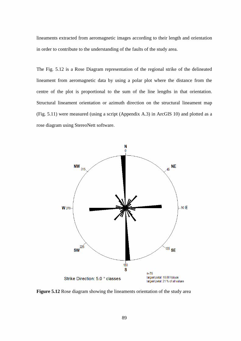
89

lineaments extracted from aeromagnetic images according to their length and orientation

in order to contribute to the understanding of the faults of the study area.

The Fig. 5.12 is a Rose Diagram representation of the regional strike of the delineated

lineament from aeromagnetic data by using a polar plot where the distance from the

centre of the plot is proportional to the sum of the line lengths in that orientation.

Structural lineament orientation or azimuth direction on the structural lineament map

(Fig. 5.11) were measured (using a script (Appendix A.3) in ArcGIS 10) and plotted as a

rose diagram using StereoNett software.

Figure 5.12 Rose diagram showing the lineaments orientation of the study area

90

The rose (azimuth-frequency) diagram (Fig. 5.12) depicted most (major) of the lineament

extracted trends in the north-south (N-S) and east-west (EW) direction with the minor

trending in northeast southwest (NE-SW) and northwest-southeast (NW-SE) direction.

According to Junner (1940); Jones (1990); Blay (2003) the the structures in the area are

complex and most of lineatemt trends in the N-S direction. This accounts for the

observedstructures in the Rose diagram which show that the largest petral is 21 % of the

delinaeted lineaments and represent lineaments trending in the north-south direction. The

Fig. 5.12 also indicates that out of delineated lineaments plotted 11% represented the

second largest petal striking in the east-west (EW) direction, with 6% also striking in the

northeast-southwest (NE-SW) and another 6 % trending in the northwest-southeast (NW-

SE) direction. From the rose diagram it is seen that the area is dominated by a north-south

and east-west trending lineament.

Figure 5.13 is the interpreted lithological map of the area from the aeromagnetic data

showing the shale, sandstone, jasper, basalt and it associate volcanic rocks, Volcanic

domain, part of the Voltaian sediments, and some geological structures. The strike of the

rock formation South-North, SN (Bell & Crook, 2003) of the area is observed.

91

Figure 5.13 Interpreted lithological map from aeromagnetic dataset

The interpreted geological map (Fig. 5.13) from aeromagnetic dataset shows the

lithological units and their contacts and the structures in the Buem formation. The map

(Fig. 5.13) also depicts most of the observations and feature described in the previous

section (section 5.1.1 – 5.1.7).

5.3 Radiometric Data

Radiometric data has many uses including soil mapping and to some extent structural

mapping but its main use is mapping lithological units and alterations by determining the

spatial correlation existing between the radiometric data and the rocks (Gunn et al.,

92

1997b). The spatial correlation of the radiometric data involves measuring of naturally

occurring radioactive elements that exist in minerals forming rock and soil (Telford et al.,

1990). The images generated from the data were analysed and interpreted to provide

geological meaning to the radiometric dataset. Interpretation of these figures and maps

were carried out visually to identify and characterize lithology and delineate possible

surface geological structures. High radiometric elemental patterns and irregular low

magnetic zones are interpreted to have resulted from possible mineral deposits or rock

alterations (Gunn et al., 1997b).

5.3.1 Potassium

The potassium, K, map (Fig. 5.14) shows different degrees of potassium concentrations

that reflects different lithological units and alterations in the area. Potassium radiation

fundamentally comes from potash feldspars, which are mainly common in felsic igneous

rocks (e.g. granite) and are low in mafic rocks (e.g. basalts and andesite) (Gunn et al.,

1997b). Rock alterations can also result in high K concentrations (Wilford et al., 1997).

A number of potassium anomalies are evident in the radiometric image Fig. 5.14. The

colour blue corresponds with low K values whilst the pink corresponds with very high K

values. The colour red represents moderately high to high K values and the shades of

orange to yellow colour represent or are associated with moderately low K values.

Low potassium concentration is observed at the left side of the image (VL), and similar

observation is seen at the upper left corner of the area. This observation coincides with

the Volta Lake (from Fig 1.1) which is observed in the study area. Low concentration was

recorded because water body shields the potassium radiation from the underlying rocks

93

hence, reducing the intensity of the signal at that point. Since radiometric survey uses the

assumption of residual of soil the top 30 cm soil is able to adsorb most of the radiated

radioactive element from the underlying rocks or the lithology. High concentration of K is

also observed at the south-west corner (B in Fig. 5.14) of the area. B is suspected to be

basalt described by Jones (1990); Osae et al., (2006) as being alkaline and having high

concentration of K. High concentration of potassium concentration is found at the central

(BSH in Fig. 5.14) part of the area. This coincides with the shale region mapped in the

analytical signal map (Fig. 5.5) of the magnetic data. This shows that the shale in the area

has high concentration of K and this can be attributed to the description given by Osae et

al., (2006) concerning Buem shale. Osae et al., (2006) described shale in the area as

emitting more gamma rays than other sedimentary rocks in the area. Similar observation

at the center of the area is seen at the southern part (BSH) of the area and this can also be

attributed to the Buem shale.

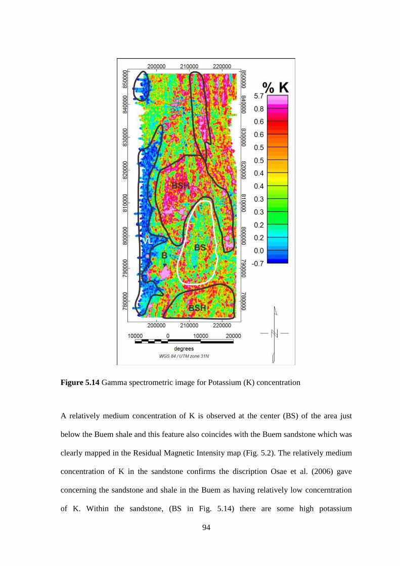
94

Figure 5.14 Gamma spectrometric image for Potassium (K) concentration

A relatively medium concentration of K is observed at the center (BS) of the area just

below the Buem shale and this feature also coincides with the Buem sandstone which was

clearly mapped in the Residual Magnetic Intensity map (Fig. 5.2). The relatively medium

concentration of K in the sandstone confirms the discription Osae et al. (2006) gave

concerning the sandstone and shale in the Buem as having relatively low concerntration

of K. Within the sandstone, (BS in Fig. 5.14) there are some high potassium

95

concerntration which looks almost like a linear feature. This can be attributed to linear

sturcture in the area. It was also observed that the high concentration of potassium

coincides with the elevated region in DEM (Fig. 5.1). The lithological contacts are not

clearly seen in the potassium image.

5.3.2 Thorium

Anomalies in the thorium data in Fig. 5.15 helped map the lithology and lithological

boundaries of the area. The thorium, Th map shows three distinct regions of thorium

concentration in the area. These Th concentration zones are represented by pink colour,

relatively high concentration of the Th concentration represented by green colour and low

Th concentration represented by blue colour (Fig. 5.15). The high concentration in Th

marked by black polygon (Fig. 5.15) correspond to the shale and other weathered

sediment in the area. These weathered sediments are believed to have originated from the

rock (sandstone) in the high elevated lands in the region (Jones, 1990). The assertion is

approved by (Fig. 2.3) and this coincides with the high elevated lands in the area (from

DEM Fig. 5.1). Prominent of this relatively high Th anomaly is observed around the

Alavanyo high lands. Moreover, the low concentration of Th marked by white polygon

observed at the western part of the area coincides with the Volta Lake in the area. This

indicates the fact that the water body shield the emission of radiation from radiogenic

element (thorium) of the underlying lithology.

Weathered sedimentary rocks from the high elevated lands (from DEM Fig. 5.1) for most

part of the area are depicted by high Th radiogenic emissions (red colour). This indicates

the relatively high clay content of the weathered sediment and the adsorption of Th by the

essential clay minerals of the weathered sediments (Blay, 2003). The low K signature

96

recorded may be due to continued weathering and leaching of the sandstone (associated

with the high elevated lands) in most part of the area.

Figure 5.15 Gamma spectrometric image for thorium (eTh) concentration

97

5.3.3 Uranium

The uranium image shows good definition in mapping the Volta Lake (marked by black

polygon in Fig. 5.16) and certain geological formations such as B and BSH. The feature

B, registered high uranium concentration. Interestingly, the circular body (B) which is

observed in the Th and potassium map is also observed in the uranium map. The feature

coincides with the Basalt which Jones (1990) described to be located around that part of

the area. High concentration of uranium is also observed at the central part of the area

marked with a white polygon. This feature coincides with the shale in the area. Thus the

shale is broadly represented by high U concentration (white polygon in Fig. 5.16).

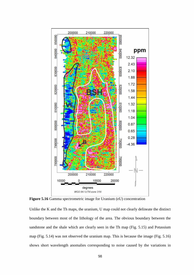
98

Figure 5.16 Gamma spectrometric image for Uranium (eU) concentration

Unlike the K and the Th maps, the uranium, U map could not clearly delineate the distinct

boundary between most of the lithology of the area. The obvious boundary between the

sandstone and the shale which are clearly seen in the Th map (Fig. 5.15) and Potassium

map (Fig. 5.14) was not observed the uranium map. This is because the image (Fig. 5.16)

shows short wavelength anomalies corresponding to noise caused by the variations in

99

atmospheric radon concentrations during the course of the survey resulting in significant

streaking in the image. This is a typical feature found in uranium images (Minty, 1997),

in spite of the processing steps the dataset was subjected to.

5.3.4 Ternary map

The radiometric data are displayed as a ternary map with combined intensities of

potassium (K), thorium (Th), uranium (U) concentration given in red, green, and blue

colour respectively. The ternary radiometric map (Fig. 5.17) shows different colour

combinations which indicate the K, Th and U concentrations. The radiometric responses

in the ternary map, to some extent, correspond with the surface geological map of the

study area (Fig. 2.3). Low concentrations of U, Th, and K radioactive elements are

displayed by black colours with the magenta colour corresponding to high potassium with

low uranium and thorium concentrations. Those with the low content of K but high

contents of U and Th are characterized by green colour and the yellow colours are

characterized by high potassium and thorium with low uranium. Additionally, the blue

colour corresponds to regions of high uranium with low potassium and thorium.

From the ternary map, the Volta Lake can easily be delineated as having low

concentration of the three radiogenic elements (depicted by a black colour in Fig. 5.17).

The contact between the shale and sandstone (C in Fig. 5.17) in the area is also observed.

The high concentration of K, Th and U, marked with the black polygon coincide with the

shale and weathered sediment in the area which Osae et al. (2006) and Jones (1990)

described to be in the area. Osae et al. (2006) and Jones (1990) described the shale in the

area as emitting more gamma rays than other sedimentary rock in the area. The high K

with low U and Th concentration which was depicted by a magenta colour coincides with

100

sandstone in the area and interestingly it also coincides with the high elevated land in the

area. Osae et al. (2006) reported that the sandstones in the area are normaly found at the

highlands or the elevated regions in the area.

Figure 5.17 Ternary map of Study area (RGB=KThU)

The feature (B in Fig. 5.17) with high concentation of the K, U and Th is observed at the

south western part of the area. The feature is seen in all the three radiogenic maps and is

interpreted as the basalt that Osae et al. (2006) and Jones (1990) described in the area.

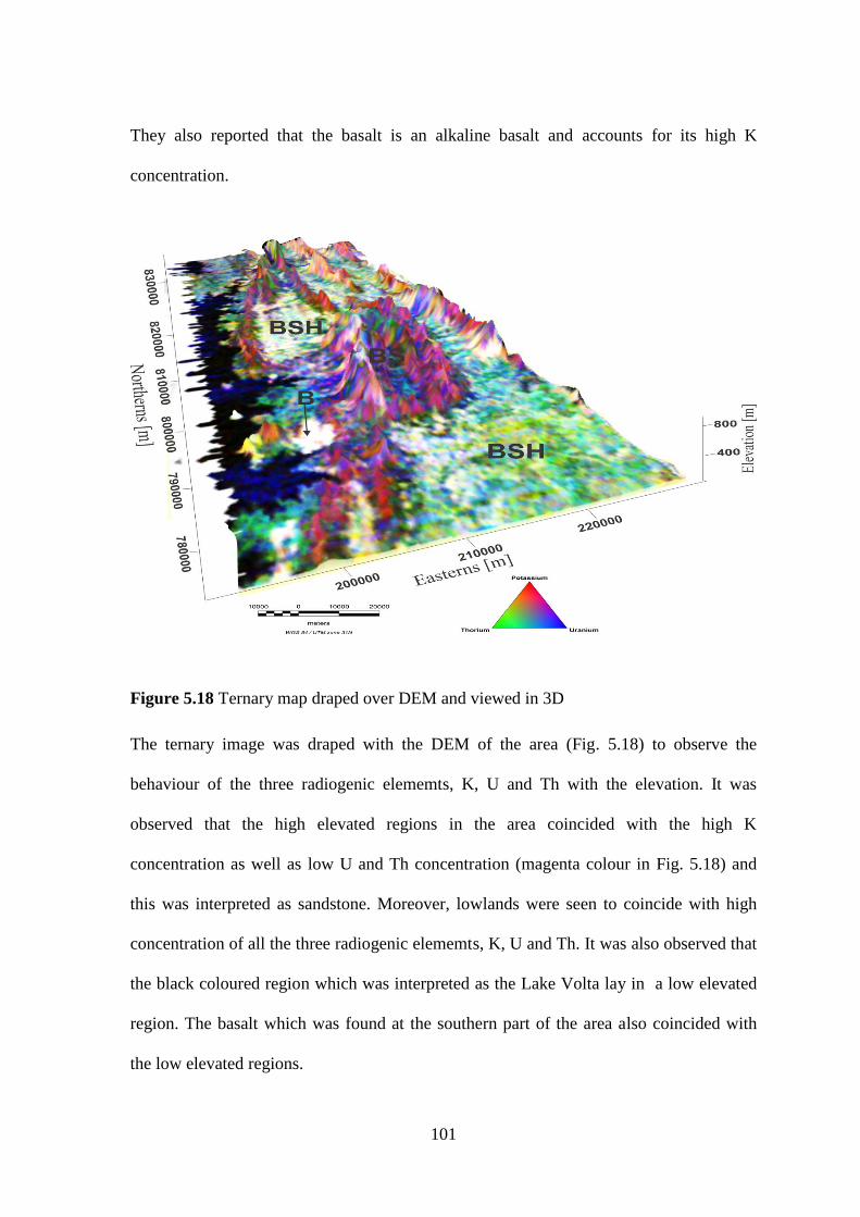
101

They also reported that the basalt is an alkaline basalt and accounts for its high K

concentration.

Figure 5.18 Ternary map draped over DEM and viewed in 3D

The ternary image was draped with the DEM of the area (Fig. 5.18) to observe the

behaviour of the three radiogenic elememts, K, U and Th with the elevation. It was

observed that the high elevated regions in the area coincided with the high K

concentration as well as low U and Th concentration (magenta colour in Fig. 5.18) and

this was interpreted as sandstone. Moreover, lowlands were seen to coincide with high

concentration of all the three radiogenic elememts, K, U and Th. It was also observed that

the black coloured region which was interpreted as the Lake Volta lay in a low elevated

region. The basalt which was found at the southern part of the area also coincided with

the low elevated regions.

102

5.3.5 Summary

Interpreted lithological map from the radiometric dataset combines information from the

uranium image (Fig. 5.16), potassium image (Fig. 5.14), thorium image (Fig. 5.15) and

the ternary image (Fig. 5.17) alongside published articles and geological map of the area.

The area was divided into radiometric domains (regions) based upon the concentration,

shape and abrupt change of radiometric concentration in the radiometric image.

Boundaries of the individual lithological domains are seen as abrupt changes in the

signature of radiometric concentration.

103

Figure 5.19 Interpreted lithological map from the radiometric dataset

The interpreted lithological map Fig. 5.19 of the area from the radiometric dataset shows

the shale (BSH), sandstone (BS), basalt intrusion (B) and part of the Voltaian sediment

(VS). The map Fig. 5.19 also depicts most of the observations and feature described in the

previous sections (section 5.2.1 – 5.2.4).

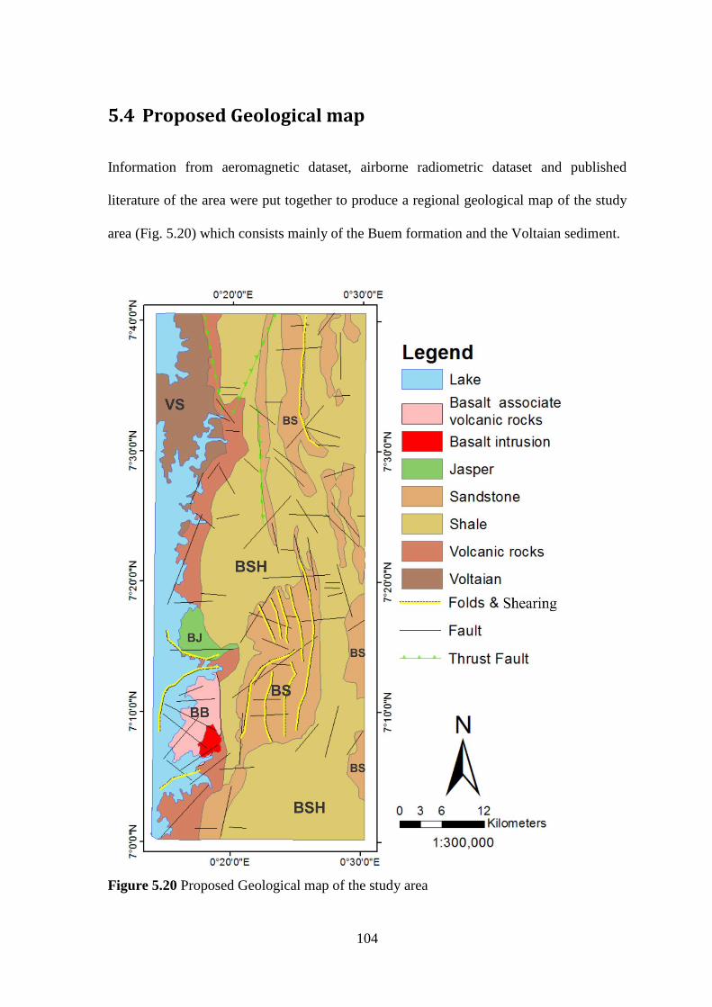
104

5.4 Proposed Geological map

Information from aeromagnetic dataset, airborne radiometric dataset and published

literature of the area were put together to produce a regional geological map of the study

area (Fig. 5.20) which consists mainly of the Buem formation and the Voltaian sediment.

Figure 5.20 Proposed Geological map of the study area

105

The integrated geological map (figure 5.20) shows the various lithological units and the

geological structures in the area. It can be observed from this map (fig. 5.20) that the

Buem sandstones (BS) are associated with different regimes of tectonic activities

producing faults and folds. This can be attributed to the thermo-tectonic event that

occurred within the Buem formation about 600 m.a. (Kennedy, 1964; Jones, 1990; Osae

et al., 2006).

5.5 Quantitative interpretation

Attempt was made to estimate the depth to basement of the magnetic body. The Geosoft

oasis montaj Depth to Basement extension which determines the position (distance along

the profile and depth), dip (orientation) and intensity (susceptibility) of magnetic source

bodies for a magnetic profile was used. The Werner deconvolution function which uses

the horizontal and vertical derivatives in the calculation in the depth to basement of the

magnetic anomaly was employed. It assumes the source bodies are either dikes or

contacts with infinite depth extent and uses a least-squares approach to solve for the

source body (Ku & Sharp, 1983).

Three profiles were chosen across the residual aeromagnetic intensity map of the area to

estimate the depth to magnetic bodies and possibly the intensity (susceptibility), namely

A-A1, B-B1 and C-C1 (Fig. 5.21). They were taken perpendicular to the most prominent

strike direction (N-S) of the anomaly to obtain the best estimate of body parameters from

the selected profiles. The afore-mentioned profiles lines were plotted and displayed on

analytical signal image (Fig. 5.21). Two depth source models (Dike and contacts model)

106

were assumed and their depths to basement were estimated using the Werner

deconvolution function.

Figure 5.21 Profiles lines A-A1, B-B1 and C-C1 displayed on analytical signal image

The profile A-A1 (Fig. 5.22) is a 30-km section of a flight line which cuts the shale,

sandstone and the basalt in the area and runs east to west. For profile A-A1, 106 solutions

were generated with the dike model and the model for the contact generated 72 and 34

solutions respectively. The depth to basement of A-A1 ranged from 103.11 m to 857.99 m

and the magnetic anomaly values varied from -1140.27 nT to -1327.13 nT. The depth to

107

basement of the contact model was shallow (103.11 to 717 m) as compared to the dike

model (114.41 to 857.99 m).

Figure 5.22 Werner deconvolution solutions from a magnetic profile A-A1 over the study

area: (a) residual magnetic intensity profile [nT], (b) depth [m], (c) susceptibility contrast

[SI]. (d) A simplified geological section of the interpreted geological map

The profile B-B1 (Fig. 5.23) is also a 30-km section of a flight line which cuts the

sandstone, shale and the jasper in the area and runs east to west. Additional, for profile B-

B1, 139 solutions were generated with the dike model and the contacts model generated

98 and 41 solutions respectively. The depth to basement of B-B1 ranged from 100.36 m to

1866.34 m with the magnetic anomaly values varying from -1214.33 nT to -1397.33 nT.

The depth to basement of the contact model was shallow (100.36 to 983.71 m) as

compared to the dike model (101.5 to 1866.334 m).

108

Figure 5.23 Werner deconvolution solutions from a magnetic profile B-B1 over the study

area: (a) residual magnetic intensity profile [nT], (b) depth [m], (c) susceptibility contrast

[SI]. (d) A simplified geological section of the interpreted geological map

The profile C-C1 (Fig. 5.24) is also a 30-km section of a flight line which cuts the

Voltaian, shale and the sandstone in the area and runs west to east. Profile C-C1 generated

73 solutions with the dike model and the contacts model generated 45 and 28 solutions

respectively. The depth to basement of C-C1 ranged from 113.82 m to 1605.24 m with the

magnetic anomaly values varying from -1270.13 nT to -1302.81 nT. The depth to

basement of the contact model was shallow (113.82 to 846.28 m) as compared to the dike

model (131.82 to 1605.24 m).

109

Figure 5.24 Werner deconvolution solutions from a magnetic profile C-C1 over the study

area: (a) residual magnetic intensity profile [nT], (b) depth [m], (c) susceptibility contrast

[SI]. (d) A simplified geological section of the interpreted geological map.

From the three profiles it is observed that the depth to basement of the contact model was

shallow (ranging from 100.36 m to 983.709 m) as compared to the dike model (ranging

from 101.15 m to 1866.34 m) and this confirms a similar observation Mushayandebvu et

al., (2001) made in their work work on Great Dyke of Zimbabwe and Teisseyre–

Tornquist Zone, Poland.

110

CHAPTER SIX

6 CONCLUSION AND RECOMMENDATIONS

6.1 Conclusion

In order to map the lithology and geological structures of the study area, airborne

radiometric and magnetic datasets collected over the area were processed and enhanced.

The magnetic image enhancing filters applied to the residual magnetic intensity (RMI)

using Geosoft (Oasis Montaj) are reduction to the pole (RTP), analytic signal, first

vertical derivative (1VD), Tilt derivative (TDR) and upward continuation (UC). These

filters helped define the lithological boundaries, intersection of geological structures,

faults, folds and contacts. The tilt derivative (TDR) proved very useful in the delineation

of the contacts and the most of geological structures in the area. The radiometric data

provided geochemical information of uranium (U), thorium and potassium (K) and

proved valuable in delineating bedrock lithology of the area such as the Buem shale,

sandstone, and part of the Voltaian sediments. The radiometric dataset was also valuable

in the delineation of the Volta Lake and the lithological contacts of the various rock

formations. The interpretation of the high-resolution airborne magnetic dataset has

provided a synopsis of the regional geology (lithology) as well as further insight into

structural controls of the area. It also shows a detailed assessment of various lithology and

north-south striking of the geology in the area.

Most of the delineated structures found within the sandstone, (BS) (at the central and

eastern part of the area), volcanic rocks and the basalt (western part of the area) strike

mostly in the N-S and E-W direction. The jasper deposits which for the past years proved

111

difficult in mapping using this data has been successfully mapped from the enhanced

magnetic dataset. This deposit occurs at the western part of the study area, around

Kwamekrom and Odumase Township (Fig. 1.1), labelled BJ on the interpreted geological

map (Fig. 5.20). The relatively high magnetic signature that the jasper produced

compared with the shale and the sandstone as a result of it being interbedded with iron

oxide (Jones, 1990) helped in delineating the deposit. The Buem sandstone delineated (at

the central and eastern part of the area) produced relatively high magnetic signature. This

may be due to the presence of high composition of magnetic minerals mainly magnetite in

this unit.

The depth to basement of the formations within the study area was determined using the

contact model and the dike models. The contact model produced shallow depth ranging of

100.36 m to 983.709 m while the dike model on the other hand produced depth range of

101.15 m to 1866.34 m for the basement rock. This is because dike model anomaly

occurs at a greater depth than the contact model (Mushayandebvu et al., 2001). The dike

model seems to best fit the study area. The aeromagnetic dataset proved valuable in the

delineation of most of the lithologies and structures in the area and estimating the depth to

basement of the magnetic body with the radiometric dataset proving to be a valuable tool

for mapping lithology and water bodies.

112

6.2 Recommendations

Based on this study, the following recommendations are made:

Ground thrusting is highly recommended to actually confirm the delineated structure and

lithology delineated. Ground geophysical and geological drilling surveys are

recommended where possible to validate airborne geophysical measure since they have

better depth and lateral resolutions.

High structural connectivity regions such as the sandstone region (BS) which has high

potassium, K concentration and relatively low magnetic anomaly (indicating alteration

zone) should be considered for further exploration.

Attempt should be made to model the various lithological units in the study area using the

magnetic data. This data can also be supplemented with 3D electrical resistivity over the

area to map the jasper deposit since it is known to be highly resistive (Jones, 1990).

113

References

Afenya, P. (1982). Ghana‘s mineral resources for small-scale mining industries. (J.

Neilson, Ed.) Strategies for small-scale mining and mineral industries, 8, 24-28.

Affaton, P., Sougy, J., & Trompette, R. (1980). The tectono-stratigraphic relationships

between the Upper Precambrian and Lower Paleozoic Volta basin and the Pan-

African Dahomeyide orogenic belt (West Africa). American Journal of Science,

280, 224-248.

Airo, M. (2005). Regional interpretation of aerogeophysical data: extracting

compositional and structural features. Geological Survey of Finland, Special

Paper, 39, 176–197.

Airo, M. L. (2002). Aeromagnetic and aeroradiometric response to hydrothermal

alteration. Surveys in Geophysics, 23, 273–302.

Airo, M., & Loukola-Ruskeeniemi, K. (2003). Characterization of sulfide deposits by

airborne magnetic and gamma-ray responses in eastern Finland. Ore Geology

Reviews, 24, 67–84.

Amoako, P. Y., Amedofu, S. K., & Akamaluk, T. (l998). Processing and Interpretation of

Data from Airborne Geophysical Survey, Ghana Final Report. Geological Survey

Department of Ghana. Accra: Geological Survey Department of Ghana.

Asadi, H., & Hale, M. (1999). Integrated analysis of aeromagnetic, landsat TM and

mineral occurrence data for epithermal gold exploration in northwest iran.

13th International Conference on Applied Geologic Remote Sensing,

Vancouver. British Columbia.

Atchuta Rao,, D., & Ram Badu, H. (1981). Nomograms for rapid evaluation of magnetic

anomalies over long tabular bodies. Pure and Applied Geophysics, 119, 1037-

1050.

Bell, S. V. (1962). Ghana Geological Survey Annual Report. Accra: Ghana Geological

Survey.

114

Bell, S., & Crook, J. (2003). The Geology of 1/4 Feild Sheets 182, Hohoe S. E with a

contribution on the structural Relationship to Kpandu-Ho Area. Accra: Ghana

Geological Survey Department.

Beltrão, J., Silver, J., & Costa, J. (1991). Robust polynomial fitting method for regional

gravity estimation. Geophysics, 56, 80–9.

Billings, S. (1998). Geophysical aspects of soil mapping using airborne gamma-ray

spectrometry.

Blay, P. (2003). The Geology of 1/4 Feild Sheets Nos. 184, 185 and 187, Hohoe N. E.,

Baglo S.W. and N.W. Accra: Ghana Geological Survey Department .

Briggs, I. (1974). Machine contouring using minimum curvature. Geophysics, 39(1), 39-

48.

Chandler , V. (1990). Geological interpretation of gravity and magnetic data over the

central part of the Duluth Complex northeastern Minnesota. Economic Geology,

85, 861-829.

Clark, D. (1997). Magnetic properties of rocks and minerals. AGSO Journal of Australian

Geology and Geophysics, 17(2), 83-103.

Cooper, G., & Cowan, D. (2006). Enhancing potential field data using filters based on the

local phase. Computers & Geosciences, 32, 1585–1591.

Dapaah-Siakwan, S., & Gyau-Boakye, P. (2000). Hydrogeologic framework and borehole

yields in Ghana. Hydrogeology Journal, 8, 405–416.

Delor, C., Fullgraff, T., Urien, P., Le Berre, P., Thomas, E., Roig, J., et al. (2009).

Geological Map Explanation – Map Sheets 0700A/2, 0700B/1, 0800D/1, 0800D/3,

0800C/2 & 0800C/4. Accra: Geological Survey Department of Ghana (GSD).

Dickson, B., & Scott, K. (1997). Interpretation of aerial gamma-ray surveys adding the

geochemical factors. AGSO Journal of Australian Geology & Grophysics., 17(2),

187-200.

115

Dickson, K., & Benneh, G. (1985). A New Geography of Ghana. England: Longman

House, Burnt Mill, Harlou, Essex.

Direen, N. G., Lyons, P., Korsch, & Glen, R. (2001). Integrated geophysical appraisal of

crustal architecture in the eastern Lachlan Orogen. Exploration Geophysics, 109,

136-142.

Dobrin, M., & Savit, C. (1988). Introduction To Geophysical Prospecting (Fourth Edition

ed.). Singapore: McGraw-Hill.

Duffett, M. (1998). Gravity, magnetic and radiometric evidence for the geological setting

of the Lady Loretta Pb-Zn-Ag deposit - a qualitative appraisal. Economic

Geology, 93, 1295-1306.

Eisenlohr, B., & Hirdes, W. (1992). The structural development of the early Proterozoic

Birimian and Tarkwaian rocks of southwest Ghana. West Africa. Journal of

African Earth Sciences, 14(3), 313-325.

El-awady, M., El-etr, H., & Bakrah, A. (1984). Aeromagnetic geophysical investigation

in El-Faiyum district, western desert, Egypt. Qatar Univ. Sci. Bull, 5, 335-357.

Fertl, W. (1983). Gamma-ray spectral logging: a new evaluation frontier. World Oil, 79-

91.

Foss, C. (2011). Magnetic data Enhancement and Depth Estimation. (H. Gupta, Ed.)

Encyclopedia of Earth Sciences Series, 736-746.

Galbraith, J. H., & Saunders, D. F. (1983). Rock classification by characteristics of aerial

gamma-ray measurements. Journal of Geochemical Exploration, 18(1), 49-73.

Geotech Airborne Limited. (2009). Integrated Interpretation Report on a Versatile Time

Domain Electromagnetic (VTEM) Survey on the Hohoe Project Area. Geological

Survey Department, Accra, Ghana.

Ghana Statistical Service. (2012). 2010 Population and Housing Census (PHC). Ghana

Statistical Service, Accra.

116

Grant, F., & Martin, L. (1966). Interpretation theory in applied Geophysics. New York:

McGraw-Hill Book Co.

Gregory, A., & Horwood, J. (1961). A laboratory study of gamma-ray spectra at the

surface of rocks. Ottowa: Department of Energy, Mines and nnnResources.

Griffis, R. J., Barning, K., Agezo, F. L., & Akosah, F. K. (2002). Gold Deposits of

Ghana. Accra, Ghana: Minerals Commission.

GSD. (1988). Geological Map of Ghana (1:1 000 000) with mineral deposits. Geological

Survey Department of Ghana, Accra.

Guillemot, D. (1987). Airborne magnetometer and spectrometer survey over Gabon. First

Break, 5(7).

Gunn, P. (1997). Regional magnetic and gravity responses of extensional sedimentary

Basins. AGSO Journal of Australian Geology & Geophysics, 17(2), 115-131.

Gunn, P., Maidment, D., & Milligan, P. (1997a). Interpreting aeromagnetic data in areas

of limited outcrop. AGSO Journal of Australian Geology & Geophysics, 17(2),

175–185.

Gunn, P., Minty, B., & Milligan, P. (1997b). The Airborne Gamma-Ray Spectrometric

Response Over Arid Australian Terranes. In A. Gubins (Ed.), Proceedings of

Exploration 97: Fourth Decennial International Conference on Mineral

Exploration, (pp. 733-740). Australia.

Hardy, S. (2004). The Application and Analysis of Airborne Gamma Spectrometry

(Radiometrics) for Mapping Soils in Central Queensland. ISCO 2004 - 13th

International Soil Conservation Organisation Conference. Brisbane, Australia.

Hasting, D. (1982). On the tectonics and metallogenesis of West Africa: A model

incorporating new geophysical data. Geoexploration, 20, 295-327.

Hirdes, W., Davis, D., & Eisenlohr, B. (1992). Reassessment of Proterozoic granitoid

ages in Ghana on the basis of U/Pb zircon and monazite dating. Precambrian

Research, 56, 89-96.

117

Hirst, T. (1946). Reports on the Bibiani goldfield, Part I: The geology of the field. Accra:

Gold Coast Geological Survey Department.

Hoffman, P. (1999). The break-up of Rodinia, birth of Gondwana, true polar wander and

the snowball Earth. Journal of African Earth Sciences, 28, 17-33.

Holm, R. (1974). Petrology of alkalic gneiss in the Dahomeyan of Ghana. Geological

Society of America Bulletin, 85, 1441-1448.

Jones, W. (1990). The Buem volcanic and associated sedimentary rocks, Ghana: a field

and geochemical investigation. Journal of African Earth Sciences, 11(3–4), 373-

383.

Junner. (1940). The Geology of the Gold Coast and western Togoland. Gold Coast

Geological Survey Bulletin, 11, 1-40.

Junner, N. (1935). Gold in gold coast. Accra, Ghana: Geological Survey Department.

Kennedy, W. (1964). The structural differentiation of Africa in the Pan-African (±500

m.y.) tectonic episode. UK: Leeds University Institute for African Geology.

Kesse, G. (1985). The mineral and rock resources of Ghana. United States: A.A.

Balkema Publishers,Accord, MA.

Koulomzine, T., Lamontagne, Y., & Nadeau, A. (1970). New methods for the direct

interpretation of magnetic anomalies caused by inclined dykes of infinite length.

Geophysics, 35, 812-830.

Ku, C., & Sharp, J. (1983). Werner deconvolution for automated magnetic interpretation

and its refinement using Marquart's inverse modeling. Geophysics, 48(6), 754-

774.

Leube, A., Hirdes, W., Mauer, R., & Kesse, G. (1990). The early proterozoic Birimian

supergroup of Ghana and some aspects of its associated gold mineralisation.

Precambrian Research, 46, 139-165.

Li, X. (2008). Magnetic reduction-to-the-pole at low latitudes. Fugro Gravity and

Magnetic Services. Houston, USA.: Fugro .

118

LUO, Y., XUE, D.-J., & WANG, M. (2010). Reduction to the Pole at the Geomagnetic

Equator. Chinese Journal of Geophysics, 53(6), 1082-1089.

Mani, R. (1978). The geology of the Dahomeyan of Ghana; Geology of Ghana Project.

Accra: Ghana Geological Survey Department.

Miller, H., & Singh, V. (1994). Potential field tilt—a new concept for location of

potential field sources. Journal of Applied Geophysics, 32, 213–217.

Milligan, P., & Gunn, P. (1997). Enhancement and presentation of airborne geophysical

data. AGSO Journal of Australian Geology & Geophysics, 17(2), 63-75.

Milsom, J. (2003). Field Geophysics. (Third, Ed.) London: Wiley.

Minty, B. (1997). Fundamentals of airborne gamma-ray spectrometry. AGSO Journal of

Australian Geology & Geophysics., 17(2), 39-50.

Misener, D. (1987). Interpretation of airborne geophysical survey results. Toronto,

Canada: Paterson, Grant & Watson Ltd.

Murphy, B. (2007). Airborne geophysics and the indian scenario. Journal of Indian

Geophysics, 11(1), 1–28.

Murray, R. (1960). The geology of the "Zuarungu" 1/2° Field Sheet. Accra: Ghana

Geological Survey Department Bulletin No.25.

Mushayandebvu, M., van Drielz, P., Reid, A., & Fairhead, J. (2001). Magnetic source

parameters of two-dimensional structures using extended Euler deconvolution.

Geophysics, 66(3), 814–823.

Oruc, B., & Selim, H. (2011). Interpretation of magnetic data in the Sinop area of Mid

Black Sea, Turkey, using tilt derivative, Euler deconvolution, and discrete wavelet

transform. Journal of Applied Geophysics, 74, 194–204.

Osae, S., Asiedu, D., Banoeng-Yakubo, B., Koeberl, C., & Dampare, S. (2006).

Provenance and tectonic setting of Late Proterozoic Buem sandstones of

southeastern Ghana: Evidence from geochemistry and detrital modes. Journal of

African Earth Sciences, 44, 85–96.

119

Ostrovskiy, E. (1975). Antagonism of radioactive elements in wallrock alteration fields

and its use in aerogamma spectrometric prospecting. International Geology

Review, 17(4), 461-468.

Pesonen, L. J., Koeberl, C., & Hautaniemi, H. (2003). Airborne Geophysical Survey of

the Lake Bosumtwi Meteorite Impact Structure. Jahrbuch Der Geologischen

Bundesanstalt, 143(4), 581–604.

PGEO, E. K. (2012). Technical Report on Sheini Hills Iron Project. Canada: Cardero

Resource Corporation.

Philips, J. (1997). Potential-Field Geophysical Software for the PC,. U.S.G.S. Open-File

Report 97-725.

Reeves, C., Reford, S., & Millingan, P. (1997). Airborne geophysics:old methods, new

images. In A. Gubins (Ed.), Proceedings of the Fourth Decennial International

Conference on Mineral Exploration, (pp. 13-30). Australia.

Roest, W., Verhoef, J., & Pilkington, M. (1992). Magnetic interpretaion using 3-D

analytical signal. Geophysics, 57, 116-125.

Roy, A. (1966). The method of continuation in mining geophysics. Geoexploration, 4, 65-

83.

Salem, A., Williams, S., Fairhead, J., Ravat, D., & Smith, R. (2007). Tilt-depth method: a

simple depth estimation method using first-order magnetic derivatives. The

Leading Edge , 26, 1502-1505.

Shi, Z., & Butt, G. (2004). New enhancement filters for geological mapping. 17th

Geophysical Conference and Exhibition. USA: ASEG.

Silva, A., Pires, A., Mccafferty, A., De Moraes , R., & Xia, H. (2003). Application of

Airborne Geophysical Data to Mineral Exploration in the Uneven Exposed

Terrains of the Rio Das Velhas Greenstone Belt. Revista Brasileira de

Geociências, 33, 17-28.

Smith, R., & O‘Connell, M. (2007). An Improved Method for Trending of Features on

Aeromagnetic Maps. In B. Milkereit, (Ed.), Proceedings of Exploration 07: Fifth

120

Decennial International Conference on Mineral Exploration, (pp. 853-861).

Toronto, Canada.

121

Taylor, P., Moorbath, S., Leube, A., & Hirdes, W. (1988). Geochronology and crustal

evolution of Early Proterozoic granite-greenstone terrains in Ghana. West Africa:

in International Conference and Workshop on the Geology of Ghana with Special

Emphasis on Gold, (pp. 43-45). Accra.

Telford, W., Gelbert, I., & Sheritt, R. (1990). Applied Geophysics (Second ed.). London:

Cambridge University Press.

Verduzco, B., Fairhead, J., Green, C., & Mackenzie, C. (2004). New insights into

magnetic derivatives for structural mapping. The Leading Edge, 23, 116-119.

Vernon, R., & Flood, R. (1988). Contrasting deformation of S- and I-type granitoids in

the Lachlan Fold Belt, eastern Australia. Tectonophysics, 147, 127-143.

Villeneuve, M., & Cornée, J. (1994). Structure, evolution and palaeogeography of the

West African Craton and bordering belts during the Neoproterozoic. Precambrian

Research, 69, 307-326.

Wemegah, D., Menyeh, B., & Danuor, S. (2009). Magnetic Susceptibility

Characterization of mineralized and non mineralized rocks of the Subenso

Concession of Newmont Ghana Gold Limited. Ghana Science Association

Biennial Conference. Accra.

Wilford, J., Bierwirth, P., & Craig, M. (1997). Application of airborne gamma-ray

spectrometry in soil or regolith mapping and applied geomorphology. Journal of

Australian Geology & Geophysics, 17(2), 201-216.

Wright. (1985). Geology and Mineral Resources of West Africa. Springer.

Wright, J., Hastings, D., Jones, W., & Williams, H. (1985). Geology and Mineral

Resources of West Africa. London: George Allen and Unwin publishers Ltd.

122

Appendix

Appendix A 1 Generation of Werner deconvolution

solutions

Figure A 1 Parameters dialog box for generating Werner solutions

123

Appendix A.2 Werner deconvolution solutions

Figure A 2 Geosoft Oasis montaj database (GDB) displaying the Werner generated

solutions

Appendix A.3 Script for extracting azimuth of lineaments

import math

def GetAzimuthPolyline(shape):

radian = math.atan((shape.lastpoint.x - shape.firstpoint.x)/(shape.lastpoint.y - shape.firstpoint.y))

degrees = radian * 180 / math.pi

return degrees

__esri_field_calculator_splitter__

GetAzimuthPolyline( !Shape!)

Equation A 1 expression for extracting azimuth direction delineated lineament in ArcGIS

10.