Graduate School ETD Form 9 PURDUE UNIVERSITY GRADUATE ... · Purdue University by Samuel Assegie In...

Graduate School ETD Form 9 (Revised 12/07)

PURDUE UNIVERSITY GRADUATE SCHOOL

Thesis/Dissertation Acceptance

This is to certify that the thesis/dissertation prepared

By

Entitled

For the degree of

Is approved by the final examining committee:

Chair

To the best of my knowledge and as understood by the student in the Research Integrity and Copyright Disclaimer (Graduate School Form 20), this thesis/dissertation adheres to the provisions of Purdue University’s “Policy on Integrity in Research” and the use of copyrighted material.

Approved by Major Professor(s): ____________________________________

____________________________________

Approved by: Head of the Graduate Program Date

Samuel Assegie

Efficient and Secure Image and Video Processing and Transmission in Wireless SensorNetworks

Master of Science in Electrical and Computer Engineering

Brian King

Paul Salama

Maher Rizkalla

Brian King

Brian King 07/27/2010

Graduate School Form 20 (Revised 1/10)

PURDUE UNIVERSITY GRADUATE SCHOOL

Research Integrity and Copyright Disclaimer

Title of Thesis/Dissertation:

For the degree of ________________________________________________________________

I certify that in the preparation of this thesis, I have observed the provisions of Purdue University Teaching, Research, and Outreach Policy on Research Misconduct (VIII.3.1), October 1, 2008.* Further, I certify that this work is free of plagiarism and all materials appearing in this thesis/dissertation have been properly quoted and attributed.

I certify that all copyrighted material incorporated into this thesis/dissertation is in compliance with the United States’ copyright law and that I have received written permission from the copyright owners for my use of their work, which is beyond the scope of the law. I agree to indemnify and save harmless Purdue University from any and all claims that may be asserted or that may arise from any copyright violation.

______________________________________ Printed Name and Signature of Candidate

______________________________________ Date (month/day/year)

*Located at http://www.purdue.edu/policies/pages/teach_res_outreach/viii_3_1.html

Efficient and Secure Image and Video Processing and Transmission in Wireless SensorNetworks


Samuel Assegie

07/09/2010

EFFICIENT AND SECURE IMAGE AND VIDEO PROCESSING AND

TRANSMISSION IN WIRELESS SENSOR NETWORKS

A Thesis

Submitted to the Faculty

of

Purdue University

by

Samuel Assegie

In Partial Fulfillment of the

Requirements for the Degree

of


August 2010

Purdue University

Indianapolis, Indiana

ii

To my family.

iii

ACKNOWLEDGMENTS

Foremost, I would like to express my sincere gratitude to my advisor Prof. Brian

King for his continuous support, patience, motivation and immense knowledge during

my graduate studies. His guidance helped me in all the time of research and writing

of this thesis. I could not have imagined having a better advisor and mentor.

I would like to express my sincere gratitude to Prof. Paul Salama, for his support

in my studies, providing me with research ideas and working with me closely in solving

the problems.

I would like to thank Prof. Dongsoo (Stephen) Kim for his support in my research

and being part of my thesis committee.

I would also like to thank Prof. Lauren Christopher and Prof. Maher Rizkalla for

being part of my thesis defense committee and their positive feedback which helped

me to make my thesis better. I also like to thank Ms. Valerie Lim Diemer for her

help during my studies. I am grateful to all the professors in Electrical and Computer

Engineering Department for their excellent teaching.

Most importantly, none of this would have been possible without the love and

support of my family.

Finally, I appreciate the financial support from Electrical and Computer Engi-

neering Department that funded my research and studies.

iv

TABLE OF CONTENTS

Page

LIST OF TABLES . . . . . . . . . . . . . . . . . . . . . . . . . . . . . . . . vii

LIST OF FIGURES . . . . . . . . . . . . . . . . . . . . . . . . . . . . . . . viii

ABSTRACT . . . . . . . . . . . . . . . . . . . . . . . . . . . . . . . . . . . x

1 INTRODUCTION . . . . . . . . . . . . . . . . . . . . . . . . . . . . . . 1

2 BACKGROUND MATERIAL . . . . . . . . . . . . . . . . . . . . . . . . 4

2.1 Image Compression - Using Wavelets . . . . . . . . . . . . . . . . . 4

2.1.1 Image/Video Compression . . . . . . . . . . . . . . . . . . . 4

2.1.2 Wavelet Coding . . . . . . . . . . . . . . . . . . . . . . . . . 5

2.2 Background Subtraction Method for Detecting Foreground Objects 7

2.2.1 Background Model - Estimating Good Background . . . . . 7

2.2.2 The Most Common Approaches of Background Generation . 8

2.3 Security . . . . . . . . . . . . . . . . . . . . . . . . . . . . . . . . . 10

2.3.1 Cryptography . . . . . . . . . . . . . . . . . . . . . . . . . . 10

2.4 Multimedia Security . . . . . . . . . . . . . . . . . . . . . . . . . . 12

2.4.1 Image/Video Encryption Scheme . . . . . . . . . . . . . . . 12

2.5 Selective Encryption . . . . . . . . . . . . . . . . . . . . . . . . . . 13

3 SELECTIVE ENCRYPTION . . . . . . . . . . . . . . . . . . . . . . . . 14

3.1 Introduction . . . . . . . . . . . . . . . . . . . . . . . . . . . . . . . 14

3.2 Wavelet Based Compression Techniques . . . . . . . . . . . . . . . . 15

3.3 Prior Work on Selective Encryption . . . . . . . . . . . . . . . . . . 17

4 ATTACKING WAVELET TREE SHUFFLING ENCRYPTION SCHEME 20

4.1 A Generic Framework of a Wavelet Tree Shuffling Encryption Scheme 20

4.2 Attacking a Wavelet Tree Shuffling Encryption Scheme . . . . . . . 22

5 DESIGN MODEL . . . . . . . . . . . . . . . . . . . . . . . . . . . . . . . 27

v

Page

5.1 Introduction - Design Summary . . . . . . . . . . . . . . . . . . . . 27

5.2 Design Goal . . . . . . . . . . . . . . . . . . . . . . . . . . . . . . . 27

5.3 Where Does the Power Go? . . . . . . . . . . . . . . . . . . . . . . 29

5.4 Energy/Power Analysis of Sensor Nodes . . . . . . . . . . . . . . . 31

5.4.1 In-Sensor (Node Level) Energy Optimization . . . . . . . . . 31

5.4.2 Network-Wide Energy Optimization . . . . . . . . . . . . . . 32

5.5 System Model . . . . . . . . . . . . . . . . . . . . . . . . . . . . . . 32

5.6 Network Assumption . . . . . . . . . . . . . . . . . . . . . . . . . . 32

5.7 Node Power Consumption Model . . . . . . . . . . . . . . . . . . . 33

5.8 Our First Design . . . . . . . . . . . . . . . . . . . . . . . . . . . . 34

6 ENCODER . . . . . . . . . . . . . . . . . . . . . . . . . . . . . . . . . . 36

6.1 Introduction . . . . . . . . . . . . . . . . . . . . . . . . . . . . . . . 36

6.1.1 Principles of Image Compression . . . . . . . . . . . . . . . 36

6.1.2 Classification of Compression Technique . . . . . . . . . . . 36

6.1.3 Model/Framework of General Image Compression Method . 37

6.1.4 Wavelets for Image Compression . . . . . . . . . . . . . . . . 39

6.2 Haar Wavelet Technique . . . . . . . . . . . . . . . . . . . . . . . . 41

6.2.1 Haar Example . . . . . . . . . . . . . . . . . . . . . . . . . . 41

6.2.2 Filter Banks . . . . . . . . . . . . . . . . . . . . . . . . . . . 42

6.2.3 Image Thresholding . . . . . . . . . . . . . . . . . . . . . . . 42

6.2.4 Procedures and Experimental Results . . . . . . . . . . . . . 44

6.2.5 Energy Efficient Local Processing Using DWT . . . . . . . . 45

6.3 Background Subtraction Method for Image Compression . . . . . . 51

6.3.1 Background Model - Estimating Good Background . . . . . 52

6.3.2 The Most Common Approaches of Background Modeling . . 52

6.3.3 Foreground Processing . . . . . . . . . . . . . . . . . . . . . 52

6.3.4 Improving the Run Length Encoder . . . . . . . . . . . . . . 53

vi

Page

6.4 Exploiting Data Correlation Between Neighborhood Sensors for EnergyEfficient Data Transmission in WMSN . . . . . . . . . . . . . . . . 55

6.4.1 Block Matching Algorithm . . . . . . . . . . . . . . . . . . . 57

6.4.2 Transmission of Data After Receiving Codebook: Encoder Side 57

6.4.3 The Overall Encoding Process . . . . . . . . . . . . . . . . . 61

7 IMAGE QUALITY ASSESSMENT BY BASE STATION . . . . . . . . . 65

7.1 Introduction . . . . . . . . . . . . . . . . . . . . . . . . . . . . . . . 65

7.2 Image Quality Assessment Tools . . . . . . . . . . . . . . . . . . . . 66

7.3 Reduced-Reference (RR) QA Methods, Our Approach (Technique) . 68

7.3.1 Thumbnail . . . . . . . . . . . . . . . . . . . . . . . . . . . . 69

7.3.2 Evaluating Thumbnail Image Quality . . . . . . . . . . . . . 69

7.4 Statistical Test . . . . . . . . . . . . . . . . . . . . . . . . . . . . . 74

7.4.1 Mean Test . . . . . . . . . . . . . . . . . . . . . . . . . . . . 75

7.4.2 Variance Test . . . . . . . . . . . . . . . . . . . . . . . . . . 76

7.5 Applying Three Metrics for Quality Assessment . . . . . . . . . . . 78

8 DECODER . . . . . . . . . . . . . . . . . . . . . . . . . . . . . . . . . . 85

8.1 Decoding Packets and Coordinating Sensor Operation . . . . . . . . 85

8.1.1 Decoding Packets Received from the Sensor: . . . . . . . . . 85

8.1.2 Block Matching Algorithm (BMA) . . . . . . . . . . . . . . 87

8.1.3 Checking Quality of the Reconstructed Image . . . . . . . . 89

9 Conclusion and Future Work . . . . . . . . . . . . . . . . . . . . . . . . . 92

LIST OF REFERENCES . . . . . . . . . . . . . . . . . . . . . . . . . . . . 94

vii

LIST OF TABLES

Table Page

4.1 Relationship between no. of decomp. and no. of trees for an image of size256× 256 . . . . . . . . . . . . . . . . . . . . . . . . . . . . . . . . . . 24

6.1 Computation cost, DWT (Haar filter) . . . . . . . . . . . . . . . . . . . 47

6.2 Communication Cost, DWT (Haar Filter) . . . . . . . . . . . . . . . . 48

6.3 Simulation result, DWT (Haar filter, L = 2) with global and level depen-dent threshold . . . . . . . . . . . . . . . . . . . . . . . . . . . . . . . . 51

6.4 Encoding foreground image based on 10 neighboring images . . . . . . 55

6.5 Simulation Result: Number of matched blocks between two frames, withdifferent threshold . . . . . . . . . . . . . . . . . . . . . . . . . . . . . 64

7.1 PSNR value of original image vs. thumbnail image . . . . . . . . . . . 74

7.2 Codebook results on traffic.avi video . . . . . . . . . . . . . . . . . . . 81

7.3 Estimating retransmission requests by base station . . . . . . . . . . . 82

7.4 Wavelet transform-2 levels of decomposition . . . . . . . . . . . . . . . 83

7.5 Foreground - RLE with threshold (based on 10 images near background)240× 320 image (300 blocks) . . . . . . . . . . . . . . . . . . . . . . . 84

7.6 RLE with threshold assessing by using only the variance test . . . . . . 84

viii

LIST OF FIGURES

Figure Page

2.1 Encryption and decryption of a cipher . . . . . . . . . . . . . . . . . . 11

3.1 The relations between wavelet coefficients in different subbands as quad-trees as illustrated in [69]. LL1 is the low-low coefficients (that is, low passfiltered in the vertical, and low pass filtered in the horizontal). LH1,HL1,HH1are defined similarly. . . . . . . . . . . . . . . . . . . . . . . . . . . . . 16

4.1 Encrypting by shuffling wavelet trees . . . . . . . . . . . . . . . . . . . 21

4.2 Original image . . . . . . . . . . . . . . . . . . . . . . . . . . . . . . . 25

4.3 Shuffled image where L = 3 . . . . . . . . . . . . . . . . . . . . . . . . 25



5.1 Sensor operation flowchart . . . . . . . . . . . . . . . . . . . . . . . . . 30

5.2 Averaging and differencing to find Haar vectors . . . . . . . . . . . . . 31

5.3 WMSN with 7 sensors and a single sink . . . . . . . . . . . . . . . . . 33

5.4 A fist design of our encoder . . . . . . . . . . . . . . . . . . . . . . . . 35

6.1 A model for lossy image encoder . . . . . . . . . . . . . . . . . . . . . 38

6.2 Wavelet decomposition of Lena (512× 512, L = 3) . . . . . . . . . . . 40

6.3 Computation vs. communication cost, DWT(s = 1,2,3) . . . . . . . . . 50

6.4 Run length encoding, with different divisor (threshold) . . . . . . . . . 56

6.5 Overlap between proximate sensor measurement . . . . . . . . . . . . . 58

6.6 Reference image vs. frame with threshold = 0 . . . . . . . . . . . . . . 60

6.7 Frame with threshold = 3 vs. frame with threshold = 9 . . . . . . . . . 61




6.11 Encoding System . . . . . . . . . . . . . . . . . . . . . . . . . . . . . . 63

ix

Figure Page

7.1 Comparison of image similarity metrics among MSE, PSNR and SSIM 67

7.2 256 × 256 8-bit grayscale girls image with mean thumb image based on4× 4 blocking. . . . . . . . . . . . . . . . . . . . . . . . . . . . . . . . 70

7.3 PSNR: Original-reconstructed vs. thumb version of Orig-rec . . . . . . 71

7.4 Image: Bicycle and its thumbnail version . . . . . . . . . . . . . . . . . 72

7.5 Image: Girls and its thumbnail version . . . . . . . . . . . . . . . . . . 73

7.6 Image: Bicycle modified and its thumbnail version . . . . . . . . . . . . 73

8.1 Decoder design . . . . . . . . . . . . . . . . . . . . . . . . . . . . . . . 86

8.2 Block is moved to all vertical, horizontal, left and right displacements inthe search area (R from all sides of the macro block) until a match isfound with in the given threshold (matching is based on mean absolutedifference). . . . . . . . . . . . . . . . . . . . . . . . . . . . . . . . . . 89

x

ABSTRACT

Assegie, Samuel. M.S.E.C.E., Purdue University, August 2010. Efficient and SecureImage and Video Processing and Transmission in Wireless Sensor Networks . MajorProfessor: Brian King.

Sensor nodes forming a network and using wireless communications are highly use-

ful in a variety of applications including battle field (military) surveillance, building

security, medical and health services, environmental monitoring in harsh conditions,

for scientific investigations on other planets, etc. But these wireless sensors are re-

source constricted: limited power supply, bandwidth for communication, processing

speed, and memory space. One possible way of achieve maximum utilization of those

constrained resource is applying signal processing and compressing the sensor read-

ings. Usually, processing data consumes much less power than transmitting data in

wireless medium, so it is effective to apply data compression by trading computation

for communication before transmitting data for reducing total power consumption by

a sensor node. However the existing state of the art compression algorithms are not

suitable for wireless sensor nodes due to their limited resource. Therefore there is a

need to design signal processing (compression) algorithms considering the resource

constraint of wireless sensors. In our work, we designed a lightweight codec system

aiming surveillance as a target application. In designing the codec system, we have

proposed new design ideas and also tweak the existing encoding algorithms to fit the

target application. Also during data transmission among sensors and between sensors

and base station, the data has to be secured. We have addressed some security issues

by assessing the security of wavelet tree shuffling as the only security mechanism.

1

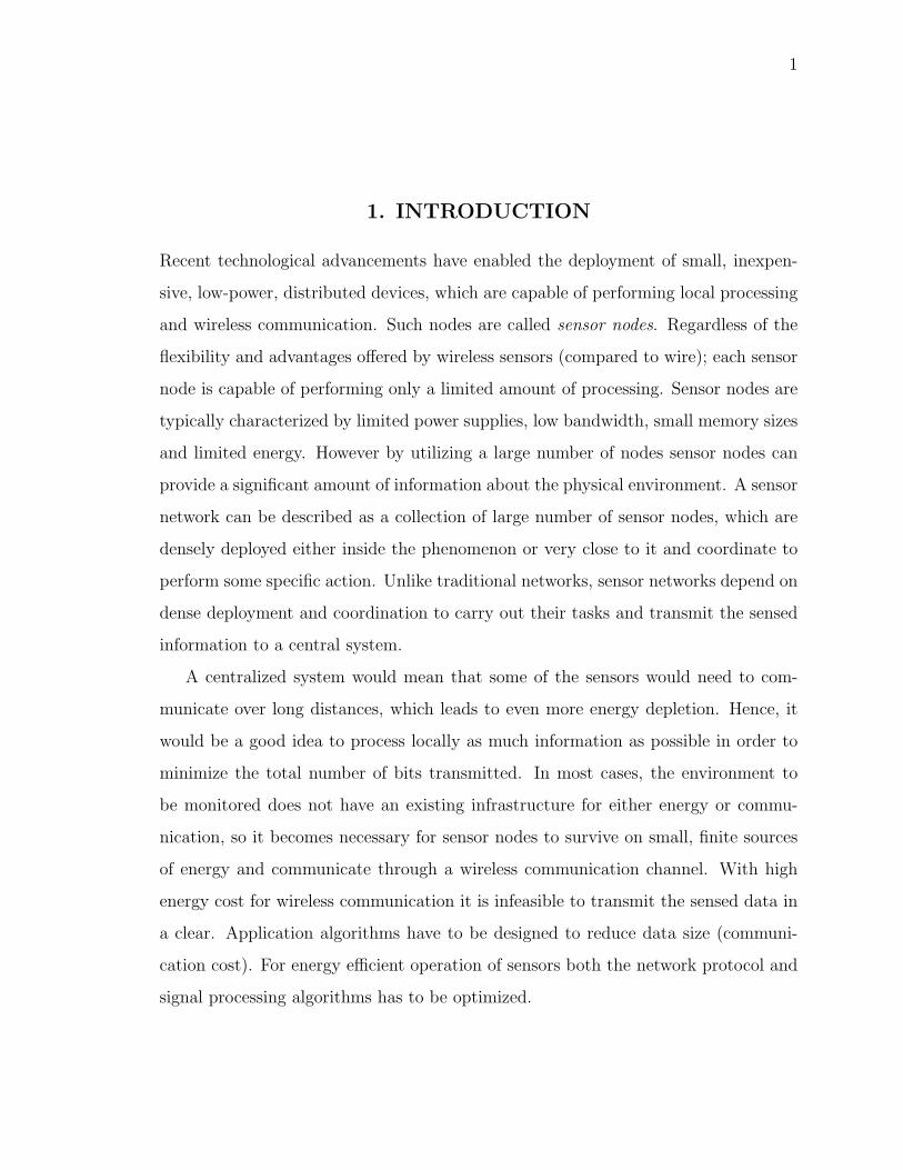
1. INTRODUCTION

Recent technological advancements have enabled the deployment of small, inexpen-

sive, low-power, distributed devices, which are capable of performing local processing

and wireless communication. Such nodes are called sensor nodes. Regardless of the

flexibility and advantages offered by wireless sensors (compared to wire); each sensor

node is capable of performing only a limited amount of processing. Sensor nodes are

typically characterized by limited power supplies, low bandwidth, small memory sizes

and limited energy. However by utilizing a large number of nodes sensor nodes can

provide a significant amount of information about the physical environment. A sensor

network can be described as a collection of large number of sensor nodes, which are

densely deployed either inside the phenomenon or very close to it and coordinate to

perform some specific action. Unlike traditional networks, sensor networks depend on

dense deployment and coordination to carry out their tasks and transmit the sensed

information to a central system.

A centralized system would mean that some of the sensors would need to com-

municate over long distances, which leads to even more energy depletion. Hence, it

would be a good idea to process locally as much information as possible in order to

minimize the total number of bits transmitted. In most cases, the environment to

be monitored does not have an existing infrastructure for either energy or commu-

nication, so it becomes necessary for sensor nodes to survive on small, finite sources

of energy and communicate through a wireless communication channel. With high

energy cost for wireless communication it is infeasible to transmit the sensed data in

a clear. Application algorithms have to be designed to reduce data size (communi-

cation cost). For energy efficient operation of sensors both the network protocol and

signal processing algorithms has to be optimized.

2

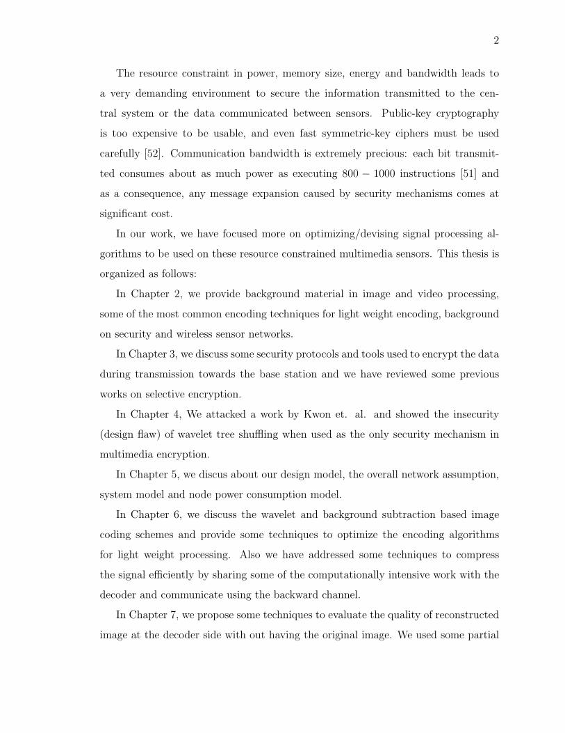
The resource constraint in power, memory size, energy and bandwidth leads to

a very demanding environment to secure the information transmitted to the cen-

tral system or the data communicated between sensors. Public-key cryptography

is too expensive to be usable, and even fast symmetric-key ciphers must be used

carefully [52]. Communication bandwidth is extremely precious: each bit transmit-

ted consumes about as much power as executing 800 − 1000 instructions [51] and

as a consequence, any message expansion caused by security mechanisms comes at

significant cost.

In our work, we have focused more on optimizing/devising signal processing al-

gorithms to be used on these resource constrained multimedia sensors. This thesis is

organized as follows:

In Chapter 2, we provide background material in image and video processing,

some of the most common encoding techniques for light weight encoding, background

on security and wireless sensor networks.

In Chapter 3, we discuss some security protocols and tools used to encrypt the data

during transmission towards the base station and we have reviewed some previous

works on selective encryption.

In Chapter 4, We attacked a work by Kwon et. al. and showed the insecurity

(design flaw) of wavelet tree shuffling when used as the only security mechanism in

multimedia encryption.

In Chapter 5, we discus about our design model, the overall network assumption,

system model and node power consumption model.

In Chapter 6, we discuss the wavelet and background subtraction based image

coding schemes and provide some techniques to optimize the encoding algorithms

for light weight processing. Also we have addressed some techniques to compress

the signal efficiently by sharing some of the computationally intensive work with the

decoder and communicate using the backward channel.

In Chapter 7, we propose some techniques to evaluate the quality of reconstructed

image at the decoder side with out having the original image. We used some partial

3

information about the original image sent along with the data as a side information

to compare the quality of the reconstructed image.

In Chapter 8, we describe the over all design of the decoder and the decoding

process. We also propose a block matching algorithm technique to predict position

vectors and give the information back to the encoder to reduce computation.

In Chapter 9 we conclude and discuss future work.

4

2. BACKGROUND MATERIAL

2.1 Image Compression - Using Wavelets

Images require substantial storage and transmission resources, thus image com-

pression is advantageous to reduce these requirements. This chapter covers some

background of wavelet analysis, data compression and how wavelets have been and

can be used for image compression.

2.1.1 Image/Video Compression

Image data by its nature is multidimensional and tends to take up significant

space (storage), computations (during its processing, such as in compression and

encryption) and transmission time and bandwidth. For example, two hours of video,

in HDTV resolution

2× 60× 60× 30× 1920× 1080× 3 = 1.22terabytes.

There are several constraints for transmitting the multimedia data in raw format,

such as transmission time and costs (ISPs charge per data amount, whereas phone

companies charge per time unit), limited hardware resources such as memory, CPU

etc (PDA, Cell phone, wireless sensors etc). Compressing an image is significantly

different than compressing raw data. Thus, general purpose compression programs are

not optimal when they are applied to compress a multimedia data since multimedia

data possess statistical properties which can be exploited by encoders specifically

designed for them. Also, the human visual system does not rely on quantitative

analysis of individual pixel values when interpreting an image - an observer searches

for distinct features and mentally combines them into recognizable groupings. In this

5

process certain information is relatively less important than other and some of the

finer details in the image can be sacrificed to save more bandwidth and storage space.

The fundamental task of image compression is to reduce the amount of data

required to represent an image. This is done by transforming and removing image

data redundancies mathematically; this is accomplished by transforming the data to

a statistically uncorrelated set. The two major categories of compression algorithms

are:

Lossless compression algorithms In this case the original data is reconstructed

perfectly. Theoretical limits exist concerning maximal compression perfor-

mance. Practical compression ratios are less than 10 : 1 (for still images).

Lossy compression algorithms In this case the the decompression results in an

approximation of the original image. Maximal compression rate is a function

of reconstruction quality, and practical compression ratios can be greater than

10 : 1 (for still images).

2.1.2 Wavelet Coding

A mathematical transformation is applied to signals to obtain further information

from that signal that is not readily available in the raw signal. Most of the signals

in practice are TIME-DOMAIN signals in their raw format. That is, whatever that

signal is measured it is a function of time. When we plot a time-domain signal,

we obtain a time-amplitude representation of the signal. For most signal processing

related applications, this representation is not always the best representation of the

signal. In many cases, the most distinguished information is hidden in the frequency

content of the signal. The frequency spectrum of a signal is basically the frequency

components (spectral components) of that signal and it shows what frequencies exist

in the signal.

We can measure the frequency content of a signal by applying mathematical

transform to the time-domain signal. Some of the mathematical transforms that

6

are used Fourier Transform (FT), Discrete Cosine Transform (DCT), Radon Trans-

form, Wavelet Transform, etc. If the Fourier transform of a signal in the time domain

is taken, we obtain the frequency-amplitude representation of that signal.

The frequency information of a signal is needed, because often, information that

cannot be readily seen in the time-domain can be seen in the frequency domain.

In electrical engineering, the Fourier transform is one of the most common and

widely used mathematical transformation techniques to convert the signal from time

domain to frequency domain.

For any periodic signal f(t), its Fourier transform is:

F (ω) =

∫ ∞

−∞f(t)e−jωtdt

The Fourier transform gives the frequency information of the signal, which means

that it provides how much of each frequency component exists in the signal, but it

does not tell us when, in time, these frequency components exist. Signals whose

frequency content do not change in time are called stationary signals [47]. In other

words, the frequency content of stationary signals do not change in time. In this

case, one does not need to know at what times frequency components exist, since all

frequency components exist at all times.

When the signal is a non-stationary signal, or when the time localization of the

spectral components are needed, a transform giving the Time-Frequency Representa-

tion of the signal is needed.

The wavelet transform is a transform of this type. It provides the time-frequency

representation.1 Often, a particular spectral component occurring at any instant can

be of particular interest. In these cases it may be very beneficial to know the time

intervals these particular spectral components occur. For example, the latency of

an event-related potential is of particular interest (the response to a specific trigger

or event), and one might be interested in the amount of time between the onset of

the trigger (stimulus) and the response. So we need a transform that is capable of

1There are other transforms which give this information, such as short time Fourier transform,Wigner distributions, etc.

7

providing the time and frequency information simultaneously, hence giving the time

frequency representation of the signal.

Mutiresolution Analysis and the Discrete Wavelet Transform

Like transform coding, wavelet coding is based on the premise that using a linear

transform, here a wavelet transform, will result in transform coefficients that can be

stored more efficiently than the pixels themselves. Due to the fact that wavelets are

computationally efficient and that the wavelet basis functions are limited in duration,

subdivision of the original image is unnecessary. Wavelet coding typically produces a

more efficient compression than Discrete Cosine Transform (DCT) based systems, the

blocking artifacts (characteristic of DCT-based systems at high compression ratios)

are not present in wavelet reconstructions The choice of the wavelet to use, greatly

affects the compression efficiency. For our work, we want a lightweight encoding, so

we have decided to use Haar wavelets, this is described in greater detail in Section

6.2.

2.2 Background Subtraction Method for Detecting Foreground Objects

Background subtraction is a widely used approach for detecting moving objects

from a static camera by differencing the current frame and a reference frame. The

result highly depends on how the reference image (modeled background) represent

the static scene (the scene with no moving object) of the camera view. So a good

model for estimating the background is necessary for optimal result.

2.2.1 Background Model - Estimating Good Background

Several methods of performing background subtraction have been proposed in

literature. These methods attempt to estimate the background model from the tem-

poral sequence of the frames. Each of these methods have their benefits as well as

8

their limitations. In the following, we provide some of the common techniques that

are used.

2.2.2 The Most Common Approaches of Background Generation

The approaches towards background generation range from simple ones, aiming

to maximize speed and limiting the memory requirement to more sophisticated ap-

proaches aiming to achieve the highest possible accuracy.

Running Gaussian Average

Wren, et al. [40] has proposed to model the background independently at each

(i, j) pixel location. The model is based on ideally fitting a Gaussian Probability

Density Function (PDF ) on the last n pixels values. In order to avoid constructing

the PDF function from scratch at each new frame time, t, a running average is

computed instead as:

µt = αIt + (1− α)µt−1 (2.1)

where It, is the pixels current value and µt the previous average; α is an empirical

weight often chosen as a tradeoff between stability and quick update. The other

parameter of the Gaussian PDF, the standard deviation σt, can be computed similarly.

The advantage of the running average technique is its high computational speed and

low memory requirement. For each pixel, there exists two parameters (µt, σt) instead

of the buffer with the last n pixel values. The update rate of either µt and/or σt can

be set to less than that of the sample (frame) rate. However, the lower the update

rate of the background model, the less the system will be able to quickly respond to

the actual background dynamic.

9

Temporal Median Filter

Several [41, 42] have proposed using a median filter to model background of the

static scene from the last N frames (median value of the last N frames as the as

the background model). Cucchiara, et al. [42] and Lo and Velastin [41] argued that

a median value provides an adequate background model even if the N frames are

subsampled with respect to the original frame rate by a factor of ten. In addition,

Lo et. al. [42] proposed to compute the median on a special set of values containing

the last N sub-sampled frames and W times the last computed median value. This

combination increases the stability of the background model.

The main disadvantage of a median-based approach is that its computation re-

quires a buffer with the recent pixel values. Moreover, the median filter does not

accommodate for a rigorous statistical description and does not provide a deviation

measure for adapting the subtraction threshold.

Gaussian Mixture Model

In the Running Gaussian Average background modelling technique, the back-

ground was modeled by a single distribution in each pixel. But this leads to problems

when the background is not static and when there is foreground in the training data.

This can be partially addressed by introducing multiple distributions. The idea is

to model each surface by own distribution. This, using a number of Gaussian dis-

tribution is called Gaussian Mixture Model. For a greater discussion concerning the

Gaussian Mixture Model see [43].

There are other models which are even more computationally intensive and mem-

ory demanding but with high accuracy. Some of them include: Kernel Density Es-

timation (KDE), Sequential KD approximation, Cooccurence of image variations,

Eigenbackgrounds, etc [48,49].

10

2.3 Security

Wireless sensor networks may operate in a hostile environment, so security is

crucial to ensure the integrity and confidentiality of sensitive information [50]. To

achieve this, the network need to be well protected from intrusion and spoofing. The

biggest challenge in securing the network infrastructure is the constrained computa-

tion and communication capability of sensor nodes. It makes it suitable to consider

nonconventional encryption techniques [52].

2.3.1 Cryptography

In cryptography, encryption is the process of transforming information (plaintext)

using an algorithm to make it unreadable to only those possessing the secret key. The

output of the transformation is called ciphertext. Encryption and decryption [61].

Encryption and Decryption algorithms are referred to as cryptographic algorithms or

cryptosystems. Cryptanalysis refers to the breaking of a cryptosystem.

Cryptosystems can be categorized into two classes: Symmetric key encryption and

Asymmetric key encryption.

Symmetric Key Encryption

Symmetric key cryptosystems (also called conventional key cryptosystems) are

encryption algorithms that uses identical cryptographic keys for both encryption and

decryption. Both the encryption and decryption keys are related in that they may

be identical or there is a simple transformation to construct the decryption key from

the encryption key.

Symmetric key algorithms can be divided in to stream ciphers and block ciphers.

Stream ciphers encrypt the bytes of the message one at a time, and block ciphers

take a number of bytes and encrypt them as a single unit. A Block of 64 bits was

used for DES. Today the AES algorithm uses 128-bit blocks [70]. Some common ex-

11

amples of symmetric algorithms include Data Encryption Standard (DES), Advanced

Encryption Standard (AES), RC4, TDES, etc.

Public Key Cryptosystem

The term Public Key Cryptosystems are also referred to as Asymmetric Key

Cryptosystems. Unlike symmetric key algorithms, public key cryptosystem does not

require a secure exchange of one or more secret key between client and server (sender

and receiver). The way public key cryptography works is that one entity has the

private key and keeps it safe not letting anyone else know it, the corresponding public

key is made freely available. Both the keys are mathematically related in some way

to each other, but at a glance, they should seem perfectly random. This makes

cryptanalysis of the algorithm a much more difficult process.

Asymmetric ciphers usually are more computationally intensive than their sym-

metric counterparts. Common examples of asymmetric ciphers are RSA, Diffie-

Hellman algorithm and Elliptic Curve Cryptosystems (ECC).

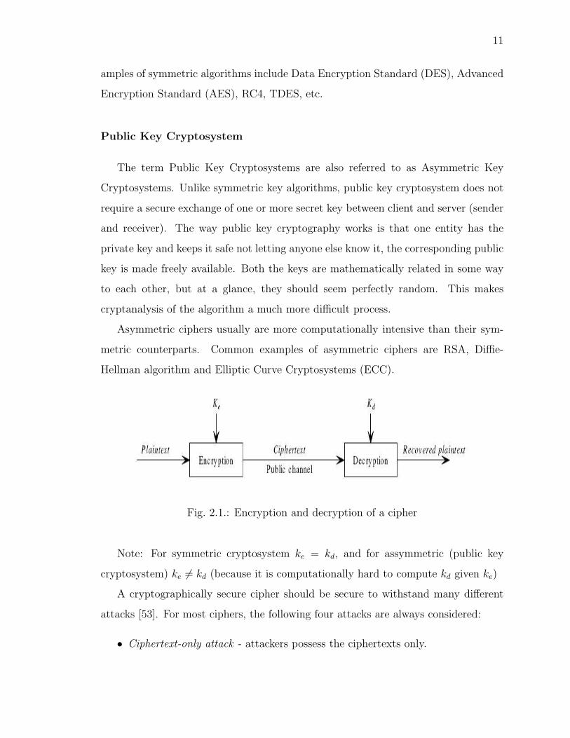
Fig. 2.1.: Encryption and decryption of a cipher

Note: For symmetric cryptosystem ke = kd, and for assymmetric (public key

cryptosystem) ke 6= kd (because it is computationally hard to compute kd given ke)

A cryptographically secure cipher should be secure to withstand many different

attacks [53]. For most ciphers, the following four attacks are always considered:

• Ciphertext-only attack - attackers possess the ciphertexts only.

12

• Known-plaintext attack - attackers possess some plaintexts and the correspond-

ing ciphertexts.

• Chosen-plaintext attack - attackers can select some plaintexts and get the cor-

responding ciphertexts.

• Chosen-ciphertext attack - attackers can select some ciphertexts and get the

corresponding plaintexts.

It is known that many image/video encryption schemes are not secure enough against

known/chosen-plaintext attacks. This will be described more in Chapter 4.

2.4 Multimedia Security

For digital rights management, confidential video conferencing, military and med-

ical imaging system, the multimedia data has to be encrypted during storage and

transmission through an open network.

2.4.1 Image/Video Encryption Scheme

The distinction between image encryption and video encryption is not prominent

since most encryption techniques proposed for image are extended to encrypt videos

with similar structures [54].

Some common image/video encryptions proposed in literature include:

• Almost all DCT based encryption schemes can be used to encrypt both image

and video datas [55] [54].

• Entropy encoding which is used widely both in image and video encoding. the

idea of making entropy code secret is proposed in different literatures as a se-

curity mechanism for image/video encryption. In [56, 57], the authors propose

secretely permuting huffman table to encrypt the input image/video stream.

13

In [58] also randomly flipping the last bit of each codeword to adaptively change

the Huffman table is proposed to encrypt image/video data.

• Wavelet based encryption has been suggested by many. In [59], selective bit

scrambling, block shuffling, and block rotation is proposed to encrypt image/video

wavelet compressed streams.

The existing or standard encryption algorithms are sometimes too intensive to

be applied for encrypting multimedia data in resource starved devices like cellphone,

PDA and wireless sensors. So another scheme called Selective Encryption is proposed

[13,72].

2.5 Selective Encryption

Selective encryption is a method of selectively concealing portions of a compressed

multimedia bitstream while leaving the remaining portions of the stream unchanged

[13]. This technique is widely adopted to encrypt multimedia data in resource starved

devices, and aims to achieve a better tradeoff between the encryption load and the

security level.

Related works and some review on selective encryption is discussed in Chapter

4. In that chapter we provide analysis concerning the insecurity of certain selective

encryption schemes. Specifically we attack a selective encryption scheme that is based

on shuffling spatial orientation trees of a wavelet based transform data structure.

14

3. SELECTIVE ENCRYPTION

3.1 Introduction

Internet multimedia applications has become extremely popular. Valuable multi-

media content such as digital images and video, are vulnerable to unauthorized access

while in storage as well as during a transmission over a network. Streaming of secure

images/real-time video in the presence of constraints, such as bandwidth, delay, com-

putational complexity and channel reliability is one of the most challenging problems.

For example, a 512× 512 color image at 24 bits/pixel would require 6.3Mbits. While

the bandwidth issue can be resolved using compression, securing multimedia data

still remains a big challenge, especially in light of the diversity of devices (in terms of

resource availability) that will transmit and receive the content.

Traditional image and video content protection schemes are fully layered, the

whole content is first compressed, and then the compressed stream is encrypted using

a standard cryptographic technique (such as TDES, AES, . . . ) [16]. However, the

requirement for high transmission rate with limited bandwidth makes this traditional

technique inadequate. In the fully layered scheme compression and encryption are two

different (disjoint) processes. The multimedia content is processed as a classical text

assuming that all the bits in the plaintext are equally important. But with constrained

resources (in real-time networking, high definition delivery, low power, low memory

and computational capability) this scheme is inefficient. Thus techniques for securing

multimedia data requiring less complexity and less adverse effect on the compression

without compromising the security of the data is required. One such technique is to

use selective encryption [4,60]. Selective encryption is an encryption technique based

on combining the encryption and compression process, that will reduce computational

15

complexity as well as bandwidth utilization, by encrypting only the “essential parts

of the image”. In Section 3.3, we briefly discuss some selective encryption techniques.

This work focuses on the analysis of a selective encryption technique that is based

on the permutation (shuffling) of wavelet trees, a technique that was suggested by

Kwon, et. al. [5] to be used as the sole base of providing privacy. Here we demonstrate

that as the sole cryptographic primitive it is weak.

3.2 Wavelet Based Compression Techniques

Over the past several years, the wavelet transform has gained widespread accep-

tance in image compression research. Since there is no need to divide the image into

macro blocks (no need to block the input image), wavelet based coding at higher

compression avoids blocking artifacts. Wavelet transform can decompose a signal in

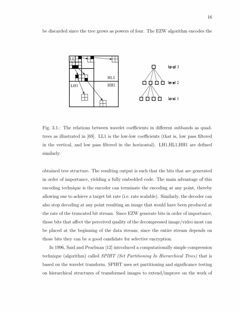
to different subbands. There are many compression techniques that use the wavelet

transform, including JPEG-2000, EZW [14] and SPIHT [12]. We now briefly discuss

EZW and SPIHT.

In 1993, Shapiro [14] presented an algorithm for entropy encoding called Embedded

Zerotree Wavelet (EZW) algorithm. After applying the wavelet transform, the coef-

ficients can be represented using trees because of the subsampling that is performed

in the transform. A coefficient in a low subband can be thought of as having four

descendants in the next higher subband (see Figure 1). The four descendants each

have four descendants in the next higher subband and we see a quad-tree structure

emerges and every root has four leafs. A zerotree is a quad-tree of which all nodes are

equal to or smaller than the root. The zero tree structure is based on the hypothesis

that if a wavelet coefficient at a coarse scale is insignificant with respect to a given

threshold T, then all wavelet coefficients of the same orientation in the same spatial

location at finer scales are likely to be insignificant with respect to T. The idea is

to define a tree of zero symbols that start at a root that is also zero and label as

end-of-block. Many insignificant coefficients at higher subbands (finer resolution) can

16

be discarded since the tree grows as powers of four. The EZW algorithm encodes the

Fig. 3.1.: The relations between wavelet coefficients in different subbands as quad-

trees as illustrated in [69]. LL1 is the low-low coefficients (that is, low pass filtered

in the vertical, and low pass filtered in the horizontal). LH1,HL1,HH1 are defined

similarly.

obtained tree structure. The resulting output is such that the bits that are generated

in order of importance, yielding a fully embedded code. The main advantage of this

encoding technique is the encoder can terminate the encoding at any point, thereby

allowing one to achieve a target bit rate (i.e. rate scalable). Similarly, the decoder can

also stop decoding at any point resulting an image that would have been produced at

the rate of the truncated bit stream. Since EZW generate bits in order of importance,

those bits that affect the perceived quality of the decompressed image/video most can

be placed at the beginning of the data stream; since the entire stream depends on

those bits they can be a good candidate for selective encryption.

In 1996, Said and Pearlman [12] introduced a computationally simple compression

technique (algorithm) called SPIHT (Set Partitioning In Hierarchical Trees) that is

based on the wavelet transform. SPIHT uses set partitioning and significance testing

on hierarchical structures of transformed images to extend/improve on the work of

17

Shapiro [14]. SPIHT is also a good candidate to be used in a selective encryption

scheme.

3.3 Prior Work on Selective Encryption

Selective encryption has been suggested and adopted as a basic idea for encryp-

tion of digital images and videos, aiming to achieve a better trade off between the

encryption load and the security level. Selective encryption is a method of selectively

concealing portions of a compressed multimedia bitstream while leaving the remaining

portions of the stream unchanged.

There are a number of selective encryption techniques. Here we briefly discuss

only a few schemes. For more details and a more thorough discussion we suggest the

reader look at [7, 60].

In 2002, Podesser, Schmidt and Uhl [10] applied the following technique. They

proposed a selective bitplane encryption using AES. They conducted a series of ex-

periments on 8-bit grayscale images, and observed the following: (1) encrypting only

the MSB is not secure; a replacement attack is possible, (2) encrypting the first two

MSBs gives hard visual degradation, and (3) encrypting three bitplanes gives very

hard visual degradation.

Zeng and Lei [71] proposed a selective encryption scheme in the frequency domain

(wavelet domain). The general scheme consists of selective scrambling of coefficients

by using different primitives (selective bit scrambling, block shuffling, and/or rota-

tion). The input video frames are transformed using wavelet transform and each

subband represents selected spatial frequency information of the input video frame.

The authors propose two ways to scramble the coefficients. In their first suggestion,

they observed that some bits of the transform coefficients have high entropy and can

thus be encrypted without greatly affecting compressibility. In their second sugges-

tion, the authors observed that shuffling the arrangement of coefficients in a transform

coefficient map can provide effective security without destroying compressibility, as

18

long as the shuffling does not destroy the low-entropy aspects of the map relied upon

by the bitstream coder. To increase security, the authors suggested block shuffling.

Each subband is divided into a number of blocks of equal size (the size of the block

can vary for different subbands) and within each subband, blocks of coefficients will

be shuffled according to a shuffling table generated using a key.

Kwon, Lee, Kim, Jin, and Ko [5] described a scheme which involves shuffling of

spatial orientation trees (SOT) to secure multimedia data. The authors mentioned the

deficiency of traditional block shuffling technique and proposed wavelet tree shuffling

as an alternate security mechanism as part of the security architecture for multimedia

digital rights management. The authors proposed a 4-level wavelet transform. Ac-

cording to Shapiro’s [14] algorithm, this will result in 13 sub-bands, and the wavelet

coefficients are grouped according to wavelet trees.

In 2005, Salama and King [13] proposed a joint encryption-compression technique

(Selective Encryption) for securing multimedia data based on the EZW compression

scheme. Their approach is selectively encrypting those bits for which the entire bit

stream depends. Through a serious of experiments/simulations, the authors found

that encrypting the leading 256 bits of a 512 × 512 image will provide sufficient se-

curity. In their scheme, first the image will be transformed using discrete wavelet

transform, apply EZW, and then entropy encoded before it is encrypted using the

proposed Selective Encryption technique. The authors developed a security analysis

of the proposed joint compression-encryption technique, and demonstrated an attack

called Database Attack. In this attack, an adversary (unintended receiver) can inter-

cept the encrypted signal and attempt to replace the encrypted portion of the data

stream by another portion that he/she would generate. For the attack to be success-

ful, the interceptor would need a selective database (small enough for computations

to be feasible and large enough to include all possible target images), that contains

at least one of the possible images that can be transmitted. The attacker then per-

forms a brute force attack by encoding all images in the database and comparing the

unprotected part of the stream with the corresponding part of the compressed images

19

from the database. If there is a match, the attacker can replace one stream with

another. As a countermeasure to this attack, the authors propose Randomly shuf-

fling the SOT prior to encoding, shuffling the SOT (spatial orientation trees) after

wavelet transform. This will frustrate brute force database attack without affecting

the compression performance.

In 2006, Wu and Mao [8] proposed a shuffling technique as part of their selective

encryption architecture. The authors use the MPEG-4 fine granularity scalability

(FGS) functionality provided by the MPEG-4 streaming video profile [6] to illustrate

their concept and approach. A video is first encoded into two layers, a base layer that

provides a basic quality level at a low bit rate and an enhancement layer that provides

successive refinement. The enhancement layer is encoded bitplane by bitplane from

the most significant bitplane to the least significant one to achieve fine granularity

scalability. The authors propose an intra bit plan shuffling on each bit plane of n-bits

according to a set of cryptographically secure shuffle tables and using a run-EOP

approach. In addition to bit-plane shuffling, the authors also proposed randomly

flipping the sign bit si of each coefficient according to a pseudo-random bit bi from a

one-time pad, i.e., the sign remains the same when bi = 0 and changes when bi = 1.

20

4. ATTACKING WAVELET TREE SHUFFLING

ENCRYPTION SCHEME

In this chapter, we are analyzing shuffling of the wavelet trees (SOT’s) as if it were

the only mechanism used for encryption. First we describe what a generic wavelet

tree shuffling encryption scheme would be, as discussed in [5].

4.1 A Generic Framework of a Wavelet Tree Shuffling Encryption Scheme

Here we outline the construction of an encryption scheme which is based on the

use of permuting the trees which are produced by the wavelet transform. This scheme

was suggested by Kwon et. al. in [5].

Suppose the image I is of size M ×N . Then I can be represented as

I =

m0,0 · · · m0,N−1

.... . .

...

mM−1,0 · · · mM−1,N−1

M×N

(4.1)

where mi,j is the i, j pixel of I.

For a level L of wavelet decomposition the number of SOT’s (spatial orientation tree)

is

T =M ·N

22L(4.2)

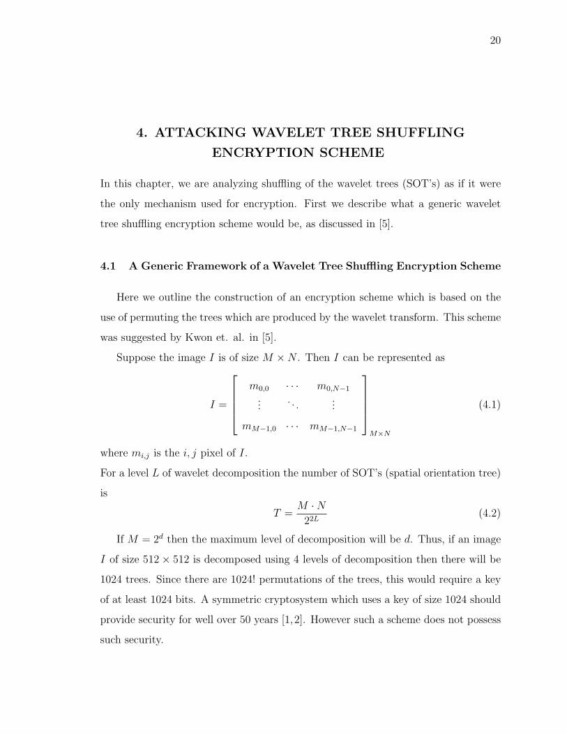
If M = 2d then the maximum level of decomposition will be d. Thus, if an image

I of size 512× 512 is decomposed using 4 levels of decomposition then there will be

1024 trees. Since there are 1024! permutations of the trees, this would require a key

of at least 1024 bits. A symmetric cryptosystem which uses a key of size 1024 should

provide security for well over 50 years [1,2]. However such a scheme does not possess

such security.

21

Encryption:

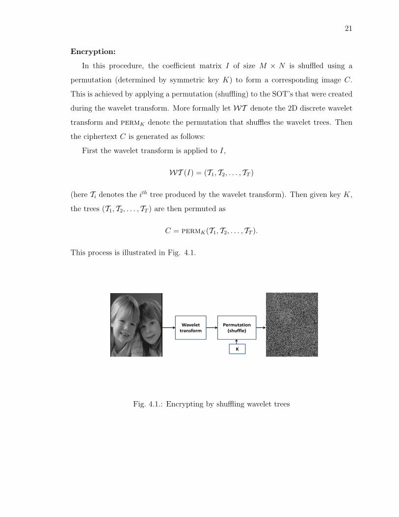
In this procedure, the coefficient matrix I of size M × N is shuffled using a

permutation (determined by symmetric key K) to form a corresponding image C.

This is achieved by applying a permutation (shuffling) to the SOT’s that were created

during the wavelet transform. More formally let WT denote the 2D discrete wavelet

transform and permK denote the permutation that shuffles the wavelet trees. Then

the ciphertext C is generated as follows:

First the wavelet transform is applied to I,

WT (I) = (T1, T2, . . . , TT )

(here Ti denotes the ith tree produced by the wavelet transform). Then given key K,

the trees (T1, T2, . . . , TT ) are then permuted as

C = permK(T1, T2, . . . , TT ).

This process is illustrated in Fig. 4.1.

Wavelet transform

Permutation(shuffle)

K

Fig. 4.1.: Encrypting by shuffling wavelet trees

22

Decryption:

Given the ciphertext C, the image I is then reconstructed as follows. First the

inverse of the permutation (that was induced by key K) is applied. Thus

(T1, T2, . . . , TT ) = perm−1K (C).

Then the IWT (inverse wavelet transform) is applied. The result is

I = IWT (T1, T2, . . . , TT ).

4.2 Attacking a Wavelet Tree Shuffling Encryption Scheme

In this work, we are analyzing shuffling of the wavelet trees (SOT’s) as if it were

the only mechanism used for encryption [5].

Norcern and Uhl [9] also discussed the insecurity of a system (in terms of com-

pression performance) that was based on randomly permuting wavelet-subbands in-

corporated in the JPEG2000 or the SPIHT coder proposed by Uehara et. al. in [17].

Their work differs from ours in the sense that they were attacking a scheme that

was randomly permuting the coefficients of wavelet subbands, while our attack is

on encryption schemes that are shuffling the tree structure created after the wavelet

transform.

The basis of our attack will be a chosen plaintext attack, in particular a lunch

time attack We will assume that the attacker has temporary possession of the en-

cryption machine and can feed the machine selected plaintext and will receive the

corresponding ciphertext. From this lunch time attack the adversary will be able to

determine the permutation (encryption) key.

First consider an image of size M×N and suppose it is transformed in to wavelet

coefficients using the L-level discrete wavelet transform (DWT). With an L-level

decomposition, we have 3L+ 1 frequency bands. In Fig 4.4, when L = 4, the lowest

frequency subband is located in the top left (i.e., the LL4 subband, and the highest

frequency subband is at the bottom right (i.e., the HH1 subband). The relation

23

between this frequency bands can be seen as a parent-child relationship [14]. Thus,

for an image of size M×N with L-level of decomposition, in total we will have M2L · N2L

trees. After constructing wavelet trees, a secret key K is used to randomly shuffle the

trees.

Clearly if an attacker can guess the size of the image and the number of levels of

decomposition, then shuffling of the wavelet trees (SOT’s) is vulnerable to the lunch

time attack. A simple scenario of a lunch time attack: a legitimate user s away from

the desk (computer) without locking their computer/machine, the attackers can use

a chosen plaintext attack. A chosen plaintext attack can be launched by any party

(adversary) who can access the machine while the user is absent. For the attack to be

successful, the adversary needs to have access for the encryption machine. Once the

adversary has access to the encryption machine, he/she can choose a series of chosen

plaintexts and feed them to the encryption machine as shown in Fig. 4.5. Thus if

Ij denotes a chosen plaintext, and if we denote the wavelet tree shuffling encryption

scheme (as illustrated in Fig 4.1) by E(Ij, K) where K is the key, then the adversary

will generate chosen plaintexts

E(I1, K), E(I2, K), . . . , E(Ir, K).

The adversary can use these to determine the image size and the level of decomposi-

tion. Thus we will assume that the adversary knows these parameters.

In [5], Kwon et. al. proposed the shuffling of wavelet trees of a wavelet coefficient

which undergoes 4-levels of wavelet decomposition as part of their security architec-

ture for digital rights management. For an image of size 512× 512 which undergoes

4-levels of wavelet decomposition, there will be 1024 trees according to Equation 4.2 .

And shuffling of these trees using a randomized shuffling key (shuffling matrix) should

provide a security of 1024 bit key size.

Though Kwon et. al. [5] were using a level L = 4 of decomposition for an image

of size 512 × 512, we will provide an analysis/experiments based on image size of

256×256. Only a slight modification of our experiments would have to be constructed

24

to attack an image of size 512×512. The following table demonstrates the relationship

between the level of decomposition and the number of trees.

Table 4.1: Relationship between no. of decomp. and no. of trees for an image of size

256× 256

No. of decomp. No. of trees

3 1024

4 256

5 64

6 8

7 4

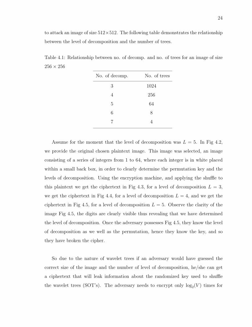
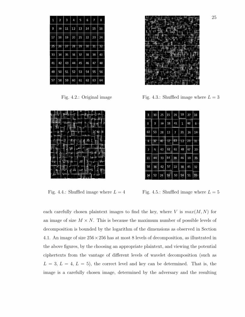
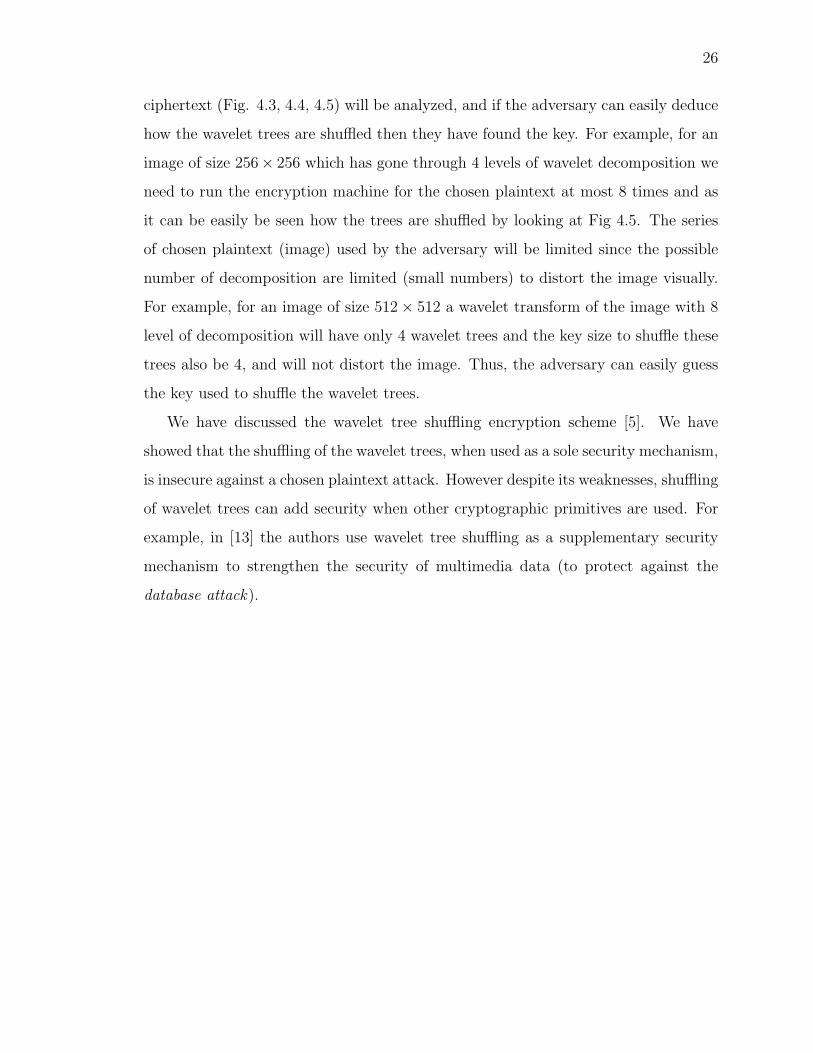
Assume for the moment that the level of decomposition was L = 5. In Fig 4.2,

we provide the original chosen plaintext image. This image was selected, an image

consisting of a series of integers from 1 to 64, where each integer is in white placed

within a small back box, in order to clearly determine the permutation key and the

levels of decomposition. Using the encryption machine, and applying the shuffle to

this plaintext we get the ciphertext in Fig 4.3, for a level of decomposition L = 3,

we get the ciphertext in Fig 4.4, for a level of decomposition L = 4, and we get the

ciphertext in Fig 4.5, for a level of decomposition L = 5. Observe the clarity of the

image Fig 4.5, the digits are clearly visible thus revealing that we have determined

the level of decomposition. Once the adversary possesses Fig 4.5, they know the level

of decomposition as we well as the permutation, hence they know the key, and so

they have broken the cipher.

So due to the nature of wavelet trees if an adversary would have guessed the

correct size of the image and the number of level of decomposition, he/she can get

a ciphertext that will leak information about the randomized key used to shuffle

the wavelet trees (SOT’s). The adversary needs to encrypt only log2(V ) times for

25

Fig. 4.2.: Original image Fig. 4.3.: Shuffled image where L = 3

Fig. 4.4.: Shuffled image where L = 4 Fig. 4.5.: Shuffled image where L = 5

each carefully chosen plaintext images to find the key, where V is max(M,N) for

an image of size M ×N . This is because the maximum number of possible levels of

decomposition is bounded by the logarithm of the dimensions as observed in Section

4.1. An image of size 256×256 has at most 8 levels of decomposition, as illustrated in

the above figures, by the choosing an appropriate plaintext, and viewing the potential

ciphertexts from the vantage of different levels of wavelet decomposition (such as

L = 3, L = 4, L = 5), the correct level and key can be determined. That is, the

image is a carefully chosen image, determined by the adversary and the resulting

26

ciphertext (Fig. 4.3, 4.4, 4.5) will be analyzed, and if the adversary can easily deduce

how the wavelet trees are shuffled then they have found the key. For example, for an

image of size 256× 256 which has gone through 4 levels of wavelet decomposition we

need to run the encryption machine for the chosen plaintext at most 8 times and as

it can be easily be seen how the trees are shuffled by looking at Fig 4.5. The series

of chosen plaintext (image) used by the adversary will be limited since the possible

number of decomposition are limited (small numbers) to distort the image visually.

For example, for an image of size 512× 512 a wavelet transform of the image with 8

level of decomposition will have only 4 wavelet trees and the key size to shuffle these

trees also be 4, and will not distort the image. Thus, the adversary can easily guess

the key used to shuffle the wavelet trees.

We have discussed the wavelet tree shuffling encryption scheme [5]. We have

showed that the shuffling of the wavelet trees, when used as a sole security mechanism,

is insecure against a chosen plaintext attack. However despite its weaknesses, shuffling

of wavelet trees can add security when other cryptographic primitives are used. For

example, in [13] the authors use wavelet tree shuffling as a supplementary security

mechanism to strengthen the security of multimedia data (to protect against the

database attack).

27

5. DESIGN MODEL

5.1 Introduction - Design Summary

Signal processing applications in wireless sensor networks need to consider re-

source constraints. With high energy cost for wireless communications, application

algorithms should be designed to reduce communication cost. Sensor readings are

highly correlated spatially and temporally. Effective exploitation of these correla-

tions can reduce data communication cost significantly. In most sensor applications,

events are not occurring in a consecutive manner. Therefore, it is a waste of energy

to keep nodes active for periods when no events are happening.

In our work, we investigated energy efficiency and power awareness in wireless

sensor networks. Although for efficient energy operation of sensors, both the net-

working protocol and signal processing algorithms have to be optimized. Our work

concerns devising signal processing algorithms and modifying some of the existing

signal processing algorithms to fit the application (to be feasible to be used under

resource constraint), as well as support energy efficient operations in wireless sensor

networks. We constructed an overall design of how the encoder and decoder will inter-

act. Lastly, we have verified the effectiveness and energy efficiency of our algorithms

via simulations.

5.2 Design Goal

Compression of Sensor Readings

In our work we will use

1. Integer based Haar wavelet transform and run-length based coding of sensor

readings without taking into account spatial correlation.

28

2. We have also considered Background Subtraction. This is proposed for lightweight

encoding of sensor readings, for situations where images are correlated tempo-

rally.

3. We construct an encoder/decoder design that switches compression mode be-

tween using Discrete Wavelet Transform (DWT) and using Background Sub-

traction based on feedback/directions from the decoder.

Exploiting Correlation of Sensor Readings

We intend to construct an encoding scheme that reverses the traditional balance of

complex encoder and simple decoder is proposed. It uses Block Matching Algorithm

(BMA) to quantify spatial correlation of readings of proximate sensors at the decoder

side and send the parameters using backward channel optimize the encoder. It has

recently been shown [34] that the traditional balance of complex encoder and sim-

ple decoder can be reversed within the framework of the so-called distributed source

coding, which exploits the source statistics at the decoder, and by shifting the com-

plexity at this end, allows the use of simple encoders. Clearly, such algorithms are

very promising for WMSNs and specially for networks of video sensors, where it may

not be feasible to use existing video encoders at the source node due to processing

and energy constraints. Inspired by this idea and a work by Delp et. al. [29], we have

designed a system that will shift some of the computationally intensive operations of

the encoder to the decoder side and use the backward channel to send parameters to

the encoder.

Because we will use a number of compression techniques our sensors need to

get feedback from the decoder concerning the quality of images. Consequently we

introduce a Reduced-Reference quality assessment method is proposed to measure

quality of the reconstructed image with out having the original image. It uses some

statistics about the original image as a side information to assess the quality of the

reconstructed image.

29

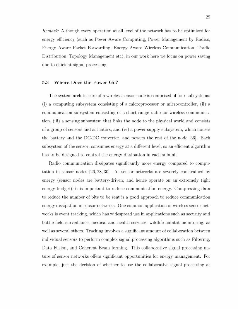
Remark: Although every operation at all level of the network has to be optimized for

energy efficiency (such as Power Aware Computing, Power Management by Radios,

Energy Aware Packet Forwarding, Energy Aware Wireless Communication, Traffic

Distribution, Topology Management etc), in our work here we focus on power saving

due to efficient signal processing.

5.3 Where Does the Power Go?

The system architecture of a wireless sensor node is comprised of four subsystems:

(i) a computing subsystem consisting of a microprocessor or microcontroller, (ii) a

communication subsystem consisting of a short range radio for wireless communica-

tion, (iii) a sensing subsystem that links the node to the physical world and consists

of a group of sensors and actuators, and (iv) a power supply subsystem, which houses

the battery and the DC-DC converter, and powers the rest of the node [36]. Each

subsystem of the sensor, consumes energy at a different level, so an efficient algorithm

has to be designed to control the energy dissipation in each subunit.

Radio communication dissipates significantly more energy compared to compu-

tation in sensor nodes [26, 28, 30]. As sensor networks are severely constrained by

energy (sensor nodes are battery-driven, and hence operate on an extremely tight

energy budget), it is important to reduce communication energy. Compressing data

to reduce the number of bits to be sent is a good approach to reduce communication

energy dissipation in sensor networks. One common application of wireless sensor net-

works is event tracking, which has widespread use in applications such as security and

battle field surveillance, medical and health services, wildlife habitat monitoring, as

well as several others. Tracking involves a significant amount of collaboration between

individual sensors to perform complex signal processing algorithms such as Filtering,

Data Fusion, and Coherent Beam forming. This collaborative signal processing na-

ture of sensor networks offers significant opportunities for energy management. For

example, just the decision of whether to use the collaborative signal processing at

30

the user end-point or somewhere inside the network has significant implication on

energy and lifetime, and our work, as described in Section 8.1.2, concerns exploiting

spatial correlation between neighborhood sensors at the base station side. We use

tracking/surveillance as our target application to motivate many of the techniques

presented in our research here. In general, sensor readings from near-by sensors are

correlated in space. Rather than straight data compression, spatial correlation can

be exploited to achieve improved data compression. The distributed source coding

problem of correlated sources has been studied extensively [53, 44, 25, 22].

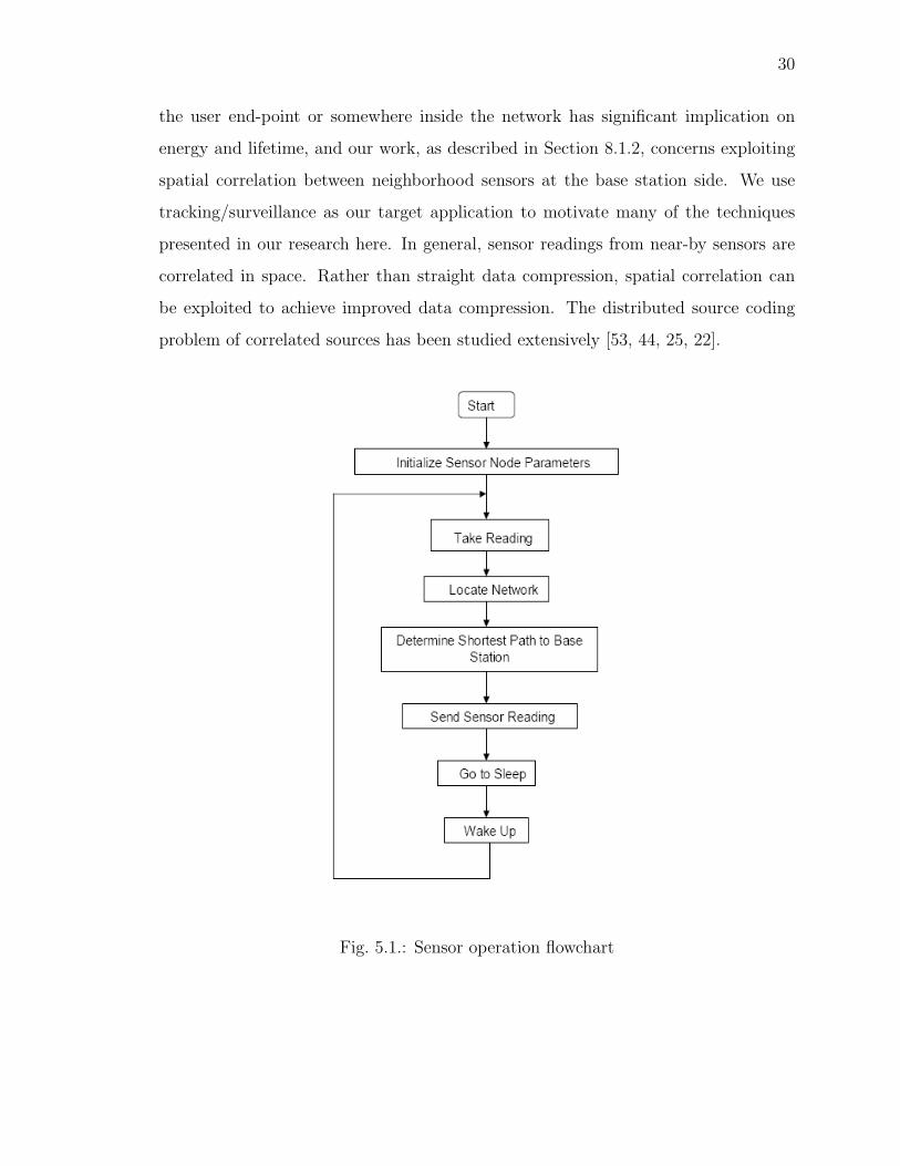
Fig. 5.1.: Sensor operation flowchart

31

5.4 Energy/Power Analysis of Sensor Nodes

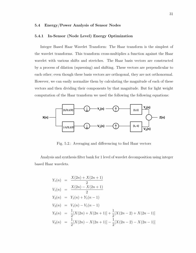
5.4.1 In-Sensor (Node Level) Energy Optimization

Integer Based Haar Wavelet Transform: The Haar transform is the simplest of

the wavelet transforms. This transform cross-multiplies a function against the Haar

wavelet with various shifts and stretches. The Haar basis vectors are constructed

by a process of dilation (squeezing) and shifting. These vectors are perpendicular to

each other; even though these basis vectors are orthogonal, they are not orthonormal.

However, we can easily normalize them by calculating the magnitude of each of these

vectors and then dividing their components by that magnitude. But for light weight

computation of the Haar transform we used the following the following equations:

Y1(n)

V1(n)

Y2(n)

V2(n)

Z(n)X(n)

{1/2,1/2}

{-1/2,1/2}

{1,1}

{1,-1}

Fig. 5.2.: Averaging and differencing to find Haar vectors

Analysis and synthesis filter bank for 1 level of wavelet decomposition using integer

based Haar wavelets.

Y1(n) =X(2n) +X(2n+ 1)

2

V1(n) =X(2n)−X(2n+ 1)

2

Y2(n) = Y1(n) + Y1(n− 1)

V2(n) = V1(n)− V1(n− 1)

Y2(n) =1

2[X(2n) +X(2n+ 1)] +

1

2[X(2n− 2) +X(2n− 1)]

V2(n) =1

2[X(2n)−X(2n+ 1)]− 1

2[X(2n− 2)−X(2n− 1)]

32

where X(n) is the original signal, Y1(n) and V1(n) are the decimated version of the

low-pass and high-pass coefficients respectively (analysis filter); and Y2(n) and V2(n)

are the interpolated version of the low-pass and high-pass coefficients respectively

(synthesis filter).

5.4.2 Network-Wide Energy Optimization

Traffic Distribution: One aspect of traffic forwarding is the choice of an energy

efficient multi-hop route between source and destination. Several approaches have

been proposed [37,38] which aim at selecting a path that minimizes the total energy

consumption. However, such a strategy does not always maximize the network lifetime

[39]. So although the shortest path towards the base station seems the best way, it has

to be carefully studied to distribute the traffic for more optimal packet forwarding.

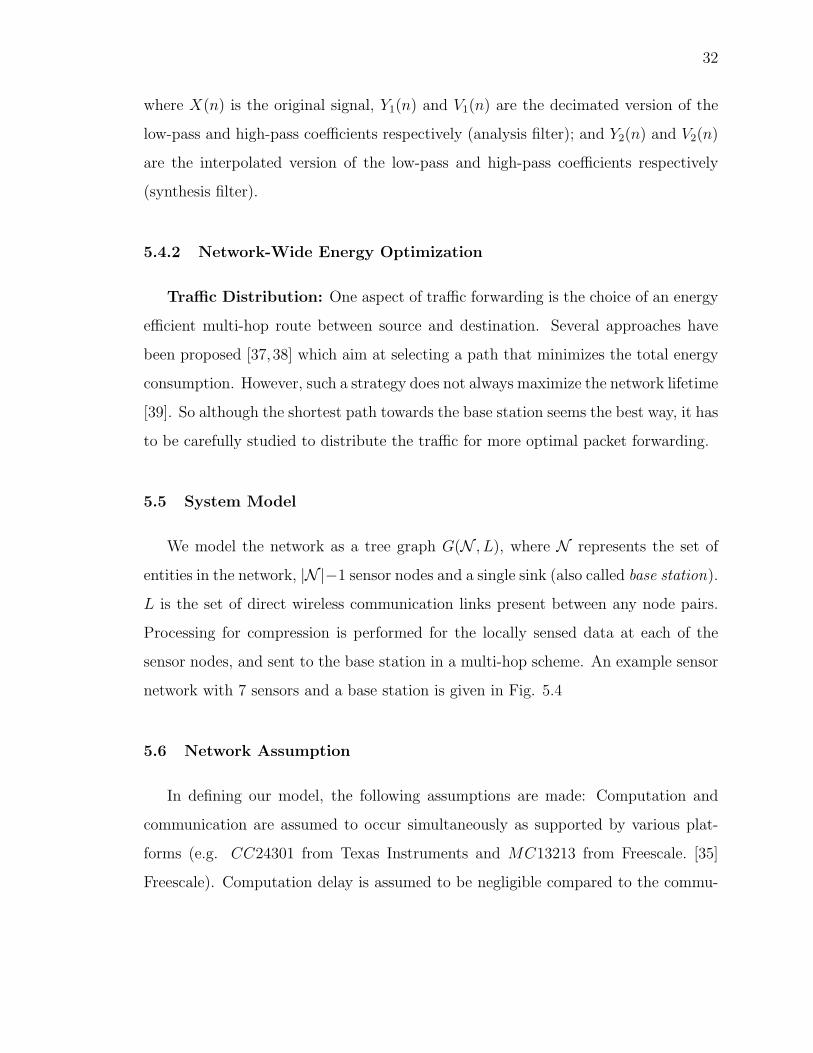
5.5 System Model

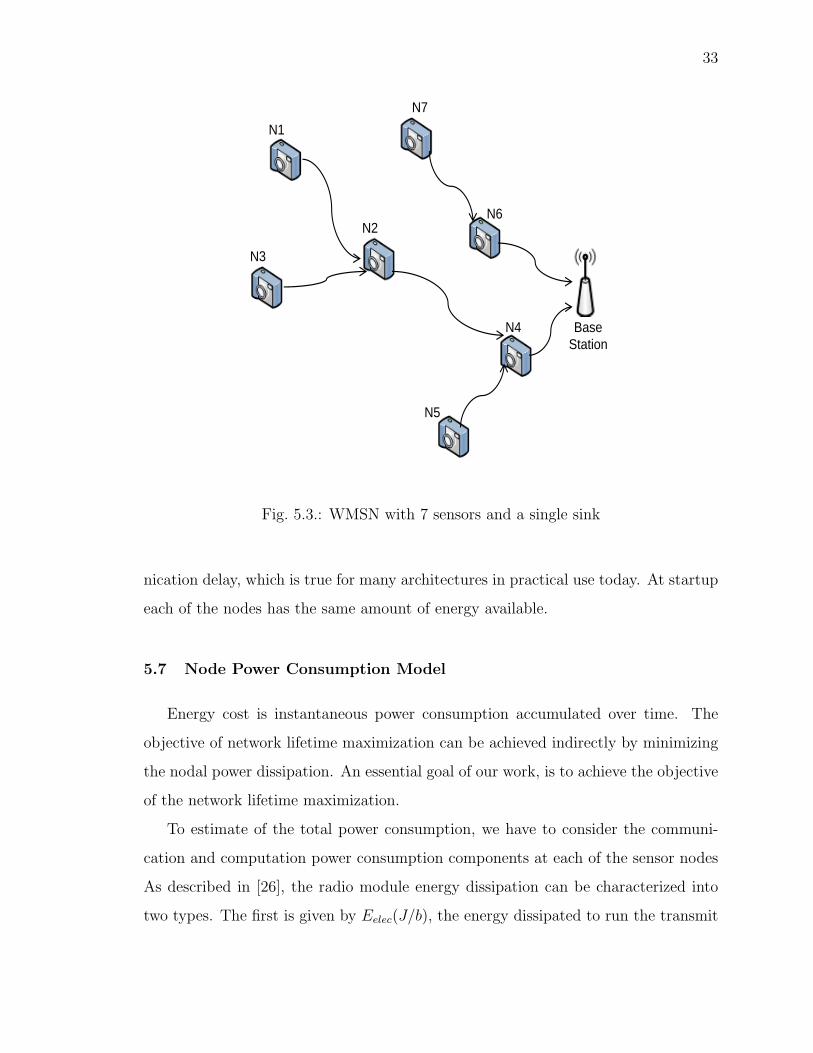
We model the network as a tree graph G(N , L), where N represents the set of

entities in the network, |N |−1 sensor nodes and a single sink (also called base station).

L is the set of direct wireless communication links present between any node pairs.

Processing for compression is performed for the locally sensed data at each of the

sensor nodes, and sent to the base station in a multi-hop scheme. An example sensor

network with 7 sensors and a base station is given in Fig. 5.4

5.6 Network Assumption

In defining our model, the following assumptions are made: Computation and

communication are assumed to occur simultaneously as supported by various plat-

forms (e.g. CC24301 from Texas Instruments and MC13213 from Freescale. [35]

Freescale). Computation delay is assumed to be negligible compared to the commu-

33

N1

N4

N5

N6N2

N7

N3

Base

Station

Fig. 5.3.: WMSN with 7 sensors and a single sink

nication delay, which is true for many architectures in practical use today. At startup

each of the nodes has the same amount of energy available.

5.7 Node Power Consumption Model

Energy cost is instantaneous power consumption accumulated over time. The

objective of network lifetime maximization can be achieved indirectly by minimizing

the nodal power dissipation. An essential goal of our work, is to achieve the objective

of the network lifetime maximization.

To estimate of the total power consumption, we have to consider the communi-

cation and computation power consumption components at each of the sensor nodes

As described in [26], the radio module energy dissipation can be characterized into

two types. The first is given by Eelec(J/b), the energy dissipated to run the transmit

34

or receive electronics and the second is given by εamp(J/b/m2), the energy dissipated

by the transmit power amplifier to achieve an acceptable Eb/No at the receiver. We

assume d2 energy loss for transmission between sensors (assuming the distances be-

tween sensors are relatively short) [27]. To transmit a k-bit packet a distance, d, the

energy dissipated is:

Etx(k, d) = Eelec · k + εamp · k · d2 (5.1)

and to receive the k − bit packet, the radio expends

Erx(k) = Eelec · k (5.2)

For µAmp wireless sensor, Eelec = 50nJ/b and εamp = 100pJ/b/m2 [26]. To prolong

the lifetime of the wireless sensor all aspects of the sensor system should be energy ef-

ficient. There should be efficient network protocol layer and efficient signal processing

algorithm. Our work fconcerns the energy dissipated at the radio and communication

module, in particular, local energy efficient signal processing.

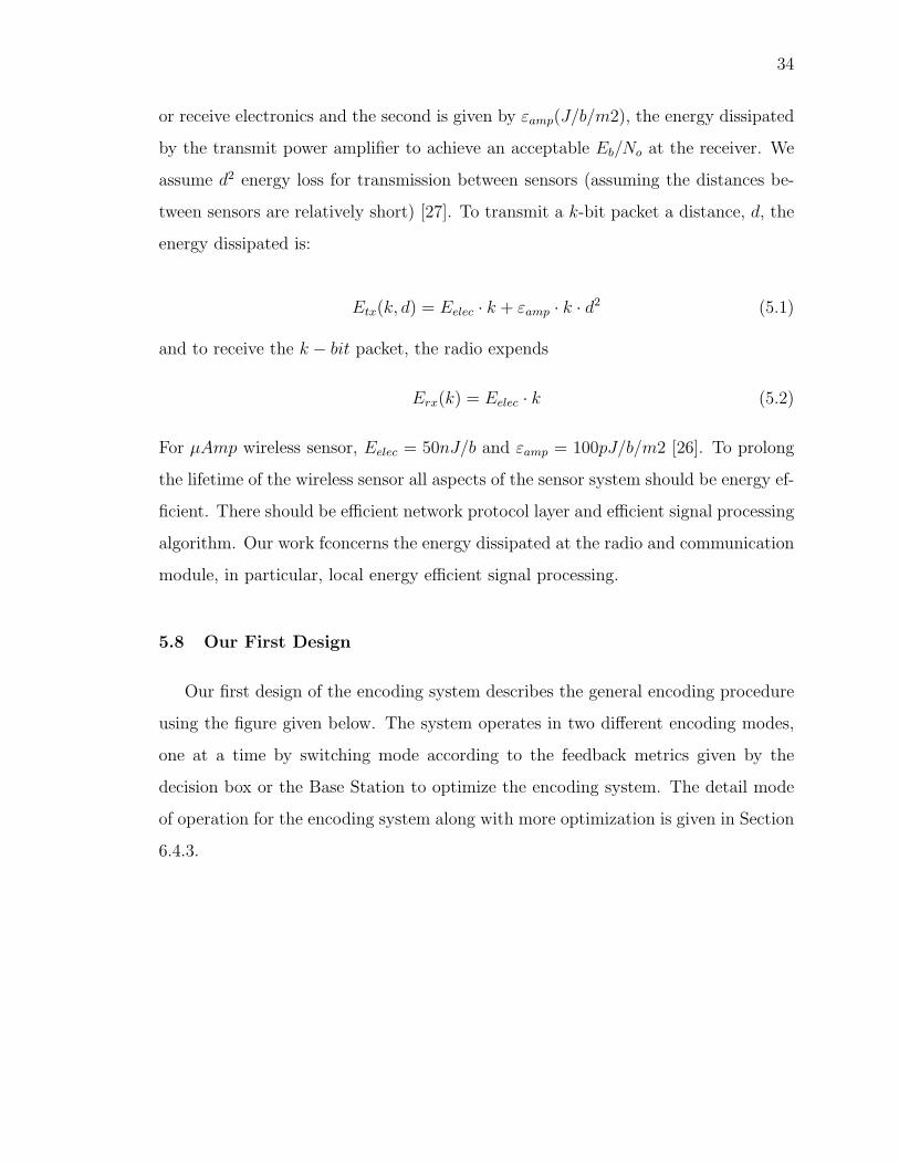
5.8 Our First Design

Our first design of the encoding system describes the general encoding procedure

using the figure given below. The system operates in two different encoding modes,

one at a time by switching mode according to the feedback metrics given by the

decision box or the Base Station to optimize the encoding system. The detail mode

of operation for the encoding system along with more optimization is given in Section

6.4.3.

35

Our First Encoder DesignOu s code es g• A scheme that switches compression mode between Discrete Wavelet

Transform (DWT) and Background Subtraction based on feedback from the decoder is proposeddecoder is proposed.

• This is achieved by using getting feedback from the decoder using the backward channel.

Background

Background model

Cache

Image

BackgroundExtraction

Region LevelThresholding

FGSuitable??

CodeBookExtraction Run Length

Encoding

Mode Packet Forwarded to the base station in a multi‐hop fashion

Wavelet Transform &Thresholding

Fig. 5.4.: A fist design of our encoder

36

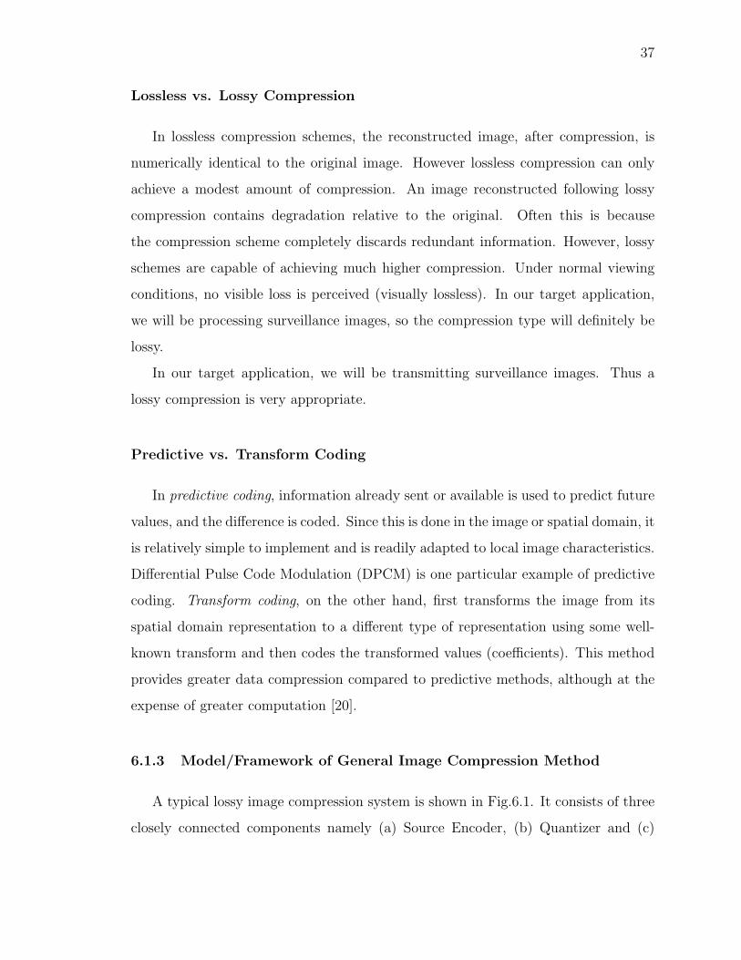
6. ENCODER

6.1 Introduction

For both archiving, as well as transmission through the network multimedia data

has to be compressed. The principal approach in image compression is the reduction

of the amount of image data(bits) while preserving information (image details).

6.1.1 Principles of Image Compression

A common characteristic of images is that the neighboring pixels are correlated

and thus hold redundant information. A mathematical operation can be performed

to determine the uncorrelated representations within the image. Two elementary

components of compression are redundancy reduction and irrelevancy reduction. Re-

dundancy reduction aims at removing duplication from the signal source image. Ir-

relevancy reduction omits parts of the signal that is not noticed by the signal receiver,

namely the Human Visual System (HVS). In general, three types of redundancy can

be identified: (a) Spatial Redundancy or correlation between neighboring pixel val-

ues, (b) Spectral Redundancy or correlation between different color planes or spectral

bands and (c) Temporal Redundancy or correlation between adjacent frames in a se-

quence of images specially in video applications. Image compression research aims at

reducing the number of bits needed to represent an image by removing the spatial

and spectral redundancies as much as possible.

6.1.2 Classification of Compression Technique

There are two ways that we can consider for classifying compression techniques-

lossless vs. lossy compression and predictive vs. transform coding.

37

Lossless vs. Lossy Compression

In lossless compression schemes, the reconstructed image, after compression, is

numerically identical to the original image. However lossless compression can only

achieve a modest amount of compression. An image reconstructed following lossy

compression contains degradation relative to the original. Often this is because

the compression scheme completely discards redundant information. However, lossy

schemes are capable of achieving much higher compression. Under normal viewing

conditions, no visible loss is perceived (visually lossless). In our target application,

we will be processing surveillance images, so the compression type will definitely be

lossy.

In our target application, we will be transmitting surveillance images. Thus a

lossy compression is very appropriate.

Predictive vs. Transform Coding

In predictive coding, information already sent or available is used to predict future

values, and the difference is coded. Since this is done in the image or spatial domain, it

is relatively simple to implement and is readily adapted to local image characteristics.

Differential Pulse Code Modulation (DPCM) is one particular example of predictive

coding. Transform coding, on the other hand, first transforms the image from its

spatial domain representation to a different type of representation using some well-

known transform and then codes the transformed values (coefficients). This method

provides greater data compression compared to predictive methods, although at the

expense of greater computation [20].

6.1.3 Model/Framework of General Image Compression Method

A typical lossy image compression system is shown in Fig.6.1. It consists of three

closely connected components namely (a) Source Encoder, (b) Quantizer and (c)

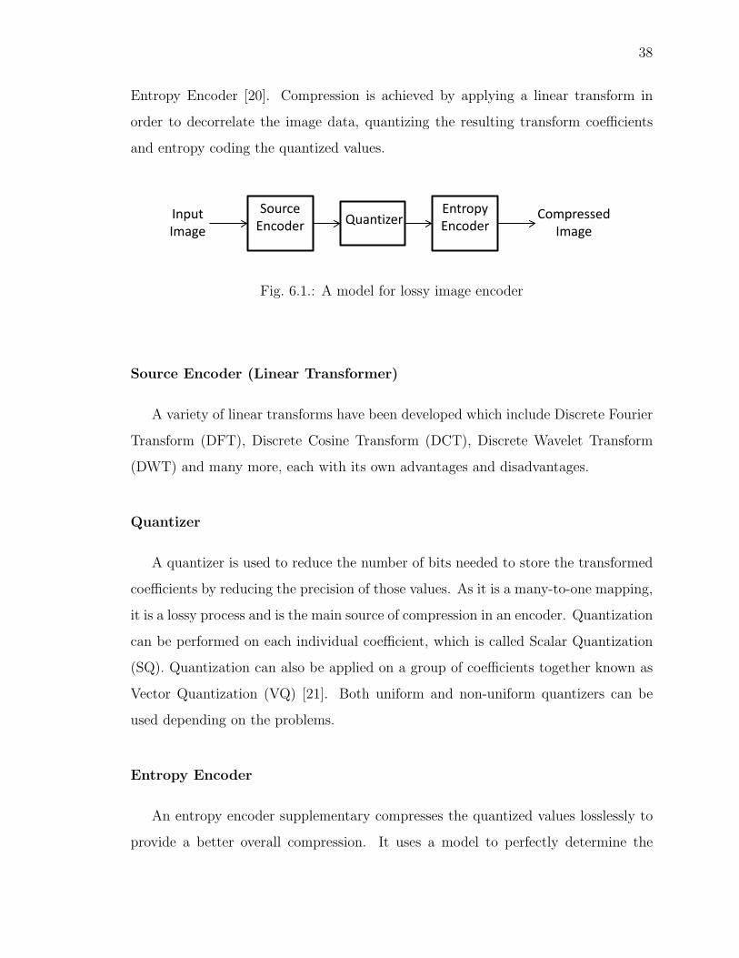
38

Entropy Encoder [20]. Compression is achieved by applying a linear transform in

order to decorrelate the image data, quantizing the resulting transform coefficients

and entropy coding the quantized values.

SourceEncoder Quantizer

EntropyEncoder

Input Image

CompressedImage

Fig. 6.1.: A model for lossy image encoder

Source Encoder (Linear Transformer)

A variety of linear transforms have been developed which include Discrete Fourier

Transform (DFT), Discrete Cosine Transform (DCT), Discrete Wavelet Transform

(DWT) and many more, each with its own advantages and disadvantages.

Quantizer

A quantizer is used to reduce the number of bits needed to store the transformed

coefficients by reducing the precision of those values. As it is a many-to-one mapping,

it is a lossy process and is the main source of compression in an encoder. Quantization

can be performed on each individual coefficient, which is called Scalar Quantization

(SQ). Quantization can also be applied on a group of coefficients together known as

Vector Quantization (VQ) [21]. Both uniform and non-uniform quantizers can be

used depending on the problems.

Entropy Encoder

An entropy encoder supplementary compresses the quantized values losslessly to

provide a better overall compression. It uses a model to perfectly determine the

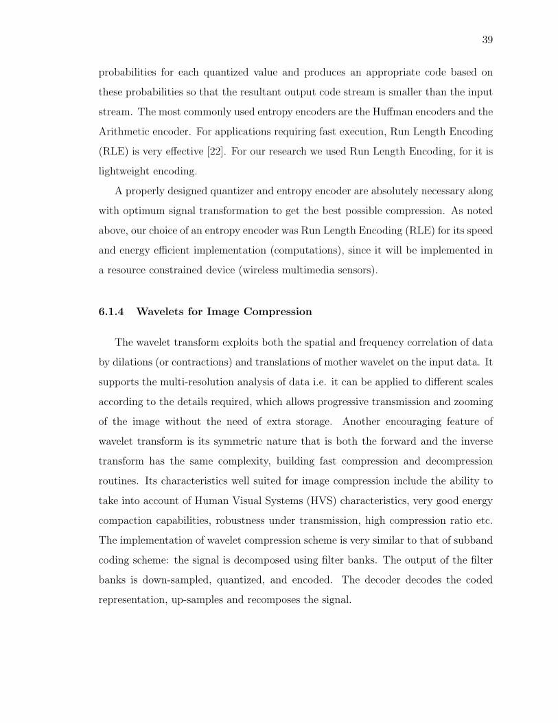
39

probabilities for each quantized value and produces an appropriate code based on

these probabilities so that the resultant output code stream is smaller than the input

stream. The most commonly used entropy encoders are the Huffman encoders and the

Arithmetic encoder. For applications requiring fast execution, Run Length Encoding

(RLE) is very effective [22]. For our research we used Run Length Encoding, for it is

lightweight encoding.

A properly designed quantizer and entropy encoder are absolutely necessary along

with optimum signal transformation to get the best possible compression. As noted

above, our choice of an entropy encoder was Run Length Encoding (RLE) for its speed

and energy efficient implementation (computations), since it will be implemented in

a resource constrained device (wireless multimedia sensors).

6.1.4 Wavelets for Image Compression

The wavelet transform exploits both the spatial and frequency correlation of data

by dilations (or contractions) and translations of mother wavelet on the input data. It

supports the multi-resolution analysis of data i.e. it can be applied to different scales

according to the details required, which allows progressive transmission and zooming

of the image without the need of extra storage. Another encouraging feature of

wavelet transform is its symmetric nature that is both the forward and the inverse

transform has the same complexity, building fast compression and decompression

routines. Its characteristics well suited for image compression include the ability to

take into account of Human Visual Systems (HVS) characteristics, very good energy

compaction capabilities, robustness under transmission, high compression ratio etc.

The implementation of wavelet compression scheme is very similar to that of subband

coding scheme: the signal is decomposed using filter banks. The output of the filter

banks is down-sampled, quantized, and encoded. The decoder decodes the coded

representation, up-samples and recomposes the signal.

40

Wavelet transform divides the information of an image into approximation and

detail subsignals. The approximation subsignal shows the general trend of pixel values

and other three detail subsignals show the vertical, horizontal and diagonal details or

changes in the images. If these details are very small, then they can be set to zero

(i.e. below some threshold) without significantly changing the image. The greater the

number of zeros the greater the compression ratio. If the energy retained (amount of

information retained by an image after compression and decompression) is 100% then

the compression is lossless as the image can be reconstructed exactly. This occurs

when the threshold value is set to zero, meaning that the details have not been

changed. If any value is changed then energy will be lost and thus lossy compression

occurs. As more zeros are obtained, more energy is lost. Therefore, a balance between

the two needs to be found out.

Fig. 6.2.: Wavelet decomposition of Lena (512× 512, L = 3)

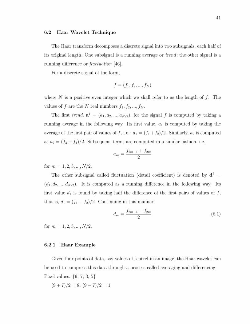
41

6.2 Haar Wavelet Technique

The Haar transform decomposes a discrete signal into two subsignals, each half of

its original length. One subsignal is a running average or trend ; the other signal is a

running difference or fluctuation [46].

For a discrete signal of the form,

f = (f1, f2, ..., fN)

where N is a positive even integer which we shall refer to as the length of f . The

values of f are the N real numbers f1, f2, ..., fN .

The first trend, a1 = (a1, a2, ..., aN/2), for the signal f is computed by taking a

running average in the following way. Its first value, a1 is computed by taking the

average of the first pair of values of f , i.e.: a1 = (f1 +f2)/2. Similarly, a2 is computed

as a2 = (f3 + f4)/2. Subsequent terms are computed in a similar fashion, i.e.

am =f2m−1 + f2m

2

for m = 1, 2, 3, ..., N/2.

The other subsignal called fluctuation (detail coefficient) is denoted by d1 =

(d1, d2, ..., dN/2). It is computed as a running difference in the following way. Its

first value d1 is found by taking half the difference of the first pairs of values of f ,

that is, d1 = (f1 − f2)/2. Continuing in this manner,

dm =f2m−1 − f2m

2(6.1)

for m = 1, 2, 3, ..., N/2.

6.2.1 Haar Example

Given four points of data, say values of a pixel in an image, the Haar wavelet can

be used to compress this data through a process called averaging and differencing.

Pixel values: {9, 7, 3, 5}

(9 + 7)/2 = 8, (9− 7)/2 = 1

42

(3 + 5)/2 = 4, (3− 5)/2 = −1

Coefficients: {8, 4, 1, ,1}

(8 + 4)/2 = 6, (8− 4)/2 = 2

Coefficients: {6 , 2, 1, 1}

There are two types of data here, sparse data and detailed data. The sparse data

is what we want to remove (in this example are the numbers {9,7,3,5,8,4,6}). The

other data are the details which make up the differences when doing our compression

(in this example they are {2,1,-1}).

But what good is compression that takes four values and compresses it to four

values? Simple, pixel values of images are similar to their neighbors. If not we would

be looking at random pixels and there would not be an object. When doing the

averaging and differencing with wavelets, the detail values are usually low numbers

and sometimes zero. These detail values (which compose all but one of the resulting

values) can be compressed much better than the original pixel values. In this example,

the number {6 2 1 1} are more easily compressible than {9 7 3 5}.

6.2.2 Filter Banks

As discussed above, there are two kinds of data, the sparse data and the detailed

data. Coefficients are extracted from the original set of number by using two kinds of

filters, high pass (details) and low pass (average). After the two filters are applied, the

filtered data from the high pass filter is stored as coefficients for later reconstruction

of the signal. The filtered data from the low pass filter is now treated as the original

data and the low and high pass filters are then applied to this data. This is repeated

until the filtered data from the low pass filter outputs only one number.

6.2.3 Image Thresholding

The main concept of the wavelet transform is: that regions of little variation in

the original image reveal themselves as small or zero elements in the wavelet trans-

43

formed version. The zeros are due to the occurrences of identical adjacent elements

in the original matrix. The coefficient matrix we get after the wavelet transform will

definitely be a sparse matrix (i.e.: with a high proportion of zero entries). For most

image matrices, their corresponding wavelet transformed versions are much sparser

than the original. Very sparse matrices are easier to store and transmit than ordinary

matrices of the same size. This is because the sparse matrices can be specified in the

data file by providing locations and values of their non-zero entries.

It can be seen that in the final transformed matrix (after the specified level of

decomposition, such as one level of decomposition (in our example above), we find

many entries are zero. From this transformed matrix, the original matrix can be

easily calculated just by the reverse operation of averaging and differencing i.e. the

original image can be reconstructed from the transformed image without the loss of

information (i.e. it yields a lossless compression). However, we need to achieve a

higher degree of compression, so we have to consider lossy compression that will give

us high compression ratio with reasonable (application specific) distortion amount.

In this case, a nonnegative threshold value say ε is set. Then any detail coefficient

in the transformed data whose magnitude is less than or equal to ε is set to zero.

It will increase the number of zeros in the transformed matrix and thus the level of

compression will be increased. So, ε = 0 would be used for a lossless compression. If a

lossy compression is used, an approximation of the original image can be constructed

with some reasonable loss of image fidelity (depending on the value of ε). The setting

of the threshold value is very important as there is a trade-off between the value of ε

and the quality of the compressed image. The different thresholding methods we have

used are: hard thresholding and soft thresholding. Note: for our experimental set up,

we used hard thresholding and the thresholding is not applied on the approximate

coefficient. These thresholding methods are defined as follows:

Hard Thresholding:

T (ε, x) =

0, if |x| < ε

x, otherwise

(6.2)

44

Soft Thresholding:

T (ε, x) =

0, if |x| < ε

sgn(x)(|x| − ε), otherwise

(6.3)

Note: For our experiment we used only hard thresholding for faster and energy

efficient execution, and the threshold is applied only on the detail coefficients (H, V

and D sub coefficients in the coefficient matrix). Also result of global thresholding

where a single threshold value (such as 20 in our experiment above) is used for all

levels (H,V and D),1 and level dependent thresholding where level and orientation

dependent thresholding is used. For example, a threshold value of 17 is used for H,

and 22 for D.

6.2.4 Procedures and Experimental Results

Multi-resolution, is concerned with the representation and analysis of images at

more than one resolution. For a Multi-Resolution Analysis (MRA), a scaling function

is used to create a series of functions called wavelets of an image, each differing by

a factor of 2 from its nearest neighboring approximations. The resulting filtered

output are approximation(A), vertical(V), horizontal(H) and diagonal(D) details of

the image. In this experiment we will be using Haar basis functions described in the

previous section. The Haar transform itself is both separable and symmetric and can

be expressed in matrix form [24]:

T = HFH (6.4)

where F is an N × N image, H is an N × N transformation matrix and T is the

resulting N × N transform. For the Haar transform, the transformation matrix H

contains the Haar basis functions, hk(z) for k = 0, 1, 2, ..., N − 1. The 2-dimensional

DWT of function f(x, y) of size M ×N is given by [24]:

1Here approximation(A), vertical(V), horizontal(H) and diagonal(D) details of the image.

45

WA(m,n) =

1√MN

M−1∑x=0

N−1∑y=0

f(x,y)hA(x,y) (6.5)

where WA(m,n) is the approximation image and hA(x,y) is the approximation coefficient.

W i(m,n) =

1√MN

M−1∑x=0

N−1∑y=0

f(x,y)hi(x,y) (6.6)

where i = {H,V,D} and hi(x,y) are the horizontal, vertical and diagonal coefficients.

6.2.5 Energy Efficient Local Processing Using DWT

Unlike a wired system where unlimited processing can be performed with no power

constraint, a wireless sensor (which is energy constrained) energy efficient signal pro-

cessing is needed to maximize the lifetime of the network. In a wireless sensor net-

work, communication is awkward and has a significant amount of power consumption.

When the distance between the sensors and between the sensors and the base station

increases, the energy spent in reliably transmitting data becomes costly. As discussed

in literature [28, 35, 36] that communication is the most power consuming operation

in wireless sensors, and the problem will be more exaggerated when the data is image

or video data (very large in size).

In our work here, we are providing an energy efficient technique that will trade

computation for communication as communication consumes more energy than com-

putation [28]. We are using multi-resolution image processing technique (DWT ,

with Haar filter), and transmitting the approximate coefficient and re-transmit more

refinement bits if the quality of the reconstructed image is below required by the

application.

Steps/Algorithms

Step 1 : Image acquisition by the sensor; upon external trigger by motion sensor, the

sensor starts acquiring image data I(m,n). Where Icurr(m,n) is the current image

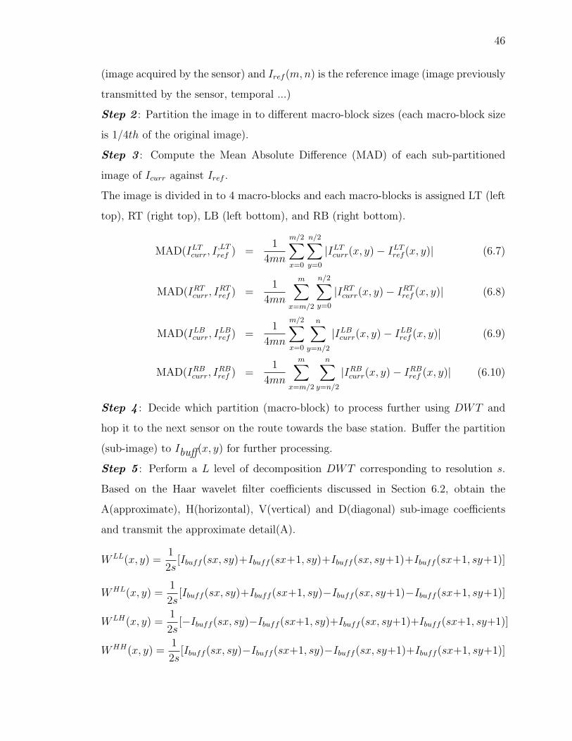
46

(image acquired by the sensor) and Iref (m,n) is the reference image (image previously

transmitted by the sensor, temporal ...)

Step 2 : Partition the image in to different macro-block sizes (each macro-block size

is 1/4th of the original image).

Step 3 : Compute the Mean Absolute Difference (MAD) of each sub-partitioned

image of Icurr against Iref .

The image is divided in to 4 macro-blocks and each macro-blocks is assigned LT (left

top), RT (right top), LB (left bottom), and RB (right bottom).

MAD(ILTcurr, I,LTref ) =

1

4mn

m/2∑x=0

n/2∑y=0

|ILTcurr(x, y)− ILTref (x, y)| (6.7)

MAD(IRTcurr, IRTref ) =

1

4mn

m∑x=m/2

n/2∑y=0

|IRTcurr(x, y)− IRTref (x, y)| (6.8)

MAD(ILBcurr, ILBref ) =

1

4mn

m/2∑x=0

n∑y=n/2

|ILBcurr(x, y)− ILBref (x, y)| (6.9)

MAD(IRBcurr, IRBref ) =

1

4mn

m∑x=m/2

n∑y=n/2

|IRBcurr(x, y)− IRBref (x, y)| (6.10)

Step 4 : Decide which partition (macro-block) to process further using DWT and

hop it to the next sensor on the route towards the base station. Buffer the partition

(sub-image) to Ibuff(x, y) for further processing.

Step 5 : Perform a L level of decomposition DWT corresponding to resolution s.

Based on the Haar wavelet filter coefficients discussed in Section 6.2, obtain the

A(approximate), H(horizontal), V(vertical) and D(diagonal) sub-image coefficients

and transmit the approximate detail(A).

WLL(x, y) =1

2s[Ibuff (sx, sy)+Ibuff (sx+1, sy)+Ibuff (sx, sy+1)+Ibuff (sx+1, sy+1)]

WHL(x, y) =1

2s[Ibuff (sx, sy)+Ibuff (sx+1, sy)−Ibuff (sx, sy+1)−Ibuff (sx+1, sy+1)]

WLH(x, y) =1

2s[−Ibuff (sx, sy)−Ibuff (sx+1, sy)+Ibuff (sx, sy+1)+Ibuff (sx+1, sy+1)]

WHH(x, y) =1

2s[Ibuff (sx, sy)−Ibuff (sx+1, sy)−Ibuff (sx, sy+1)+Ibuff (sx+1, sy+1)]

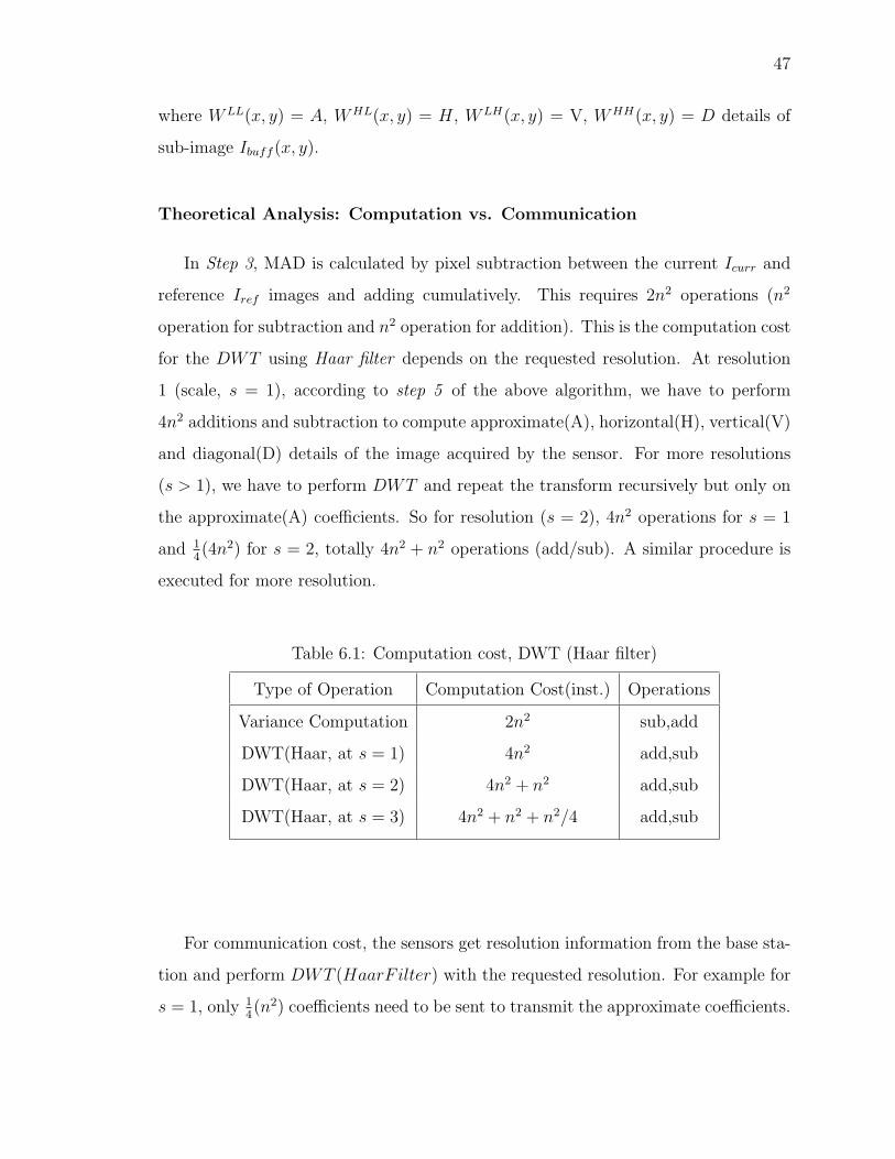
47

where WLL(x, y) = A, WHL(x, y) = H, WLH(x, y) = V, WHH(x, y) = D details of

sub-image Ibuff (x, y).

Theoretical Analysis: Computation vs. Communication

In Step 3, MAD is calculated by pixel subtraction between the current Icurr and

reference Iref images and adding cumulatively. This requires 2n2 operations (n2

operation for subtraction and n2 operation for addition). This is the computation cost

for the DWT using Haar filter depends on the requested resolution. At resolution

1 (scale, s = 1), according to step 5 of the above algorithm, we have to perform

4n2 additions and subtraction to compute approximate(A), horizontal(H), vertical(V)

and diagonal(D) details of the image acquired by the sensor. For more resolutions

(s > 1), we have to perform DWT and repeat the transform recursively but only on

the approximate(A) coefficients. So for resolution (s = 2), 4n2 operations for s = 1

and 14(4n2) for s = 2, totally 4n2 + n2 operations (add/sub). A similar procedure is

executed for more resolution.

Table 6.1: Computation cost, DWT (Haar filter)

Type of Operation Computation Cost(inst.) Operations

Variance Computation 2n2 sub,add

DWT(Haar, at s = 1) 4n2 add,sub

DWT(Haar, at s = 2) 4n2 + n2 add,sub

DWT(Haar, at s = 3) 4n2 + n2 + n2/4 add,sub

For communication cost, the sensors get resolution information from the base sta-

tion and perform DWT (HaarFilter) with the requested resolution. For example for

s = 1, only 14(n2) coefficients need to be sent to transmit the approximate coefficients.

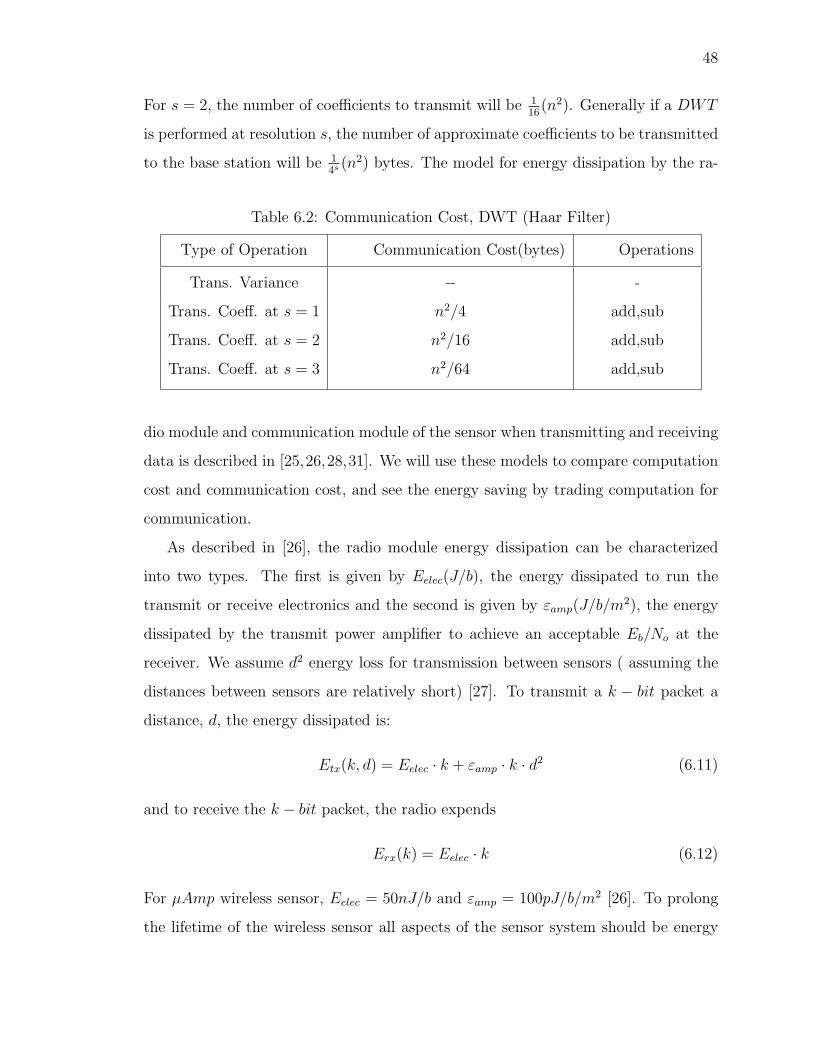
48

For s = 2, the number of coefficients to transmit will be 116

(n2). Generally if a DWT

is performed at resolution s, the number of approximate coefficients to be transmitted

to the base station will be 14s (n2) bytes. The model for energy dissipation by the ra-

Table 6.2: Communication Cost, DWT (Haar Filter)

Type of Operation Communication Cost(bytes) Operations

Trans. Variance − -

Trans. Coeff. at s = 1 n2/4 add,sub



dio module and communication module of the sensor when transmitting and receiving

data is described in [25,26,28,31]. We will use these models to compare computation

cost and communication cost, and see the energy saving by trading computation for

communication.

As described in [26], the radio module energy dissipation can be characterized

into two types. The first is given by Eelec(J/b), the energy dissipated to run the

transmit or receive electronics and the second is given by εamp(J/b/m2), the energy

dissipated by the transmit power amplifier to achieve an acceptable Eb/No at the

receiver. We assume d2 energy loss for transmission between sensors ( assuming the

distances between sensors are relatively short) [27]. To transmit a k − bit packet a

distance, d, the energy dissipated is:

Etx(k, d) = Eelec · k + εamp · k · d2 (6.11)

and to receive the k − bit packet, the radio expends

Erx(k) = Eelec · k (6.12)

For µAmp wireless sensor, Eelec = 50nJ/b and εamp = 100pJ/b/m2 [26]. To prolong

the lifetime of the wireless sensor all aspects of the sensor system should be energy

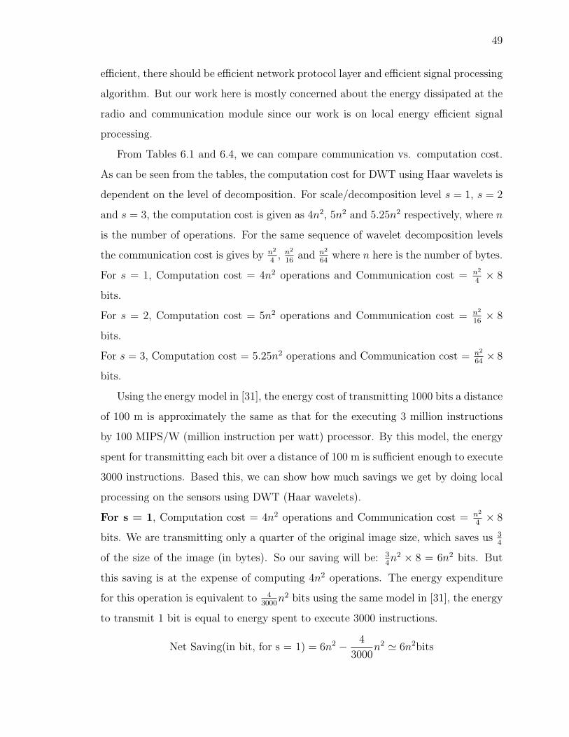
49

efficient, there should be efficient network protocol layer and efficient signal processing

algorithm. But our work here is mostly concerned about the energy dissipated at the

radio and communication module since our work is on local energy efficient signal

processing.

From Tables 6.1 and 6.4, we can compare communication vs. computation cost.

As can be seen from the tables, the computation cost for DWT using Haar wavelets is

dependent on the level of decomposition. For scale/decomposition level s = 1, s = 2

and s = 3, the computation cost is given as 4n2, 5n2 and 5.25n2 respectively, where n

is the number of operations. For the same sequence of wavelet decomposition levels

the communication cost is gives by n2

4, n2

16and n2

64where n here is the number of bytes.

For s = 1, Computation cost = 4n2 operations and Communication cost = n2

4× 8

bits.


16× 8

bits.

For s = 3, Computation cost = 5.25n2 operations and Communication cost = n2

64× 8

bits.

Using the energy model in [31], the energy cost of transmitting 1000 bits a distance

of 100 m is approximately the same as that for the executing 3 million instructions

by 100 MIPS/W (million instruction per watt) processor. By this model, the energy

spent for transmitting each bit over a distance of 100 m is sufficient enough to execute

3000 instructions. Based this, we can show how much savings we get by doing local

processing on the sensors using DWT (Haar wavelets).


4× 8

bits. We are transmitting only a quarter of the original image size, which saves us 34

of the size of the image (in bytes). So our saving will be: 34n2 × 8 = 6n2 bits. But

this saving is at the expense of computing 4n2 operations. The energy expenditure

for this operation is equivalent to 43000

n2 bits using the same model in [31], the energy

to transmit 1 bit is equal to energy spent to execute 3000 instructions.

Net Saving(in bit, for s = 1) = 6n2 − 4

3000n2 ' 6n2bits

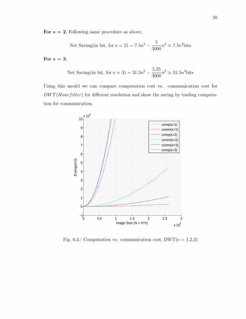
50

For s = 2, Following same procedure as above,

Net Saving(in bit, for s = 2) = 7.5n2 − 5

3000n2 ' 7.5n2bits

For s = 3,

Net Saving(in bit, for s = 3) = 31.5n2 − 5.25

3000n2 ' 31.5n2bits

Using this model we can compare computation cost vs. communication cost for

DWT (Haarfilter) for different resolution and show the saving by trading computa-

tion for communication.

0 0.5 1 1.5 2 2.5 3

x 105

−1

0

1

2

3

4

5

6

7

8

9

10x 10

5

Image Size (N = m*n)

En

erg

y(n

J)

comp(s=1)comm(s=1)comp(s=2)comm(s=2)comm(s=3)comp(s=3)

Fig. 6.3.: Computation vs. communication cost, DWT(s = 1,2,3)

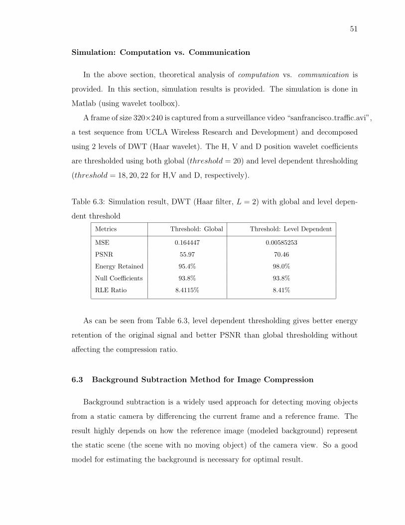
51

Simulation: Computation vs. Communication

In the above section, theoretical analysis of computation vs. communication is

provided. In this section, simulation results is provided. The simulation is done in

Matlab (using wavelet toolbox).

A frame of size 320×240 is captured from a surveillance video “sanfrancisco traffic.avi”,

a test sequence from UCLA Wireless Research and Development) and decomposed

using 2 levels of DWT (Haar wavelet). The H, V and D position wavelet coefficients

are thresholded using both global (threshold = 20) and level dependent thresholding

(threshold = 18, 20, 22 for H,V and D, respectively).

Table 6.3: Simulation result, DWT (Haar filter, L = 2) with global and level depen-

dent threshold

Metrics Threshold: Global Threshold: Level Dependent

MSE 0.164447 0.00585253

PSNR 55.97 70.46

Energy Retained 95.4% 98.0%

Null Coefficients 93.8% 93.8%

RLE Ratio 8.4115% 8.41%

As can be seen from Table 6.3, level dependent thresholding gives better energy

retention of the original signal and better PSNR than global thresholding without

affecting the compression ratio.

6.3 Background Subtraction Method for Image Compression

Background subtraction is a widely used approach for detecting moving objects

from a static camera by differencing the current frame and a reference frame. The

result highly depends on how the reference image (modeled background) represent

the static scene (the scene with no moving object) of the camera view. So a good

model for estimating the background is necessary for optimal result.

52

6.3.1 Background Model - Estimating Good Background

Several methods of performing background subtraction have been proposed in

literature [67]. All these methods try to estimate the background model from the

temporal sequence of the frames, each method with its benefits and limitations. In the

next section, we provide some of these common techniques based on speed, memory

requirement and accuracy.

6.3.2 The Most Common Approaches of Background Modeling

The approaches below range from simple approaches, aiming to maximize speed

and limiting the memory requirement to more sophisticated approaches aiming to

achieve the highest possible accuracy. Some of these are Running Gaussian Aver-

age, Temporal Median Filter, Gaussian Mixture Model, Kernel Density Estimation

(KDE), Sequential KD Approximation, etc.

As discussed in Section 2.2.2, three common approaches are:

• Running Gaussian Average

• Temporal Median Filter

• Gaussian Mixture Model

6.3.3 Foreground Processing

The background for our model is created by using the Gaussian running average

model, Equation (2.1) described in Section 2.2.2. The value for α in Equation (2.1)

is set to 0.075 and a background is created using a static scene.

For each current frame, a foreground object (Ifg) is extracted/created by sub-

tracting the background image (IB) from the current frame (IC) as follows.

53

Ifg = IC − IB (6.13)

IR = Ifg + IB (6.14)

If the frame is a 256 level grayscale, both the values of IB and IC ranges between

0 and 255 which requires 8 bits to encode each of the pixels. But the foreground

image Ifg have values 511 distinct values between −255 to 255, which needs 9 bits

to encode each value. We have proposed an algorithm to reduce the number of bits

used to encode each pixel during Run Length Encoding in the next subsection.

6.3.4 Improving the Run Length Encoder

As we have noted the range of values in Ifg are -255 to +255. After applying a

simple run-length encoding to the foreground, we transmit it as,

pixel run pixel run pixel run...

The goal of this encoding scheme is based on the assumption that the length of the

byte stream should be much less than the original image since there is much redundant

data (mostly zeros) in the foreground image.

Transmitting the Foreground Image, if the frame is a 256 level grayscale,

both the values of IB and IC ranges from 0 to 255 which requires only 8 bits to

encode each pixel. But the foreground image Ifg have 511 distinct values ranging

between −255 and 255, which requires 9 bits to encode.

Most commercial sensors like MCU(ATMEL 90LS8535) and TinyOS comes with

8 bit cpu and store data in 8 bit chunk. An actual implementation that takes (for

example) 8 bit input must store each 9 bit coefficient in a data type 16 bits wide,

thus consuming twice the memory bandwidth.

Our Solution for this Problem, thresholding by dividing each pixel in the

foreground image by an appropriate value. If we divide by two, we obtain Ifg/2,

54

which produces a range of values between −127 and 127 which is 255 distinct vales.

Now 8 bits is required to encode this values. The maximum run now is 255. In

this case each pixel value of the image is encoded as a pixel and run byte wise, e.g:

56, 56, 56, 56, 57, 125, 124, 124, 124 is encoded as 56, 4, 57, 1, 125, 1, 124, 3.

For example, if we divide the foreground by four, we obtain Ifg/4, which will make

the range of values [−63, 63], then adding the shift (64), we will have a range of values

[1, 127] which requires only 7 bits to encode. The eighth bit can be used as a flag bit

to represent if that value is a pixel value or a run count (e.g. eighth bit equals 1 for

pixel and zero for run count). Advantage of this scheme, in an 8 bit OS controller,

we need only 7 bits to encode each pixel value of the foreground. Thus, the high bit

can be used a flag to indicate if that value is a pixel or a run count. During decoding

of the image the reverse operation has to be done to recover the correct values of the

foreground pixel.

pixel pixel pixel run pixel run...

The maximum run now is 127. In this case the run will be counted bitwise, where

the high bit is used as a flag to indicate if that byte is a pixel value or a run count.

If we divide the fore ground by 8, we obtain Ifg/8, will make the range of values

between −32 and 32 which is 65 distinct vales and 6 bit is required to encode this

values. It can be encoded as a 7 bit value plus a bit to flag if it is a pixel value or a

run count. The maximum run now is 32.

Generally, if the divisor during quantization is greater than 4 and we view the

byte as a bitstream, we can encode pixel with less bits.

• D = 8, needs only 7 bits (6 bits for pixel value and 1 bit for flag), maxrun = 26



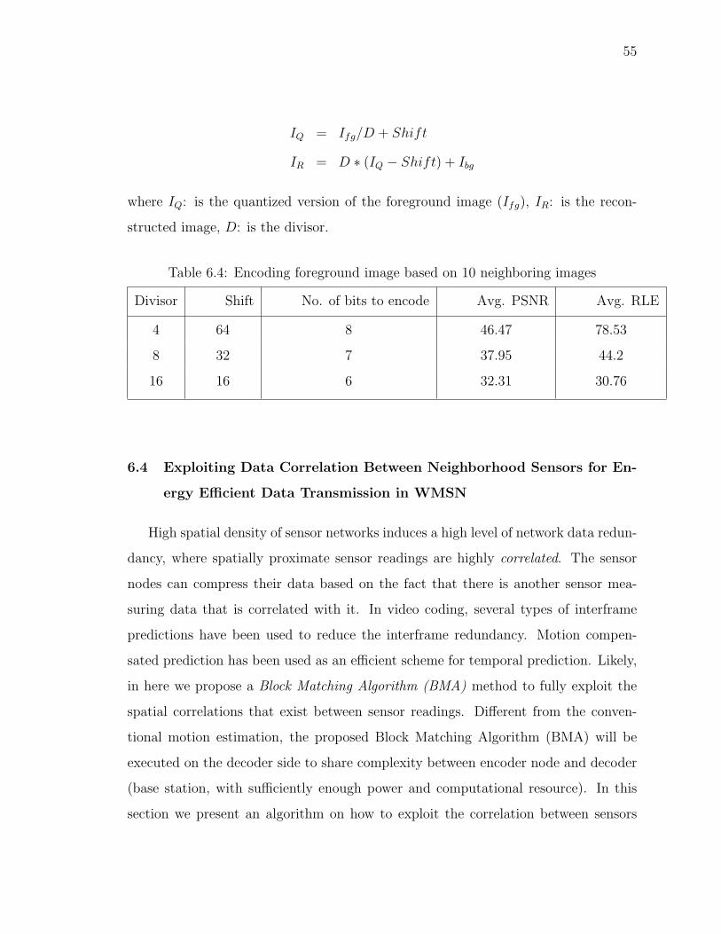
55

IQ = Ifg/D + Shift

IR = D ∗ (IQ − Shift) + Ibg

where IQ: is the quantized version of the foreground image (Ifg), IR: is the recon-

structed image, D: is the divisor.

Table 6.4: Encoding foreground image based on 10 neighboring images

Divisor Shift No. of bits to encode Avg. PSNR Avg. RLE

4 64 8 46.47 78.53

8 32 7 37.95 44.2

16 16 6 32.31 30.76

6.4 Exploiting Data Correlation Between Neighborhood Sensors for En-

ergy Efficient Data Transmission in WMSN

High spatial density of sensor networks induces a high level of network data redun-

dancy, where spatially proximate sensor readings are highly correlated. The sensor

nodes can compress their data based on the fact that there is another sensor mea-

suring data that is correlated with it. In video coding, several types of interframe

predictions have been used to reduce the interframe redundancy. Motion compen-

sated prediction has been used as an efficient scheme for temporal prediction. Likely,

in here we propose a Block Matching Algorithm (BMA) method to fully exploit the

spatial correlations that exist between sensor readings. Different from the conven-

tional motion estimation, the proposed Block Matching Algorithm (BMA) will be

executed on the decoder side to share complexity between encoder node and decoder

(base station, with sufficiently enough power and computational resource). In this

section we present an algorithm on how to exploit the correlation between sensors

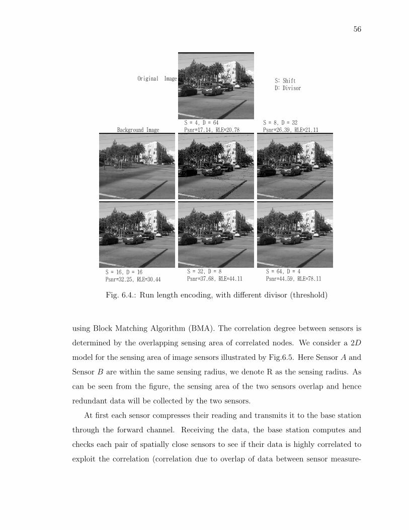
56

Background Image

S = 64, D = 4Psnr=44.59, RLE=78.11

S: ShiftD: Divisor

S = 32, D = 8Psnr=37.68, RLE=44.11

S = 16, D = 16Psnr=32.25, RLE=30.44

S = 8, D = 32Psnr=26.39, RLE=21.11

S = 4, D = 64Psnr=17.14, RLE=20.78

Original Image

Fig. 6.4.: Run length encoding, with different divisor (threshold)

using Block Matching Algorithm (BMA). The correlation degree between sensors is

determined by the overlapping sensing area of correlated nodes. We consider a 2D

model for the sensing area of image sensors illustrated by Fig.6.5. Here Sensor A and

Sensor B are within the same sensing radius, we denote R as the sensing radius. As

can be seen from the figure, the sensing area of the two sensors overlap and hence

redundant data will be collected by the two sensors.

At first each sensor compresses their reading and transmits it to the base station

through the forward channel. Receiving the data, the base station computes and

checks each pair of spatially close sensors to see if their data is highly correlated to

exploit the correlation (correlation due to overlap of data between sensor measure-

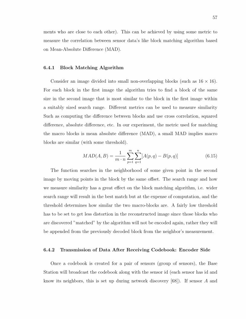
57

ments who are close to each other). This can be achieved by using some metric to

measure the correlation between sensor data’s like block matching algorithm based

on Mean-Absolute Difference (MAD).

6.4.1 Block Matching Algorithm

Consider an image divided into small non-overlapping blocks (such as 16 × 16).

For each block in the first image the algorithm tries to find a block of the same

size in the second image that is most similar to the block in the first image within

a suitably sized search range. Different metrics can be used to measure similarity

Such as computing the difference between blocks and use cross correlation, squared

difference, absolute difference, etc. In our experiment, the metric used for matching

the macro blocks is mean absolute difference (MAD), a small MAD implies macro

blocks are similar (with some threshold).

MAD(A,B) =1

m · n

m∑p=1

n∑q=1

[A(p, q)−B(p, q)] (6.15)

The function searches in the neighborhood of some given point in the second

image by moving points in the block by the same offset. The search range and how

we measure similarity has a great effect on the block matching algorithm, i.e. wider

search range will result in the best match but at the expense of computation, and the

threshold determines how similar the two macro-blocks are. A fairly low threshold

has to be set to get less distortion in the reconstructed image since those blocks who

are discovered ”matched” by the algorithm will not be encoded again, rather they will

be appended from the previously decoded block from the neighbor’s measurement.

6.4.2 Transmission of Data After Receiving Codebook: Encoder Side

Once a codebook is created for a pair of sensors (group of sensors), the Base

Station will broadcast the codebook along with the sensor id (each sensor has id and

know its neighbors, this is set up during network discovery [68]). If sensor A and

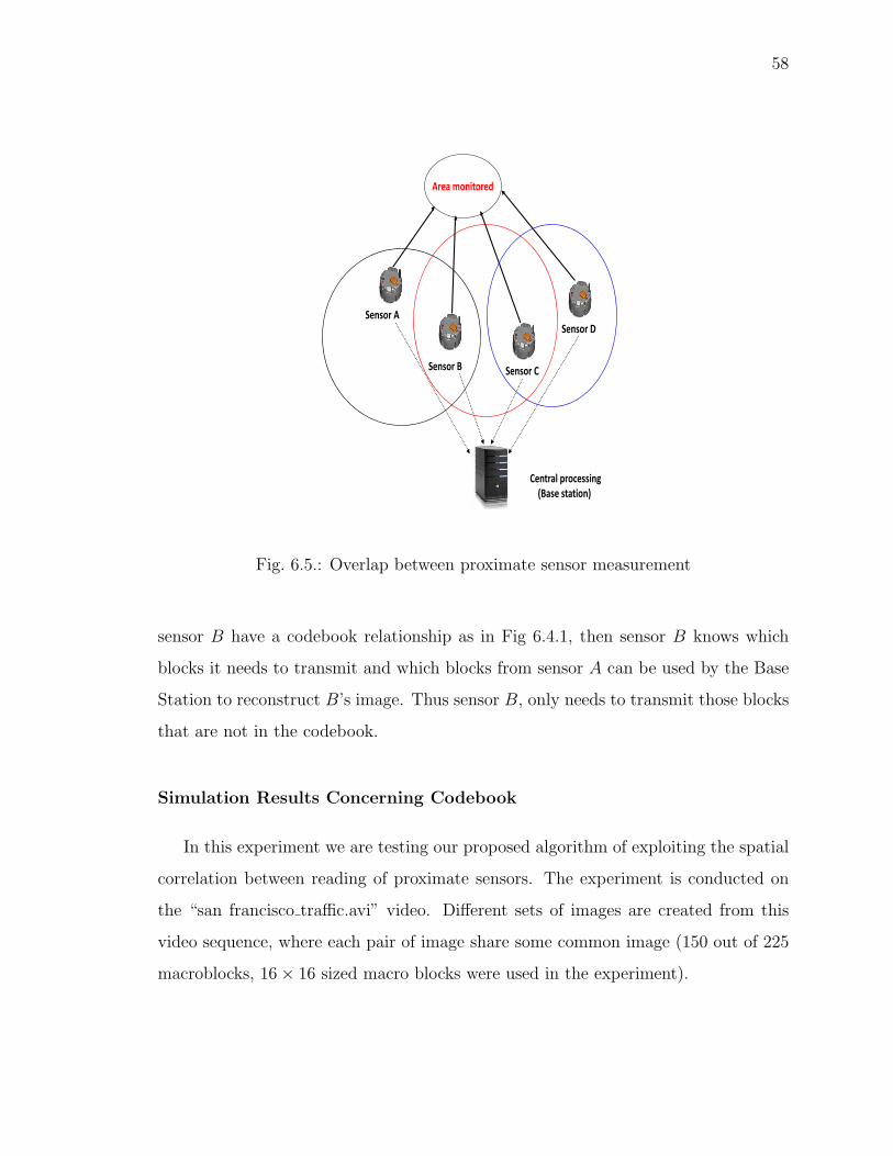
58

Sensor ASensor D

Sensor CSensor B

Area monitored

Central processing (Base station)

Fig. 6.5.: Overlap between proximate sensor measurement

sensor B have a codebook relationship as in Fig 6.4.1, then sensor B knows which

blocks it needs to transmit and which blocks from sensor A can be used by the Base

Station to reconstruct B’s image. Thus sensor B, only needs to transmit those blocks

that are not in the codebook.

Simulation Results Concerning Codebook

In this experiment we are testing our proposed algorithm of exploiting the spatial

correlation between reading of proximate sensors. The experiment is conducted on

the “san francisco traffic.avi” video. Different sets of images are created from this

video sequence, where each pair of image share some common image (150 out of 225

macroblocks, 16× 16 sized macro blocks were used in the experiment).

59

Experiment:

Each pair of image (frame) is partitioned into blocks of 16 × 16, and a Block

matching algorithm will be run on each pair of images to exploit the overlap area and

those blocks within the pair are found to be matched if their MAD are within the

given threshold, these blocks will then be flagged.

There are different factors affecting the efficiency of the codebook method. Some

of these are, the choice of threshold, the choice of the number of frames used to build

the codebook, etc.

Choosing an appropriate threshold is vital for getting an efficient codebook with

minimal false positives. The higher the threshold, the more the probability that a false

match will occur. The number of frames used to create the codebook will also affect

how good the codebook will be. The more frames we used to create the codebook,

the less the number of matched blocks will be since we are using all or none approach

(i.e.: on a specific macro block all the frames used to compute the codebook has to

agree that it is a match, else it will not be added in the codebook). Table 6.5 shows

the creation of codebook using different threshold and different frames.

Analyzing the results in Table 6.5, as stated above the two images are created

so that they have overlap of 150 macroblocks out of the total 225 macro block in

each frame. With 0 thresholding and a single frame to create the codebook we have

retrieved all the overlapped macroblocks (look at first row of Table 6.5), but with same

threshold and 5 frames to create the codebook we have lost only a single macro block

due to a false positive (row 4 of Table 6.5), and same result for with 0 threshold and 10

frames to create the codebook, all with a very good PSNR value. With threshold = 3

and a single frame to create the codebook, we have 198 macroblocks matched, which

is higher than the total overlapped macroblocks between the two frames, this implies

there are many false matches and the quality of the reconstructed image is expected

to degrade (psnr = 19.02, row 2 of Table 6.5). With 5 frames to create the codebook,

the number of matched macroblocks drops dramatically from 198 to 3, this saving

60

(which has only 3 macro block) is insignificant and the psnr is expected to be very

high (psnr = INF (infinity)), and same result using 10 macroblocks to create the

codebook. With threshold = 9 and a single frame to create the codebook, we have

216 matched macroblocks, lot of false matches and hence degraded reconstructed

frame (psnr = 14.90). With 5 and 10 frames to create the codebook, only a single

macro block match is found and the reconstructed image is of almost same quality as

the original (psnr = INF ).

From Table 6.5 and the analysis in the above paragraph, it can be deduced that

the threshold and number of frames used to create the codebook has to be chosen

carefully to get a good saving by using the codebook method. In our experiment, the

results in row 4 and 7 in Table 6.5 have optimal values.

ref image threshold is

(a) Original Image

threshold is0 #frames to build codeBK1 identified blocks150 out of225

(b) Thresh = 0, Frame = 1, Match = 150

Fig. 6.6.: Reference image vs. frame with threshold = 0

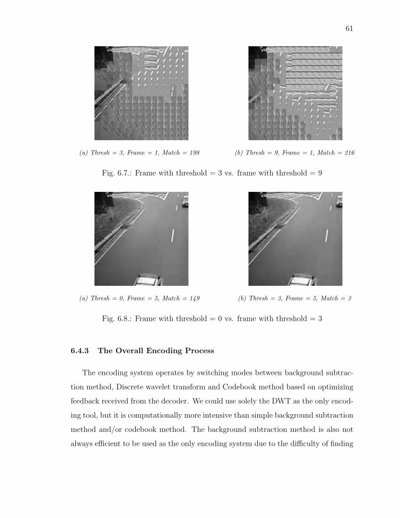
61


(a) Thresh = 3, Frame = 1, Match = 198



Fig. 6.7.: Frame with threshold = 3 vs. frame with threshold = 9






6.4.3 The Overall Encoding Process

The encoding system operates by switching modes between background subtrac-

tion method, Discrete wavelet transform and Codebook method based on optimizing

feedback received from the decoder. We could use solely the DWT as the only encod-

ing tool, but it is computationally more intensive than simple background subtraction

method and/or codebook method. The background subtraction method is also not

always efficient to be used as the only encoding system due to the difficulty of finding

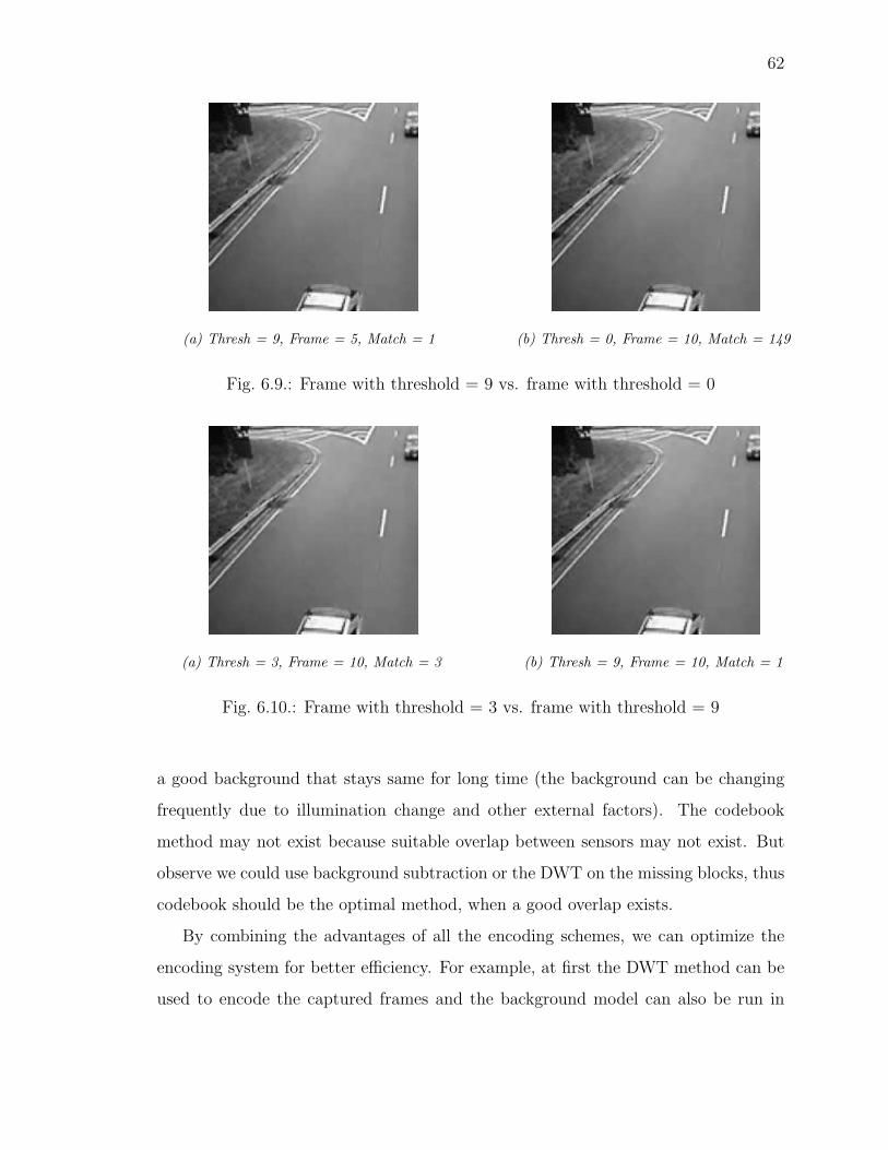
62











a good background that stays same for long time (the background can be changing

frequently due to illumination change and other external factors). The codebook

method may not exist because suitable overlap between sensors may not exist. But

observe we could use background subtraction or the DWT on the missing blocks, thus

codebook should be the optimal method, when a good overlap exists.

By combining the advantages of all the encoding schemes, we can optimize the

encoding system for better efficiency. For example, at first the DWT method can be

used to encode the captured frames and the background model can also be run in

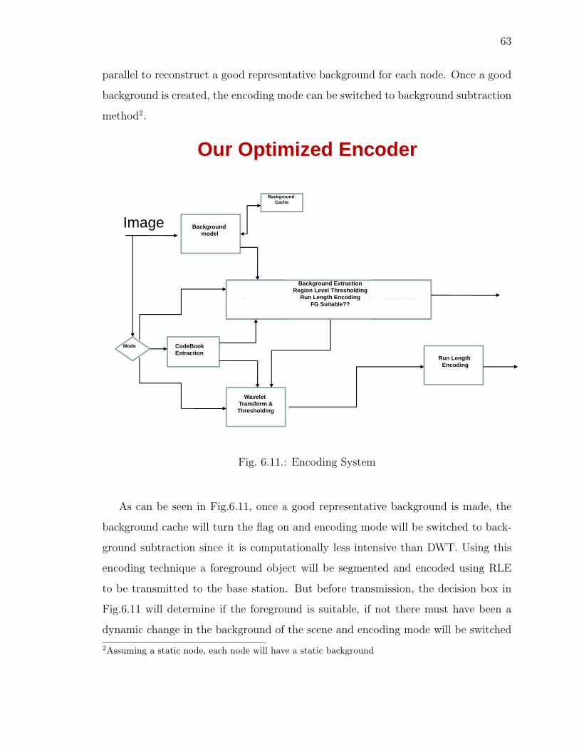
63

parallel to reconstruct a good representative background for each node. Once a good

background is created, the encoding mode can be switched to background subtraction

method2.

Our Optimized Encoder

Background Cache

Ou Opt ed code

Background model

Cache

Image

BackgroundE t ti

Region LevelThresholding

FGSuitable??Back

Background ExtractionRegion Level Thresholding

Run Length EncodingExtraction

CodeBook

Thresholding

Mode

acRun Length EncodingFG Suitable??

CodeBookExtraction

Run Length Encoding

Mode

Wavelet Transform &Thresholding

Fig. 6.11.: Encoding System

As can be seen in Fig.6.11, once a good representative background is made, the

background cache will turn the flag on and encoding mode will be switched to back-

ground subtraction since it is computationally less intensive than DWT. Using this

encoding technique a foreground object will be segmented and encoded using RLE

to be transmitted to the base station. But before transmission, the decision box in

Fig.6.11 will determine if the foreground is suitable, if not there must have been a

dynamic change in the background of the scene and encoding mode will be switched

2Assuming a static node, each node will have a static background

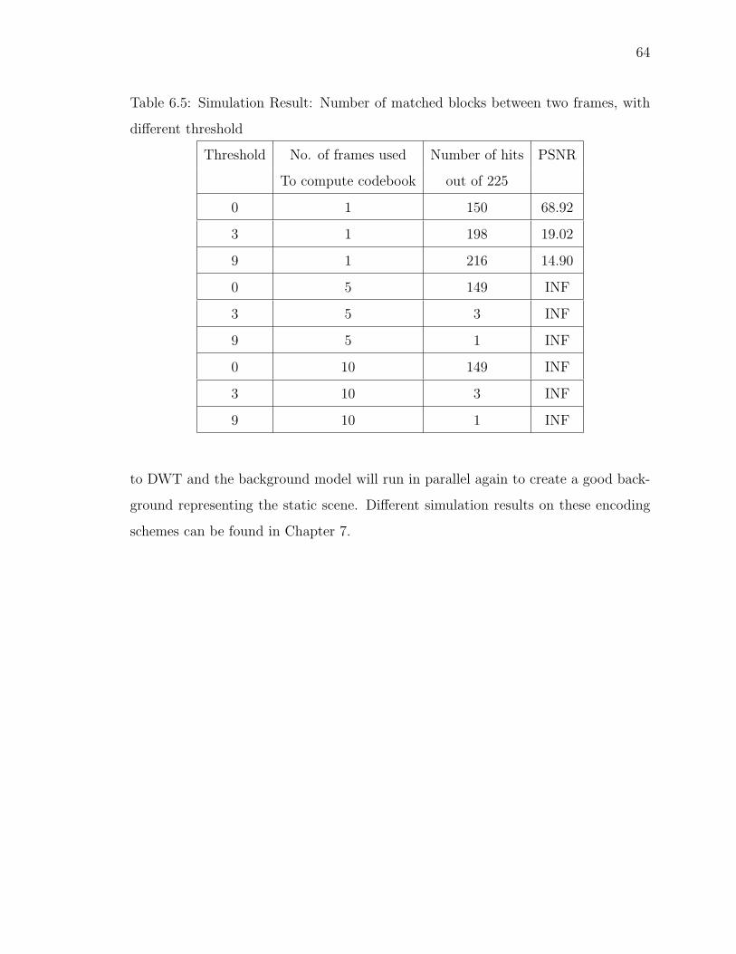
64

Table 6.5: Simulation Result: Number of matched blocks between two frames, with

different threshold

Threshold No. of frames used Number of hits PSNR

To compute codebook out of 225

0 1 150 68.92

3 1 198 19.02

9 1 216 14.90

0 5 149 INF

3 5 3 INF

9 5 1 INF

0 10 149 INF

3 10 3 INF

9 10 1 INF

to DWT and the background model will run in parallel again to create a good back-

ground representing the static scene. Different simulation results on these encoding

schemes can be found in Chapter 7.

65

7. IMAGE QUALITY ASSESSMENT BY BASE STATION

7.1 Introduction

As described in Chapter 6, upon receiving the compressed signal from the sen-

sors, the base station need to decode and reconstruct the image. Once the image

is reconstructed the quality of the reconstructed signal has to be evaluated and the

information has to be transmitted back to the encoding system through the backward

channel. First for requesting re-transmission of the previous signal if the quality of

the reconstructed signal is below the quality required by the application, and second

to optimize algorithms and parameter settings of the encoding system.

Many efficient techniques have been developed to evaluate the quality of the re-

constructed image for both lossless or lossy type of compression. The evaluation

technique for lossless type of compression is straight forward since there will not be

loss of information during the encoding process. The algorithm will be evaluated

based on compression ratio, how fast the encoding process will be executed to be

applied for real time applications and so on. Such an evaluation is outside the scope

of the base station’s concerns. Furthermore the compression techniques that we are

implementing are certainly lossy. For lossy compression techniques the major prob-

lem in evaluating them, is the difficulty in type and amount of degradation in the

reconstructed image.

Since the main objective of our work is on energy efficient image and video pro-

cessing and transmission in wireless sensor networks, we won’t be able to send more

information about the original signal besides its compressed version. The only infor-

mation available in the base station side is information from the reconstructed image;

i.e. the decoder won’t be able to use the common image quality assessment tools to

66

give feedback to the encoding system or to optimize the parameters in the encoding

algorithm.

7.2 Image Quality Assessment Tools

Objective image and video quality metrics can be classified in to three broad

categories based on the availability of the original image and video signal [73]:

Full-Reference (FR) QA methods, in which the QA algorithm has access to a

perfect version of the image or video against which it can compare a distorted version.

The perfect version generally comes from a high-quality acquisition device, before it

is distorted by compression artifacts and transmission errors. However, the reference

image or video generally requires much more resources than the distorted version,

and hence FR QA is generally only used as a tool for designing image and video

processing algorithms for in-lab testing, and cannot be deployed as an application.

Currently the most widely used objective image and video fidelity (distortion)

metrics are Mean Square Error (MSE) and Peak Signal to Noise Ration (PSNR).

MSE =1

N

N∑i=1

(xi − yi)2 (7.1)

PSNR = 10 log10

L2

MSE(7.2)

where N is the number of pixels in the image or video signal, and xi and yi are the

ith pixel in the original and distorted signals respectively. L is the dynamic range of

the pixel (for an 8 bits per pixel monotonic signal L is equal to 255).

An objective image and video quality measure metric that is commonly used is the

Structural Similarity Index (SSIM) [18]. It is a full reference metric, i.e. it measures

image quality based on an initial uncompressed or distortion-free image as reference.

SSIM is designed to improve on traditional methods like peak signal-to-noise ratio

(PSNR) and mean squared error (MSE), which have proved to be inconsistent with

human eye perception.

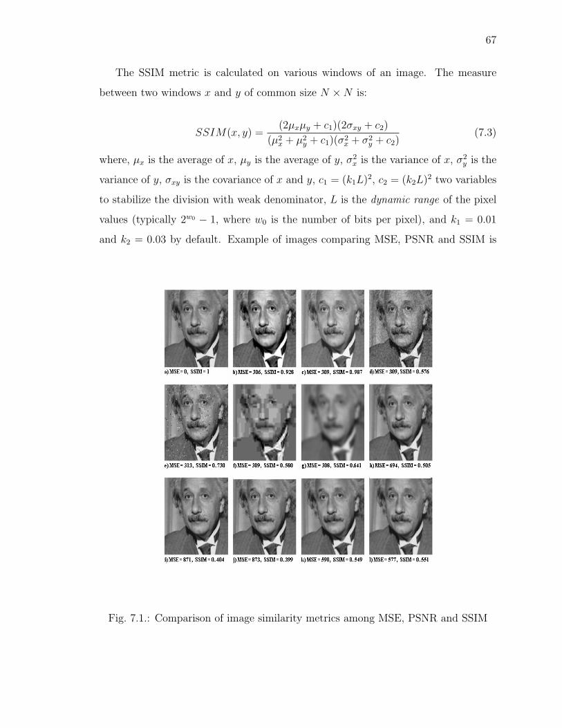
67

The SSIM metric is calculated on various windows of an image. The measure

between two windows x and y of common size N ×N is:

SSIM(x, y) =(2µxµy + c1)(2σxy + c2)

(µ2x + µ2

y + c1)(σ2x + σ2

y + c2)(7.3)

where, µx is the average of x, µy is the average of y, σ2x is the variance of x, σ2

y is the

variance of y, σxy is the covariance of x and y, c1 = (k1L)2, c2 = (k2L)2 two variables

to stabilize the division with weak denominator, L is the dynamic range of the pixel

values (typically 2w0 − 1, where w0 is the number of bits per pixel), and k1 = 0.01

and k2 = 0.03 by default. Example of images comparing MSE, PSNR and SSIM is

Fig. 7.1.: Comparison of image similarity metrics among MSE, PSNR and SSIM

68

given in Fig.7.1. The problem with this approach is that it requires the covariance

and so both the reference image and the reconstructed image is needed.

No-Reference (NR) QA methods, in which the QA algorithm has access only to the

distorted signal and must estimate the quality of the signal without any knowledge of

the perfect version. Since NR methods do not require any reference information, they

can be used in any application where a quality measurement is required. However,

the price paid for this flexibility is in terms of the ability of the algorithm to make

accurate quality predictions, or a limited scope of the NR QA algorithm (such as NR

QA for JPEG images only etc.).

Although this type of image and video quality assessment tool is very efficient for

our research to optimize the encoding system with out sending side information to

the station, there is no general metric available to accurately measure the similarity

between two images with out having the original (or some side information about

the original) image or video at the base station (decoder) side. Several NR quality

assessment applications have been addressed in [73] and [19].

Reduced-Reference (RR) QA methods, in which partial information regarding the

“perfect version” is available. A side-channel (called an RR channel) exists through

which some information regarding the reference can be made available to the QA

algorithm. RR QA algorithms use this partial reference information to judge the

quality of the distorted signal.

Our work uses Reduced-Reference (RR) QA method, where some side information

besides the compressed version of the image is sent to the decoder (base station) using

the side channel.

7.3 Reduced-Reference (RR) QA Methods, Our Approach (Technique)

In our approach we considered three different metrics that the Base Station could

use to evaluate the quality of the reconstructed image at the base station. These are

Thumbnail PSNR, Mean test and Variance test.

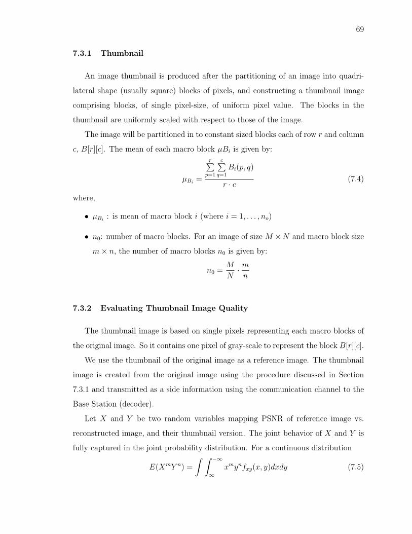
69

7.3.1 Thumbnail

An image thumbnail is produced after the partitioning of an image into quadri-

lateral shape (usually square) blocks of pixels, and constructing a thumbnail image

comprising blocks, of single pixel-size, of uniform pixel value. The blocks in the

thumbnail are uniformly scaled with respect to those of the image.

The image will be partitioned in to constant sized blocks each of row r and column

c, B[r][c]. The mean of each macro block µBi is given by:

µBi=

r∑p=1

c∑q=1

Bi(p, q)

r · c(7.4)

where,

• µBi: is mean of macro block i (where i = 1, . . . , no)

• n0: number of macro blocks. For an image of size M ×N and macro block size

m× n, the number of macro blocks n0 is given by:

n0 =M

N· mn

7.3.2 Evaluating Thumbnail Image Quality

The thumbnail image is based on single pixels representing each macro blocks of

the original image. So it contains one pixel of gray-scale to represent the block B[r][c].

We use the thumbnail of the original image as a reference image. The thumbnail

image is created from the original image using the procedure discussed in Section

7.3.1 and transmitted as a side information using the communication channel to the

Base Station (decoder).

Let X and Y be two random variables mapping PSNR of reference image vs.

reconstructed image, and their thumbnail version. The joint behavior of X and Y is

fully captured in the joint probability distribution. For a continuous distribution

E(XmY n) =

∫ ∫ −∞

∞xmynfxy(x, y)dxdy (7.5)

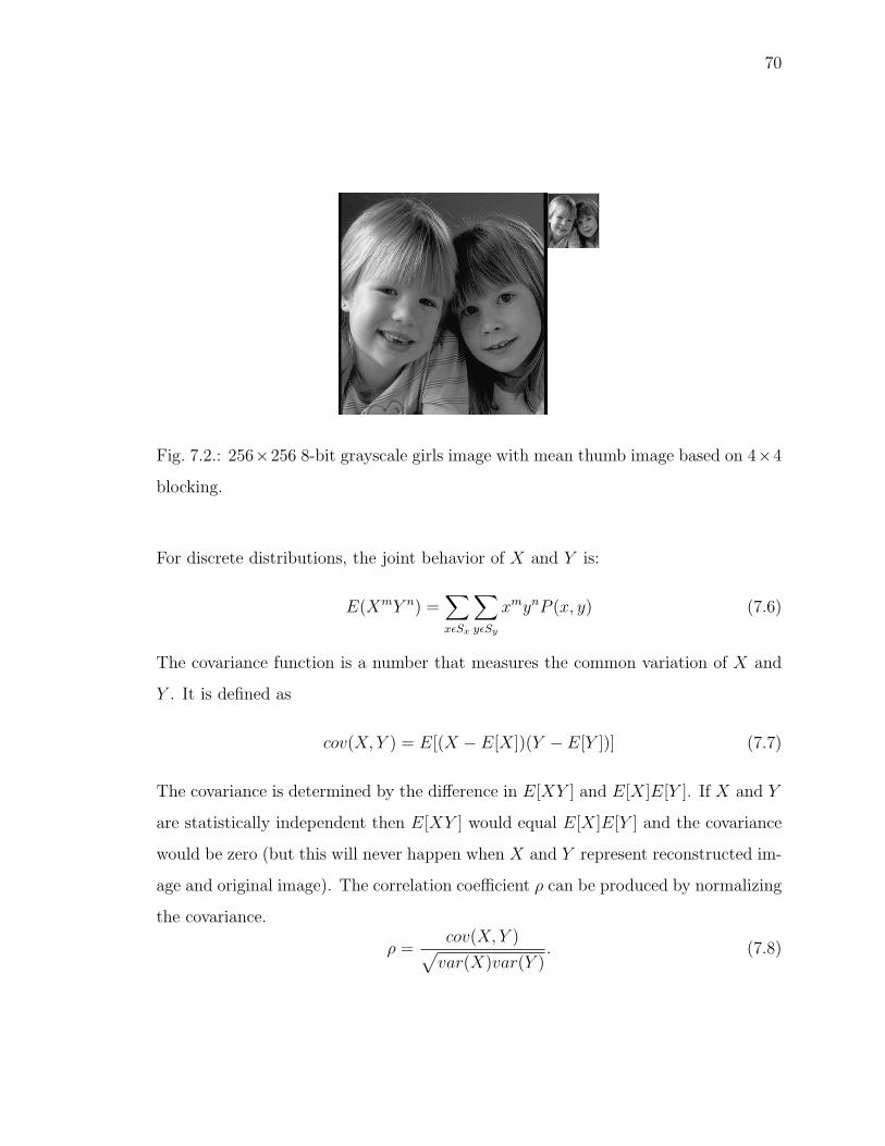
70

Fig. 7.2.: 256×256 8-bit grayscale girls image with mean thumb image based on 4×4

blocking.

For discrete distributions, the joint behavior of X and Y is:

E(XmY n) =∑xεSx

∑yεSy

xmynP (x, y) (7.6)

The covariance function is a number that measures the common variation of X and

Y . It is defined as

cov(X, Y ) = E[(X − E[X])(Y − E[Y ])] (7.7)

The covariance is determined by the difference in E[XY ] and E[X]E[Y ]. If X and Y

are statistically independent then E[XY ] would equal E[X]E[Y ] and the covariance

would be zero (but this will never happen when X and Y represent reconstructed im-

age and original image). The correlation coefficient ρ can be produced by normalizing

the covariance.

ρ =cov(X, Y )√var(X)var(Y )

. (7.8)

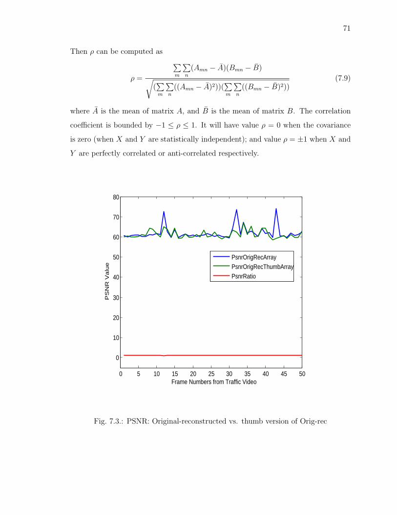
71

Then ρ can be computed as

ρ =

∑m

∑n

(Amn − A)(Bmn − B)√(∑m

∑n

((Amn − A)2))(∑m

∑n

((Bmn − B)2))(7.9)

where A is the mean of matrix A, and B is the mean of matrix B. The correlation

coefficient is bounded by −1 ≤ ρ ≤ 1. It will have value ρ = 0 when the covariance

is zero (when X and Y are statistically independent); and value ρ = ±1 when X and

Y are perfectly correlated or anti-correlated respectively.

0 5 10 15 20 25 30 35 40 45 50

0

10

20

30

40

50

60

70

80

Frame Numbers from Traffic Video

PS

NR

Valu

e

PsnrOrigRecArrayPsnrOrigRecThumbArrayPsnrRatio

Fig. 7.3.: PSNR: Original-reconstructed vs. thumb version of Orig-rec

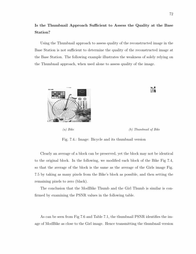
72

Is the Thumbnail Approach Sufficient to Assess the Quality at the Base

Station?

Using the Thumbnail approach to assess quality of the reconstructed image in the

Base Station is not sufficient to determine the quality of the reconstructed image at

the Base Station. The following example illustrates the weakness of solely relying on

the Thumbnail approach, when used alone to assess quality of the image.

H image

(a) Bike

H mean image

(b) Thumbnail of Bike

Fig. 7.4.: Image: Bicycle and its thumbnail version

Clearly an average of a block can be preserved, yet the block may not be identical

to the original block. In the following, we modified each block of the Bike Fig 7.4,

so that the average of the block is the same as the average of the Girls image Fig.

7.5 by taking as many pixels from the Bike’s block as possible, and then setting the

remaining pixels to zero (black).

The conclusion that the ModBike Thumb and the Girl Thumb is similar is con-

firmed by examining the PSNR values in the following table.

As can be seen from Fig 7.6 and Table 7.1, the thumbnail PSNR identifies the im-

age of ModBike as close to the Girl image. Hence transmitting the thumbnail version

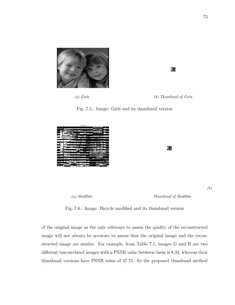
73

(a) Girls

G mean image

(b) Thumbnail of Girls

Fig. 7.5.: Image: Girls and its thumbnail version

B image

(a) ModBike

B mean image

(b)

Thumbnail of ModBike

Fig. 7.6.: Image: Bicycle modified and its thumbnail version

of the original image as the only reference to assess the quality of the reconstructed

image will not always be accurate to assess that the original image and the recon-

structed image are similar. For example, from Table 7.1, images G and B are two

different/uncorrelated images with a PSNR value between them is 8.33, whereas their

thumbnail versions have PSNR value of 37.75. So the proposed thumbnail method

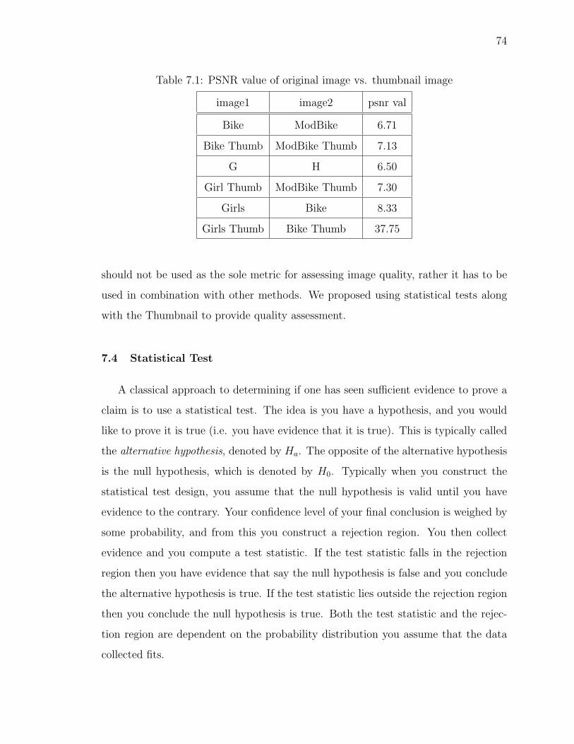
74

Table 7.1: PSNR value of original image vs. thumbnail image

image1 image2 psnr val

Bike ModBike 6.71

Bike Thumb ModBike Thumb 7.13

G H 6.50

Girl Thumb ModBike Thumb 7.30

Girls Bike 8.33

Girls Thumb Bike Thumb 37.75

should not be used as the sole metric for assessing image quality, rather it has to be

used in combination with other methods. We proposed using statistical tests along

with the Thumbnail to provide quality assessment.

7.4 Statistical Test

A classical approach to determining if one has seen sufficient evidence to prove a

claim is to use a statistical test. The idea is you have a hypothesis, and you would

like to prove it is true (i.e. you have evidence that it is true). This is typically called

the alternative hypothesis, denoted by Ha. The opposite of the alternative hypothesis

is the null hypothesis, which is denoted by H0. Typically when you construct the

statistical test design, you assume that the null hypothesis is valid until you have

evidence to the contrary. Your confidence level of your final conclusion is weighed by

some probability, and from this you construct a rejection region. You then collect

evidence and you compute a test statistic. If the test statistic falls in the rejection

region then you have evidence that say the null hypothesis is false and you conclude

the alternative hypothesis is true. If the test statistic lies outside the rejection region

then you conclude the null hypothesis is true. Both the test statistic and the rejec-

tion region are dependent on the probability distribution you assume that the data

collected fits.

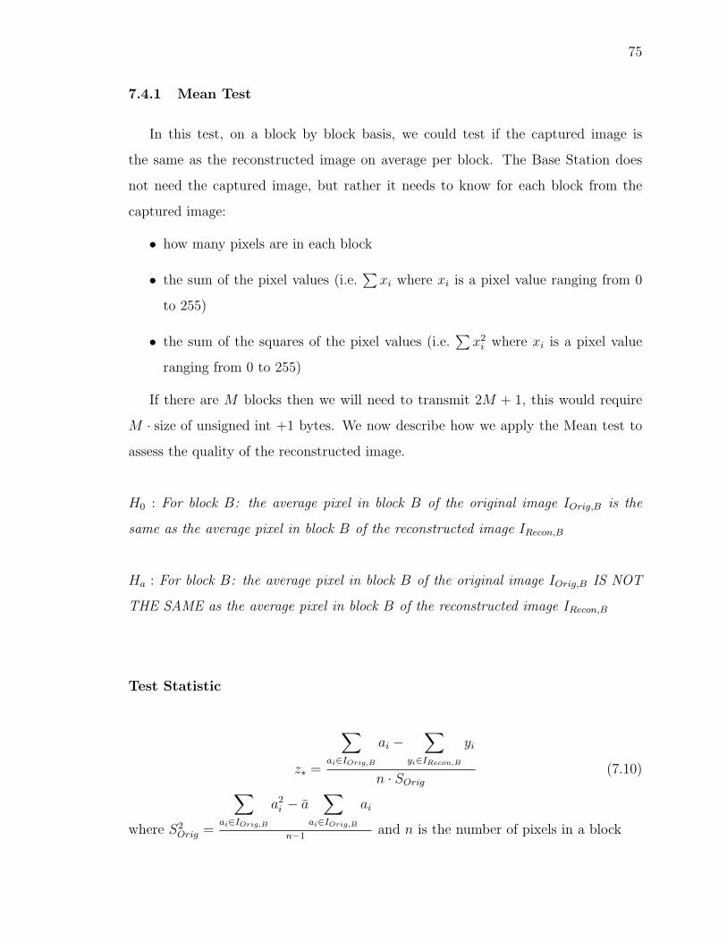
75

7.4.1 Mean Test

In this test, on a block by block basis, we could test if the captured image is

the same as the reconstructed image on average per block. The Base Station does

not need the captured image, but rather it needs to know for each block from the

captured image:

• how many pixels are in each block

• the sum of the pixel values (i.e.∑xi where xi is a pixel value ranging from 0

to 255)

• the sum of the squares of the pixel values (i.e.∑x2i where xi is a pixel value

ranging from 0 to 255)

If there are M blocks then we will need to transmit 2M + 1, this would require

M · size of unsigned int +1 bytes. We now describe how we apply the Mean test to

assess the quality of the reconstructed image.

H0 : For block B: the average pixel in block B of the original image IOrig,B is the

same as the average pixel in block B of the reconstructed image IRecon,B

Ha : For block B: the average pixel in block B of the original image IOrig,B IS NOT

THE SAME as the average pixel in block B of the reconstructed image IRecon,B

Test Statistic

z∗ =

∑ai∈IOrig,B

ai −∑

yi∈IRecon,B

yi

n · SOrig(7.10)

where S2Orig =

∑ai∈IOrig,B

a2i − a

∑ai∈IOrig,B

ai

n−1and n is the number of pixels in a block

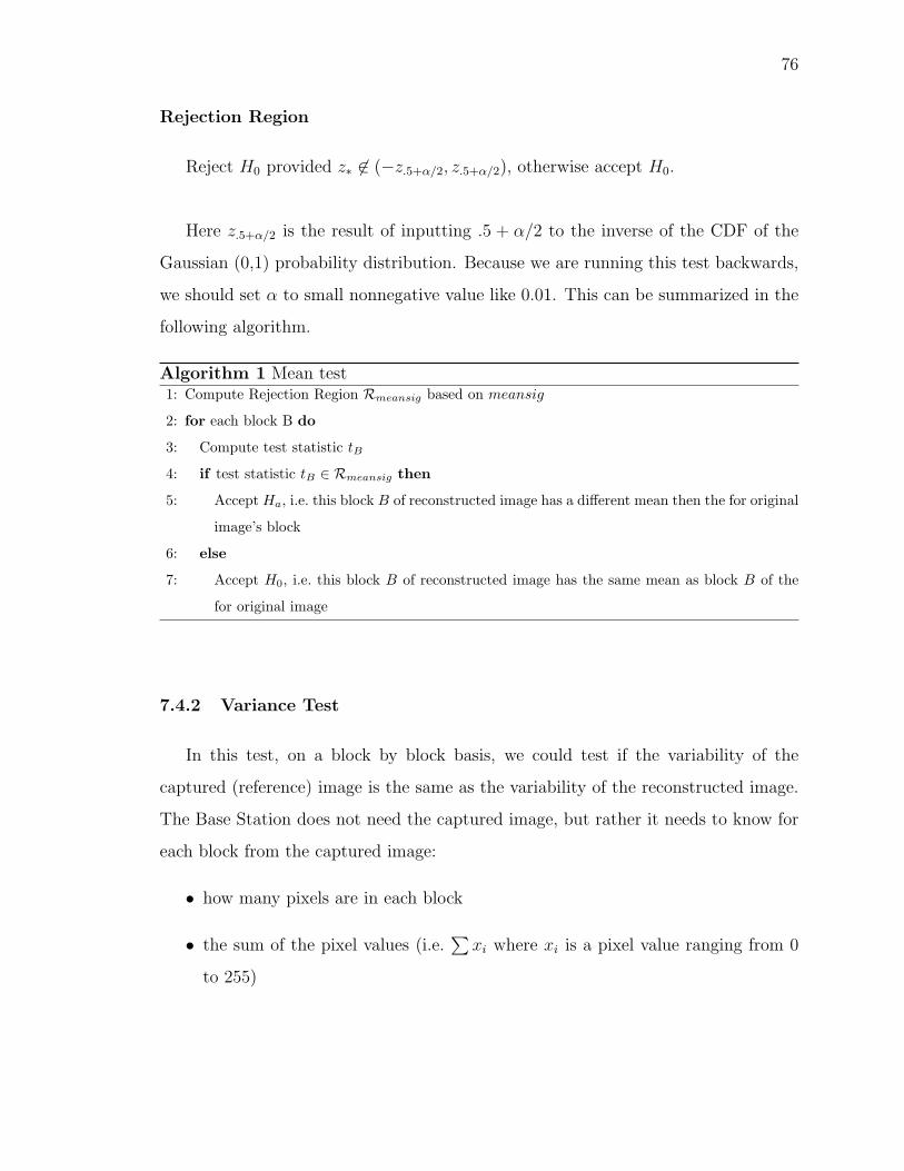
76

Rejection Region

Reject H0 provided z∗ 6∈ (−z.5+α/2, z.5+α/2), otherwise accept H0.

Here z.5+α/2 is the result of inputting .5 + α/2 to the inverse of the CDF of the

Gaussian (0,1) probability distribution. Because we are running this test backwards,

we should set α to small nonnegative value like 0.01. This can be summarized in the

following algorithm.

Algorithm 1 Mean test1: Compute Rejection Region Rmeansig based on meansig

2: for each block B do

3: Compute test statistic tB

4: if test statistic tB ∈ Rmeansig then

5: Accept Ha, i.e. this block B of reconstructed image has a different mean then the for original

image’s block

6: else

7: Accept H0, i.e. this block B of reconstructed image has the same mean as block B of the

for original image

7.4.2 Variance Test

In this test, on a block by block basis, we could test if the variability of the

captured (reference) image is the same as the variability of the reconstructed image.

The Base Station does not need the captured image, but rather it needs to know for

each block from the captured image:

• how many pixels are in each block

• the sum of the pixel values (i.e.∑xi where xi is a pixel value ranging from 0

to 255)

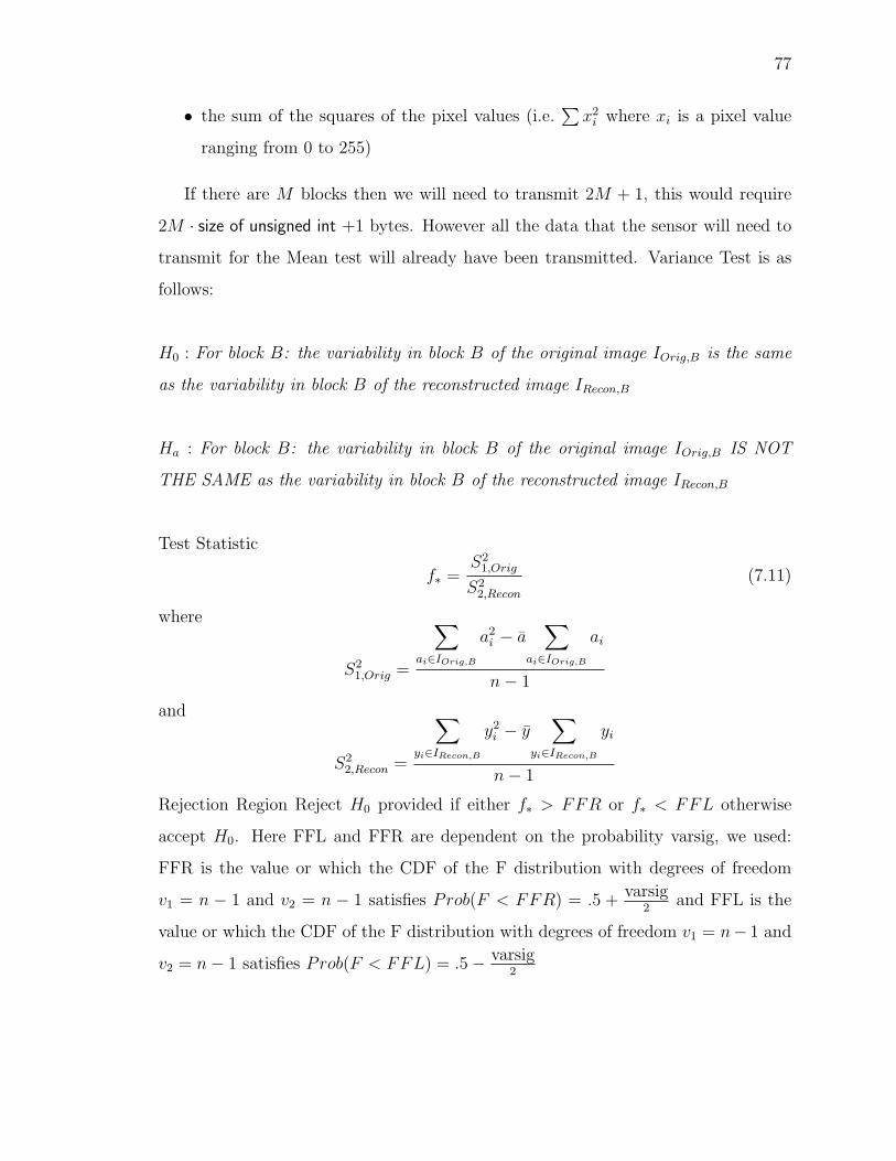
77

• the sum of the squares of the pixel values (i.e.∑x2i where xi is a pixel value

ranging from 0 to 255)

If there are M blocks then we will need to transmit 2M + 1, this would require

2M · size of unsigned int +1 bytes. However all the data that the sensor will need to

transmit for the Mean test will already have been transmitted. Variance Test is as

follows:

H0 : For block B: the variability in block B of the original image IOrig,B is the same

as the variability in block B of the reconstructed image IRecon,B

Ha : For block B: the variability in block B of the original image IOrig,B IS NOT

THE SAME as the variability in block B of the reconstructed image IRecon,B

Test Statistic

f∗ =S2

1,Orig

S22,Recon

(7.11)

where

S21,Orig =

∑ai∈IOrig,B

a2i − a

∑ai∈IOrig,B

ai

n− 1

and

S22,Recon =

∑yi∈IRecon,B

y2i − y

∑yi∈IRecon,B

yi

n− 1

Rejection Region Reject H0 provided if either f∗ > FFR or f∗ < FFL otherwise

accept H0. Here FFL and FFR are dependent on the probability varsig, we used:

FFR is the value or which the CDF of the F distribution with degrees of freedom

v1 = n − 1 and v2 = n − 1 satisfies Prob(F < FFR) = .5 +varsig

2and FFL is the

value or which the CDF of the F distribution with degrees of freedom v1 = n− 1 and

v2 = n− 1 satisfies Prob(F < FFL) = .5− varsig2

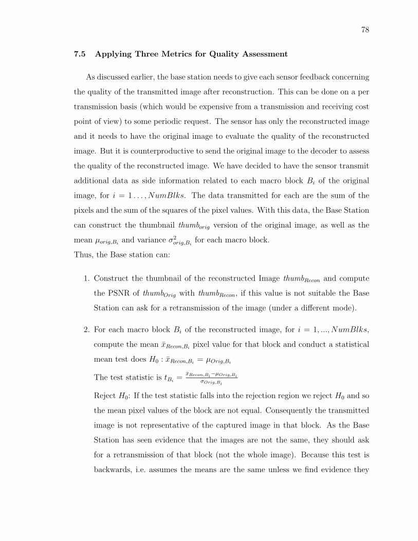
78

7.5 Applying Three Metrics for Quality Assessment

As discussed earlier, the base station needs to give each sensor feedback concerning

the quality of the transmitted image after reconstruction. This can be done on a per

transmission basis (which would be expensive from a transmission and receiving cost

point of view) to some periodic request. The sensor has only the reconstructed image

and it needs to have the original image to evaluate the quality of the reconstructed

image. But it is counterproductive to send the original image to the decoder to assess

the quality of the reconstructed image. We have decided to have the sensor transmit

additional data as side information related to each macro block Bi of the original

image, for i = 1 . . . , NumBlks. The data transmitted for each are the sum of the

pixels and the sum of the squares of the pixel values. With this data, the Base Station

can construct the thumbnail thumborig version of the original image, as well as the

mean µorig,Biand variance σ2

orig,Bifor each macro block.

Thus, the Base station can:

1. Construct the thumbnail of the reconstructed Image thumbRecon and compute

the PSNR of thumbOrig with thumbRecon, if this value is not suitable the Base

Station can ask for a retransmission of the image (under a different mode).

2. For each macro block Bi of the reconstructed image, for i = 1, ..., NumBlks,

compute the mean xRecon,Bipixel value for that block and conduct a statistical

mean test does H0 : xRecon,Bi= µOrig,Bi

The test statistic is tBi=

xRecon,Bi−µOrig,Bi

σOrig,Bi

Reject H0: If the test statistic falls into the rejection region we reject H0 and so

the mean pixel values of the block are not equal. Consequently the transmitted

image is not representative of the captured image in that block. As the Base

Station has seen evidence that the images are not the same, they should ask

for a retransmission of that block (not the whole image). Because this test is

backwards, i.e. assumes the means are the same unless we find evidence they

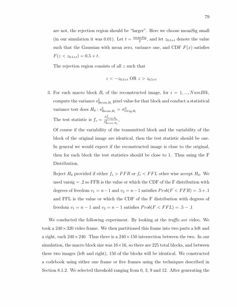
79

are not, the rejection region should be “larger”. Here we choose meanSig small

(in our simulation it was 0.01). Let t = meanSig2

, and let z0.5+t denote the value

such that the Gaussian with mean zero, variance one, and CDF F (x) satisfies

F (z < z0.5+t) = 0.5 + t.

The rejection region consists of all z such that

z < −z0.5+t OR z > z0.5+t

3. For each macro block Bi of the reconstructed image, for i = 1, ..., NumBlk,

compute the variance s2Recon,Bi

pixel value for that block and conduct a statistical

variance test does H0 : s2Recon,Bi

= σ2Orig,Bi

The test statistic is f∗ =σ2

Orig,Bi

s2Recon,Bi

,

Of course if the variability of the transmitted block and the variability of the

block of the original image are identical, then the test statistic should be one.

In general we would expect if the reconstructed image is close to the original,

then for each block the test statistics should be close to 1. Thus using the F

Distribution.

Reject H0 provided if either f∗ > FFR or f∗ < FFL other wise accept H0. We

used varsig = .2 so FFR is the value or which the CDF of the F distribution with

degrees of freedom v1 = n−1 and v2 = n−1 satisfies Prob(F < FFR) = .5+ .1

and FFL is the value or which the CDF of the F distribution with degrees of

freedom v1 = n− 1 and v2 = n− 1 satisfies Prob(F < FFL) = .5− .1

We conducted the following experiment. By looking at the traffic.avi video. We

took a 240×320 video frame. We then partitioned this frame into two parts a left and

a right, each 240×240. Thus there is a 240×150 intersection between the two. In our

simulation, the macro block size was 16×16, so there are 225 total blocks, and between

these two images (left and right), 150 of the blocks will be identical. We constructed

a codebook using either one frame or five frames using the techniques described in

Section 8.1.2. We selected threshold ranging from 0, 3, 9 and 12. After generating the

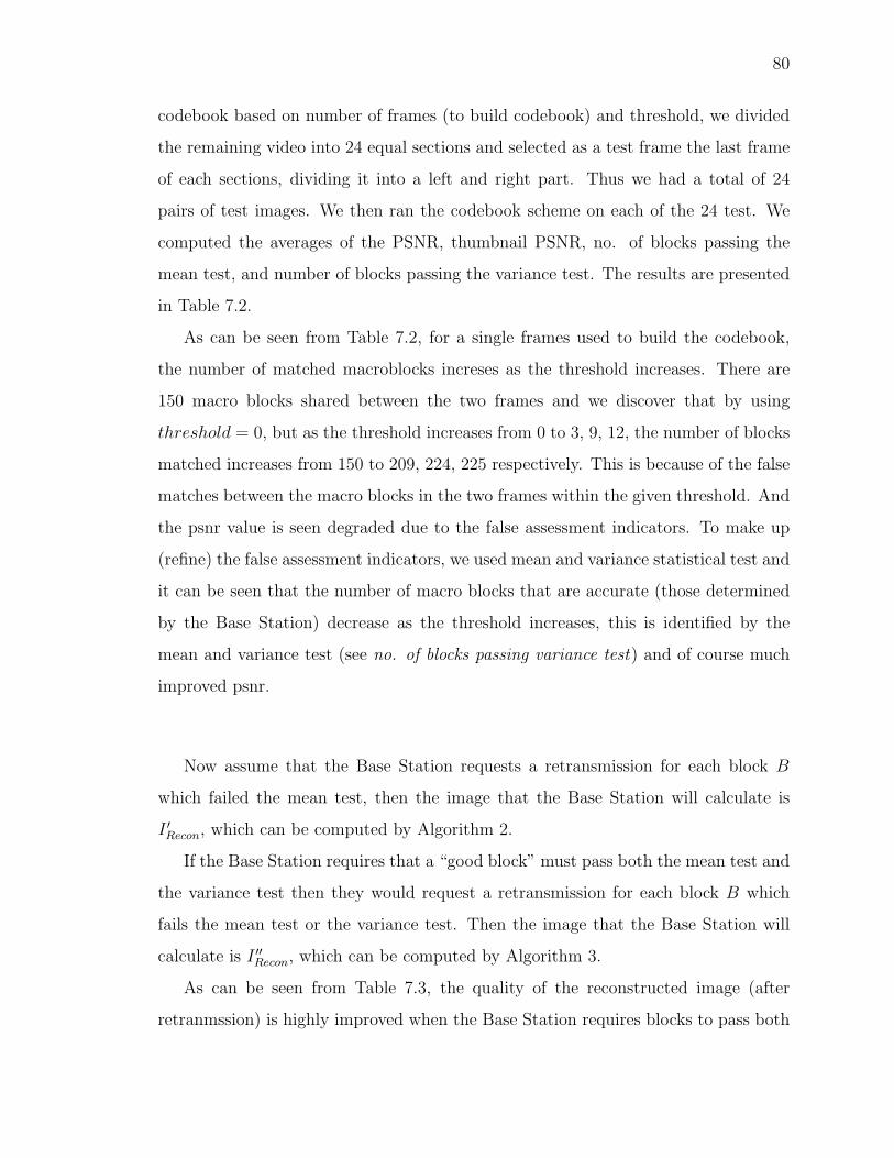
80

codebook based on number of frames (to build codebook) and threshold, we divided

the remaining video into 24 equal sections and selected as a test frame the last frame

of each sections, dividing it into a left and right part. Thus we had a total of 24

pairs of test images. We then ran the codebook scheme on each of the 24 test. We

computed the averages of the PSNR, thumbnail PSNR, no. of blocks passing the

mean test, and number of blocks passing the variance test. The results are presented

in Table 7.2.

As can be seen from Table 7.2, for a single frames used to build the codebook,

the number of matched macroblocks increses as the threshold increases. There are

150 macro blocks shared between the two frames and we discover that by using

threshold = 0, but as the threshold increases from 0 to 3, 9, 12, the number of blocks

matched increases from 150 to 209, 224, 225 respectively. This is because of the false

matches between the macro blocks in the two frames within the given threshold. And

the psnr value is seen degraded due to the false assessment indicators. To make up

(refine) the false assessment indicators, we used mean and variance statistical test and

it can be seen that the number of macro blocks that are accurate (those determined

by the Base Station) decrease as the threshold increases, this is identified by the

mean and variance test (see no. of blocks passing variance test) and of course much

improved psnr.

Now assume that the Base Station requests a retransmission for each block B

which failed the mean test, then the image that the Base Station will calculate is

I ′Recon, which can be computed by Algorithm 2.

If the Base Station requires that a “good block” must pass both the mean test and

the variance test then they would request a retransmission for each block B which

fails the mean test or the variance test. Then the image that the Base Station will

calculate is I ′′Recon, which can be computed by Algorithm 3.

As can be seen from Table 7.3, the quality of the reconstructed image (after

retranmssion) is highly improved when the Base Station requires blocks to pass both

81

Table 7.2: Codebook results on traffic.avi video

Threshold No. (frames) No. PSNR Thumbnail No. (blocks) No. (blocks)

to build blocks in PSNR passing passing

Codebook Codebook Mean Variance

Test Test

0 1 150 Inf Inf 225 225

3 1 209 15.598 19.936 69.958 74.5

9 1 224 13.24 17.288 23.458 28.541

12 1 225 12.165 15.780 15.750 20.041

9 5 35 39.333 44.9977 201.5 203.9

Algorithm 2 Computing I ′Recon1: for each block B do

2: if IRecon,B with test statistic tB passes Mean Test with rejection region Rmeansig then

3: I ′Recon,B = IRecon,B

4: else

5: I ′Recon,B = IOrig,B

Algorithm 3 Quality assessment using both mean and variance test–computing

I ′′Recon1: for each block B do

2: if IRecon,B with test statistic fB passes Variance Test with rejection region Fvarsig then

3: I ′′Recon,B = I ′Recon,B

4: else

5: I ′′Recon,B = IOrig,B

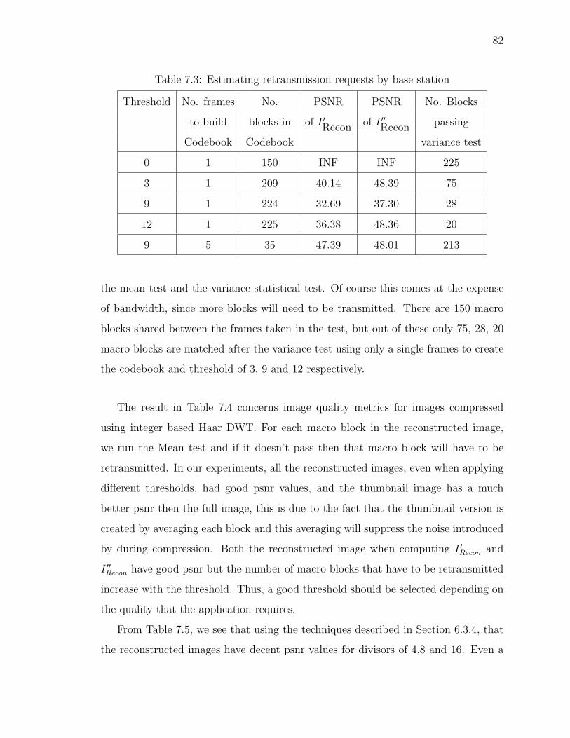
82

Table 7.3: Estimating retransmission requests by base station

Threshold No. frames No. PSNR PSNR No. Blocks

to build blocks in of I ′Recon of I ′′Recon passing

Codebook Codebook variance test

0 1 150 INF INF 225

3 1 209 40.14 48.39 75

9 1 224 32.69 37.30 28

12 1 225 36.38 48.36 20

9 5 35 47.39 48.01 213

the mean test and the variance statistical test. Of course this comes at the expense

of bandwidth, since more blocks will need to be transmitted. There are 150 macro

blocks shared between the frames taken in the test, but out of these only 75, 28, 20

macro blocks are matched after the variance test using only a single frames to create

the codebook and threshold of 3, 9 and 12 respectively.

The result in Table 7.4 concerns image quality metrics for images compressed

using integer based Haar DWT. For each macro block in the reconstructed image,

we run the Mean test and if it doesn’t pass then that macro block will have to be

retransmitted. In our experiments, all the reconstructed images, even when applying

different thresholds, had good psnr values, and the thumbnail image has a much

better psnr then the full image, this is due to the fact that the thumbnail version is

created by averaging each block and this averaging will suppress the noise introduced

by during compression. Both the reconstructed image when computing I ′Recon and

I ′′Recon have good psnr but the number of macro blocks that have to be retransmitted

increase with the threshold. Thus, a good threshold should be selected depending on

the quality that the application requires.

From Table 7.5, we see that using the techniques described in Section 6.3.4, that

the reconstructed images have decent psnr values for divisors of 4,8 and 16. Even a

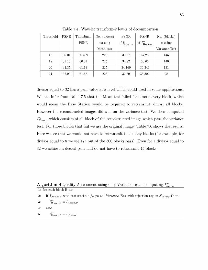
83

Table 7.4: Wavelet transform-2 levels of decomposition

Threshold PSNR Thumbnail No. (blocks) PSNR PSNR No. (blocks)

PSNR passing of I ′Recon of I ′′Recon passing

Mean test Variance Test

16 36.04 60.439 225 35.67 37.26 145

18 35.16 60.87 225 34.82 36.65 140

20 34.35 61.13 225 34.169 36.346 131

24 32.90 61.66 225 32.59 36.302 98

divisor equal to 32 has a psnr value at a level which could used in some applications.

We can infer from Table 7.5 that the Mean test failed for almost every block, which

would mean the Base Station would be required to retransmit almost all blocks.

However the reconstructed images did well on the variance test. We then computed

I ′′′Recon, which consists of all block of the reconstructed image which pass the variance

test. For those blocks that fail we use the original image. Table 7.6 shows the results.

Here we see that we would not have to retransmit that many blocks (for example, for

divisor equal to 8 we see 174 out of the 300 blocks pass). Even for a divisor equal to

32 we achieve a decent psnr and do not have to retransmit 45 blocks.

Algorithm 4 Quality Assessment using only Variance test – computing I ′′′Recon1: for each block B do

2: if IRecon,B with test statistic fB passes Variance Test with rejection region Fvarsig then

3: I ′′′Recon,B = IRecon,B

4: else

5: I ′′′Recon,B = IOrig,B

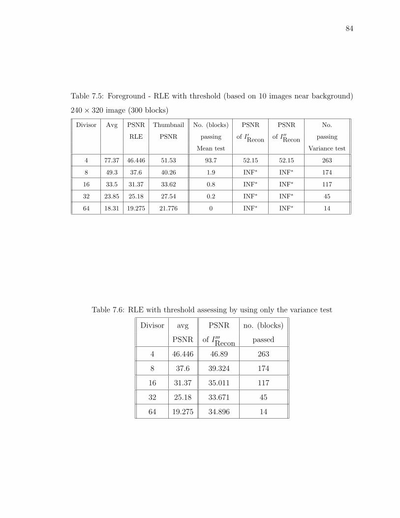
84

Table 7.5: Foreground - RLE with threshold (based on 10 images near background)

240× 320 image (300 blocks)

Divisor Avg PSNR Thumbnail No. (blocks) PSNR PSNR No.

RLE PSNR passing of I ′Recon of I ′′Recon passing

Mean test Variance test

4 77.37 46.446 51.53 93.7 52.15 52.15 263

8 49.3 37.6 40.26 1.9 INF∗ INF∗ 174

16 33.5 31.37 33.62 0.8 INF∗ INF∗ 117

32 23.85 25.18 27.54 0.2 INF∗ INF∗ 45

64 18.31 19.275 21.776 0 INF∗ INF∗ 14

Table 7.6: RLE with threshold assessing by using only the variance test

Divisor avg PSNR no. (blocks)

PSNR of I ′′′Recon passed

4 46.446 46.89 263

8 37.6 39.324 174

16 31.37 35.011 117

32 25.18 33.671 45

64 19.275 34.896 14

85

8. DECODER

We now discuss the decoder and decoding process. Recall that we have switched the

traditional complex encoder/simple decoder to a simple encoder/complex decoder by

placing some of the intensive computation on the decoder side (assuming the base

station has enough computational resources).

8.1 Decoding Packets and Coordinating Sensor Operation

The primary function of the decoder is undoing the encoding so that the original

information can be retrieved. As it discussed earlier, it is infeasible to use the existing

state-of-the-art video coding algorithms such as MPEG 2/4, H.264 etc to compress

sensor readings due to their high computational complexity.

8.1.1 Decoding Packets Received from the Sensor:

The decoding procedure is such that it will decode the bit stream received and

assimilate the data to retrieve the transmitted signal. The design of the decoder is

based on the inverse operations of the technques discussed earlier. The decoder will

appear a illustrated in Fig 8.1.

Decoding Packet Encoded using Background Subtraction Method

The decoder will read the packet header received from the sensors, and if the

packet mode was encoded using the Background Subtraction Method, the decoder

will perform the following operations to reconstruct the image. First update the

background model:

IBt+1 = αICt + (1− α)IBt .

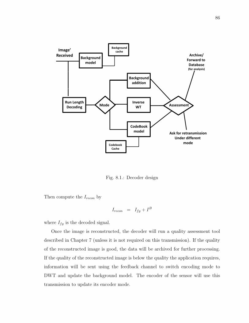
86

A hi /

BackgroundcacheImage’

R i d Backgroundmodel

Archive/Forward to Database(for analysis)

Received

Backgroundaddition

Run LengthD di

InverseWTMode AssessmentDecoding WTMode Assessment

CodeBookmodel Ask for retransmission

Under different

CodebookCache

mode

Fig. 8.1.: Decoder design

Then compute the Irecon by

Irecon = Ifg + IB

where Ifg is the decoded signal.

Once the image is reconstructed, the decoder will run a quality assessment tool

described in Chapter 7 (unless it is not required on this transmission). If the quality

of the reconstructed image is good, the data will be archived for further processing.

If the quality of the reconstructed image is below the quality the application requires,

information will be sent using the feedback channel to switch encoding mode to

DWT and update the background model. The encoder of the sensor will use this

transmission to update its encoder mode.

87

Decoding Packet Encoded Using Discrete Wavelet Transform (DWT)

If the received packets from the sensors were encoded using DWT , then the Inverse

Wavelet Transform (IWT) operation will be executed to reconstruct the original signal

from the wavelet coefficients.

The original pixel values can be reconstructed using a multilevel wavelet recon-

struction of the bitstream based on the wavelet decomposition structure from the

wavelet decomposition step. After reconstruction the quality of the reconstructed

image will be assessed (unless it is not required on this transmission) and if the qual-

ity is less than the value the application requires, the encoder will be flagged to send

more refinement bits (such as to send LH2 for an image encoded with 3 levels of

wavelet decomposition).

Decoding Packet Encoded Using Codebook

If the mode was codebook, the decoder will use the codebook ID of the neigh-

bor sensor that was used to piece together pieces transmitted by sensor and pieces

transmitted by neighbor. For the pieces transmitted by sensor they may have been

transmitted by background subtraction, wavelet transform or neither. After piecing

together the reconstructed image, the base station will assess the quality of the image

(unless it is not required on this transmission).

8.1.2 Block Matching Algorithm (BMA)

It has been widely argued, that a group of sensors performs better in the sensing

task than one powerful sensor [32]. In such a sensor network, a group of spatially

proximate sensors are very likely to have correlated readings, i.e. due to high density

in network topology, sensor observations are highly correlated in the space domain

(spatial correlation). Furthermore, the nature of the physical phenomenon constitutes

the temporal correlation between each consecutive observation of a sensor node. It is

88

important to design a good algorithm to exploit this correlation to save transmission

power on these resource constrained devices (sensors). If information covering a

certain area that’s monitored is sent by one of the neighbor sensors, the next sensor

monitoring part of that area should take advantage of its neighbor’s transmission.

The search algorithm will be computationally intensive, so the base station (decoder)

will compute the position vectors and transmit this information back to the encoder

using the feedback channel.

Exploiting Spatial/Temporal Correlation: Using Block Matching Algo-

rithm

Consider an image divided into small non-overlapping macro blocks (e.g. 16×16).

For each block in the first image the algorithm tries to find a block of the same size in

the second image that is most similar to the block in the first image within a suitably

sized search range (R). Different metrics can be used to measure similarity such as

computing the difference between blocks and use cross correlation, squared difference,

absolute difference, etc. In our experiment, the metric used for matching the macro

blocks is mean absolute difference (MAD), a small MAD implies macro blocks are

similar (with some threshold).

MAD(A,B) =1

m · n

m∑p=1

n∑q=1

[A(p, q)−B(p, q)] (8.1)

The function searches in the neighborhood of some given point in the second

image by shifting points in the block by the same offset. At each shift, the sum of

the distance between the gray values of the two macro blocks is computed. The shift

which gives the smallest distance is considered the best match. The search range and

how we measure similarity has a great effect in the block matching algorithm, i.e.

wider search range will result in the best match but at the expense of computation,

and the threshold determines how similar the two macro-blocks are. A fairly low

threshold has to be set to get less distortion between the two macro blocks since

those blocks who are discovered ”matched” by the algorithm will not be encoded

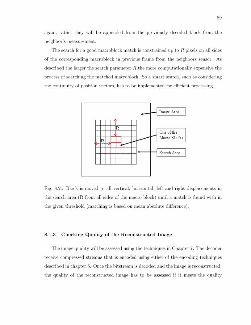
89

again, rather they will be appended from the previously decoded block from the

neighbor’s measurement.

The search for a good macroblock match is constrained up to R pixels on all sides

of the corresponding macroblock in previous frame from the neighbors sensor. As

described the larger the search parameter R the more computationally expensive the

process of searching the matched macroblock. So a smart search, such as considering

the continuity of position vectors, has to be implemented for efficient processing.

1

R

R

Fig. 8.2.: Block is moved to all vertical, horizontal, left and right displacements in

the search area (R from all sides of the macro block) until a match is found with in

the given threshold (matching is based on mean absolute difference).

8.1.3 Checking Quality of the Reconstructed Image

The image quality will be assessed using the techniques in Chapter 7. The decoder

receive compressed streams that is encoded using either of the encoding techniques

described in chapter 6. Once the bitstream is decoded and the image is reconstructed,

the quality of the reconstructed image has to be assessed if it meets the quality

90

Algorithm 5 Block Matching Algorithm (BMA) using exhaustive search with in the

search parameter

Input: mbSize, searchRange, searchIncr, Image, refImage, row, col, thresh

Output: codeBk

1: for i = 1 to row do

2: for j = 1 to col do

3: codeBk(i, j) = 0

4: for i = 1 to row −mbSize + 1 step i = i + mbSize do

5: for j = 1 to row −mbSize + 1 step i = i + mbSize do

6: FOUND = 0

7: for m = −searchRange to searchRange step m = m+searchIncr do

8: for n = −searchRange to searchRange step n = n+searchIncr do

9: if mbSize×mbSize block determined by coordinate (i+m, j +n) is entirely contained

within refImage then

10: Let cost= MeanAbsoluteDistance( Block(Image, i,j,mbSize), Block(refImage,

i+m,j+n,mbSize))

11: if cost ≤ thresh then

12: codeBk(i, j) = i + m + row · (j + n)

13: FOUND=1

14: break

15: if FOUND = 1 then

16: break

91

required by the application. For example, if the application is for surveillance, a little

more lossy is tolerable.

As discussed earlier we will use Reduced-Reference (RR) quality assessment meth-

ods in which partial information regarding the ’perfect version’ is available. Formally,

a side-channel (called an RR channel) exists through which some information regard-

ing the reference can be made available to the QA algorithm. RR QA algorithms use

this partial reference information to judge the quality of the reconstructed signal.

Image thumbnail as a side information, as described in Section 7.3.1, the image

thumbnail is created after partitioning the image in to square blocks of pixels in which

a single mean value representing each block. There is an inverse proportionality be-

tween the size of each macroblock and the how close the thumbnail image represent

the reference image. A single mean value representing each block will create the

thumbnail version of the reference image and this thumbnail version will be sent to

the decoder using the side channel. The decoder will reconstruct the image from

the bitstreams received from each sensor and create thumbnail version of the recon-

structed image using same procedure above. The thumbnail version of the original

and reconstructed will be can be used to computer the standard quality assessment

tools as MSE or PSNR. As can be seen in Figure 7.3 in Chapter 7, there is a high

correlation (almost identical) between reference image and its reconstructed version

and their thumbnail version.

Mean and Variance hypothesis test, Since we do not have the reference image at

the decoder side to evaluate the quality of the reconstructed image, we have proposed

to use both a mean and variance hypothesis test using side information from the

encoder. This method is described in Chapter 7.

92

9. CONCLUSION AND FUTURE WORK

Conclusion:

In this thesis we have constructed a full codec for lightweight encoding for de-

vices with resource constraints like wireless sensor networks, PDA, etc. The codec

is designed targeting applications that tolerates a bit more loss of information dur-

ing source coding than MPEG 2/4 or H.264, like surveillance applications. We also

showed the insecurity of wavelet tree shuffling scheme as the only security mechanism

in multimedia encryption and propose it as a supplementary security mechanism.

In Chapter 34, we have reviewed selective encryption on wavelet based compression

techniques and assessed the security of some of the proposed selective encryption

algorithms. Specifically we have assessed the algorithm proposed by Kwon et. al. [5]

for selectively encrypting the content of video file for digital rights management. We

showed the flaw of the design and suggest that wavelet tree shuffling will not give the

desired security if it is used as the only security mechanism.

In Chapter 5, we have provided the overall design of the codec. We also provide

the metrics that we used in the subsequent chapters to evaluate the performance of

our codec design.

In Chapter 6, we have discussed and provided encoding system in which it can

be optimized to the level the application requires. The encoding system will switch

between three compression modes (DWT, background subtraction and codebook) for

efficient operation. We have used integer based Haar wavelets for efficient operation

in resource constrained devices, and simple differencing between a background model

representing the static scene of each sensor camera. We have suggested a quantization

scheme to encode each pixel during run length encoding of the foreground image. In

addition, we have suggested a block matching algorithm to exploit the spatial corre-

lation between proximate sensor reading. Searching of a match in a block matching

93

algorithm very intensive computation and it is infeasible to implement the algorithm

in sensor nodes. Thus, we have switched the traditional encoding order complex en-

coder simple decoder to simple encoder to complex decoder (assuming the decoder in

the base station side has enough computation resources).

In Chapter 7, we have proposed different Reduced-Reference (RR) image quality

assessment tools to evaluate the quality of the reconstructed image in the decoder

side without having the original image. We have proposed sending the scaled version

(mean of each macroblock) of each frame as a side information and scaling the re-

constructed image using same procedure to assess quality of the reconstructed image.

We have found this method by itself is not sufficient to assess quality and we have

added statistical test (Mean and Variance test) to supplement the previous method.

In Chapter 8, We have described the decoding of bitstream encoded using the

different source coding techniques proposed in the the encoding system. Most of the

decoding is just the reverse operation of the encoding.

Future Work: All our results here are either theoretical analysis (counting clock

cycles) and simulations using MatLab. In future work it has to be implemented

in sensors and gather real time data for analysis. The block matching algorithm

we proposed for exploiting correlated readings between sensors is computationally

intensive. Although the Base Station is assumed to have sufficient computational

resources, the block matching algorithm has to be developed to be more for efficiency.

An exhaustive analysis of the parameter choices should be made for algorithms we

have developed to provide more intuition as to what threshold levels should be set for

what type of surveillance images and what the necessary significant levels to provide

quality assessment.

In this work we only work on the signal processing algorithm and in future work

the network protocol has also be studied and designed well to prolong the life time

of the network/devise.

LIST OF REFERENCES

94

LIST OF REFERENCES

[1] “Recommendation for Key Management,” Special Publication 800-57 Part 1,NIST, 03/2007.

[2] Keylength - Cryptographic Key Length Recommendation.http://www.keylength.com.

[3] R. Cramer and V. Shoup, “A Practical Public Key Cryptosystem ProvablySecure against Adaptive Chosen Ciphertext Attack,” In Advances in Cryptology– CRYPTO ’98 proceedings, 1998, pp. 13-25.

[4] B. Furht and D. Kirovski, Eds. Multimedia Security Handbook, CRC Press,2004.

[5] G. Kwon, T. Lee, K. Kim, J.. Jin, and S. Ko, “Multimedia digital right manage-ment using selective scrambling for mobile handset,” Computational Intelligenceand Security, LNAI, vol. 3802, pp. 1098-1103, 2005.

[6] W. Li, “Overview of Fine Granularity Scalability in MPEG-4 Video Standard,”IEEE Trans. on Circuits & Systems for Video Technology, vol.11, no.3, pp.301-317, March 2001.

[7] A. Massoudi, F. Lefebvre, C. De Vleeschouwer, B. Macq, B. and J. Quisquater,“Overview on selective encryption of image and video: challenges and perspec-tives,” EURASIP J. Inf. Security, pp. 1-18, 2008.

[8] Y. Mao and M. Wu, “A joint signal processing and cryptographic approachto multimedia encryption,” IEEE Trans. Image Processing, 15 (7) (2006), pp.2061-2075.

[9] R. Norcen and A. Uhl, “Encryption of wavelet-coded imagery using randompermutations,” in Proceedings of the IEEE International Conference on ImageProcessing (ICIP04), (Singapore), IEEE Signal Processing Society, Oct. 2004.

[10] M. Podesser, H. Schmidt, and A. Uhl, “Selective bitplane encryption for securetransmission of image data in mobile environments,” In Proceedings of the 5thNordic Signal Processing Symposium (NORSIG 02), 2002.

[11] A. Pommer and A. Uhl, “Selective encryption of wavelet-packet encoded imagedata: efficiency and security”, Multimedia Systems, vol. 9, no. 3, pp. 279-287,2003.

[12] A. Said and W.A. Pearlman, “A new, fast and efficient image codec based onset partitioning in hierarchical trees,” In IEEE Trans. Circuits and Systems forVideo Technology, volume 6(3), pp. 243-250, June 1996.

95

[13] P. Salama and B. King, “Efficient secure image transmission: compression in-tegrated with encryption,” Proc. SPIE., Vol. SPIE-5681, pp. 47-58, 2005

[14] M. Shapiro, “Embedded Image Coding using Zerotrees of Wavelet Coefficients,”IEEE Trans. Signal Processing, Vol. 41, pp. 3445-3462, 1993.

[15] A. Shamir, “How to share a secret,” Comm of ACM, vol. 22, no. 11, pp. 612-613,November 1979.

[16] D. Stinson, Cryptography: theory and practice, 2nd ed., CRC Press, 2002.

[17] T. Uehara, R. Safavi-Naini, and P. Ogunbona, “Securing wavelet compressionwith random permutations,” in Proceedings of the 2000 IEEE Pacific Rim Con-ference on Multimedia, Sydney, Dec. 2000, pp. 332-335, IEEE Signal ProcessingSociety.

[18] Z. Wang, Alan C. Bovik, Hamid Rahim Sheikh, Eero P. Simoncelli, “ImageQuality Assessment: From Error Visibility to Structural Similarity,” in IEEETRANSACTIONS ON IMAGE PROCESSING VOL. 13, NO. 4, APRIL 2004

[19] H. R. Sheikh, A. C. Bovik, and L. K. Cormack, “No-Reference Quality Assess-ment Using Natural Scene Statistics: JPEG2000,” in IEEE Transactions onImage Processing Vol. 14, No. 12, December 2005.

[20] K. Hasan and K. HaradaII, “Haar Wavelet Based Approach for Image Compres-sion and Quality Assessment of Compressed Image,” in IAENG InternationalJournal of Applied Mathematics

[21] A. Gersho and R. M. Gray, “Vector Quantization and Signal Compression,”Kluwer Academic Publishers, 1991.

[22] M. Nelson, The Data Compression Book, 2nd edi-tion., M&T books,November.1995, As appeared inhttp://www1.fatbrain.com/asp/bookinfo/bookinfo.asp?theisbn=1558514341

[23] K. Veeraraghavan, D. Peng, and H. Sharif, “Energy efficient multiresolutionvisual surveillance on wireless sensor networks,” in IEEE International Con-ference on Electro Information Technology, Lincoln, NE, 22-25 May 2005, p. 6pp.

[24] R.C. Gonzalez and R.E. Woods, “Digital Image Processing,” Pearson Educa-tion, 2003, Chapter 7 - Wavelets and Multiresolution Processing, pp. 349-394.

[25] A. Wang, W. R. Heinzelman, A. Sinha, and A. Chandrakasan, “Energy-scalableprotocols for battery-operated microsensor networks,” J. VLSI Signal Process-ing, pp. 223-237, Nov. 2001.

[26] A. Wang, A. Chandrakasan, “Energy-efficient DSPs for wireless sensor net-works,” in Signal Processing Magazine, IEEE, Volume: 19 , Issue: 4

[27] M. Ettus, “System capacity, latency and power consumption in multihop-routedSS-CDMA wireless networks,” in Proc. Radio and Wireless Conference (RAW-CON 98), Aug. 1998, pp. 55-58.

96

[28] TMS320C67x CPU and Instruction Set Reference Guide, TMS320C6000 DSPPlatform, Texas Instruments, Oct 2000, pp. 4.1-4.89, Literature Number:SPRU189F.

[29] L. Liu, Z. Li, E. J. Delp, “Efficient and Low-Complexity Surveillance VideoCompression Using Backward Channel Aware Wyner-Ziv Video Coding,” InIEEE Trans. on Circuits and Systems for Video Technology, volume 19(4), pp.453-465, April 2009.

[30] M . Srivastava, “Energy efficient wireless systems,” inSubmitted for publicationin DIMACS Summer School on Foundations of Wireless Networks and Appli-cations, August 2000 .

[31] G.J. Pottie, W.J. Kaiser, “Wireless Integrated Network Sensors,” in Comm.ACM, vol. 43, no. 5, pp. 51-58, May 2000.

[32] S. K. Jayaweera, R. Viswanathan, “Distributed Signal Processing in WirelessSensor Networks,” in IEEE Communication Letters, Vol. 9, pp. 769-771, Sept.2005.

[33] M. C. Vuran, O. B. Akan, I. F. Akyildiz, “Spatio-temporal correlation:theory and applications for wireless sensor networks,” As appeared inhttp://www.elsevier.com/locate/comnet

[34] B. Girod, A. Aaron, S. Rane, D. Rebollo-Monedero, “Distributed video coding,”Proc. IEEE 93 (1) (2005) 7183.

[35] M. Tahir and R. Farrell,“Optimal communication-computation tradeoff forwireless multimedia sensor network lifetime maximization,” in Proceedings ofthe 2009 IEEE conference on Wireless Communications & Networking Confer-ence, isbn = 978-1-4244-2947-9, 2009, 2514–2519.

[36] V. Raghunathan, C. Schurgers, S. Park, and M. B. Srivastava, “Energy AwareWireless Sensor Networks,” in IEEE Signal Processing Magazine, 19(2):4050,2002.

[37] D. Estrin and R. Govindan, “Next century challenges: scalable coordination insensor networks,” in Proc. Mobicom, pp. 263-270, 1999.

[38] W. Heinzelman, A. Chandrakasan, and H. Balakrishnan, “Energyefficient com-munication protocol for wireless sensor networks,” in Proc. Hawaii Intl. Conf.on System Sciences, Hawaii, 2000.

[39] C. Schurgers and M. Srivastava, “Energy efficient routing in sensor networks,”in Proc. Milcom, 2001.

[40] C. Wren, A. Azarhayejani, T. Darrell, and A.P. Pentland, “Pfinder: real-timetracking of the human body,” in IEEE Trans. on Patfern Anal. and MachineInfell., vol. 19, no. 7, pp. 78g785, 1997.

[41] B.P.L. Lo and S.A. Velastin, “Automatic congestion detection system for un-derground platforms,” in Proc.ISIMP2001, pp. 158-161, May2001.

[42] R. Cucchiara, C. Grana, M. Piccardi, and A. Prati, “Detecting moving objects,ghosts, and shadows in video streams,” in IEEE Tran. on Pattern Anal. andMachine Intell., vol. 25, no. 10, pp. 1337-1442,2003

97

[43] C. Stauffer and W.E.L. Grimson, “Adaptive background mixture models forreal-time tracking,” in Proc. IEEE CVPR 1999, pp. 246-252, June 1999.

[44] S. G. Mallat, “A Theory for Multiresolution Signal Decomposition: A WaveletRepresentation,” in IEEE Transactions on Pattern Analysis and Machine In-telligence, Vol 11, No. 7, July 1989.

[45] E. J. Stollnitz, T. D. DeRose, D. H. Salesin, “Wavelets for Computer Graphics:A Primer Part I,” in IEEE Computer Graphics and Applications, 15, May 1995.

[46] J. S. Walker, A Premier on Wavelets and Their Scientific Applications. Chap-man & Hall, 2008.

[47] A. Papoulis, S. U. Pillai, Probability, Random Variables and Stochastic Pro-cesses. Mc Graw Hill, Fourth Edition.

[48] A. Elgammal, R. Duraiswami, D. Harwood, and L. S. Davis“Background andforeground modeling using nonparametric kernel density estimation for visualsurveillance,” in Proceedings of the IEEE, 90(7):1151-1163, July 2002.

[49] J. Rymel, J. Renno, D. Greenhill, J. Orwell, G.A. Jones, “Adaptive eigen-backgrounds for object detection,” in International Conference on Image Pro-cessing, ICIP ’04, Oct. 2004, Vol. 3, 24-27 Oct.

[50] Y. Yu, V. K. Prassana, B. Krishnamachari, V.K Kumar, “Information Process-ing and Routing in Wireless Sensor Networks,” World Scientific Publishing Co.Pte. Ltd, 2006.

[51] I.F Akyildiz, W. SU, Y. Sankarasubramaniam, E. Cayirci, “Wireless SensorNetworks: a survey,” in Computer Networks, 38, pp. 393-422, 2002.

[52] A. Perrig, J. Stankovic, D. Wagner, “Security in Wireless Sensor Networks”

[53] W. Stallings, L. Brown, Computer Security: Principles and Practice. PearsonEducation. Inc, 2008.

[54] B. Fyrht, D. Kirovski, Multimedia Security Handbook. CRC Press LLC, Decem-ber 2004.

[55] H. Kiya, D. Imaizumi, and O. Watanabe, “Partial-scrambling of images en-coded using JPEG2000 without generating marker codes,” in Proc. IEEE Int.Conference on Image Processing (ICIP2003), volume 3, pages 205208, 2003.

[56] C. Shi and B. Bhargava, “Light-weight MPEG video encryption algorithm,”in Proc. Int. Conference on Multimedia (Multimedia 98), Shaping the Future,pages 5561, 1998.

[57] B. Bhargava, C. Shi, and S.y Wang, “MPEG video encryption algorithms. Mul-timedia Tools and Applications,” 24(1):5779, 2004.

[58] M.S Kankanhalli and T. Guan, “Compressed-domain scrambler/descramblerfor digital video,” in IEEE Trans. Consumer Eletronics, 48(2):356365, 2002.

[59] W. Zeng and S. Lei, “Efficient frequency domain video scrambling for contentaccess control,” in Proc. 7th ACM Int. Conference on Multimedia, pages 285294,1999.

98

[60] A. Uhl and A. Pommer, Image and Video Encryption: From Digital RightsManagement to Secured Personal Communication. Boston: Springer, 2005.

[61] S. Jalal, B. King, “An Anonymous Authentication Protocol: Acieving Provacywith Trust,” MSc Thesis, Purdue University, Indianapolis.

[62] A. Eskicioglu and E. J. Delp, “An Integrated Approach To Encrypting ScalableVideo,” in Proceedings of the IEEE International Conference on Multimediaand Expo, August 26-29, 2002, Lausanne, Switzerland

[63] R. B. Wolfgang and E. J. Delp, “Overview of Image Security Techniques withApplications in Multimedia Systems,” in Proceedings of the SPIE Conference onMultimedia Networks: Security, Displays, Terminals, and Gatweys, Vol. 3228,November 2-5, 1997, Dallas, Texas, pp. 297-308

[64] M. Eskicioglu, J. Town, and E. J. Delp, “Security of Digital EntertainmentContent from Creation to Consumption,” in Proceedings of the SPIE Conferenceon Applications of Digital Image Processing XXIV, Vol. 4472, San Diego, July2001, pp. 187-211

[65] M. Eskicioglu and E. J. Delp, “An Overview of Multimedia Content Protectionin Consumer Electronics Devices,” in Proceedings of the SPIE InternationalConference on Security and Watermarking of Multimedia Contents II, Vol. 3971,January 23 - 28, 2000, San Jose, CA.

[66] R. B. Wolfgang and E. J. Delp, “Overview of Image Security Techniques withApplications in Multimedia Systems,” in Proceedings of the SPIE Conference onMultimedia Networks: Security, Displays, Terminals, and Gatweys, Vol. 3228,November 2-5, 1997, Dallas, Texas, pp. 297-308.

[67] Y. Benezeth, P. Jodoin, B. Emile, H. Laurent, and C. Rosenberger, “Review andevaluation of commonly-implemented background subtraction algorithms,” in19th International Conference on Pattern Recognition (ICPR), Tampa, Florida,December 2008, pp. 14.

[68] A. Nasipuri and K. Li., “A directionality based location discovery scheme forwireless sensor networks,” in 1st ACM Intl Workshop on Wireless Sensor Net-works and Applications (WSNA02), pages 105111, Atlanta, GA, Sept. 2002.

[69] C. Valens, As appeared in http://pagesperso-orange.fr/polyvalens/clemens/ezw/ezw.html, 1999

[70] As appeared in http://www.keylength.com/

[71] W. Zeng and S. Lei, “Efficient frequency domain selective scrambling of digitalvideo,” IEEE Transactions onMultimedia, vol. 5, no. 1, pp. 118-129, 2003.

[72] A. Massoudi, F. Lefebvre, C. De Vleeschouwer, B. Macq, and J.-J. Quisquater,“Overview on Selective Encryption of Image and Video: Challenges and Per-spectives,” in Hindawi Publishing Corporation, EURASIP Journal on Informa-tion Security Volume 2008, Article ID 179290, doi:10.1155/2008/179290.

[73] Image & Video Quality Assessment at LIVE(Laboratoryfor Image & Video Engineering) As appeared inhttp://live.ece.utexas.edu/research/quality/intro.htm,

Graduate School ETD Form 9 PURDUE UNIVERSITY GRADUATE ... · Purdue University by Samuel Assegie In...

Documents

Transcript of Graduate School ETD Form 9 PURDUE UNIVERSITY GRADUATE ... · Purdue University by Samuel Assegie In...