Introduction to Fluid Mechanics

Govind S Krishnaswami

Chennai Mathematical Institutehttp://www.cmi.ac.in/˜govind

Workshop on Theoretical Physics

Alva’s College, Moodbidri, Karnataka

26-27 Feb, 2016

Acknowledgements

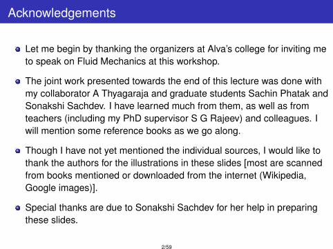
Let me begin by thanking the organizers at Alva’s college for inviting meto speak on Fluid Mechanics at this workshop.

The joint work presented towards the end of this lecture was done withmy collaborator A Thyagaraja and graduate students Sachin Phatak andSonakshi Sachdev. I have learned much from them, as well as fromteachers (including my PhD supervisor S G Rajeev) and colleagues. Iwill mention some reference books as we go along.

Though I have not yet mentioned the individual sources, I would like tothank the authors for the illustrations in these slides [most are scannedfrom books mentioned or downloaded from the internet (Wikipedia,Google images)].

Special thanks are due to Sonakshi Sachdev for her help in preparingthese slides.

2/59

Continuum, Fluid element, Local thermal equilibrium

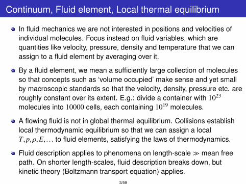
In fluid mechanics we are not interested in positions and velocities ofindividual molecules. Focus instead on fluid variables, which arequantities like velocity, pressure, density and temperature that we canassign to a fluid element by averaging over it.

By a fluid element, we mean a sufficiently large collection of moleculesso that concepts such as ‘volume occupied’ make sense and yet smallby macroscopic standards so that the velocity, density, pressure etc. areroughly constant over its extent. E.g.: divide a container with 1023

molecules into 10000 cells, each containing 1019 molecules.

A flowing fluid is not in global thermal equilibrium. Collisions establishlocal thermodynamic equilibrium so that we can assign a localT ,p,ρ,E, . . . to fluid elements, satisfying the laws of thermodynamics.

Fluid description applies to phenomena on length-scale mean freepath. On shorter length-scales, fluid description breaks down, butkinetic theory (Boltzmann transport equation) applies.

3/59

Eulerian and Lagrangian viewpoints

In the Eulerian description, we are interested in the time development offluid variables at a given point of observation ~r = (x,y,z). Interesting ifwe want to know how density changes, say, above my head. However,different fluid particles will arrive at the point ~r as time elapses.

It is also of interest to know how the corresponding fluid variablesevolve, not at a fixed location but for a fixed fluid element, as in aLagrangian description.

This is especially important since Newton’s second law applies directlyto fluid particles, not to point of observation!

So we ask how a variable changes along the flow, so that the observeris always attached to a fixed fluid element.

4/59

Leonhard Euler and Joseph Louis Lagrange

Figure: Leonhard Euler (left) and Joseph Louis Lagrange (right).

5/59

Material derivative measures rate of change along flow

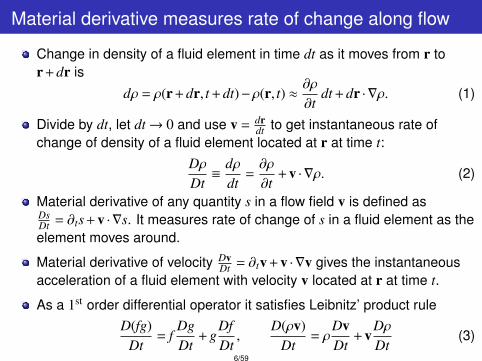
Change in density of a fluid element in time dt as it moves from r tor + dr is

dρ = ρ(r + dr, t + dt)−ρ(r, t) ≈∂ρ

∂tdt + dr · ∇ρ. (1)

Divide by dt, let dt→ 0 and use v = drdt to get instantaneous rate of

change of density of a fluid element located at r at time t:DρDt≡

dρdt

=∂ρ

∂t+ v · ∇ρ. (2)

Material derivative of any quantity s in a flow field v is defined asDsDt = ∂ts + v · ∇s. It measures rate of change of s in a fluid element as theelement moves around.

Material derivative of velocity DvDt = ∂tv + v · ∇v gives the instantaneous

acceleration of a fluid element with velocity v located at r at time t.

As a 1st order differential operator it satisfies Leibnitz’ product ruleD(fg)

Dt= f

DgDt

+ gDfDt,

D(ρv)Dt

= ρDvDt

+ vDρDt

(3)6/59

Continuity equation and incompressibility

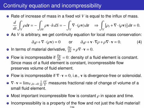
Rate of increase of mass in a fixed vol V is equal to the influx of mass.ddt

∫Vρdr = −

∫∂Vρv · n dS = −

∫V∇ · (ρv)dr ⇒

∫V

[ρt +∇ · (ρv)

]dr = 0.

As V is arbitrary, we get continuity equation for local mass conservation:

∂tρ+∇ · (ρv) = 0 or ∂tρ+ v · ∇ρ+ρ∇ ·v = 0. (4)

In terms of material derivative, DρDt +ρ∇ ·v = 0.

Flow is incompressible if DρDt = 0: density of a fluid element is constant.

Since mass of a fluid element is constant, incompressible flowpreserves volume of fluid element.

Flow is incompressible if ∇·v = 0, i.e., v is divergence-free or solenoidal.

∇ ·v = limV ,δt→01δtδVV measures fractional rate of change of volume of a

small fluid element.

Most important incompressible flow is constant ρ in space and time.

Incompressibility is a property of the flow and not just the fluid material!7/59

Sound speed, Mach number

Flow may be approximated as incompressible in regions where flow

speed is small compared to local sound speed cs =

√∂p∂ρ ∼

√γp/ρ for

adiabatic flow of an ideal gas with γ = Cp/Cv.

Recall that compressibility β =∂ρ∂p measures how much density can be

increased by increasing pressure. Incompressible fluid has β = 0, soc2 = 1/β =∞. In practice, an approximately incompressible fluid is onewith very large sound speed (much more than flow speeds).

Common flows in water are incompressible. So study of incompressibleflow is called hydrodynamics.

High speed flows in air/gases tend to be compressible. So compressibleflow is called aerodynamics or gas dynamics.

Incompressible hydrodynamics may be derived from compressible gasdynamic equations in the limit of small Mach number M = |v|/cs 1.

At high Mach numbers M 1 we have super-sonic flow andphenomena like shocks.

8/59

Newton’s 2nd law for fluid element: Inviscid Euler equation

Consider a fluid element of volume δV. Mass × acceleration is ρ(δV) DvDt .

Force on fluid element includes ‘body force’ like gravity derived from apotential φ. E.g. F = −ρ(δV)∇φ where −∇φ is acceleration due to gravity.

Also have surface force on a volume element, due to pressure exertedon it by neighbouring elements

Fsurface = −

∫∂V

p n dS = −

∫V∇pdV; if V = δV then Fsurf ≈ −∇p(δV).

Newton’s 2nd law then gives the celebrated (inviscid) Euler equation∂v∂t

+ v · ∇v = −∇pρ−∇φ; v · ∇v→ ‘advection term’ (5)

Continuity & Euler eqns. are first order in time derivatives: to solve initialvalue problem, must specify ρ(r, t = 0) and v(r, t = 0).

Boundary conditions: Euler equation is 1st order in space derivatives;impose BC on v, not ∂iv. On solid boundaries normal component ofvelocity vanishes v · n = 0. As |r| → ∞, typically v→ 0 and ρ→ ρ0.

9/59

Isaac Newton

Figure: Isaac Newton

10/59

Barotropic flow and specific enthalpy

Euler & continuity are 4 eqns for 5 unknowns ρ,v,p. Need another eqn.

In local thermodynamic equilibrium, pressure may be expressed as afunction of density and entropy. For isentropic flow it reduces to abarotropic relation p = p(ρ). It eliminates p and closes the system ofequations. E.g. p ∝ ργ adiabatic flow of ideal gas; p ∝ ρ for isothermal.

In barotropic flow, ∇p/ρ can be written as the gradient of an ‘enthalpy’

h(ρ) =

∫ ρ

ρ0

p′(ρ)ρ

dρ ⇒ ∇h = h′(ρ)∇ρ =p′(ρ)ρ∇ρ =

∇pρ. (6)

Reason for the name enthalpy: 1st law of thermodynamicsdU = TdS−pdV becomes dH = TdS + Vdp for enthalpy H = U + pV. Foran isentropic process dS = 0, so dH = Vdp.

Dividing by mass of fluid M we get d(H/M) = (V/M)dp. Definingenthalpy per unit mass h = H/M and density ρ = M/V gives dh = dp/ρ.

11/59

Barotropic flow and conserved energy

In barotropic flow p = p(ρ) and ∇p/ρ is gradient of enthalpy ∇h. So theEuler equation becomes

∂tv + v · ∇v = −∇h. (7)

Using the vector identity v · ∇v = ∇( 12 v2) + (∇×v)×v, we get

∂tv + (∇×v)×v = −∇

(h +

12

v2)

where ∇h =1ρ∇p. (8)

Barotropic flow has a conserved energy: kinetic + compressional

E =

∫ [12ρv2 + U(ρ)

]d3r, where U′(ρ) = h(ρ). (9)

U = p/(γ−1) for adiabatic flow of ideal gas. For monatomic ideal gasγ = 5/3 and compressional energy is (3/2)pV = (3/2)NkT.

More generally, the Euler and continuity equations are supplemented byan equation of state and energy equation (1st law of thermodynamics).

12/59

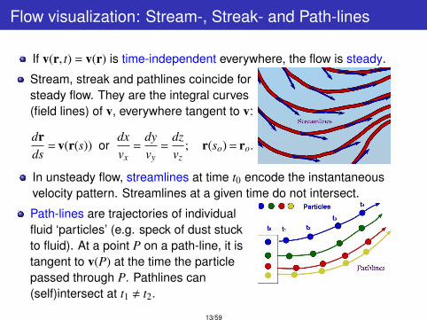
Flow visualization: Stream-, Streak- and Path-lines

If v(r, t) = v(r) is time-independent everywhere, the flow is steady.

Stream, streak and pathlines coincide forsteady flow. They are the integral curves(field lines) of v, everywhere tangent to v:

drds

= v(r(s)) ordxvx

=dyvy

=dzvz

; r(so) = ro.

In unsteady flow, streamlines at time t0 encode the instantaneousvelocity pattern. Streamlines at a given time do not intersect.

Path-lines are trajectories of individualfluid ‘particles’ (e.g. speck of dust stuckto fluid). At a point P on a path-line, it istangent to v(P) at the time the particlepassed through P. Pathlines can(self)intersect at t1 , t2.

13/59

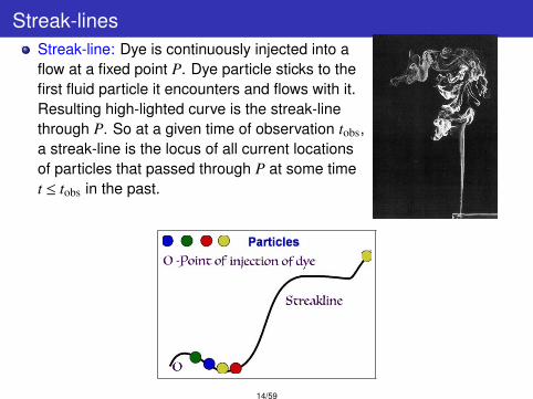
Streak-linesStreak-line: Dye is continuously injected into aflow at a fixed point P. Dye particle sticks to thefirst fluid particle it encounters and flows with it.Resulting high-lighted curve is the streak-linethrough P. So at a given time of observation tobs,a streak-line is the locus of all current locationsof particles that passed through P at some timet ≤ tobs in the past.

14/59

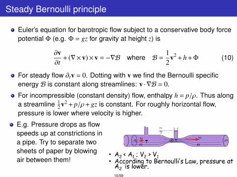
Steady Bernoulli principle

Euler’s equation for barotropic flow subject to a conservative body forcepotential Φ (e.g. Φ = gz for gravity at height z) is

∂v∂t

+ (∇×v)×v = −∇B where B =12

v2 + h +Φ (10)

For steady flow ∂tv = 0. Dotting with v we find the Bernoulli specificenergy B is constant along streamlines: v · ∇B = 0.

For incompressible (constant density) flow, enthalpy h = p/ρ. Thus alonga streamline 1

2 v2 + p/ρ+ gz is constant. For roughly horizontal flow,pressure is lower where velocity is higher.

E.g. Pressure drops as flowspeeds up at constrictions ina pipe. Try to separate twosheets of paper by blowingair between them!

15/59

Daniel Bernoulli

Figure: Daniel Bernoulli

16/59

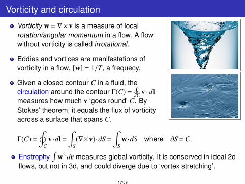
Vorticity and circulation

Vorticity w = ∇×v is a measure of localrotation/angular momentum in a flow. A flowwithout vorticity is called irrotational.

Eddies and vortices are manifestations ofvorticity in a flow. [w] = 1/T, a frequecy.

Given a closed contour C in a fluid, thecirculation around the contour Γ(C) =

∮C v ·dl

measures how much v ‘goes round’ C. ByStokes’ theorem, it equals the flux of vorticityacross a surface that spans C.

Γ(C) =

∮C

v ·dl =

∫S(∇×v) ·dS =

∫S

w ·dS where ∂S = C.

Enstrophy∫

w2 dr measures global vorticity. It is conserved in ideal 2dflows, but not in 3d, and could diverge due to ‘vortex stretching’.

17/59

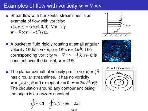
Examples of flow with vorticity w = ∇×vShear flow with horizontal streamlines is anexample of flow with vorticity:v(x,y,z) = (U(y),0,0). Vorticityw = ∇×v = −U′(y)z.

A bucket of fluid rigidly rotating at small angularvelocity Ωz has v(r, θ,z) = Ωz× r = Ωrθ. Thecorresponding vorticity w = ∇×v = 1

r ∂r(rvθ)z isconstant over the bucket, w = 2Ωz.

The planar azimuthal velocity profile v(r, θ) = cr θ

has circular streamlines. It has no vorticityw = 1

r ∂r(r cr )z = 0 except at r = 0: w = 2πcδ2(r)z.

The circulation around any contour enclosingthe origin is a nonzero constant∮

v ·dl =

∮(c/r)r dθ = 2πc

18/59

Freezing of w into v: Kelvin & Helmholtz theorems

Taking the curl of the Euler equation ∂tv + (∇×v)×v = −∇(h + 1

2 v2)

allows us to eliminate the pressure term in barotropic flow to get

∂tw +∇× (w×v) = 0. (11)

This may be interpreted as saying that vorticity is ‘frozen’ into v.

The flux of w through a surface moving with the flow is constant in time:ddt

∫St

w ·dS = 0 orddt

∮Ct

v ·dl =dΓ

dt= 0 where Ct = ∂St.

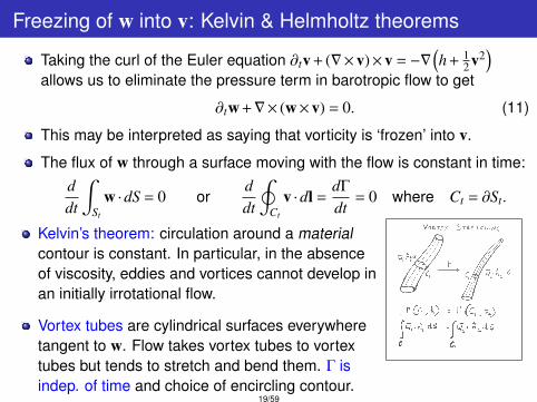
Kelvin’s theorem: circulation around a materialcontour is constant. In particular, in the absenceof viscosity, eddies and vortices cannot develop inan initially irrotational flow.

Vortex tubes are cylindrical surfaces everywheretangent to w. Flow takes vortex tubes to vortextubes but tends to stretch and bend them. Γ isindep. of time and choice of encircling contour.

19/59

Lord Kelvin and Hermann von Helmholtz

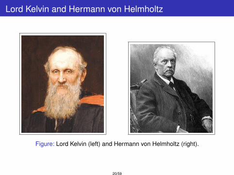
Figure: Lord Kelvin (left) and Hermann von Helmholtz (right).

20/59

Irrotational incompressible inviscid flow around cylinder

When flow is irrotational (w = ∇×v = 0) we may writev = −∇φ. Velocity potential φ is like the electrostaticpotential for ∇×E = 0.Incompressibility ∇ ·v = 0⇒ φ satisfies Laplace’s equation ∇2φ = 0.

We impose impenetrable boundary conditions: normal component ofvelocity vanishes on solid surfaces: ∂φ

∂n = 0 on boundary (Neumann BC).

Consider flow with asymptotic velocity −Ux past a fixed infinite cylinderof radius a with axis along z. Due to translation invariance along z, this isa 2d problem in the r, θ plane.

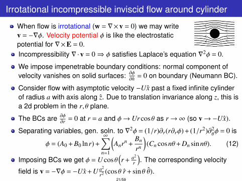
The BCs are ∂φ∂r = 0 at r = a and φ→ Ur cosθ as r→∞ (so v→−Ux).

Separating variables, gen. soln. to ∇2φ = (1/r)∂r(r∂rφ)+ (1/r2)∂2θφ = 0 is

φ = (A0 + B0 lnr) +

∞∑n=1

(Anrn +

Bn

rn

)(Cn cosnθ+ Dn sinnθ). (12)

Imposing BCs we get φ = U cosθ(r + a2

r

). The corresponding velocity

field is v = −∇φ = −Ux + U a2

r2 (cosθ r + sinθ θ).21/59

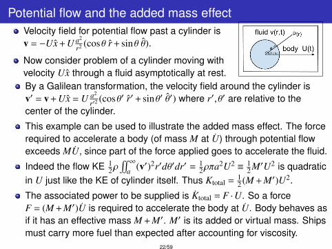
Potential flow and the added mass effectVelocity field for potential flow past a cylinder isv = −Ux + U a2

r2 (cosθ r + sinθ θ).

Now consider problem of a cylinder moving withvelocity Ux through a fluid asymptotically at rest.By a Galilean transformation, the velocity field around the cylinder isv′ = v + Ux = U a2

r′2 (cosθ′ r′+ sinθ′ θ′) where r′, θ′ are relative to thecenter of the cylinder.

This example can be used to illustrate the added mass effect. The forcerequired to accelerate a body (of mass M at U) through potential flowexceeds MU, since part of the force applied goes to accelerate the fluid.

Indeed the flow KE 12ρ! ∞

a (v′)2r′dθ′dr′ = 12ρπa2U2 ≡ 1

2 M′U2 is quadraticin U just like the KE of cylinder itself. Thus Ktotal = 1

2 (M + M′)U2.

The associated power to be supplied is Ktotal = F ·U. So a forceF = (M +M′)U is required to accelerate the body at U. Body behaves asif it has an effective mass M + M′. M′ is its added or virtual mass. Shipsmust carry more fuel than expected after accounting for viscosity.

22/59

Sound waves in compressible flow

Sound waves are excitations of the ρ or p fields. Arise in compressibleflows, where regions of compression and rarefaction can form.To derive the simplest equation for sound waves we linearize thecontinuity and Euler eqns around the static solution v = 0 and ρ = ρ0:

v = 0 + v1(r, t), ρ = ρ0 +ρ1(r, t) and p = p0 + p1(r, t). (13)

where v1,ρ1 and p1 are assumed small (treated to linear order).

Ignoring quadratic terms in small quantities, the continuity eqn.∂tρ+∇ · (ρv) = 0 becomes ∂tρ1 +ρ0∇ ·v1 = 0.

Assuming pressure variations are linear in density variations p1 = c2ρ1,the Euler eqn ρ(∂tv + v · ∇v) = −∇p becomes ρ0∂tv1 = −c2∇ρ1 or upontaking a divergence, ρ0∂t(∇ ·v1) = −c2∇2ρ1.

Eliminating ∇ ·v1 using continuity eqn we get the wave equation fordensity variations ∂2

t ρ1 = c2∇2ρ1. We identify c as the sound speed.

For incompressible flow, the sound speed is infinite: c2 =δpδρ →∞ as the

density variation is vanishingly small even for large pressure variations.23/59

Heat diffusion equation

Empirically it is found that the heat flux between bodies grows with thetemperature difference. Fourier’s law of heat diffusion states that theheat flux density vector (energy crossing unit area per unit time) isproportional to the negative gradient in temperature

q = −k∇T where k = thermal conductivity. (14)

Consider gas in a fixed volume V. The increase in internal energyU =

∫V ρcvTdr must be due to the influx of heat across its surface S.∫

V∂t(ρcvT)dr =

∫S

k∇T · n dS = k∫

V∇ ·∇T dr. (15)

cv = specific heat/mass (at constant volume, no work) and ρ = density.

V is arbitrary, so integrands must be equal. Heat equation follows:∂T∂t

= α∇2T where α =kρcv

is thermal diffusivity. (16)

Heat diffusion is dissipative, temperature differences even out and heatflow stops at equilibrium temperature. It is not time-reversible.

24/59

Including viscosity: Navier-Stokes equation

Heat equation ∂tT = α∇2T describes diffusion from hot→ cold regions.

(Shear) viscosity causes diffusion of velocity from a fast layer to aneighbouring slow layer of fluid. The viscous stress is ∝ velocitygradient. If a fluid is stirred and left, viscosity brings it to rest.

By analogy with heat diffusion, velocity diffusion is described by ν∇2v.

Kinematic viscosity ν has dimensions of diffusivity (areal velocity L2/T).

Postulate the Navier-Stokes equation for viscous incompressible flow:

vt + v · ∇v = −1ρ∇p + ν∇2v (NS). (17)

NS has not been derived from molecular dynamics except for dilutegases. It is the simplest equation consistent with physical requirementsand symmetries. It’s validity is restricted by experiment.

NS is second order in space derivatives unlike the inviscid Euler eqn.Experimentally relevant boundary condition is ‘no-slip’ at solid surfaces.

25/59

Claude Louis Navier, Saint Venant and George Stokes

Figure: Claude Louis Navier (left), Saint Venant (middle) and George Gabriel Stokes(right).

26/59

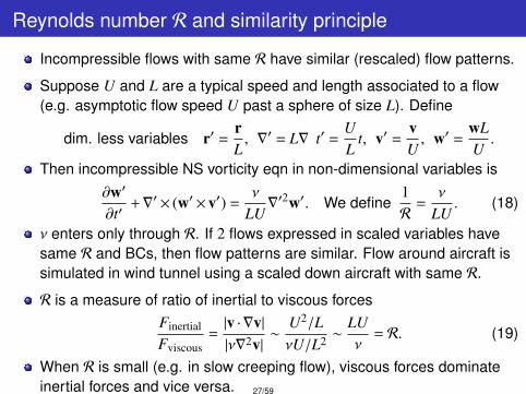
Reynolds number R and similarity principle

Incompressible flows with same R have similar (rescaled) flow patterns.

Suppose U and L are a typical speed and length associated to a flow(e.g. asymptotic flow speed U past a sphere of size L). Define

dim. less variables r′ =rL, ∇′ = L∇ t′ =

UL

t, v′ =vU, w′ =

wLU.

Then incompressible NS vorticity eqn in non-dimensional variables is∂w′

∂t′+∇′× (w′×v′) =

ν

LU∇′2w′. We define

1R

=ν

LU. (18)

ν enters only through R. If 2 flows expressed in scaled variables havesame R and BCs, then flow patterns are similar. Flow around aircraft issimulated in wind tunnel using a scaled down aircraft with same R.

R is a measure of ratio of inertial to viscous forcesFinertial

Fviscous=|v · ∇v||ν∇2v|

∼U2/LνU/L2 ∼

LUν

= R. (19)

When R is small (e.g. in slow creeping flow), viscous forces dominateinertial forces and vice versa. 27/59

Osbourne Reynolds

Figure: Osbourne Reynolds

28/59

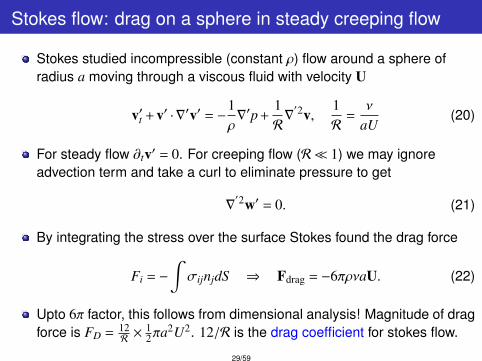
Stokes flow: drag on a sphere in steady creeping flow

Stokes studied incompressible (constant ρ) flow around a sphere ofradius a moving through a viscous fluid with velocity U

v′t + v′ · ∇′v′ = −1ρ∇′p +

1R∇′2v,

1R

=ν

aU(20)

For steady flow ∂tv′ = 0. For creeping flow (R 1) we may ignoreadvection term and take a curl to eliminate pressure to get

∇′2w′ = 0. (21)

By integrating the stress over the surface Stokes found the drag force

Fi = −

∫σijnjdS ⇒ Fdrag = −6πρνaU. (22)

Upto 6π factor, this follows from dimensional analysis! Magnitude of dragforce is FD = 12

R× 1

2πa2U2. 12/R is the drag coefficient for stokes flow.

29/59

Drag on a sphere at higher Reynolds number

At higher speeds (R 1), naively expect viscous term to be negligible.However, experimental flow is far from ideal (inviscid) flow!At higher R, flow becomes unsteady, vorticesdevelop downstream and eventually a turbulentwake is generated.

Dimensional analysis implies drag force on asphere is expressible as FD = 1

2 CD(R) πa2 ρU2,

where CD = CD(R) is the dimensionless dragcoefficient, determined by NS equation.

Comparing with Stokes’ formula for creepingflow at R 1 we must have CD ∼ 12/R asR→ 0.

Significant experimental deviations from Stokes’law: enhancement of drag at higher 1 ≤ R ≤ 105,then drag drops with increasing U!

30/59

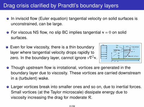
Drag crisis clarified by Prandtl’s boundary layers

In inviscid flow (Euler equation) tangential velocity on solid surfaces isunconstrained, can be large.

For viscous NS flow, no slip BC implies tangential v = 0 on solidsurfaces.

Even for low viscosity, there is a thin boundarylayer where tangential velocity drops rapidly tozero. In the boundary layer, cannot ignore ν∇2v.

Though upstream flow is irrotational, vortices are generated in theboundary layer due to viscosity. These vortices are carried downstreamin a (turbulent) wake.

Larger vortices break into smaller ones and so on, due to inertial forces.Small vortices (at the Taylor microscale) dissipate energy due toviscosity increasing the drag for moderate R.

31/59

Ludwig Prandtl

Figure: Ludwig Prandtl

32/59

2D Incompressible flows: stream function

In 2D incompressible flow the velocity components are expressible asderivatives of a stream function: v = (u,v) = (−ψy,ψx). Incompressibilitycondition ∇ ·v = −ψyx +ψxy = 0 is identically satisfied.

Streamlines defined by dxu =

dyv are level

curves of ψ. For, along a streamlinedψ = (∂xψ)dx + (∂yψ)dy = vdx−udy = 0.

If in addition, flow is irrotational(w = ∇×v = 0), then v admits a velocitypotential v = −∇φ so that (u,v) = (−φx,−φy).

So φ & ψ satisfy the Cauchy Riemann equations: φx = ψy, φy = −ψx andthe complex velocity potential f = φ+ iψ is analytic! φ and ψ areharmonic. ∇2φ = 0⇒ incompressible and w = ∇2ψz = 0⇒ irrotational.

The level curves of ψ and φ are orthogonal : ∇φ ·∇ψ = −(u,v) · (v,−u) = 0.

Complex velocity u− iv is the derivative −f ′(z) of the complex potential.33/59

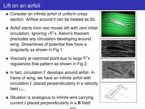
Lift on an airfoilConsider an infinite airfoil of uniform crosssection. Airflow around it can be treated as 2d.

Airfoil starts from rest moves left with zero initialcirculation. Ignoring ν∇2v, Kelvin’s theoremprecludes any circulation developing aroundwing. Streamlines of potential flow have asingularity as shown in Fig 1.

Viscosity at rearmost point due to large ∇2vregularizes flow pattern as shown in Fig 2.

In fact, circulation Γ develops around airfoil. Inframe of wing, we have an infinite airfoil withcirculation Γ placed perpendicularly in a velocityfield v∞.

Situation is analogous to infinite wire carryingcurrent I placed perpendicularly in a B field!

34/59

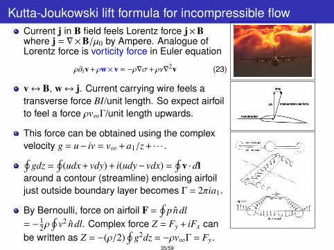
Kutta-Joukowski lift formula for incompressible flowCurrent j in B field feels Lorentz force j×Bwhere j = ∇×B/µ0 by Ampere. Analogue ofLorentz force is vorticity force in Euler equation

ρ∂tv +ρw×v = −ρ∇σ+ρν∇2v (23)

v↔ B, w↔ j. Current carrying wire feels atransverse force BI/unit length. So expect airfoilto feel a force ρv∞Γ/unit length upwards.

This force can be obtained using the complexvelocity g = u− iv = v∞+ a1/z + · · · .∮

gdz =∮

(udx + vdy) + i(udy− vdx) =∮

v ·dlaround a contour (streamline) enclosing airfoiljust outside boundary layer becomes Γ = 2πia1.

By Bernoulli, force on airfoil F =∮

pndl= − 1

2ρ∮

v2 ndl. Complex force Z = Fy + iFx canbe written as Z = −(ρ/2)

∮g2dz = −ρv∞Γ = Fy.

35/59

Nikolay Yegorovich Zhukovsky and Martin Wilhelm Kutta

Figure: Nikolay Yegorovich Zhukovsky (left) and Martin Wilhelm Kutta (right).

36/59

Transition from laminar to turbulent flow past a cylinder

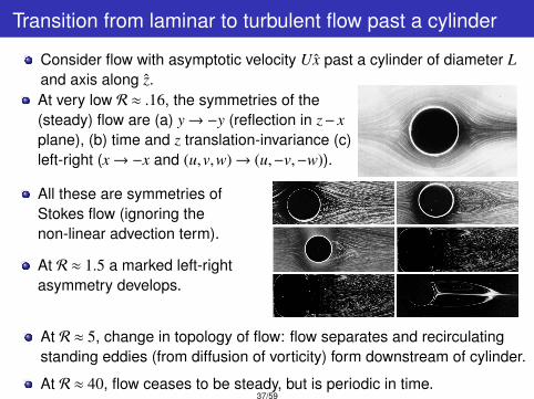
Consider flow with asymptotic velocity Ux past a cylinder of diameter Land axis along z.At very low R ≈ .16, the symmetries of the(steady) flow are (a) y→−y (reflection in z− xplane), (b) time and z translation-invariance (c)left-right (x→−x and (u,v,w)→ (u,−v,−w)).

All these are symmetries ofStokes flow (ignoring thenon-linear advection term).

At R ≈ 1.5 a marked left-rightasymmetry develops.

At R ≈ 5, change in topology of flow: flow separates and recirculatingstanding eddies (from diffusion of vorticity) form downstream of cylinder.

At R ≈ 40, flow ceases to be steady, but is periodic in time.37/59

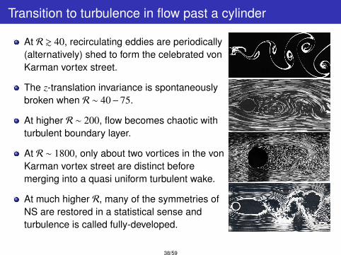
Transition to turbulence in flow past a cylinder

At R & 40, recirculating eddies are periodically(alternatively) shed to form the celebrated vonKarman vortex street.

The z-translation invariance is spontaneouslybroken when R ∼ 40−75.

At higher R ∼ 200, flow becomes chaotic withturbulent boundary layer.

At R ∼ 1800, only about two vortices in the vonKarman vortex street are distinct beforemerging into a quasi uniform turbulent wake.

At much higher R, many of the symmetries ofNS are restored in a statistical sense andturbulence is called fully-developed.

38/59

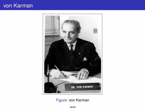
von Karman

Figure: von Karman

39/59

What is turbulence? Key features.

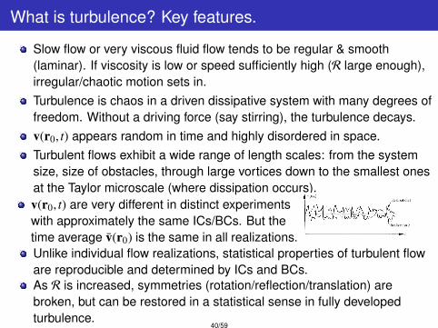
Slow flow or very viscous fluid flow tends to be regular & smooth(laminar). If viscosity is low or speed sufficiently high (R large enough),irregular/chaotic motion sets in.Turbulence is chaos in a driven dissipative system with many degrees offreedom. Without a driving force (say stirring), the turbulence decays.v(r0, t) appears random in time and highly disordered in space.Turbulent flows exhibit a wide range of length scales: from the systemsize, size of obstacles, through large vortices down to the smallest onesat the Taylor microscale (where dissipation occurs).v(r0, t) are very different in distinct experimentswith approximately the same ICs/BCs. But thetime average v(r0) is the same in all realizations.Unlike individual flow realizations, statistical properties of turbulent floware reproducible and determined by ICs and BCs.As R is increased, symmetries (rotation/reflection/translation) arebroken, but can be restored in a statistical sense in fully developedturbulence.

40/59

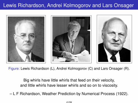
Lewis Richardson, Andrei Kolmogorov and Lars Onsager

Figure: Lewis Richardson (L), Andrei Kolmogorov (C) and Lars Onsager (R).

Big whirls have little whirls that feed on their velocity,and little whirls have lesser whirls and so on to viscosity.

– L F Richardson, Weather Prediction by Numerical Process (1922).

41/59

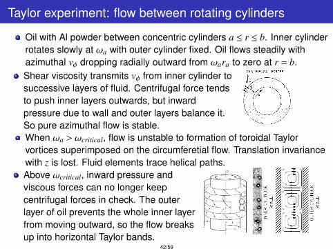
Taylor experiment: flow between rotating cylinders

Oil with Al powder between concentric cylinders a ≤ r ≤ b. Inner cylinderrotates slowly at ωa with outer cylinder fixed. Oil flows steadily withazimuthal vφ dropping radially outward from ωara to zero at r = b.Shear viscosity transmits vφ from inner cylinder tosuccessive layers of fluid. Centrifugal force tendsto push inner layers outwards, but inwardpressure due to wall and outer layers balance it.So pure azimuthal flow is stable.When ωa > ωcritical, flow is unstable to formation of toroidal Taylorvortices superimposed on the circumferetial flow. Translation invariancewith z is lost. Fluid elements trace helical paths.Above ωcritical, inward pressure andviscous forces can no longer keepcentrifugal forces in check. The outerlayer of oil prevents the whole inner layerfrom moving outward, so the flow breaksup into horizontal Taylor bands.

42/59

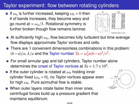
Taylor experiment: flow between rotating cylindersIf ωa is further increased, keeping ωb = 0 then# of bands increases, they become wavy andgo round at ≈ ωa/3. Rotational symmetry isfurther broken though flow remains laminar.

At sufficiently high ωa, flow becomes fully turbulent but time averageflow displays approximate Taylor vortices and cells.There are 3 convenient dimensionless combinations in this problem:(b−a)/a, L/a and the Taylor number Ta = ω2

aa(b−a)3/ν2.

For small annular gap and tall cylinders, Taylor number alonedetermines the onset of Taylor vortices at Ta = 1.7×104.If the outer cylinder is rotated at ωb holding innercylinder fixed (ωa = 0), no Taylor vortices appear evenfor high ωb. Pure azimuthal flow is stable.When outer layers rotate faster than inner ones,centrifugal forces build up a pressure gradient thatmaintains equilibrium.

43/59

Geoffrey Ingram Taylor

Figure: Geoffrey Ingram Taylor

44/59

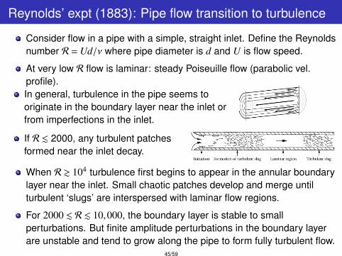
Reynolds’ expt (1883): Pipe flow transition to turbulence

Consider flow in a pipe with a simple, straight inlet. Define the Reynoldsnumber R = Ud/ν where pipe diameter is d and U is flow speed.

At very low R flow is laminar: steady Poiseuille flow (parabolic vel.profile).In general, turbulence in the pipe seems tooriginate in the boundary layer near the inlet orfrom imperfections in the inlet.

If R . 2000, any turbulent patchesformed near the inlet decay.

When R & 104 turbulence first begins to appear in the annular boundarylayer near the inlet. Small chaotic patches develop and merge untilturbulent ‘slugs’ are interspersed with laminar flow regions.

For 2000 . R . 10,000, the boundary layer is stable to smallperturbations. But finite amplitude perturbations in the boundary layerare unstable and tend to grow along the pipe to form fully turbulent flow.

45/59

Shocks in compressible flow

A shock is usually a surface of small thickness across which v,p,ρchange significantly: modelled as a surface of discontinuity.

Shock moves faster than the speed of sound. Roughly, if shockpropagates sub-sonically, it could emit sound waves ahead of the shockthat eliminate the discontinuity. Mach number M = v1/c > 1.

Sudden localized explosions like supernovae or bombs often producespherical shocks called blast waves. Nature of spherical blast wave fromatom bomb was worked out by Sedov and Taylor in the 1940s.

Material from undisturbed medium in front of shock (ρ1) moves behindthe shock and gets compressed to ρ2.

Fluxes of mass, momentum and energy are equal in front of and behindthe shock. This may be used to relate ρ1,v1,p1 to ρ2,v2,p2. These leadto the Rankine-Hugoniot ‘jump’ conditions.

Viscous term ν∇2v is often important in a shock since v changes rapidly.Leads to heating of the gas and entropy production.

46/59

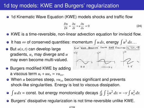
1d toy models: KWE and Burgers’ regularization

1d Kinematic Wave Equation (KWE) models shocks and traffic flow

DuDt

=∂u∂t

+ u∂u∂x

= 0 (24)

KWE is a time-reversible, non-linear advection equation for inviscid flow.

It has ∞ of conserved quantities: momentum∫

u dx, energy∫

u2 dx . . .

But u(x, t) can develop largegradients, ux may diverge and umay even become multi-valued.

Burgers modified KWE by addinga viscous term ut + uux = νuxx.When u becomes steep, νuxx becomes significant and preventsshock-like singularities. Energy is lost to viscous dissipation.∫

u dx = const. but energy monotonically decays ddt

∫12 u2 dx = −ν

∫u2

x dx

Burgers’ dissipative regularization is not time-reversible unlike KWE.47/59

Conservative regularization of KWE: KdV equation

KdV models nonlinear non-dissipative dispersive water waves

ut −6uux + uxxx, u = height of wave. (25)

KdV admits infinitely many conservation laws, a Hamiltonian andPoisson bracket formulation and is exactly solvable via IST.

u = u,H, H =

∫ [12

u2x + u3

]dx, u(x),u(y) =

12

(∂x−∂y)δ(x− y). (26)

It also has a discrete ‘time-reversal’ (PT) symmetryt→−t,x→−x,u→ u.

The 3rd order dispersive term prevents development of large gradientsof u. Smooth solutions exist for arbitrarily long times. Displays recurrentmotions in bounded domains.

KdV has cnoidal (periodic) and finitely many interacting, exact N-solitonsolutions: competing effects of non-linear advection and dispersionresult in soliton preserving its shape under time evolution.

48/59

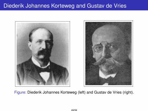
Diederik Johannes Korteweg and Gustav de Vries

Figure: Diederik Johannes Korteweg (left) and Gustav de Vries (right).

49/59

Conservative regularization of compressible 3d Euler

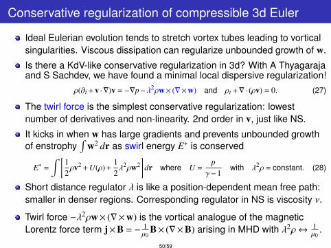
Ideal Eulerian evolution tends to stretch vortex tubes leading to vorticalsingularities. Viscous dissipation can regularize unbounded growth of w.

Is there a KdV-like conservative regularization in 3d? With A Thyagarajaand S Sachdev, we have found a minimal local dispersive regularization!

ρ(∂t + v · ∇)v = −∇p−λ2ρw× (∇×w) and ρt +∇ · (ρv) = 0. (27)

The twirl force is the simplest conservative regularization: lowestnumber of derivatives and non-linearity. 2nd order in v, just like NS.

It kicks in when w has large gradients and prevents unbounded growthof enstrophy

∫w2 dr as swirl energy E∗ is conserved

E∗ =

∫ [12ρv2 + U(ρ) +

12λ2ρw2

]dr where U =

pγ−1

with λ2ρ = constant. (28)

Short distance regulator λ is like a position-dependent mean free path:smaller in denser regions. Corresponding regulator in NS is viscosity ν.

Twirl force −λ2ρw× (∇×w) is the vortical analogue of the magneticLorentz force term j×B = − 1

µ0B× (∇×B) arising in MHD with λ2ρ↔ 1

µ0.

50/59

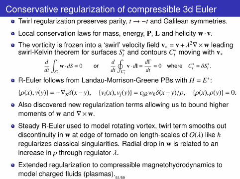
Conservative regularization of compressible 3d EulerTwirl regularization preserves parity, t→−t and Galilean symmetries.

Local conservation laws for mass, energy, P, L and helicity w ·v.

The vorticity is frozen into a ‘swirl’ velocity field v∗ = v +λ2∇×w leadingswirl-Kelvin theorem for surfaces S∗t and contours C∗t moving with v∗

ddt

∫S∗t

w ·dS = 0 orddt

∮C∗t

v ·dl =dΓ

dt= 0 where C∗t = ∂S∗t .

R-Euler follows from Landau-Morrison-Greene PBs with H = E∗:

ρ(x),v(y) = −∇xδ(x−y), vi(x),vj(y) = εijkwkδ(x−y)/ρ, ρ(x),ρ(y) = 0.

Also discovered new regularization terms allowing us to bound highermoments of w and ∇×w.

Steady R-Euler used to model rotating vortex, twirl term smooths outdiscontinuity in w at edge of tornado on length-scales of O(λ) like hregularizes classical singularities. Radial drop in w is related to anincrease in ρ through regulator λ.

Extended regularization to compressible magnetohydrodynamics tomodel charged fluids (plasmas).

51/59

Added-mass Higgs mechanism analogy

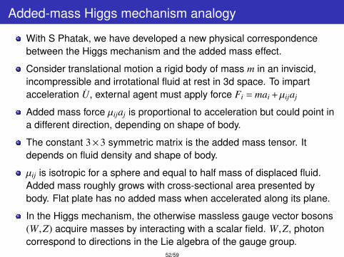
With S Phatak, we have developed a new physical correspondencebetween the Higgs mechanism and the added mass effect.

Consider translational motion a rigid body of mass m in an inviscid,incompressible and irrotational fluid at rest in 3d space. To impartacceleration U, external agent must apply force Fi = mai +µijaj

Added mass force µijaj is proportional to acceleration but could point ina different direction, depending on shape of body.

The constant 3×3 symmetric matrix is the added mass tensor. Itdepends on fluid density and shape of body.

µij is isotropic for a sphere and equal to half mass of displaced fluid.Added mass roughly grows with cross-sectional area presented bybody. Flat plate has no added mass when accelerated along its plane.

In the Higgs mechanism, the otherwise massless gauge vector bosons(W,Z) acquire masses by interacting with a scalar field. W,Z, photoncorrespond to directions in the Lie algebra of the gauge group.

52/59

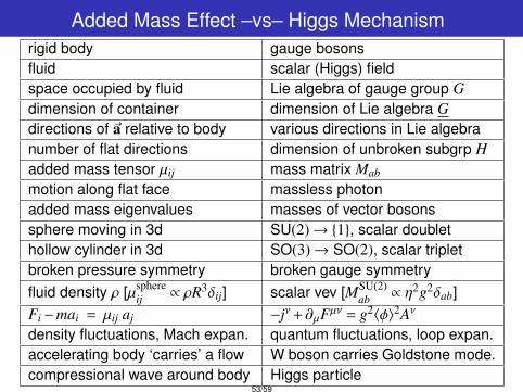
Added Mass Effect –vs– Higgs Mechanismrigid body gauge bosonsfluid scalar (Higgs) fieldspace occupied by fluid Lie algebra of gauge group Gdimension of container dimension of Lie algebra Gdirections of ~a relative to body various directions in Lie algebranumber of flat directions dimension of unbroken subgrp Hadded mass tensor µij mass matrix Mab

motion along flat face massless photonadded mass eigenvalues masses of vector bosonssphere moving in 3d SU(2)→ 1, scalar doublethollow cylinder in 3d SO(3)→ SO(2), scalar tripletbroken pressure symmetry broken gauge symmetryfluid density ρ [µsphere

ij ∝ ρR3δij] scalar vev [MSU(2)ab ∝ η2g2δab]

Fi−mai = µij aj −jν +∂µFµν = g2〈φ〉2Aν

density fluctuations, Mach expan. quantum fluctuations, loop expan.accelerating body ‘carries’ a flow W boson carries Goldstone mode.compressional wave around body Higgs particle

53/59

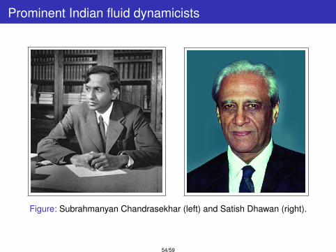
Prominent Indian fluid dynamicists

Figure: Subrahmanyan Chandrasekhar (left) and Satish Dhawan (right).

54/59

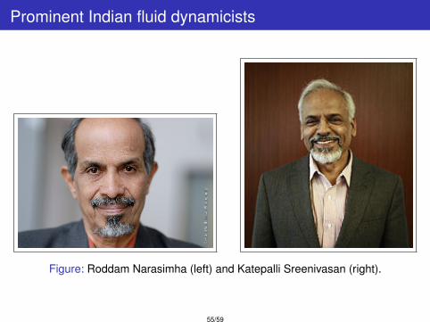
Prominent Indian fluid dynamicists

Figure: Roddam Narasimha (left) and Katepalli Sreenivasan (right).

55/59

Existence & Regularity: Clay Millenium Problem

Either prove the existence and regularity of solutions to incompressibleNS subject to smooth initial data [in R3 or in a cube with periodic BCs]OR show that a smooth solution could cease to exist after a finite time.

J Leray (1934) proved that weak solutions to NS exist, but need not beunique and could not rule out singularities.

Hausdorff dim of set of space-time points where singularities can occurin NS cannot exceed one. So hypothetical singularities are rare!

O Ladyzhenskaya (1969) showed existence and regularity of classicalsolutions to NS regularized with hyperviscosity −µ(−∇2)αv with α ≥ 2.J-L Lions (1969) extended it to α ≥ 5/4.

A proof of existence/uniqueness/smoothness of solutions to NS or ademonstration of finite time blow-up is mathematically important.

Physically, it is know that for large enough R, most laminar flows areunstable, they become turbulent and seem irregular. Methods tocalculate/predict features of turbulent flows would also be very valuable.

56/59

Jean Leray, Olga Ladyzhenskaya and Jacques LouisLions

Figure: Jean Leray (left), Olga Ladyzhenskaya (middle) and Jacques Louis Lions(right).

57/59

References

Choudhuri A R , The physics of Fluids and Plasmas: An introduction for astrophysicists, Camb.Univ Press, Cambridge (1998).

Davidson P A, Turbulence: An introduction for scientists and engineers , Oxford Univ Press, NewYork (2004).

Feynman R, Leighton R and Sands M, The Feynman lectures on Physics: Vol 2, Addison-WesleyPublishing (1964). Reprinted by Narosa Publishing House (1986).

Frisch U, Turbulence The Legacy of A. N. Kolmogorov Camb. Univ. Press (1995).

Landau L D and Lifshitz E M , Fluid Mechanics, 2nd Ed. Pergamon Press (1987).

Van Dyke M, An album of fluid motion, The Parabolic Press, Stanford, California (1988).

Thyagaraja A, Conservative regularization of ideal hydrodynamics and magnetohydrodynamics,Physics of Plasmas 17 , 032503 (2010).

Krishnaswami G S, Sachdev S and Thyagaraja A, Conservative regularization of compressible flow,arXiv:1510.01606 (2015).

Krishnaswami G S, Sachdev S and Thyagaraja A, Local conservative regularizations ofcompressible magnetohydrodynamic and neutral flows, arXiv:1602.04323, Phys. Plasmas 23,022308 (2016).

Krishnaswami G S and Phatak S S, Higgs Mechanism and the Added-Mass Effect, Proc. R. Soc. A471: 20140803, (2015).

58/59

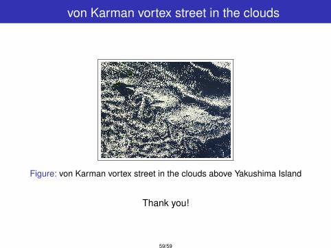
von Karman vortex street in the clouds

Figure: von Karman vortex street in the clouds above Yakushima Island

Thank you!

59/59