Goodwin, Graebe, Salgado ©, Prentice Hall 2000 Chapter 16 Control Design Based on Optimization.

Goodwin, Graebe, Salgado ©, Prentice Hall 2000Chapter 16

Chapter 16

Control Design Based on Control Design Based on OptimizationOptimization


Thus far, we have seen that design constraints arise from a number of different sources: structural plant properties, such as NMP zeros or unstable

poles;

disturbances - their frequency content, point of injection, and measurability;

architectural properties and the resulting algebraic laws of trade-off; and

integral constraints and the resulting integral laws of trade-off.


The subtlety as well as complexity of the emergent trade-off web, into which the designer needs to ease a solution, motivates interest in what is known as criterion-based control design or optimal control theory “the aim here is to capture the control objective in a mathematical criterion and solve it for the controller that (depending on the formulation) maximizes or minimizes it”.


Three questions arise:

1. Is optimization of the criterion mathematically feasible?

2. How good is the resulting controller?

3. Can the constraint of the trade-off web be circumvented by optimization?


Optimal Q Synthesis

In this chapter, we will combine the idea of Q synthesis with a quadratic optimization strategy to formulate the design problem.

This approach is facilitated by the fact, already observed, that the nominal sensitivity functions are affine functions of Q(s).


Assume that a target function H0(s) is chosen for the complementary sensitivity T0(s). We have seen in Chapter 15 that, if we are given some stabilizing controller C(s) = P(s)/L(s), then all stabilizing controllers can be expressed as

the nominal complementary sensitivity function is then given by


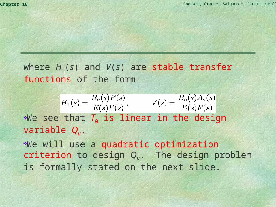
where H1(s) and V(s) are stable transfer functions of the form

We see that T0 is linear in the design variable Qu.

We will use a quadratic optimization criterion to design Qu. The design problem is formally stated on the next slide.


Quadratic Optimal Synthesis

Let S denote the set of all real rational stable transfer functions; then the quadratic optimal synthesis problem can be stated as follows:

Problem (Quadratic optimal synthesis problem). Find such that S)(0 sQu


The criterion on the previous slide uses the quadratic norm, also called the H2-norm, of a function X(s) defined as (continuous-time)

and in discrete time2/1

2

0

22/1

2

02)(

21

)()(21

)(

deXdeXeXzX jjj

2/12

2/1

2)(

21

)()(21

)(

djXdjXjXsX


To solve this problem, we first need a preliminary result that is an extension of Pythagoras’ theorem.

Lemma 16.1: Let S0 S be the set of all real strictly proper stable rational functions, and let be the set of all real strictly proper rational functions that are analytical for {s}0. Furthermore assume that Xs(s) S0 and Xu(s) . Then

Proof: See the book.

0S

0S


To use the above result, we will need to split a general function X(s) into a stable part Xs(s) and an unstable part Xu(s).

We can do this via a partial-fraction expansion. The stable poles and their residues constitute the stable part.


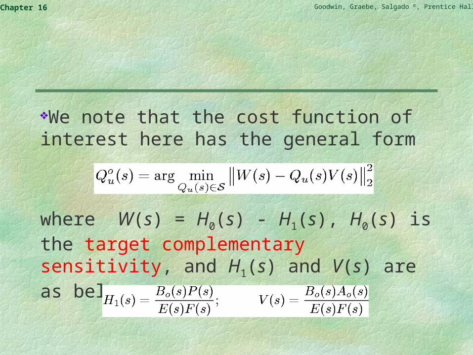
We note that the cost function of interest here has the general form

where W(s) = H0(s) - H1(s), H0(s) is the target complementary sensitivity, and H1(s) and V(s) are as below:


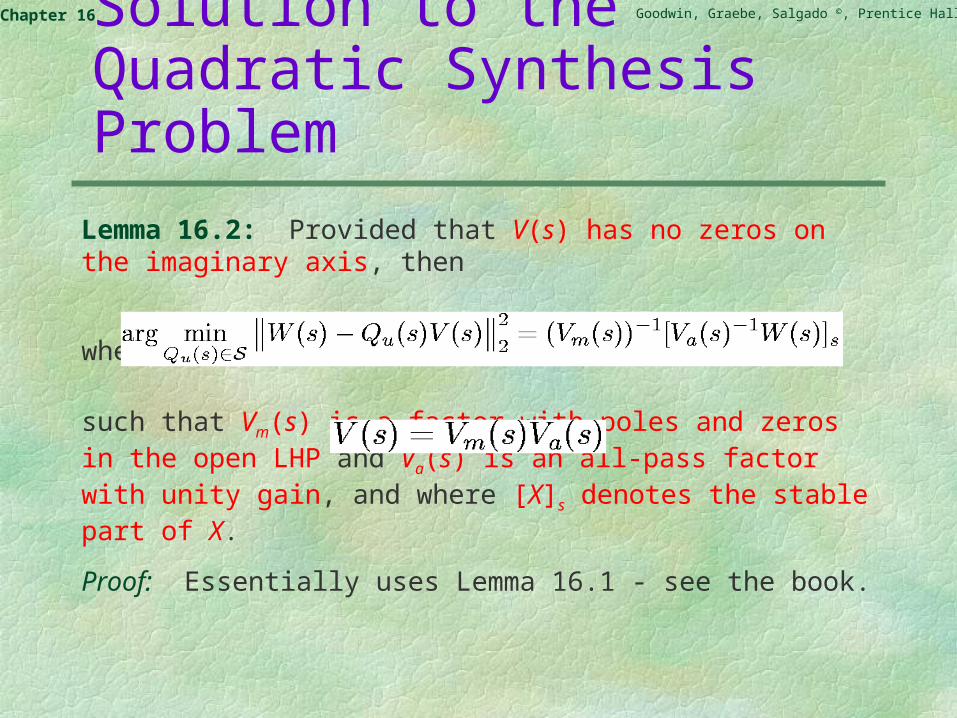
Solution to the Quadratic Synthesis Problem

Lemma 16.2: Provided that V(s) has no zeros on the imaginary axis, then

where

such that Vm(s) is a factor with poles and zeros in the open LHP and Va(s) is an all-pass factor with unity gain, and where [X]s denotes the stable part of X.

Proof: Essentially uses Lemma 16.1 - see the book.


The solution will be proper only either if V has relative degree zero or if both V has relative degree one and W has relative degree of at least one. However, improper solutions can readily be turned into approximate proper solutions by adding an appropriate number of fast poles to ).(0 sQu


Returning to the problem posed earlier, we see that Lemma 16.2 provided an immediate solution, by setting

=

To(s)


The above procedure can be modified to include a weighting function (j) “In order to stress the range of frequencies of interest”. In this framework, the cost function is now given by

No additional difficulty arises, because it is enough to simply redefine V(s) and W(s) to convert the problem into the form


It is also possible to restrict the solution space to satisfy additional design specifications. For example, forcing an integration is achieved by parameterizing Q(s) as and introducing a weighting function (s) = 1/s. (H0(0) = 1 is also required). This does not alter the affine nature of T0(s) on the unknown function. Hence, the synthesis procedure developed above can be applied, provided that we first redefine the function, V(s) and W(s).


Example 16.1: Unstable Plant

Consider a plant with nominal model

Assume that the target function for T0(s) is given by


We first choose the observer polynomial E(s) = (s+4)(s+10) and the controller polynomial F(s) = s2 + 4s + 9=(s+2)2+5 “the roots of E(s) are selected with faster dynamics than F(s)” . We then solve the pole-assignment equation A0(s)L(s) + B0(s)P(s) = E(s)F(s) to obtain the prestabilizing control law expressed in terms of P(s) and L(s). The resultant polynomials are


Now consider any controller from the class of stabilizing control laws as parameterized in

The quadratic cost function is then as in


Consequently

The optimal Qu(s) is then obtained


We observe that is improper. However, we can approximate it by a suboptimal (but proper) transfer function, by adding one fast pole to

:

)(0 sQu

),(~ sQ

)(0 sQu


Example 16.2: Nonminimum-phase Plant

Consider a plant with nominal model

It is required to synthesize, by using H2 optimization, a one-d.o.f. control loop having the target function

and to provide exact model inversion at = 0 (integral action).


The appropriate cost function is defined as (stable factorization To(s)=Q(s)Go(s))

Then the cost function takes the form

where

18


We first note that

The optimal can then be obtained by using

from this Q0(s) can be obtained as One fast pole has to be added to make this function proper.

)( sQ

.1)()( 00 sQssQ


Robust Control Design with Confidence Bounds

We next show briefly how optimization methods can be used to change a nominal controller so that the resultant performance is robust against model errors.

For the sake of argument we will use statistical confidence bounds - although other types of modelling error can also be used.


Statistical Confidence Bounds

We have argued in Chapter 3 that no model can give an exact description of a real process.

Our starting point will be to assume the existence of statistical confidence bounds on the modeling error.

In particular, we assume that we are given a nominal frequency response, G0(j), together with a statistical description of the associated errors of the form

where G(j) is the true (but unknown) frequency response and G(j), as usual, represents the additive modeling error.


We assume that G possesses the following probabilistic properties:

(s) is the stable, minimum-phase spectral factor. Also, is the given measure of the modeling error.

The function would normally be obtained from some kind of identification procedure.

~


Robust Control Design

Based on the nominal model G0(j), we assume that a design is carried out that leads to acceptable nominal performance. This design will typically account for the usual control-design issues such as nonminimum-phase behavior, the available input range, and unstable poles. Let us say that this has been achieved with a nominal controller C0 and that the corresponding nominal sensitivity function is S0. Of course, the value S0 will not be achieved in practice, because of the variability of the achieved sensitivity, S, from S0.


Let us assume, to begin, that the open-loop system is stable. We can thus use the simple form of the parameterization of all stabilizing controllers to express C0 and S0 in terms of a stable parameter Q0.


The achieved sensitivity, S1, when the nominal controller C0 is applied to the true plant is given by

where G is the additive model error.


Our proposal for robust design now is to adjust the controller so that the distance between the resulting achieved sensitivity, S1, and S0 is minimized. If we change Q0 to Q and hence C0 to C, then the achieved sensitivity changes to


Where

and

Observe that S1 denotes, the sensitivity achieved when the plant is G0 and the controller is parameterized by Q, and S0 denotes the sensitivity achieved when the plant is G0 and the controller is parameterized by Q0.


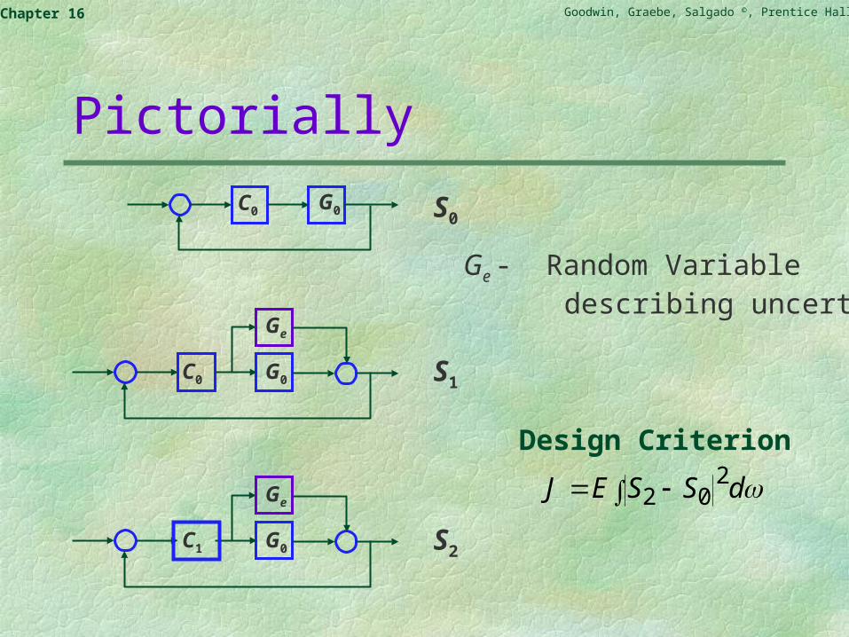
Pictorially

Ge - Random Variable describing uncertainty

dSSEJ 202

Design Criterion

S0

S1

S2

C0 G0

C0 G0

Ge

C1 G0

Ge


Frequency Weighted Errors

Unfortunately, (S2 - S0) is a nonlinear function of Q and G.

In place of minimizing some measure of the sensitivity error, we instead consider a weighted version with W2 = 1+GQ. Thus, consider

where is the desired adjustment in Q0(s) to account for G(s).

)()()(~0 sQsQsQ


The procedure that we now propose for choosing is to find the value that minimizes

Q~


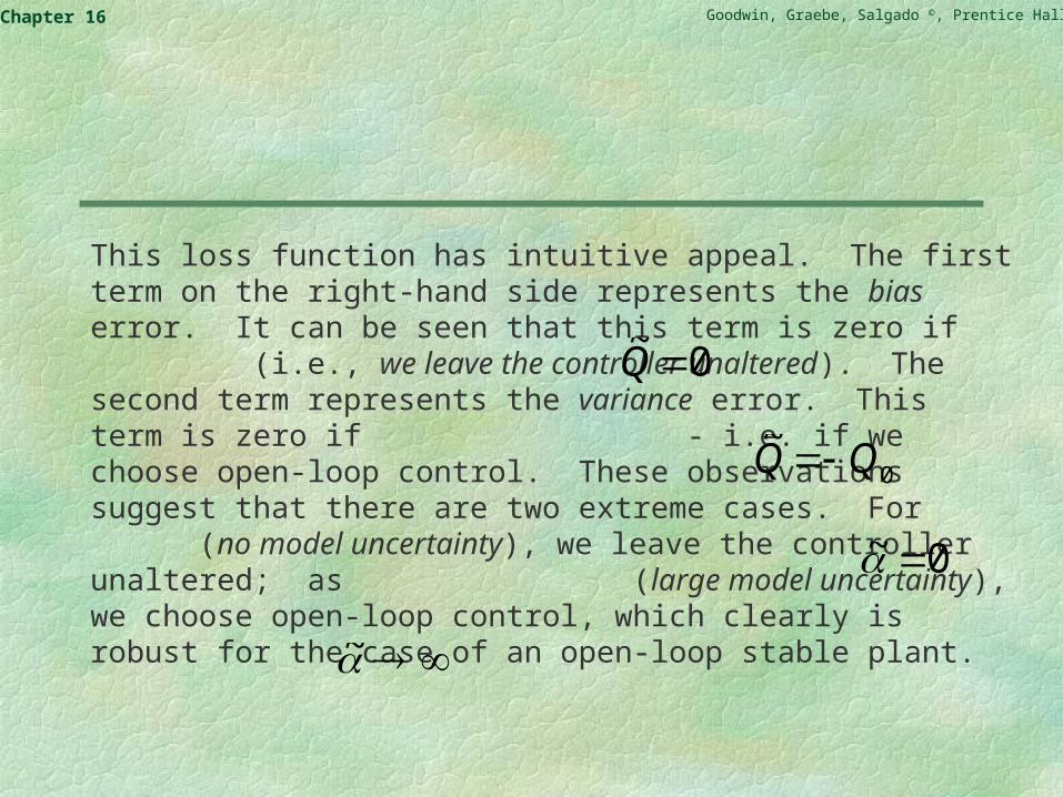
This loss function has intuitive appeal. The first term on the right-hand side represents the bias error. It can be seen that this term is zero if (i.e., we leave the controller unaltered). The second term represents the variance error. This term is zero if - i.e. if we choose open-loop control. These observations suggest that there are two extreme cases. For (no model uncertainty), we leave the controller unaltered; as (large model uncertainty), we choose open-loop control, which clearly is robust for the case of an open-loop stable plant.

0~Q

0~ QQ

0~

~


Intuitive Interpretation (Stable Case)

dGEQQSQGJ e

22

02

022

0~~

Uncertainty

Bias Term Variance Term

Due to using Q Q0

in nominal case00 eGas

Hence: Bias/Variance Trade-Off


The robust design is described in:

Lemma 16.4: Suppose that(i) G0 is strictly proper with no zeros on the imaginary axis

and

(ii) E{G(j)G(-j)} has a spectral factorization.

Then (s)(-s)S0(s)S0(-s) + G0(s)G0(-s) has a spectral factor, which we label H, and the optimal is given by

Q~


Proof: Uses Lemma 16.2 - see the book.


The value of found in Lemma 16.4 gives an optimal trade-off between the bias error and the variance term.

Q~


A final check on robust stability (which is not automatically guaranteed by the algorithm) requires us to check that |G(j)||Q(j) < 1 for all and all likely values of G (j ). A procedure for doing this is described in the book.


Incorporating Integral Action

The methodology given above can be extended to include integral action. Assuming that Q0 provides this property, the final controller will do so as well, if has the form

with strictly proper.

There are a number of ways to enforce this constraint. A particularly simply way is to change the cost function to

Q~

Q ~


Lemma 16.5: Suppose that(I) G0 is strictly proper with no zeros on the imaginary

axis and

(ii) E{G(j)G(-j)} has a spectral factorization as in

Then (s)(-s)S0(s)S0(-s) + G0(s)G0(-s) has a spectral factor, which we label H, and



A Simple Example

Consider a first-order system having constant variance for the model error in the frequency domain:


(a) Without integral-action constraint

In this case, with 1 and 2 appropriate functions of 0, cl, and , we can write


Then there exist A1, A2, A3, and A4, also appropriate functions of 0, cl, and , so that

the optimal is thenQ~


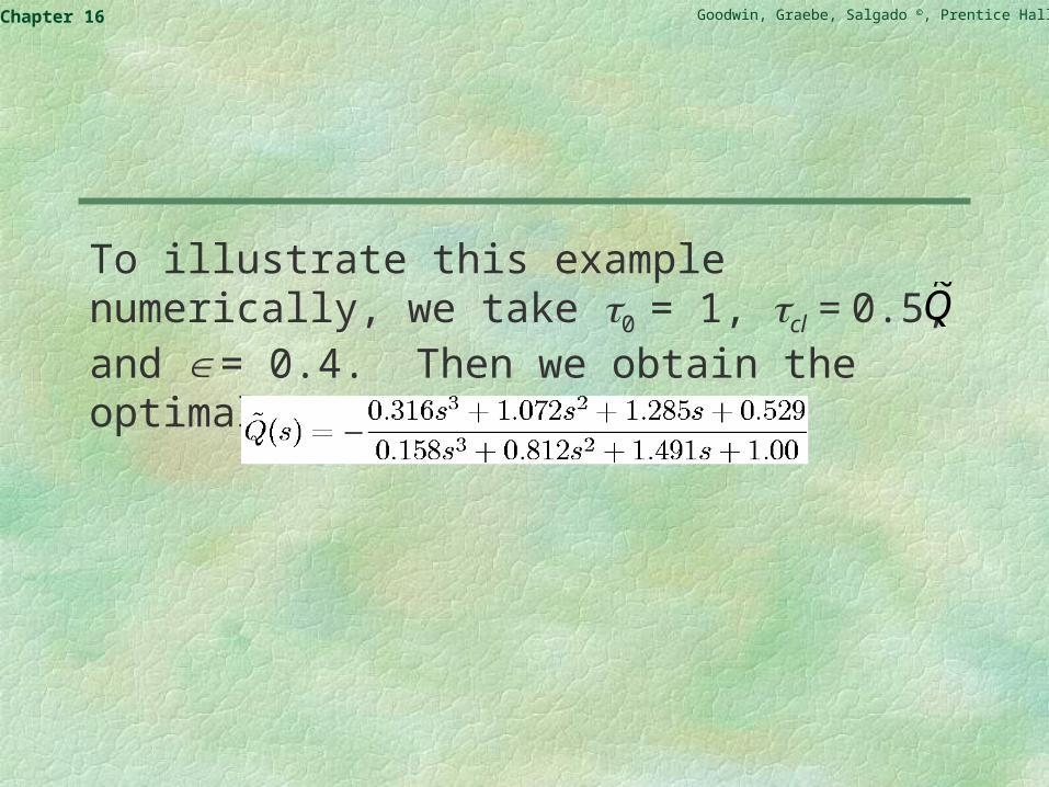
To illustrate this example numerically, we take 0 = 1, cl = 0.5, and = 0.4. Then we obtain the optimal as

Q~


It is interesting to investigate how this optimal contributes to the reduction of the loss function.

Q~


If then

and if the optimal is used, then the total error is J = 4.9, which has a bias error of

and a variance error of

,0)(~ sQ

djQjSJ 2

00 |)()(|

Q~

3.4|~)(| 2

0 dQjG

6.0|)(~)()()(| 2

000 djQjSjQjS


(b) With integral-action constraint

We write

The optimal is given by

scl

B

scl

B

sa

B

sa

B

sclscl

ssclsasa

sclssH

sSsSss sQ

14

2)1(

3

212

111

2)1)(1(

)01)(2(

)21)(11(

)1)(01(0)(

)(0)(0)()( )(

Q~


For the same set of process parameters as above, we obtain the optimal as

and for Q for controller implementation is simply

Q~


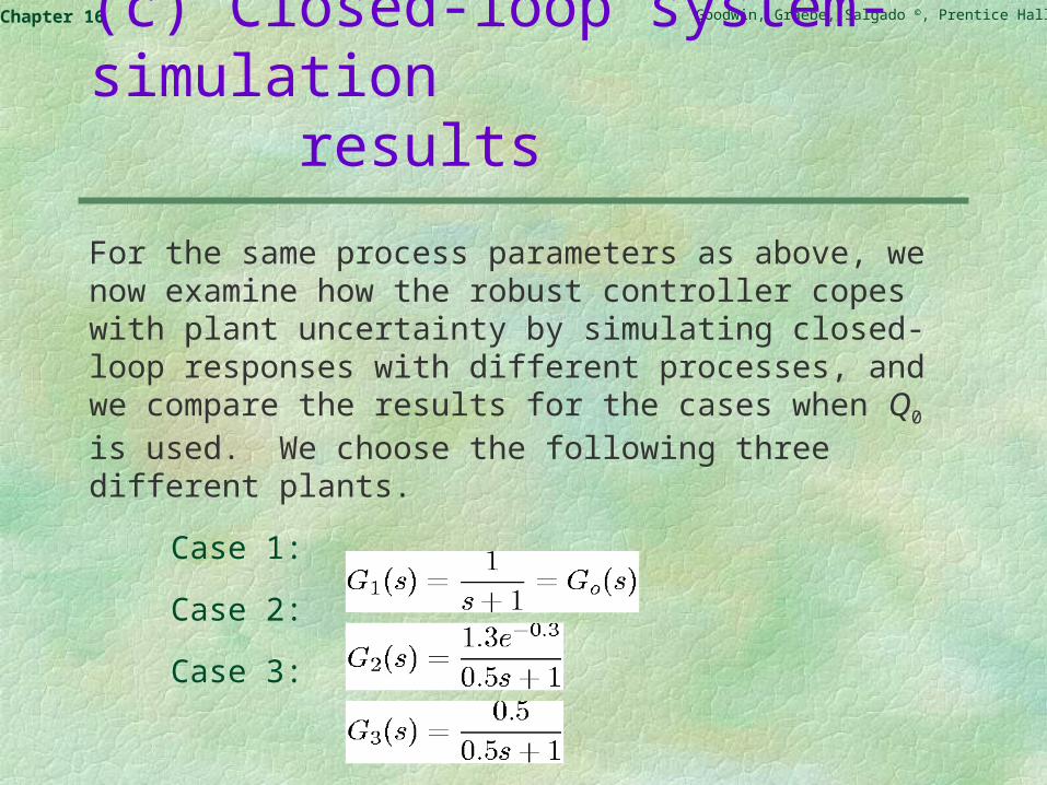
(c) Closed-loop system-simulation results

For the same process parameters as above, we now examine how the robust controller copes with plant uncertainty by simulating closed-loop responses with different processes, and we compare the results for the cases when Q0 is used. We choose the following three different plants.

Case 1:

Case 2:

Case 3:


The frequency responses of the three plants are shown in Figure 16.1. They are within the statistical confidence bounds centered at G0(j) and have standard deviation of .4.0


Figure 16.1: Plane frequency response: Case 1 (solid); case 2 (dashed); case 3 (dotted)


Figures 16.2, 16.3 and 16.4 (see next 3 slides), show the closed-loop responses of the three plants for a unit set-point change, controlled by using C and C0.


Figure 16.2: Closed-loop responses for case 1: when using Q0 (thin line), and when using optimal Q (thick line).


Figure 16.3: Closed-loop responses for case 2: when using Q0 (thin line), and when using optimal Q (thick line)


Figure 16.4: Closed-loop responses for case 3: when using Q0 (thin line), and when using optimal Q (thick line)


Discussion

Case 1: G1(s) = G0(s), so the closed-loop response based on Q0 for this case is the desired response, as specified. The existence of causes degradation in the nominal closed-loop performance, but this degradation is reasonably small, as can be seen from the closeness of the closed-loop responses. This is the price one pays for including a robustness margin aimed at decreasing sensitivity to modeling errors.

Q~


Case 2: There is a large model error between G2(s) and G0(s), shown in figure 16.1. It is seen from Figure 16.3 that, without the compensation of optimal , the closed-loop system and achieves acceptable closed-loop performance in the presence of this large model uncertainty.

Q~


Case 3: Although there is a large model error between G3(s) and G0(s) in the low-frequency region, this model error is less likely to cause instability of the closed-loop system. Figure 16.4 illustrates that the closed-loop response speed, when using the optimal , is indeed slower than the response speed from Q0, but the difference is small.

Q~


Unstable Plant

We next briefly show how the robust design method can be extended to the case of an unstable open-loop plant. As before, we denote the nominal model by , the nominal controller by the nominal sensitivity by S0. We parameterize the modified controller by:

where Q(s) is a stable proper transfer function.

)(0

)(00 )( sA

sBsG )()(

0 )( sLsPsC


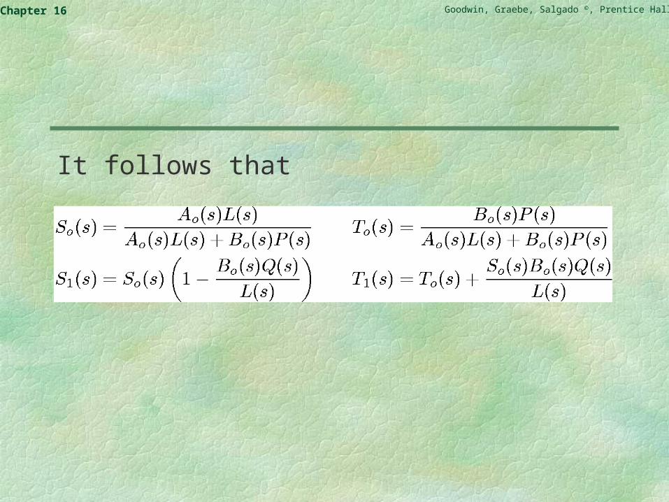
It follows that


Where G(s) and G(s) denote, as usual, the MME and AME, respectively.


As before, we used a weighted measure of S2(s) - S0(s), where the weight is now chosen as

In this case

)()(

)()()(

202)()(0)()(0

)()(0)()(

)()(0)()(0

)()(0)(0022

sGsA

sSsSsW

sPsBsLsA

sQsAsPsL

sPsBsLsAsQsBsA


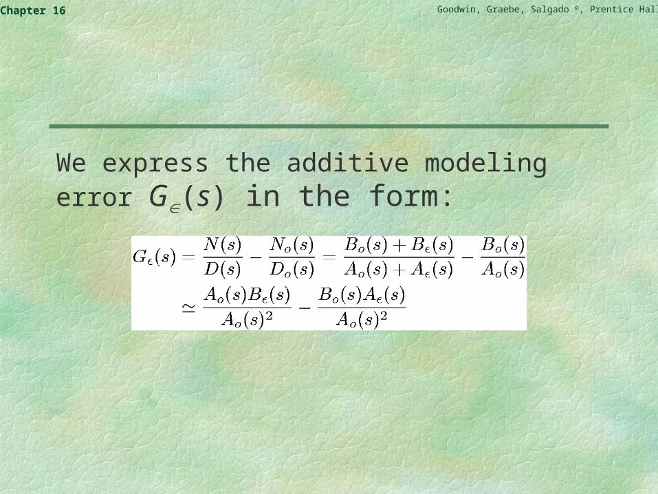
We express the additive modeling error G(s) in the form:


Thus

We can then proceed essentially as in the open-loop stable case.

)()()()(

)()()(

002)()(0)()(0

)()(0)()(

)()(0)()(0

)()(0)(0022

sAsBsBsA

sSsSsW

sPsBsLsA

sQsAsPsL

sPsBsLsAsQsBsA


We illustrate the above ideas below on a practical system. (A laboratory scale heat exchanger). Note that this system is open-loop stable.


Practical Example: Laboratory Heat Exchanger


Motor

Fan

ControllableHeat

SourceHeating Bed

MV

PV

Temperature Sensor

Air Flow

Pictorial View of Heat Exchanger


Approximate Model

1)(

sKe

sGsT

2.2,5.1K

2.0,1.0T

42.0,38.0

Based on physical experiments, the model is of theform:


System Identification

An experiment was carried out to estimate the model. The resultant input/output data is shown on the next slide.


Plant Input-Output Data


Error Bounds

The estimated normal frequency response together with error bounds are shown on the next slide.


Estimated Frequency Response


Nominal Model and Controller

Estimated Model3.212.9

7.334.3)(

2

ss

ssG

Nominal Controllerin Youla Form

7.33100

*10

3.212.9)(

2

2

0

s

sssQ


Stage 2: Robust Control Design

Use Model Error Quantification accounting for noise and undermodelling to modify the controller.

22

234

1.595.9

1.8093.6238.1771.2204.2)(

ss

sssssQ

Result is:


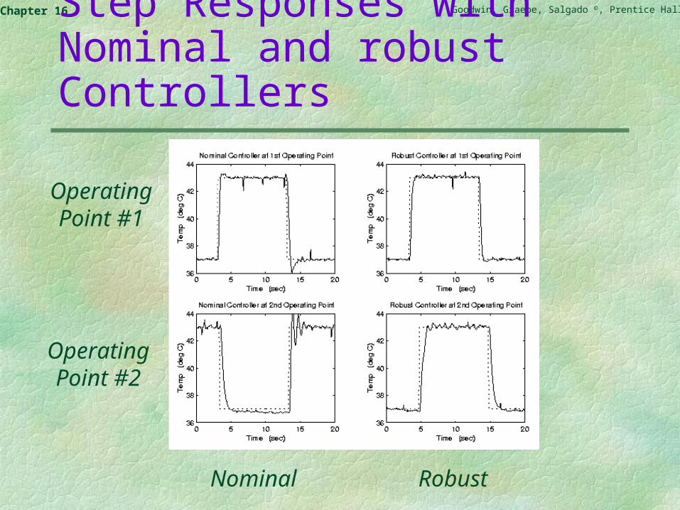
Step Responses with Nominal and robust Controllers

Nominal Robust

OperatingPoint #1

OperatingPoint #2


We see from the above results that the robust controller gives (slightly) less sensitivity of the design to operating point.


Cheap Control Fundamental Limitations

We next use the idea of quadratic optimal design to revisit the issue of fundamental limitations.Consider the standard single-input single-output feedback control loop shown, for example, in Figure 5.1 on the next slide.


Figure 5.1:


Cheap ControlWe will be interested in minimizing the quadratic cost associated with the output response expressed by:

Note that, no account is taken here of the size of the control effort. Hence, this class of problem, is usually called cheap control. It is obviously impractical to allow arbitrarily large control signals. However, by not restricting the control effort, we obtain a benchmark against which other, more realistic, scenarios can be judged. Thus these results give a fundamental limit to the achievable performance.

dttyJ 202

1 )(


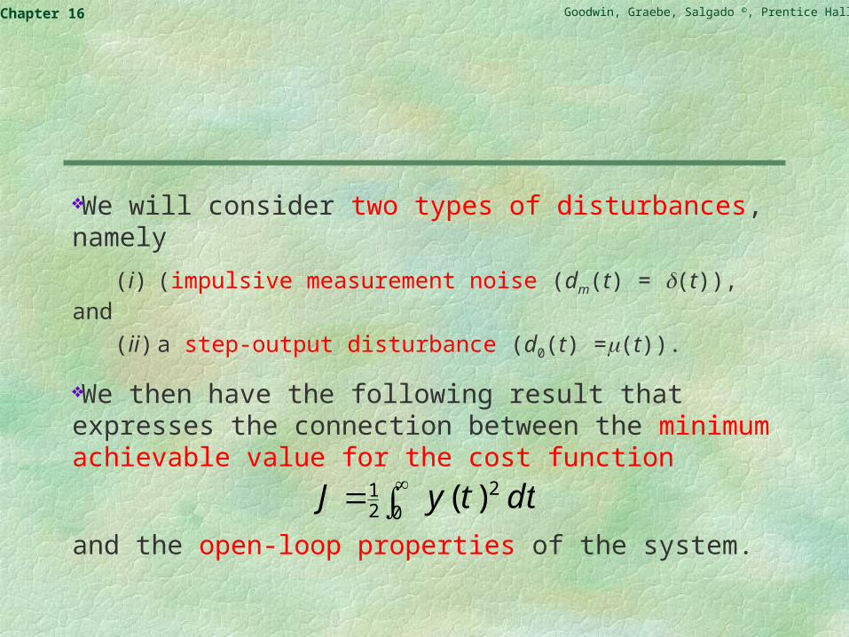
We will consider two types of disturbances, namely

(i) (impulsive measurement noise (dm(t) = (t)), and

(ii) a step-output disturbance (d0(t) =(t)).

We then have the following result that expresses the connection between the minimum achievable value for the cost function

and the open-loop properties of the system.

dttyJ 202

1 )(


Theorem 16.1: Consider the SISO feedback control loop and the cheap control cost function. Then

(i) For impulsive measurement noise, the minimum value for the cost is

where pi, …, pN, denote the open-loop plant poles in the right half plane (unstable), and

N

iipJ

1*


(ii) For a step-output disturbance, the minimum value for the cost is

where c1, …, cM denote the open-loop plant zeros in the right-half plane (unstable).


M

i icJ

1

1*


Frequency-Domain Limitations Revisited

We saw earlier in Chapter 9 that the sensitivity and complementary sensitivity functions satisfied the following integral equations in the frequency domain

(i)

where kh denotes lims 0sH0l(s) and H0l(s) is the open-loop transfer function.

N

ii

h pk

djS1

00 2)(ln

1


(ii)

where kv = lims 0sH0l(s).

There is clearly a remarkable consistency between the right-hand sides of the above equations and the results for cheap control. This is not a coincidence as shown in the following result:

M

i iv ckdjT

100 2

121

)(ln11


Theorem 16.2: Consider the standard SISO control loop in which the open-loop transfer function H0l(s) is strictly proper and H0l(0)-1 = 0 (i.e. there is integral action), then

(i) for impulse measurement noise, the following inequality holds:

where pi, …, pN denote the plant right-half plane poles.

N

ii

h pdjSk

ty1

0002 )(ln1

2)(

21


(ii) for impulse a unit-step output disturbance, then

where ci, …, cM denote the plant right-half plane poles.


M

i iv cdjT

kty

12000

2 1)(ln12

1)(21


Summary

Optimization can often be used to assist with certain aspects of control-system design.

The answer provided by an optimization strategy is only as good as the question that has been asked - that is, how well the optimization criterion captures the relevant design specifications and trade-offs.

Optimization needs to be employed carefully: keep in mind the complex web of trade-offs involved in al control-system design.


Quadratic optimization is a particularly simple strategy and leads to a closed-form solution.

Quadratic optimization can be used for optimal Q synthesis.

We have also shown that quadratic optimization can be used effectively to formulate and solve robust control problems when the model uncertainty is specified in the form of a frequency-domain probabilistic error.


Within this framework, the robust controller biases the nominal solution so as to create conservatism, in view of the expected model uncertainty, while attempting to minimize affecting the achieved performance.

This can be viewed as a formal way of achieving the bandwidth reduction that was discussed earlier as a mechanism for providing a robustness gap in control-system design.

Goodwin, Graebe, Salgado ©, Prentice Hall 2000 Chapter 16 Control Design Based on Optimization.

Documents

Transcript of Goodwin, Graebe, Salgado ©, Prentice Hall 2000 Chapter 16 Control Design Based on Optimization.