© Goodwin, Graebe, Salgado, Prentice Hall 2000 Chapter 9 Frequency Domain Design Limitations.
81
© Goodwin, Graebe, Salgado, Prentice Hall Chapter 9 Chapter 9 Frequency Domain Frequency Domain Design Limitations Design Limitations
-
date post
18-Dec-2015 -
Category
Documents
-
view
234 -
download
0
Transcript of © Goodwin, Graebe, Salgado, Prentice Hall 2000 Chapter 9 Frequency Domain Design Limitations.

©Goodwin, Graebe, Salgado, Prentice Hall 2000Chapter 9
Chapter 9
Frequency Domain Design Frequency Domain Design LimitationsLimitations
©Goodwin, Graebe, Salgado, Prentice Hall 2000Chapter 9
The purpose of this chapter is to develop frequency domain constraints and to explore their interpretations. The results to be presented here have a long and rich history beginning with the seminal work of Bode published in his 1945 book on network synthesis. The results give an alternative view of the fundamental time domain limitations presented in Chapter 8.
©Goodwin, Graebe, Salgado, Prentice Hall 2000Chapter 9
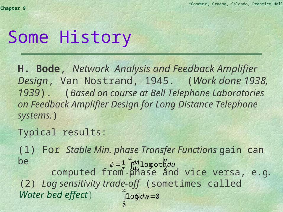
H. Bode, Network Analysis and Feedback Amplifier Design, Van Nostrand, 1945. (Work done 1938, 1939). (Based on course at Bell Telephone Laboratories on Feedback Amplifier Design for Long Distance Telephone systems.)
Typical results:
(1) For Stable Min. phase Transfer Functions gain can be computed from phase and vice versa, e.g.
duu
dudA
2
1 cothlog
(2) Log sensitivity trade-off (sometimes called Water bed effect)
0
0log dwS
Some History

©Goodwin, Graebe, Salgado, Prentice Hall 2000Chapter 9
For historical interest we include (as the next few slides) the first few pages of the book written by Bode
©Goodwin, Graebe, Salgado, Prentice Hall 2000Chapter 9

©Goodwin, Graebe, Salgado, Prentice Hall 2000Chapter 9

©Goodwin, Graebe, Salgado, Prentice Hall 2000Chapter 9

©Goodwin, Graebe, Salgado, Prentice Hall 2000Chapter 9

©Goodwin, Graebe, Salgado, Prentice Hall 2000Chapter 9

©Goodwin, Graebe, Salgado, Prentice Hall 2000Chapter 9
Theme
In Advanced Control, understanding what can and cannot be done (and why) is often more important than producing a specific design.
©Goodwin, Graebe, Salgado, Prentice Hall 2000Chapter 9
The constraints presented here mirror constraints that apply in many other areas, e.g.
Second Law of Thermodynamics Cramer Rao Inequality of Estimation

©Goodwin, Graebe, Salgado, Prentice Hall 2000Chapter 9
Design Constraints in Engineering
(a) It can rule out silly ideas:
For example, consider the following Perpetual Motion Machine?
Generator
(Ruled out by fundamental principle of conservation of energy)
Fan
Motor
Turbine
Examples: First and Second Laws of Thermodynamics
©Goodwin, Graebe, Salgado, Prentice Hall 2000Chapter 9
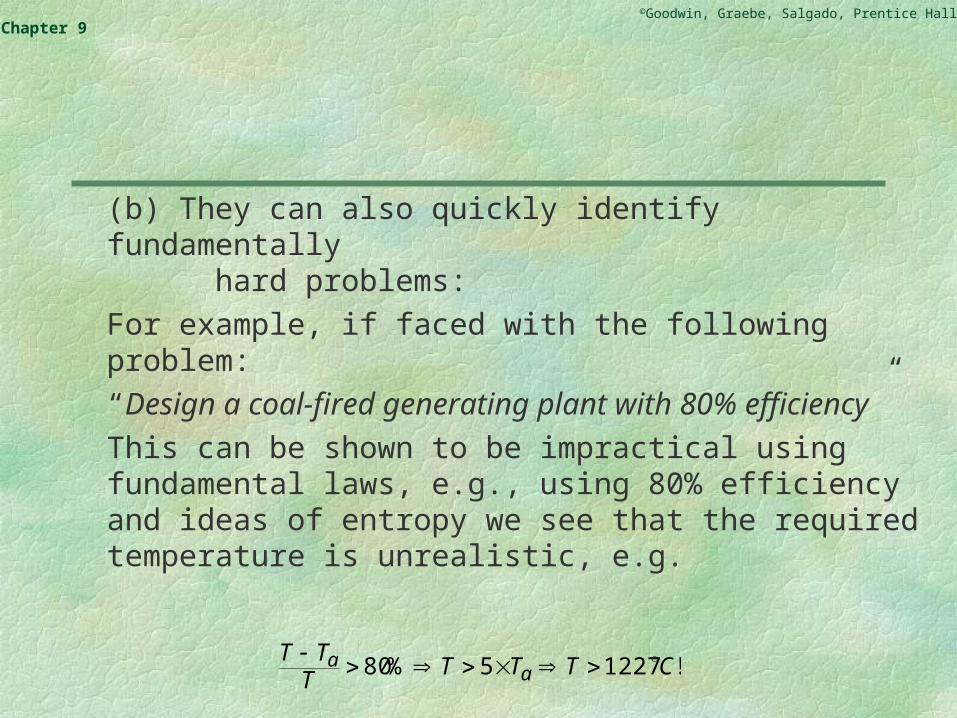
(b) They can also quickly identify fundamentally hard problems:
For example, if faced with the following problem:
“Design a coal-fired generating plant with 80% efficiency”
This can be shown to be impractical using fundamental laws, e.g., using 80% efficiency and ideas of entropy we see that the required temperature is unrealistic, e.g.
!12275%80 CTTTT
TTa
a
©Goodwin, Graebe, Salgado, Prentice Hall 2000Chapter 9
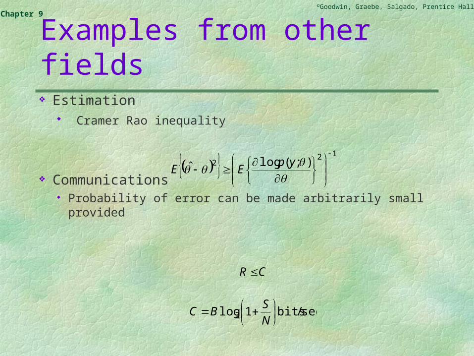
Examples from other fields Estimation
Cramer Rao inequality
Communications Probability of error can be made arbitrarily small provided
12
2 );(logˆ
yp
EE
CR
sec/bits1log2
NS
BC

©Goodwin, Graebe, Salgado, Prentice Hall 2000Chapter 9
One of the best known results is that for a stable minimum phase system, the phase is uniquely determined by the magnitude and vice versa. The exact formula is given on the next slide.

©Goodwin, Graebe, Salgado, Prentice Hall 2000Chapter 9
Weighting Function
2cothlog
|)(|log1)( 00
udu
ejHd u
Thus, the slope of the magnitude curve in the vicinity of0, say c, determines the phase (0):
222cothlog)(
2
0
ccduuc

©Goodwin, Graebe, Salgado, Prentice Hall 2000Chapter 9
Here we study the fundamental design constraints that apply to feedback systems of the type illustrated below
The constraints we develop apply to frequency domain integrals of the sensitivity function and complementary sensitivity function.
C G+
-

©Goodwin, Graebe, Salgado, Prentice Hall 2000Chapter 9
Conceptual Background
Before delving into technical details, we first review the conceptual nature of the results to be presented.
The simplest (and perhaps best known) result is that, for an open loop stable plant, the integral of the logarithm of the closed loop sensitivity is zero; i.e.
Now we know that the logarithm function has the property that it is negative if |S0| < 1 and it is positive if |S0| > 1.
0 0 0|)(|ln dwjwS

©Goodwin, Graebe, Salgado, Prentice Hall 2000Chapter 9
Graphical interpretation of the area formula
Typical Nyquist plot for a stable rational transfer function, L, of relative degree two:
Note that S(j)-1 = 1 + L(j) is the vector from the -1 point to the point on the Nyquist plot corresponding to the frequency .
It is clear from the plot that frequencies where |S(jw)| < 1 are balanced by frequencies where |S(jw)| > 1.

©Goodwin, Graebe, Salgado, Prentice Hall 2000Chapter 9
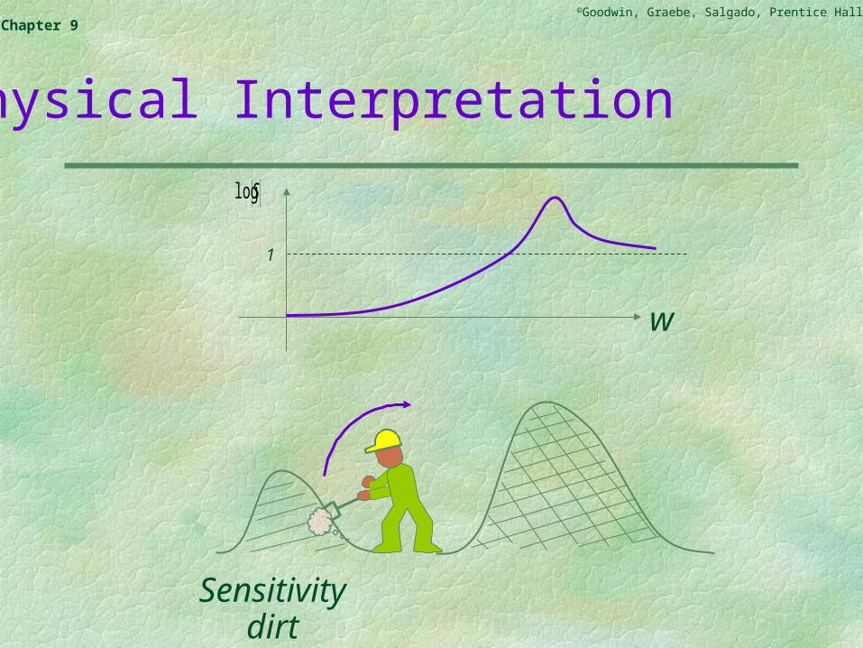
The above result implies that set of frequencies over which sensitivity reduction occurs (i.e. where |S0| < 1) must be matched by a set of frequencies over which sensitivity magnification occurs (i.e. where |S0| > 1).
This has been given a nice (cartoon like) interpretation as thinking of sensitivity as a pile of dirt. If we remove dirt from one set of frequencies, then it piles up at other frequencies. This is conceptually illustrated on the next slide.
©Goodwin, Graebe, Salgado, Prentice Hall 2000Chapter 9
Sensitivitydirt
1
Slog
w
Physical Interpretation

©Goodwin, Graebe, Salgado, Prentice Hall 2000Chapter 9
We will show in the sequel that the above sensitivity trade-off is actually made more difficult if there are either (or both)
Right half plane open loop zeros Right half plane open loop poles
Notice that these results hold irrespective of how the control system is designed; i.e. they are fundamental constraints that apply to all feedback solutions.

©Goodwin, Graebe, Salgado, Prentice Hall 2000Chapter 9
Indeed, it will turn out that to avoid large frequency domain sensitivity peaks it is necessary to limit the range of sensitivity reduction to be:
(i) less than any right half plane open loop zero
(ii) greater than any right half plane open loop pole.

©Goodwin, Graebe, Salgado, Prentice Hall 2000Chapter 9
This begs the question - “What happens if there is a right half plane open loop zero having smaller magnitude than a right half plan open loop pole?”
Clearly the requirements specified on the previous slide are then mutually incompatible. The consequence is that large sensitivity peaks are unavoidable and, as a result, poor feedback performance is inevitable.
An example precisely illustrating this conclusion will be presented later.

©Goodwin, Graebe, Salgado, Prentice Hall 2000Chapter 9
We begin with Bode’s integral constraint on sensitivity. This is a formal statement of the result discussed above at a conceptual level; namely
0 0 0|)(|ln dwjwS
©Goodwin, Graebe, Salgado, Prentice Hall 2000Chapter 9
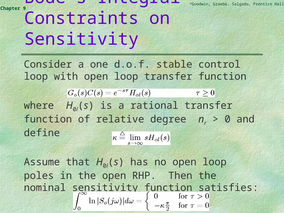
Bode’s Integral Constraints on SensitivityConsider a one d.o.f. stable control loop with open loop transfer function
where H0l(s) is a rational transfer function of relative degree nr > 0 and define
Assume that H0l(s) has no open loop poles in the open RHP. Then the nominal sensitivity function satisfies:
©Goodwin, Graebe, Salgado, Prentice Hall 2000Chapter 9
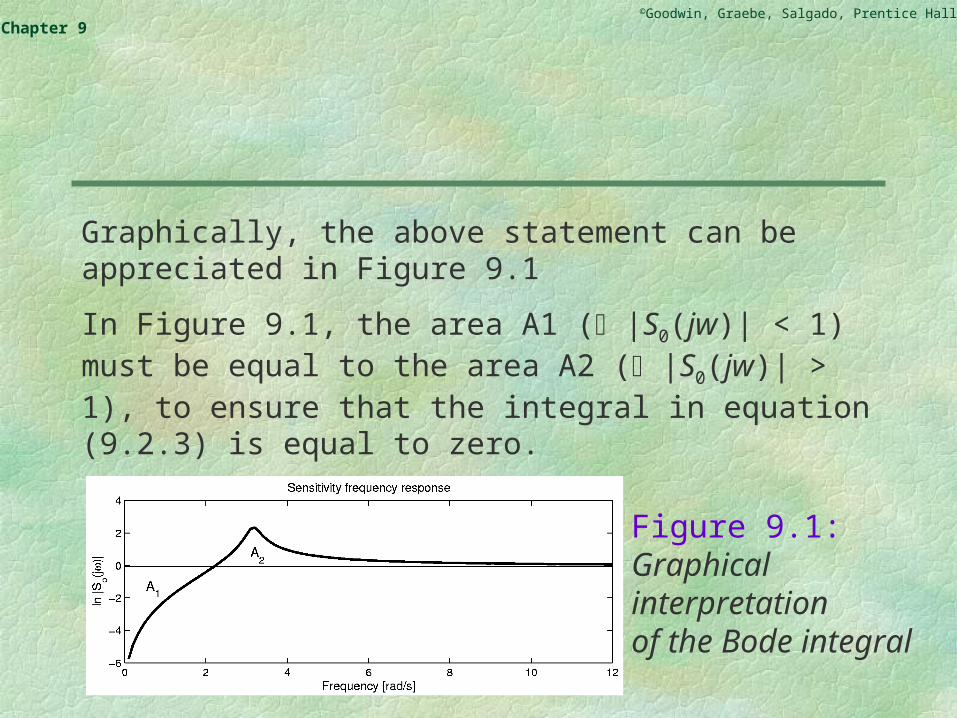
Graphically, the above statement can be appreciated in Figure 9.1
In Figure 9.1, the area A1 ( |S0(jw)| < 1) must be equal to the area A2 ( |S0(jw)| > 1), to ensure that the integral in equation (9.2.3) is equal to zero.
Figure 9.1:Graphicalinterpretationof the Bode integral

©Goodwin, Graebe, Salgado, Prentice Hall 2000Chapter 9
Proof
We will not give a formal proof of this result. Suffice to say it is an elementary consequence of the well known Cauchy integral theorem of complex variable theory - see the book for details.
©Goodwin, Graebe, Salgado, Prentice Hall 2000Chapter 9
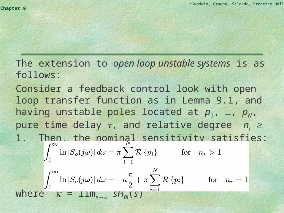
The extension to open loop unstable systems is as follows:
Consider a feedback control look with open loop transfer function as in Lemma 9.1, and having unstable poles located at p1, …, pN, pure time delay , and relative degree nr 1. Then, the nominal sensitivity satisfies:
where = lims sH0l(s)

©Goodwin, Graebe, Salgado, Prentice Hall 2000Chapter 9
Observations
We see from the above results that with open loop RHP poles, the integral of log sensitivity is required to be greater than zero (previously) it had to be zero. This makes sensitivity minimization more difficult.
©Goodwin, Graebe, Salgado, Prentice Hall 2000Chapter 9
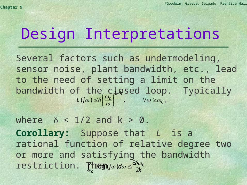
Design Interpretations
Several factors such as undermodeling, sensor noise, plant bandwidth, etc., lead to the need of setting a limit on the bandwidth of the closed loop. Typically
where < 1/2 and k > 0.
Corollary: Suppose that L is a rational function of relative degree two or more and satisfying the bandwidth restriction. Then
,,)(1
c
kcjL
.2
3)(log
kdjS c
c
©Goodwin, Graebe, Salgado, Prentice Hall 2000Chapter 9
The above result shows that the area of the tail of the Bode sensitivity integral over the infinite frequency range [c, ) is limited.
©Goodwin, Graebe, Salgado, Prentice Hall 2000Chapter 9
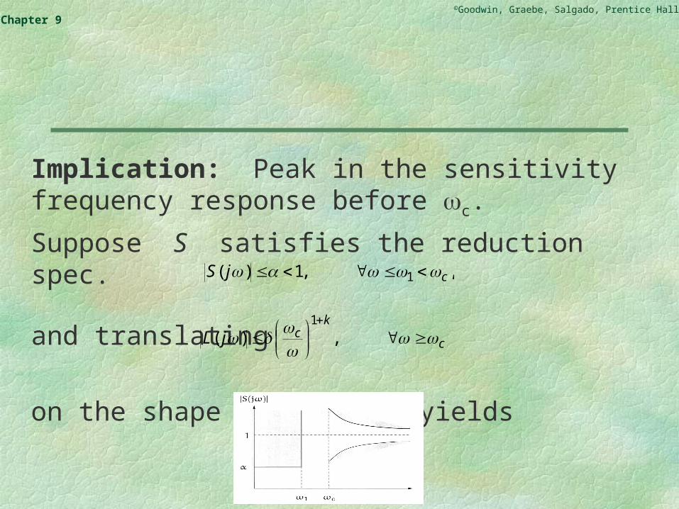
Implication: Peak in the sensitivity frequency response before c.
Suppose S satisfies the reduction spec.
and translating
on the shape of |S(jw)| yields
,,1)( 1 cjS
c
kcjL
,)(
1

©Goodwin, Graebe, Salgado, Prentice Hall 2000Chapter 9
Now, using the bounds (2) and (1) in the Bode sensitivity integral, it is easy to show that
Then, the larger the area of sensitivity reduction (i.e., small and/or 1 close to c ) will necessarily result in a large peak in the range(1, c).
Hence, the Bode sensitivity integral imposes a design trade-off when natural bandwidth constraints are assumed for the closed-loop system.
.
231log1)(logsup 1
1,1
kpjS c
zpcsc

©Goodwin, Graebe, Salgado, Prentice Hall 2000Chapter 9
Example
The inequality
can be used to derive a lower bound on the closed-loop bandwidth in terms of the sum of open-loop unstable poles. Let
.
231log1)(logsup 1
1,1
kpjS c
zpcsc
.11 ck
©Goodwin, Graebe, Salgado, Prentice Hall 2000Chapter 9
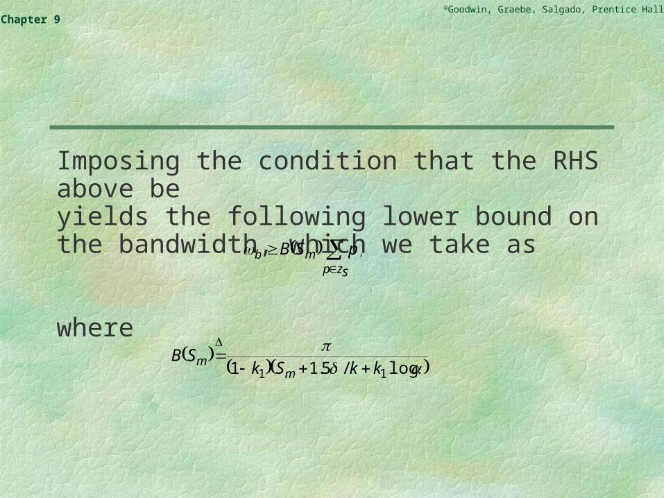
Imposing the condition that the RHS above beyields the following lower bound on the bandwidth, which we take as
where
szp
mb pSB ,
.log/5.11 11
kkSk
SBm
m
©Goodwin, Graebe, Salgado, Prentice Hall 2000Chapter 9
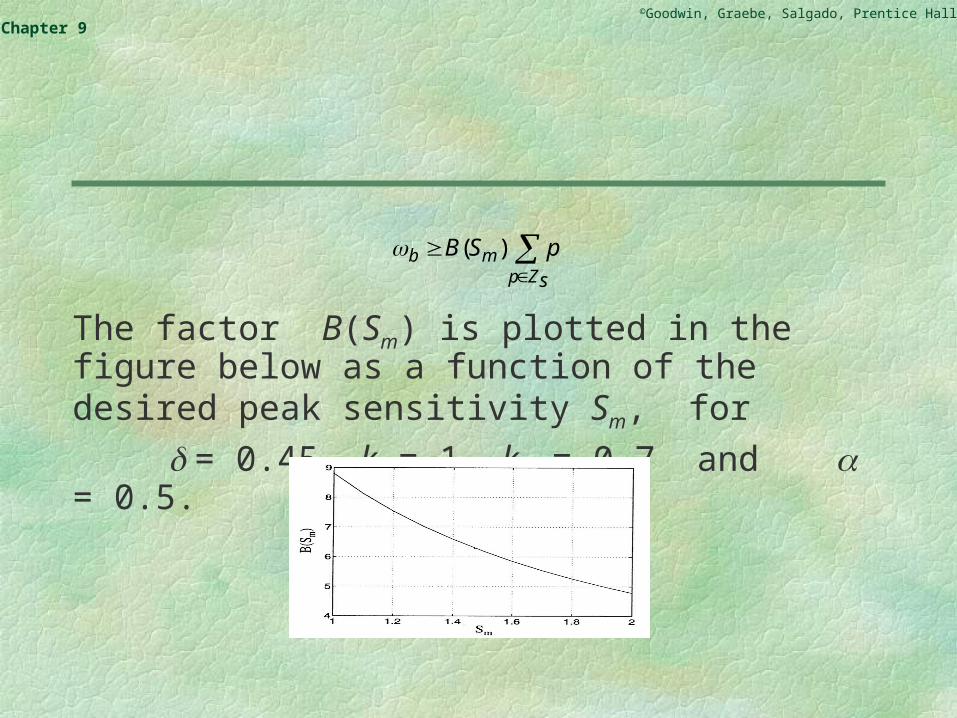
The factor B(Sm) is plotted in the figure below as a function of the desired peak sensitivity Sm, for
= 0.45, k = 1, k1 = 0.7 and = 0.5.
sZp
mb pSB )(

©Goodwin, Graebe, Salgado, Prentice Hall 2000Chapter 9
For example, an open-loop unstable system having relative degree two requires a bandwidth of at least 6.5 times the sum of its ORHP poles if it is desired that S be smaller than 1/2 over 70% of the closed-loop bandwidth while keeping the lower bound on the peak sensitivity smaller than Sm = 2 .

©Goodwin, Graebe, Salgado, Prentice Hall 2000Chapter 9
We next turn to dual results that hold for complementary sensitivity reduction.
©Goodwin, Graebe, Salgado, Prentice Hall 2000Chapter 9
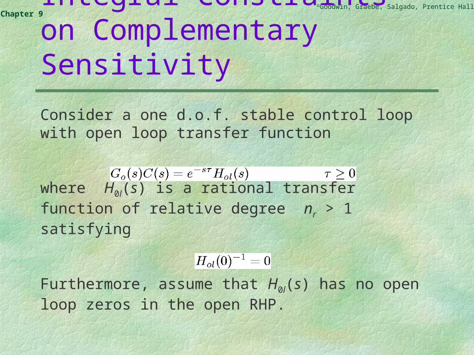
Integral Constraints on Complementary Sensitivity
Consider a one d.o.f. stable control loop with open loop transfer function
where H0l(s) is a rational transfer function of relative degree nr > 1 satisfying
Furthermore, assume that H0l(s) has no open loop zeros in the open RHP.

©Goodwin, Graebe, Salgado, Prentice Hall 2000Chapter 9
Then the nominal complementary sensitivity function satisfies:
where kv is the velocity constant of the open loop transfer function satisfying:
vk2
)(1lim
)(lim1
00
0
ssH
dssdT
k
ls
sv
©Goodwin, Graebe, Salgado, Prentice Hall 2000Chapter 9
As for sensitivity reduction, the trade-off described above becomes harder in the presence of open loop RHP singularities. For the case of complementary sensitivity reduction, it is the open loop RHP zeros that influence the result. The formal result is stated on the next slide.

©Goodwin, Graebe, Salgado, Prentice Hall 2000Chapter 9
Assume that H0l(s) has open loop zeros in the open RHP, located at c1, c2, …, cM, then
M
i vi kcdwjwT
w 100 2 2
1|)(|ln1
©Goodwin, Graebe, Salgado, Prentice Hall 2000Chapter 9
We next turn to a set of frequency domain integrals which are closely related to the Bode type integrals presented above but which allow us to consider RHP open loop poles and zeros simultaneously. These integrals are usually called Poisson type integral constraints.
©Goodwin, Graebe, Salgado, Prentice Hall 2000Chapter 9
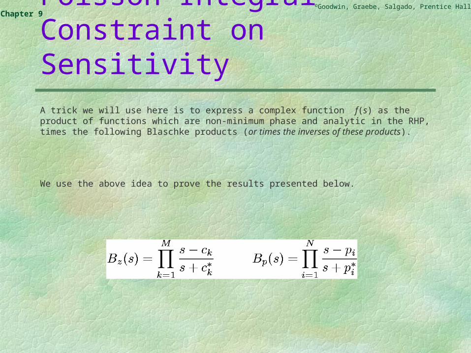
Poisson Integral Constraint on Sensitivity
A trick we will use here is to express a complex function f(s) as the product of functions which are non-minimum phase and analytic in the RHP, times the following Blaschke products (or times the inverses of these products).
We use the above idea to prove the results presented below.
©Goodwin, Graebe, Salgado, Prentice Hall 2000Chapter 9
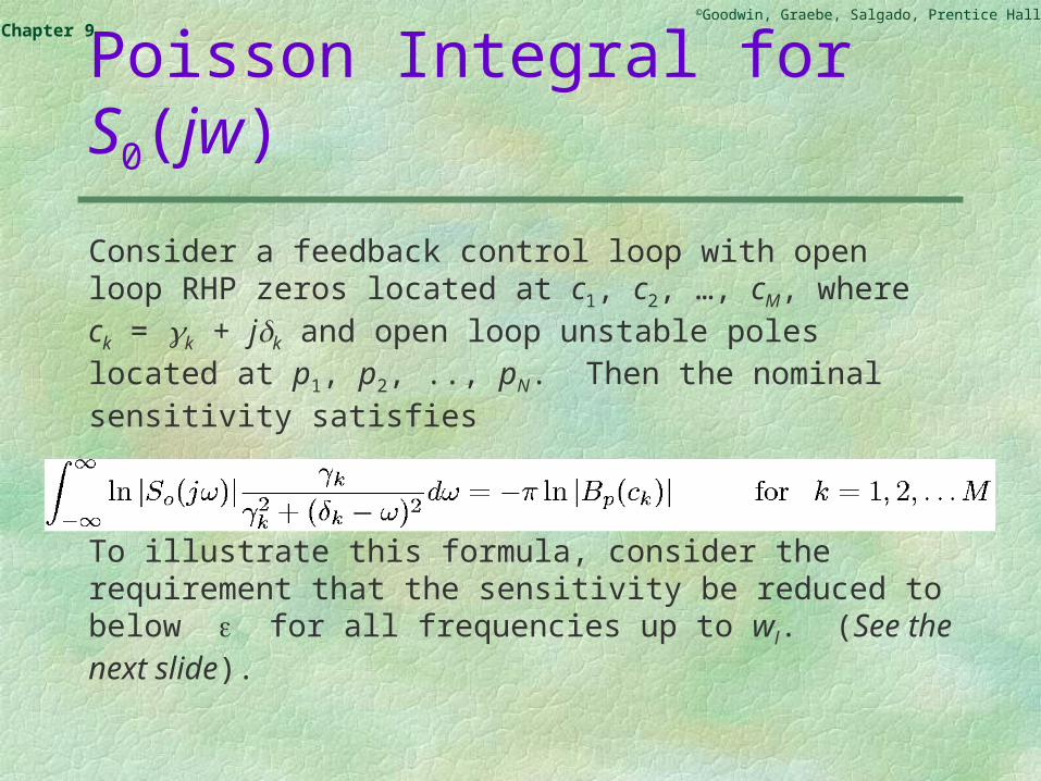
Poisson Integral for S0(jw)
Consider a feedback control loop with open loop RHP zeros located at c1, c2, …, cM, where ck = k + jk and open loop unstable poles located at p1, p2, .., pN. Then the nominal sensitivity satisfies
To illustrate this formula, consider the requirement that the sensitivity be reduced to below for all frequencies up to wl. (See the next slide).

©Goodwin, Graebe, Salgado, Prentice Hall 2000Chapter 9
Figure 9.2: Design specification for |S0(jw)|
Notional closed loop bandwidth
©Goodwin, Graebe, Salgado, Prentice Hall 2000Chapter 9
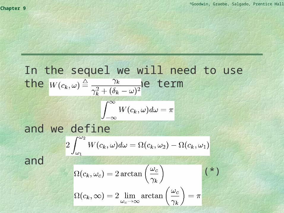
In the sequel we will need to use the integral of the term
and we define
and(*)
©Goodwin, Graebe, Salgado, Prentice Hall 2000Chapter 9
Discussion(i) Consider the plot of sensitivity versus frequency shown on the
previous slide. Say we were to require the closed loop bandwidth to be greater than the magnitude of a right half plane (real) zero. In terms of the notation used in the figure, this would imply wl > k. We can then show using the Poisson formula that there is necessarily a very large sensitivity peak occurring beyond wl. To estimate this peak, assume that wl = 2k and take in Figure 6.2 as 0.3. Then, without considering the effect of any possible open loop unstable pole, the sensitivity peak will be bounded below as follows:
©Goodwin, Graebe, Salgado, Prentice Hall 2000Chapter 9
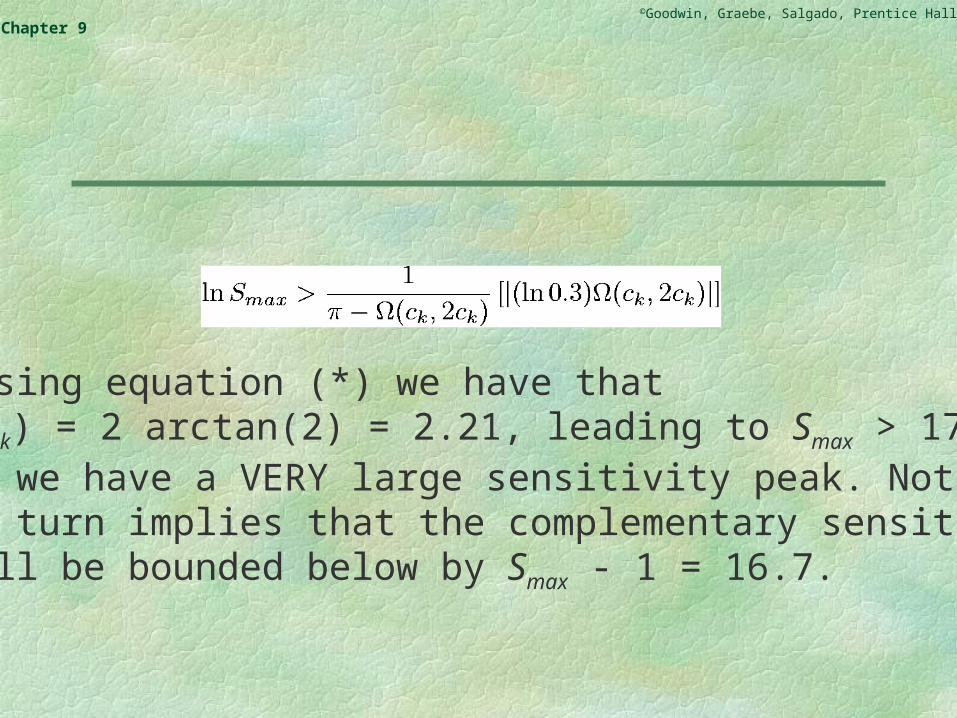
Then, using equation (*) we have that (ck, 2ck) = 2 arctan(2) = 2.21, leading to Smax > 17.7. That is we have a VERY large sensitivity peak. Note that this in turn implies that the complementary sensitivity peak will be bounded below by Smax - 1 = 16.7.
©Goodwin, Graebe, Salgado, Prentice Hall 2000Chapter 9
(ii) The observation in (i) is consistent with the analysis carried out in Chapter 8. In both cases the conclusion is that the closed loop bandwidth should not exceed the magnitude of the smallest RHP open loop zero. The penalty for not following this guideline is that a very large sensitivity peak will occur, leading to fragile loops (non robust) and large undershoots and overshoots.

©Goodwin, Graebe, Salgado, Prentice Hall 2000Chapter 9
(iii) In the presence of unstable open loop poles, the problem is compounded through the presence of the factor |ln|Bp(ck)||. This factor grows without bound when one RHP zero approaches an unstable open loop pole.
©Goodwin, Graebe, Salgado, Prentice Hall 2000Chapter 9
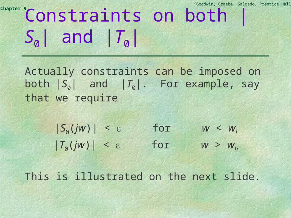
Constraints on both |S0| and |T0|
Actually constraints can be imposed on both |S0| and |T0|. For example, say that we require
|S0(jw)| < for w < wl
|T0(jw)| < for w > wh
This is illustrated on the next slide.

©Goodwin, Graebe, Salgado, Prentice Hall 2000Chapter 9
Figure 9.3: Design specifications for |S0(jw)| and |T0(jw)|
©Goodwin, Graebe, Salgado, Prentice Hall 2000Chapter 9
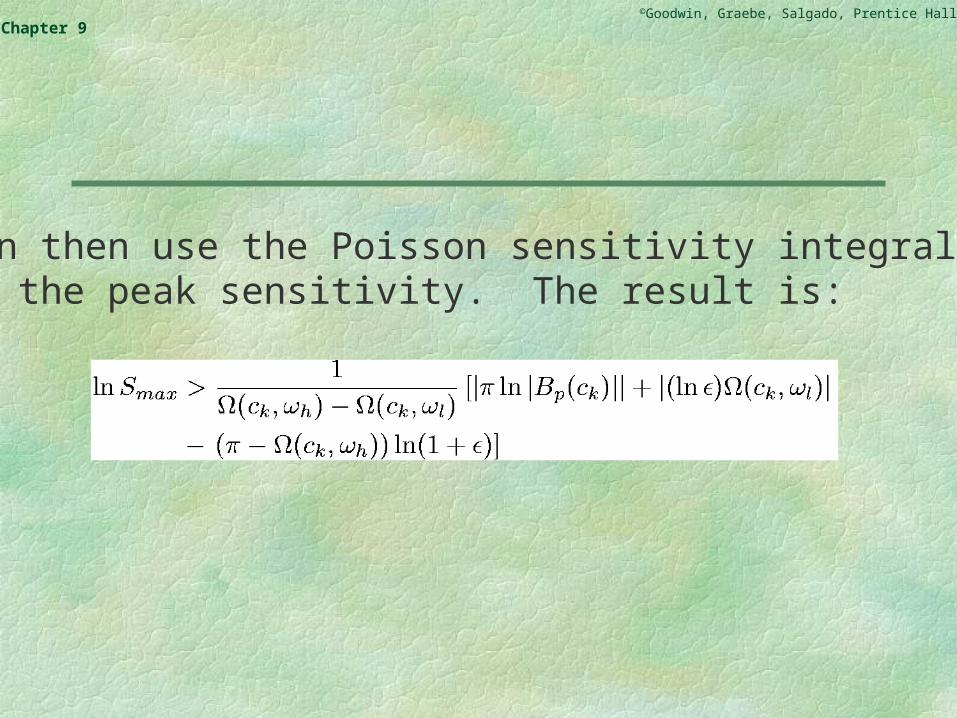
We can then use the Poisson sensitivity integral tobound the peak sensitivity. The result is:

©Goodwin, Graebe, Salgado, Prentice Hall 2000Chapter 9
We next turn to the dual Poisson integral constraints that hold for the complementary sensitivity function. The formal result is stated on the next slide.

©Goodwin, Graebe, Salgado, Prentice Hall 2000Chapter 9
Poisson Integral Constraint on Complementary Sensitivity
Poisson integral for T0(jw). Consider a feedback control loop with delay 0, and having open loop unstable poles located at p1, p2, …, pN, where pi = i + ji and open loop zeros in the open RHP, located at c1, c2, …, cM. Then,

©Goodwin, Graebe, Salgado, Prentice Hall 2000Chapter 9
Say that we require that |T0| < for w > wh. Then it follows from the above result that the peak value of the complementary sensitivity will be bounded from below as follows:

©Goodwin, Graebe, Salgado, Prentice Hall 2000Chapter 9
Discussion
(i) We see that the lower bound on the complementary sensitivity peak is larger for systems with pure delays, and the influence of a delay increases for unstable poles which are far away from the imaginary axis, i.e. large i.
(ii) The peak, Tmax, grows unbounded when a RHP zero approaches an unstable pole, since then |ln|Bz(pi)|| grows unbounded.

©Goodwin, Graebe, Salgado, Prentice Hall 2000Chapter 9
(iii) Say that we ask that the closed loop bandwidth be much smaller than the magnitude of a right half plane (real) pole. In terms of the notation used above, we would then have wh << i. Under these conditions, (pi, wh) will be very small, leading to a very large complementary sensitivity peak. This is an unacceptable result. Thus we conclude that the closed loop bandwidth should be greater than any RHP open loop poles.

©Goodwin, Graebe, Salgado, Prentice Hall 2000Chapter 9
We note that this is consistent with the results based on time domain analysis presented in Chapter 8. There it was shown that, when the closed loop bandwidth is not greater than an open loop RHP pole, large time domain overshoot will occur.

©Goodwin, Graebe, Salgado, Prentice Hall 2000Chapter 9
Example of Design Trade-offs
We will illustrate the application of the above ideas by considering the inverted pendulum problem.
Such systems exist in many universities and are used to illustrate control principles. The key idea is to balance a rod on top of a moving cart (similar to balancing a broom on one’s hand). A photograph of a real inverted pendulum system (at the University of Newcastle) is shown on the next slide.

©Goodwin, Graebe, Salgado, Prentice Hall 2000Chapter 9
Example of an Inverted Pendulum

©Goodwin, Graebe, Salgado, Prentice Hall 2000Chapter 9
We will consider the following control problem:
Sensors:
We measure the position of the cart (but NOT the angle of the pendulum)
Actuators:
We can apply forces to the cart.
Goal:
We want to position the cart at some location plus have the pendulum balancing vertically.

©Goodwin, Graebe, Salgado, Prentice Hall 2000Chapter 9
Inverted pendulum without angle measurement
A schematic diagram of the system is shown below:
Figure 9.4: Inverted pendulum
©Goodwin, Graebe, Salgado, Prentice Hall 2000Chapter 9
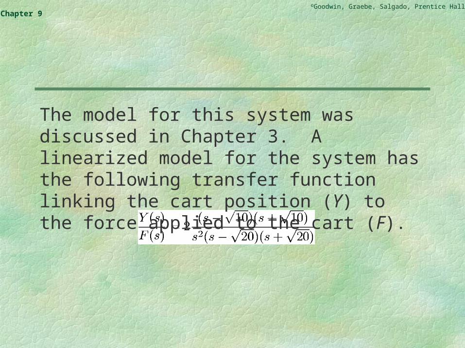
The model for this system was discussed in Chapter 3. A linearized model for the system has the following transfer function linking the cart position (Y) to the force applied to the cart (F).
©Goodwin, Graebe, Salgado, Prentice Hall 2000Chapter 9
We note that this system has an open loop RHP zero at 10 an open loop RHP pole at 20
We observe that the RHP pole has greater magnitude than the RHP zero. The reader is reminded of the comments made in the following two slides which appeared in the earlier part of this chapter.

©Goodwin, Graebe, Salgado, Prentice Hall 2000Chapter 9
Indeed, it will turn out that to avoid large frequency domain sensitivity peaks it is necessary to limit the range of sensitivity reduction to be:
(i) less than any right half plane open loop zero
(ii) greater than any right half plane open loop pole.

©Goodwin, Graebe, Salgado, Prentice Hall 2000Chapter 9
This begs the question - “What happens if there is a right half plane open loop zero having smaller magnitude than a right half plan open loop pole?”
Clearly the requirements specified on the previous slide are then mutually incompatible. The consequence is that large sensitivity peaks are unavoidable and, as a result, poor feedback performance is inevitable.
An example precisely illustrating this conclusion will be presented later.

©Goodwin, Graebe, Salgado, Prentice Hall 2000Chapter 9
We will show formally using the Poisson integral formulae that the predictions made above are indeed true for this example.
©Goodwin, Graebe, Salgado, Prentice Hall 2000Chapter 9
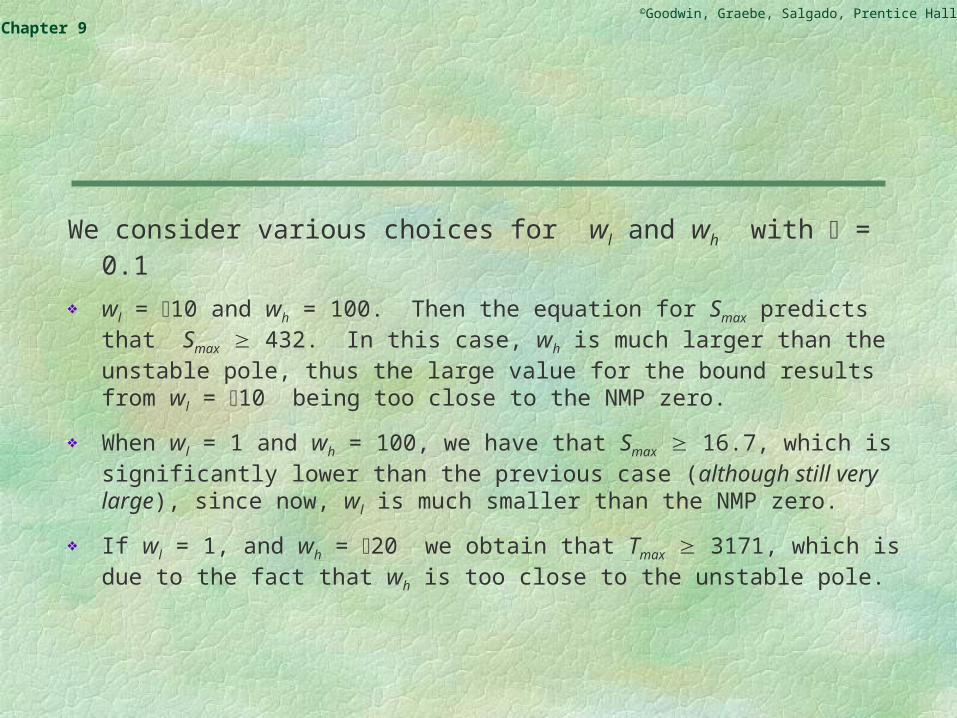
We consider various choices for wl and wh with = 0.1
wl = 10 and wh = 100. Then the equation for Smax predicts that Smax 432. In this case, wh is much larger than the unstable pole, thus the large value for the bound results from wl = 10 being too close to the NMP zero.
When wl = 1 and wh = 100, we have that Smax 16.7, which is significantly lower than the previous case (although still very large), since now, wl is much smaller than the NMP zero.
If wl = 1, and wh = 20 we obtain that Tmax 3171, which is due to the fact that wh is too close to the unstable pole.

©Goodwin, Graebe, Salgado, Prentice Hall 2000Chapter 9
If wl = 1, and wh = 3 we obtain that Tmax 7.2 105. This huge lower bound originates from two facts: firstly wh is lower than the unstable pole, and secondly, wl and wh are very close.
We thus see that, no matter how we try to allocate wl and wh, large sensitivity peaks occur. Thus this system seems to be extremely difficult to control.

©Goodwin, Graebe, Salgado, Prentice Hall 2000Chapter 9
The above conclusion is not unreasonable. (The reader should try balancing a broom on one’s hand with one’s eyes shut!)
The key point is that the angle of the pendulum is not measured.
In a later chapter we will see that a simple change in the architecture made possible by providing a measurement of the angle turns this near impossible control problem into a very easy one (see also the discussion on the web site).

©Goodwin, Graebe, Salgado, Prentice Hall 2000Chapter 9
To illustrate just how hard this problem is, (when the angle is not measured) we designed a stabilizing controller as shown on the next slide.
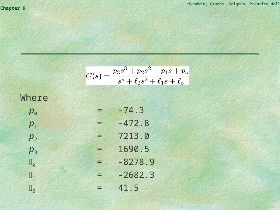
©Goodwin, Graebe, Salgado, Prentice Hall 2000Chapter 9
Wherep0 = -74.3
p1 = -472.8
p2 = 7213.0
p3 = 1690.5
0 = -8278.9
1 = -2682.3
2 = 41.5

©Goodwin, Graebe, Salgado, Prentice Hall 2000Chapter 9
Using the Poisson integrals, we predict
Smax 6.34
Tmax 7.19
The actual sensitivity plots are shown on the next page. These show that these lower bounds are indeed exceeded by the specified controller presented on the previous slide.

©Goodwin, Graebe, Salgado, Prentice Hall 2000Chapter 9
Figure 9.5: Sensitivities for the inverted pendulum
©Goodwin, Graebe, Salgado, Prentice Hall 2000Chapter 9
Summary
One class of design constraints are those which hold at a particular frequency.
Thus we can view the law S(jw) = 1 - T(jw) on a frequency by frequency basis. It states that no single frequency can be removed from both the sensitivity, S(jw), and complementary sensitivity, T(jw).
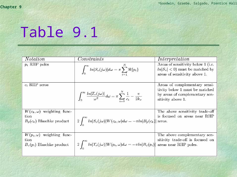
There is, however, an additional class of design considerations, which results from so called frequency domain integral constraints, see Table 9.1.
©Goodwin, Graebe, Salgado, Prentice Hall 2000Chapter 9
Table 9.1
©Goodwin, Graebe, Salgado, Prentice Hall 2000Chapter 9
This chapter explores the origin and nature of these integral constraints and derives their implications for control system performance: The constraints are a direct consequence of the requirement that all sensitivity
functions must be stable; mathematically, this means that the sensitivities are required to be analytic in the
right half complex plane; results from analytic function theory then show, that this requirement necessarily
implies weighted integrals of the frequency response necessarily evaluate to a constant;
hence, if one designs a controller to have low sensitivity in a particular frequency range, then the sensitivity will necessarily increase at other frequencies-a consequence of the weighted integral always being a constant; this phenomenon has also been called the water bed effect (pushing down on the water bed in one area, raises it somewhere else).
©Goodwin, Graebe, Salgado, Prentice Hall 2000Chapter 9
These trade-offs show that systems become increasingly difficult to control as Unstable zeros become slower
Unstable poles become faster
Time delays get bigger.