Going beyond simple sample size calculations: a practitioner's guide

IFS Working Paper W15/17

Brendon McConnellMarcos Vera-Hernández

The Institute for Fiscal Studies (IFS) is an independent research institute whose remit is to carry out rigorous economic research into public policy and to disseminate the findings of this research. IFS receives generous support from the Economic and Social Research Council, in particular via the ESRC Centre for the Microeconomic Analysis of Public Policy (CPP). The content of our working papers is the work of their authors and does not necessarily represent the views of IFS research staff or affiliates.

Going Beyond Simple Sample Size Calculations: a

Practitioner’s Guide

Brendon McConnell and Marcos Vera-Hernandez∗

September 24, 2015

Abstract

Basic methods to compute required sample sizes are well understood and sup-ported by widely available software. However, the sophistication of the methodscommonly used has not kept pace with the complexity of commonly employed ex-perimental designs. We compile available methods for sample size calculations forcontinuous and binary outcomes with and without covariates, for both clusteredand non-clustered RCTs. Formulae for both panel data and unbalanced designsare provided. Extensions include methods to: (1) optimise the sample when costsconstraints are binding, (2) compute the power of a complex design by simulation,and (3) adjust calculations for multiple testing.

Keywords: Power analysis, Sample size calculations, Randomised ControlTrials, Cluster Randomised Control Trials, Covariates, Cost Minimisation,Multiple outcomes, SimulationJEL Codes: C8, C9

∗We gratefully acknowledge the ESRC-NCRM Node ’Programme Evaluation for Policy Analysis’(PEPA), ESRC Grant reference ES/I02574X/1 for funding this project. We thank Bet Caeyers forvaluable comments. We also benefited from comments received at a workshop of The Centre for theEvaluation of Development Policies at The Institute for Fiscal Studies. All errors are our own responsibil-ity. Author affiliations and contacts: McConnell (IFS, brendon.mcconnell@gmail.com); Vera-Hernandez(UCL and IFS, m.vera@ucl.ac.uk)

1

1 Introduction

One of the big challenges in economics has been to estimate causal relationships be-tween economic variables and policy instruments. Randomised Controlled Experiments(RCT) have become one of the main tools that researchers use to accomplish this objec-tive1(Hausman and Wise, 1985; Burtless, 1995; Heckman and Smith, 1995; Duflo et al.,2007). More simple RCTs are usually set up with the objective of estimating the impactof a certain policy or intervention, while more complex RCTs can be implemented to testthe competing hypotheses that explain a phenomenon (also known as field experiments,see Duflo (2006) and Levitt and List (2009)).

When setting up a RCT, one of the first important tasks is to calculate the samplesize that will be used for the experiment. This is to ensure that the planned sampleis large enough to detect expected differences in outcomes between the treatment andcontrol group. A sample size that is too small leads to a underpowered study, which willhave a high probability of overlooking an effect that is real. The implications of smallsample sizes go beyond that, low power also means that statistically significant effectsare likely to be false positives2. Studies with samples larger than required also have theirdrawbacks: they will expose a larger pool of individuals to an untested treatment, theywill be more logistically complex and will be more expensive than necessary.

Basic methods to compute the required sample size are well understood and sup-ported by widely available software. However, the sophistication of the sample sizeformulae commonly used has not kept pace with the complexity of the experimentaldesigns most often used in practice. RCTs are usually analysed using data collected be-fore the intervention started (baseline data) but this is often ignored by the sample sizeformulae commonly used by researchers, as is the inclusion of covariates in the analysis.Another departure from the basic design is that interventions are commonly assessednot just on a single outcome variable but more than one, creating problems of multiplehypotheses testing that should be taken into account when computing the required sam-ple size. Depending on the context and specific assumptions, taking into considerationsome of these departures from the basic design will lead to smaller or larger sample sizes.

The objective of this paper to provide researchers with a practioner’s guide, sup-ported by software, to allow them to incorporate in their sample size calculations cer-tain features that are commonly present in RCTs and that are often ignored in practice.Although most of the content is not novel, most of it is dispersedly published in quitediverse notation, making it difficult for the applied researcher to find the right formulaejust at the busy time when he/she is writing the research proposal that will fund theRCT. We also note that understanding the sample size implications of different designfeatures can be very useful to design the RCT (what waves of data to collect, whatinformation to collect, etc.)

The article will include sample size calculations for both continuous and binary out-

1See Blundell and Costa Dias (2009) and Imbens and Wooldridge (2009) for reviews on non-experimental methods.

2An intuitive explanation using a numeric example can be found in The Economist (2013) “Troubleat the lab”, 19th October

2

comes, starting with the simplest case of individual level trials, and then cluster ran-domised trials. We will also cover how to take into account pre-intervention data, as wellas covariates. Along the paper, we favour simplicity in exposition and attempt to keepthe language accessible to the applied researcher who does not have previous exposure tosample size calculations. The article has three extensions: cost minimisation, simulationmethods, and sample size estimation for multiple outcomes. The first extension explainshow to allocate the sample in order to minimise costs. It is well known, but little usedin practice, that if the budget must cover both intervention and data collection costs,then the same level of power can be achieved at smaller costs if more units are allocatedto the control arm than the treatment. The second extension explains how to computethe power using simulation methods, which is useful when there are no existing formulaefor the RCT that is being planned. The last extension shows how to adapt the samplesize computations when several outcomes are used.

An inherent difficulty in using the sample size formulae that we provide in the paperis that assumptions are needed on some key parameters of the data generating process,which are not required by the basic formulae. Our view is that the widespread trend to-wards making data publicly available, including the data used in academic publications,will definitively help researchers to find realistic values for the parameters of interest.Moreover, social science journals might follow the trend set by medical journals on mak-ing compulsory for authors to report certain key estimates which are commonly used insample size calculations (Schulz et al., 2010).

The paper is organised as follows. Section 2 provides an overview of an exampleintervention that will be used throughout the paper, section 3 provides an overviewof basic concepts involved in power calculations, section 4 considers power calculationsfor continuous outcomes, section 5 focusses on discrete outcomes, section 6 outlinesseveral extensions and section 7 concludes. As supplementary material, we include: (1)a training dataset that can be used to calculate the parameters which are relevant for thesample size calculations, (2) spreadsheets to use the methods proposed for continuousoutcomes, as well as STATA programs for discrete ones (in Appendix D). We also provideexamples of STATA code to estimate key parameters needed to perform sample sizecalculations in Appendix B and code to compute power through simulations in AppendixC.

2 Overview of an Example Intervention

In this section, we will set up an example that we will use for the rest of the paper.Let’s assume that we would like to evaluate APRENDE2, a job-training program thatwill be implemented by the Colombian government. The Colombian government willrun a Randomised Controlled Trial (RCT) to evaluate APRENDE2. Our task is tocompute the required sample size for such evaluation. The main outcomes of interestare individual’s earnings, and the proportion of individuals that work at least 16 hoursa week, the median in the sample.

As it will be clear later on, to be able to compute the sample size requirements,

3

we will need some basic parameters, such as average earnings, the standard deviationof earnings, and the proportion of individuals that work at least 16 hours a week. Weare at the planning stage, so we have not collected the data yet, and hence we do notknow for certain what these parameters would be in our target population. We may usegrey literature or published studies that report these parameters in our context, or in acontext similar to the one that we will be working on.

In this particular study, we have been fortunate that the government previouslyevaluated APRENDE, a different program to APRENDE2 but with the same beneficiarypopulation. The dataset used to evaluate APRENDE contains the key variables thatwe need for the sample size calculation of APRENDE2.3 For instance, for each personin the sample, the dataset contains the earnings, and whether the person is working, aswell as some other additional variables that we might use as covariates in the analysis.This information is available for several years, and it also contains an identifier for thetown where the person lives, features that will be important when we carry out morecomplicated analyses.

APRENDE2 might be evaluated in two ways, either as an individual based RCT or acluster based one. In the former, a few pilot towns will be chosen, and a list compiled ofthe eligible individuals interested in participating in APRENDE2 in those towns. Withineach town, a lottery will be used to decide which individuals are chosen to participatein APRENDE2 in this pilot phase, and which are randomised out. Alternatively, acluster RCT could be used in which a random mechanism would split the set of townsthat are part of the evaluation into treatment and control. Eligible individuals livingin treatment towns can apply and participate in APRENDE2. In this case, we will saythat the town is the cluster because it is the unit of randomisation (but the data usedfor the evaluation will be collected at a more disaggregated level, i.e., the individual).Other examples of commonly used clusters are schools, job centres, primary care clinics,etc.

One of the main parameters needed to compute the sample size requirements is theeffect size, which is the smallest effect of the policy that we want to have enough powerto detect. When considering the effect size for an individual based RCT, we must takeinto account that it refers to the comparison in the outcome levels of individuals initiallyallocated to treatment versus control. Note that this difference will be diluted by anynon-compliance (i.e. individuals initially allocated to treatment that eventually decidenot to participate), and hence we must adjust the effect size accordingly. For instance,if we think that APRENDE2 will increase participants’ average earnings in 14,000 but30% of individuals initially allocated to participate in APRENDE2 decide not to takeit up, we must plan for a diluted effect size of 9,800 (=14,000*0.7) as this will take intoaccount the non-compliance rate.

In a cluster RCT, the relevant comparison is the differences in outcome levels be-tween the eligible individuals living in treatment towns (irrespective of whether theyparticipated or not) and the eligible individuals living in control ones (also, irrespective

3More generally, one could use a general puporse household survey from a similar environment if itcontains the right variables.

4

of whether they participated or not). Because not all eligible individuals living in treat-ment towns will end up participating, the coverage rate of the policy must be taken intoaccount when considering the effect size. Assuming that APRENDE2 increases partici-pants’ average earnings by 14,000, we should plan for an effect size of 8,400 (=14,000*0.6)if the coverage rate is expected to 60% (it is expected that 40% of the eligible popula-tion living in the treatment towns will not participate in APRENDE2, either becauseof capacity constraints or because they are not interested). Of course, the effect sizewould have to be even smaller if we think that individuals in control towns can travel totreatment towns and participate in APRENDE2 (contamination). For instance, if 10%of individuals living in control towns could do that, then the planned effect size wouldhave to be 7,000 (= 14,000*(0.6-0.1)).

3 Basic Concepts

When computing the required sample size for an experiment, one of the most importantquestions that the researcher must answer is what is the smallest difference in the averageof the outcome variable between treatment and control that she would like the study tobe able to detect. The answer to this crucial question is the the effect size (sometimesreferred to as the minimum detectable effect or MDE in the literature), denoted belowas δ.

For those unfamiliar with sample size calculations, this may be a slightly strangeconcept, as in order to calculate the sample size for a trial, we need to input the impactwe expect the trial to have. It is common to refer to existing literature in order toget a sense of this effect size. Of course, the results from previous literature must becontextualised to the study that is being planned. For instance, the researcher mightthink that APRENDE2 should be less effective than existing studies, maybe becauseit targets all ages, rather than the youth. Differences in expected non-compliance andcontamination between APRENDE2 and other existing studies will also modify the effectsize that we will plan for. Nothing precludes the researcher from conducting sample sizecalculations with several different values of the effect size to gauge the sensitivity of theresults.

Assessing whether the intervention being tested had an actual effect on the averageof the outcome variable is challenging because, usually, we will not have data on theentire population of treatment and control individuals and clusters. In most cases, wewill simply have data on a sample of them. Because of sampling variation, the sampleaverage of the outcome variable of the treatment group individuals will most likely bedifferent from the control group one. What needs to be assessed is whether this differenceis large enough as to indicate that it is due to actual differences on the population levelvalues of the outcome variable, which will be attributed to the intervention, or whether itis small enough so that it could be due to sampling noise. This is where hypothesis testingis being called for. The null hypothesis (H0) will usually be that the population meanof the outcome variable in the treatment group will be the same as in the control group.In other words, the null hypothesis is that the intervention was on average ineffective,

5

and the alternative hypothesis that the effect of the intervention is δ (the difference inthe population mean of the outcome variable between treatment and control, which wecall the effect size).

When conducting the hypothesis test, two possible errors are likely to happen. Onthe basis of the sample at hand, and the test carried out, the researcher could reject atrue null hypothesis, that is, to conclude that the intervention was effective when it wasnot. This type of “false positive” error is usually called a Type I error (see Figure 1).The other possible error is to conclude that that the intervention had no effect when oneexists (fail to reject the null hypothesis if it is false). This type of “false negative” erroris called a Type II error.

The researcher will never be able to know whether a Type I or Type II error is beingcommitted, because the truth is never fully revealed. But the researcher can designthe study as to control the probability of committing each type of error. Significance,usually denoted by α, is the probability of committing a Type I error (Prob[reject H0|H0

true] = α). Commonly α is set to equal .054. This means that when the null is true, wewon’t reject it in 95% of cases. The probability of a Type II error, denoted by β, is thechance of finding no intervention effect, when one exists (Prob[fail reject H0|H1 true] =β). Common values of β are between 0.1 and 0.2.

Power is defined as 1−β, that is, Prob[reject H0|H1 true]. In our context, Power is theprobability that the intervention is found to have an effect on the mean of the outcomevariable when there is a genuine effect. Put more bluntly, power is the probability that astudy has of uncovering a true effect. The researcher would like the power to be as highas possible; otherwise it has a high chance of overlooking an effect that is real. Usually,Power of 0.8 or 0.9 are considered high enough (consistent with values of β between 0.1and 0.2).

For the continuous outcome case, we will need to know the variance5 of the outcome,σ2. Again, one can get a sense of this from previous studies or from a pilot study ifone has been conducted. The parameters mentioned above are the minimum set ofparameters for which we need to have estimates to calculate the required sample size forthe experiment.

There is an additional input to take into consideration when calculating power forcluster randomised trials. This is the intracluster correlation (ICC), which is a measure ofhow correlated the outcomes are within clusters. This parameter, denoted here as ρ anddefined below, can be estimated from a pilot survey or based on measures found in theexisting literature. This parameter plays an important role in sample size calculationsfor cluster randomised trials, and can lead to one requiring much larger sample sizesthan in the individual level randomisation case6. The reason for this is that the larger isthe correlation of outcomes amongst individuals within clusters, the less informative anextra individual sampled within the cluster is. Adding an extra cluster of k individuals

4Later in the paper, we will discuss testing for multiple outcomces, which will affect the value chosenfor α

5In the binary case, the variance of the outcome is a function of the mean6Where covariates are included, it is the conditional ICC that will be used in the calculations below.

This may be harder to obtain from previous studies.

6

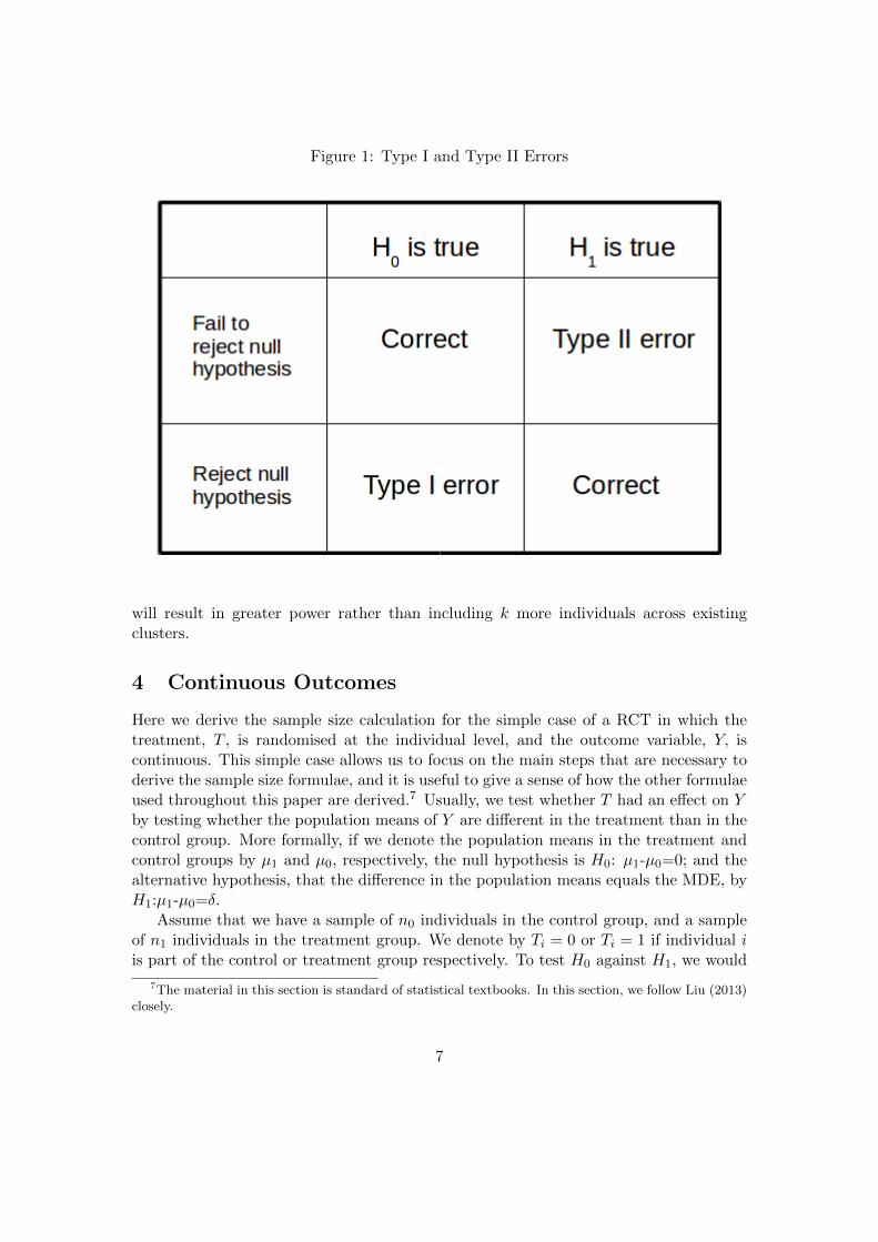
Figure 1: Type I and Type II Errors

will result in greater power rather than including k more individuals across existingclusters.

4 Continuous Outcomes

Here we derive the sample size calculation for the simple case of a RCT in which thetreatment, T , is randomised at the individual level, and the outcome variable, Y, iscontinuous. This simple case allows us to focus on the main steps that are necessary toderive the sample size formulae, and it is useful to give a sense of how the other formulaeused throughout this paper are derived.7 Usually, we test whether T had an effect on Yby testing whether the population means of Y are different in the treatment than in thecontrol group. More formally, if we denote the population means in the treatment andcontrol groups by µ1 and µ0, respectively, the null hypothesis is H0: µ1-µ0=0; and thealternative hypothesis, that the difference in the population means equals the MDE, byH1:µ1-µ0=δ.

Assume that we have a sample of n0 individuals in the control group, and a sampleof n1 individuals in the treatment group. We denote by Ti = 0 or Ti = 1 if individual iis part of the control or treatment group respectively. To test H0 against H1, we would

7The material in this section is standard of statistical textbooks. In this section, we follow Liu (2013)closely.

7

estimate the following OLS regression8:

Yi = α+ βTi + εi,

where Yi is the value of the outcome variable (say earnings in the case of APRENDE2)and εi is an error term with zero mean and variance σ2, which for the time being weassume it is known. The z-statistic associated with β is given by the OLS estimate of βdivided by its standard error, that is:

Z =Y1 − Y0

σ√

1n0

+ 1n1

,

where Y1 and Y0 are the sample averages of Yi for individuals in the treatment andcontrol group respectively, and σ is the standard deviation of Yi. If the null hypothesisis true, then µ1=µ0, and Z follows a Normal distribution with zero mean and varianceof one. Hence, the null hypothesis will be rejected at a significance level of α if Z≥zα/2 or Z≤ −zα/2, where the cumulative distribution function of the standard Normaldistribution evaluated at zα/2 is 1− α/2.

As mentioned above, power, denoted by 1−β, is the probability of rejecting the nullhypothesis when the alternative is correct, that is,

1− β = Pr(Z ≤ −zα/2 ∪ Z ≥ zα/2|H1) = Pr(Z ≤ −zα/2|H1) + Pr(Z ≥ zα/2|H1)

Because the alternative hypothesis is correct, µ1-µ0 is no longer zero, but δ. Hence, the

mean of Z is no longer zero but δ/(σ√

1n0

+ 1n1

). In this case, Pr(Z ≤ −zα/2|H1) is

approximately zero, and hence we have that9

1− β = Pr(Z ≥ zα/2|H1) = 1− Pr(Z < zα/2|H1)

By substracting the mean of Z under the alternative hypothesis from both sides of theinequality, we obtain

β = Pr(Z − δ

σ√

1n0

+ 1n1

< zα/2 −δ

σ√

1n0

+ 1n1

)

Because the left hand side of the inequality now follows a Normal distribution with zeromean and unit variance, it is the case that

z1−β = zα/2 −δ

σ√

1n0

+ 1n1

,

which implies that10

8We use a regression framework to keep the parallelism with forthcoming sections, but a t-test fortwo independent samples is equivalent

9See for instance Liu (2013). Note, however, that Liu (2013) defines zα/2 such that the cumulativedistribution function of the standard Normal distribution evaluated at zα/2 is α/2 instead of 1− α/2.

10Note that zβ = −z1−β .

8

zβ + zα/2 =δ

σ√

1n0

+ 1n1

In the case in which σ is unknown and is estimated using the standard deviation in thesample, then a t distribution with v = n0 + n1 − 2 degrees of freedom must be usedinstead of the Normal distribution. In this case, we have that

tβ + tα/2 =δ

σ√

1n0

+ 1n1

Solving for δ, we obtain the expression for the MDE that can be detected with 1 − βpower at significance level α:

δ = (tβ + tα/2)σ

√1

n0+

1

n1(1)

Alternatively, assuming that the sample size in the treatment and control groups arethe same, n0 = n1 = n∗, the expression for the sample size of each arm is given by:

n∗ = 2(tβ + tα/2)2σ

2

δ2(2)

It should be noted from equation 2 that for the results of a power calculation to bemeaningful, one must have accurate estimates of both the minimum detectable effectand the variance of outcomes, as both are key inputs.

Although subsequent equations will be more complicated, the derivation of these allfollows a similar approach to that above.

Finally for this section, we outline the case where variances are unequal, followingList et al. (2011). This case is uncommon in practice, as it is difficult a priori to considerhow the treatment will affect not just the mean of the outcomes, but the variance too.On example could be the provision of weather-linked insurance to farmers. Here onewould expect the variance of consumption to decline for the treated individuals. Totalsample size is defined as N = n0 + n1 and

δ = (tβ + tα/2)

√σ20n0

+σ21n1

After working through a series of equations ( see Appendix A for the full derivation),we derive a formula for N∗ and the optimal allocations of n0 and n1:

N∗ = (tβ + tα/2)2 1

δ2

(σ20π∗0

+σ21π∗1

), (3)

where π∗0 = σ0σ0+σ1

and π∗1 = σ1σ0+σ1

, and n∗0 = π∗0N∗ and n∗1 = π∗1N

∗. From this it canbe seen that the group with the larger variance is allocated a greater proportion of thesample.

9

4.1 Cluster Randomisation

In many cases, the outcome variable is measured at the individual level, but the randomi-sation takes place at the cluster level (school, village, firm)11. This may be driven byconcerns over spillovers within a cluster, whereby individual level randomisation wouldlead to control members outcomes being contaminated by those of treated individuals.In this case the sample size formula must be adjusted to reflect that observations fromindividuals of the same cluster are not independent, as they may share some unobservedcharacteristics.

The estimating equation will take the form of

Yij = α+ βTj + vj + εij , (4)

where i denotes individual, and j denotes the cluster. Tj is the treatment indicator, vjand εij are eror terms at the cluster and individual level. The variances of vj and εij aregiven by var(vj) = σ2c and var(εij) = σ2p, and σ2c + σ2p = σ2.

To carry out the sample size calculation in the presence of clustering, we require anadditional input; the intracluster correlation or ICC, denoted here as ρ:

ρ =σ2c

σ2c + σ2p

The ICC thus gives a measure of the proportion of the total variance accounted forby the between variance component. The intuition behind the ICC is that the larger thefraction of the total variance accounted for by the between cluster variance component(σ2c ), the more similar are outcomes within the cluster, and the less information is gainedfrom adding an extra individual within the cluster. Proceeding as in the simple caseabove, we derive the following equation12:

δ2 = (tα/2 + tβ)22

(mσ2c + σ2p

mk

), (5)

where there are k clusters per treatment arm and m individuals per cluster13. Using thedefinition of the ICC, and rearranging, we arrive at the formula for the total sample per

11We use the term individual to denote the level at which the observation is measured. In most cases itwill be people or households but it could also be firms (if the cluster is a town and the outcome variableis the profits of small businesses).

12 With clustering, and assuming equal variances for the two groups, the standard error of β takes theform: √(

σ2c

k+

σ2p

mk

)+

(σ2c

k+

σ2p

mk

)=

√2mσ2

c + σ2p

mk

13In the clustered case, the degrees of freedom in the t distribution are 2(k − 1).

10

treatment arm14:

n∗ = m∗k∗ = (tα/2 + tβ)22σ2

δ2(1 + (m− 1)ρ) (6)

Comparing equations 2 and 6, the key difference is the term (1 + (m − 1)ρ), whichis commonly referred to in the literature as either the design effect or the varianceinflation factor (VIF). This term is a consequence of the clustered treatment allocation,and will lead to larger required sample sizes. There is a slight additional difference,which means that one cannot simple calculate the individually randomised sample sizeand then multiply by the design effect. This is due to the fact that in the cluster-randomised case, the degrees of freedom for the t statistic are 2(k − 1) (not 2(n− 1) asin the individually randomised case). For this reason, the results presented in this paperwill differ slightly from those produced by software that does not adjust for degrees offreedom change.

In order to get a sense of the interplay between the ICC and the number per clus-ter, Table 1 presents required sample sizes for two different values of δ. We use theAPRENDE data here in order to get a standard deviation value, as well as reasonablevalues for δ. The actual ICC for this data is .042 - within the ranges of ICC valuespresented in Table 115. Consider first the upper left quadrant. The case where ICC=0represents individual level randomisation. As the ICC increases, so too does the samplesize. The extent of the increases depends also on m, the other key term in the VIF.One can see that for a ρ=.03, a rather small value for the ICC, and m=60, a clusterrandomised trial requires almost triple the sample size to that of an individual levelequivalent (7083 compared to 2557).

Another way to see this is to consider the upper right quadrant. At low levels of theintracluster correlation, there is a marked decline in the required number of clusters aswe increase m (the number of individuals per cluster). For ρ = .01, k drops from 279 to51, 18% of the initial value as we move move from left to right. As the ICC increases,this decline is much shallower. For ρ = .2 the right-hand value for k is 74% of the initialvalue. It should be clear from this table that its very important to get accurate measuresof key input parameters. Small differences in these values, such as moving from ρ = .01to .03, can have significant impacts on the required sample size, particularly when m islarge.

Finally, by comparing the upper and lower sections of Table 1, we see the impact ofthe size of the MDE - the larger is the value of δ, the smaller is the sample size requiredto detect a statistically significant effect.

14To operationalise this formula one can either solve for m as a function of k or solve for k as a functionof m. In the latter case (due to the fact that the degrees of freedom of the t distribution are a functionof the number of clusters (2(k− 1) in the absence of covariates)), it necessary to use an iterative processto ensure that the correct degrees of freedom (2(k∗ − 1)) are used to calculate the optimal number ofclusters, k*. This issue will be more pronounced when the number of clusters is small.

15In Appendix B we show how to compute the ICC using STATA.

11

4.1.1 Unequal Numbers of Clusters

It is useful to know what the equations look like for uneven allocations of both thenumber of clusters per treatment arm, k, and the number of individuals within theseclusters, m. This may be due to restrictions imposed on the size of one of the treatmentarms, for example because of logistical constraints. It should be noted that departingfrom an equal split for the two groups leads to a larger total required sample size, sothis should be done only when restrictions require so, or when this decreases the overallcost (for instance when control clusters are cheaper than treatment clusters - see section6.1). That said, total sample size only rises markedly for highly unbalanced allocations.The number of clusters in the treatment arm (k1) as a function of the number of clustersin the control arm (k0) is given by:

k1 =(tα/2 + tβ)2

(mσ2

c+σ2p

m

)δ2 − (tα/2 + tβ)2

(mσ2

c+σ2p

mk0

) (7)

This can also be written in terms of the design effect as:

k1 =(tα/2 + tβ)2σ2

(1+(m−1)ρ

m

)δ2 − (tα/2 + tβ)2σ2

(1+(m−1)ρ

mk0

) (8)

The formula for the number of individuals per treatment cluster (m1) as a function ofthe number of individuals per control cluster (m0) is given by:

m1 =(tα/2 + tβ)2

(σ2p

k

)δ2 − (tα/2 + tβ)2

(2σ2ck +

σ2p

m0k

) (9)

Rewriting in terms of ρ and σ yields:

m1 =(tα/2 + tβ)2σ2

((1−ρ)k

)δ2 − (tα/2 + tβ)2σ2

(1+(2m0−1)ρ

m0k

) (10)

4.2 The Role of Covariates

Although, due to randomisation, covariates are not used to partial out differences be-tween treatment and control, they can be very useful in reducing the residual varianceof the outcome variable, and subsequently leading to lower required sample sizes.

There are several different ways of representing the power calculation formula withcovariates, which will be presented for completeness, and due to the fact that in differentsituations, one may only have the required inputs suited to using a single formula.

The simplest or most intuitive version is as follows:

n∗ = m∗k∗ = (tα/2 + tβ)22σ2xδ2

(1 + (m− 1)ρx), (11)

12

where σ2x is the conditional variance (that is the residual variance once the covariates

have been controlled for), and ρx =σ2x,c

σ2x,c+σ

2x,p

the conditional ICC16. The form of equation

11 mirrors that of the unconditional representation in equation 6. If there is baselinedata, or data from a similar context with the relevant variables, it is straightforward toget estimates of these conditional parameters17. However, if this is not available, andestimates must be gleaned from the existing literature, it may be that these parametersare not directly obtainable. For this reason we present a different form of the conditionalpower calculation, which use different parameters. Bloom et al. (2007) present thefollowing formula:

n∗ = m∗k∗ = (tα/2 + tβ)22σ2

δ2(mρ(1−R2

c) + (1− ρ)(1−R2p)), (12)

where R2c is the proportion of the cluster level variance component explained by the

covariates, and R2p the individual level equivalent. This formulation is useful to see the

differing impact of covariates at different levels of aggregation i.e. if the covariates are atindividual or cluster level. For instance, an individual covariate can affect both R2

p andR2c , whilst a cluster level covariate can only increase R2

c . Equation 12 may be useful ifR2p and R2

c are reported in existing research, and the parameters in equation 11 are not.To reiterate, with a series of calculations, it is straightforward to move from equation 12to 11, using R2

c , R2p, σ

2 and ρ to obtain values for σ2x and ρx18.

Finally, Hedges and Rhoads (2010) present the formula for the inclusion of covariatesas:

n∗ = m∗k∗ = (tα/2 + tβ)22σ2

δ2[(1 + (m− 1)ρ)− (R2

p + (mR2c −R2

p)ρ)]

This equation may be useful for building intuition into the role of covariates, asthe first term in parentheses is the regular design effect, whilst the second shows howcovariates impact the overall variance inflation factor.

Table 2 presents how the inclusion of a covariate impacts the required sample sizesfor six different scenarios19 (m= 8, 20 and 100, ρ=.01 and .3). Values for the standarddeviation come from that of the earnings variable for 2002 in the APRENDE data. Asit is clear from equation 12, the larger either R2

p or R2c is, the smaller the sample size

per arm is. Note from equation 12 that the influence of R2p is larger when ρ is smaller.

For example, in Table 2, when ρ = 0.01, m = 100, and R2c=0, the sample size per

16In the case with covariates, the number of degrees of freedom of the t tistribution is 2(k − 1) − J ,where J is the number of covariates.

17Refer to Appendix B to see how to estimate these parameters.18Using the definition of ρx, we note that σ2(1− ρ)(1− R2

p) = σ2x,p = (1− ρx)σ2

x and σ2ρ(1− R2c) =

σ2x,c = ρxσ

2x. This allows us to write the R2 terms as functions of ρ, σ2, ρx and σ2

x: (1 − R2c) =

ρxσ2x

ρσ2

and (1−R2p) =

(1−ρx)σ2x

(1−ρ)σ2 . These expression are used in intermediate steps to move from equation 12 toequation 11.

19For this table we use a single individual level covariate. In the supplementary material we allow forindividual and cluster level covariates.

13

arm decreases from 1351 to 1043 (a 23% reduction) when R2p increases from 0 to 0.5.

However, the same increase in the R2p only translates into a decrease from 19342 to 19123

(a 1% reduction) when ρ = 0.3. In this sense, increasing R2p is similar to increasing the

number of individuals per cluster, which has little effect on power when ρ is high.As it is also clear from equation 12, the effect of R2

c is mediated by mρ, so thereduction in sample size achieved by increasing R2

c will be higher when both m and ρare large. Again, increasing R2

c is analogous to increase the number of clusters. This willhave a larger effect when ρ is large and when m is large (because a large m indirectlyimplies that the number of clusters is small, so we obtain a larger effect when we increasethem). This is also clear in Table 2: when ρ = 0.3, m = 100, and R2

p=0, the sample sizeper arm decreases from 19342 to 9940 (a 48% reduction) when R2

c increases from 0 to0.5. However, the same increase in the R2

p only translate in a decrease from 679 to 654(a 3.6% reduction) when ρ = 0.01 and m = 8.

A final point to note here is an issue raised by Bloom et al. (2007) regarding un-conditional versus conditional ICCs. As mentioned by the authors, one should not beconcerned with the possibility that an individual level covariate, by reducing the individ-ual level variance component by a larger extent than the cluster level component, maylead to a higher conditional ICC. What matters is that by reducing both components,individual level covariates increase precision and thus lower required sample sizes. Thisissue is not a concern with cluster level covariates, which can only impact σ2c , thus willalways lead to conditional variances and ICCs that are smaller than their unconditionalcounterparts.

4.2.1 Unequal Numbers of Clusters

As we presented in Section 4.1.1, we can write down the sample size equations whereeither k or m are unequal.

First, consider the expression for k1 as a function of k0 and m, written in the formpresented by Bloom et al. (2007)20:

k1 =(tα/2 + tβ)2σ2

(mρ(1−R2

c)+(1−ρ)(1−R2p)

m

)δ2 − (tα/2 + tβ)2σ2

(mρ(1−R2

c)+(1−ρ)(1−R2p)

mk0

) (13)

As before, we can also write an expression for m1 as a function of k and m021:

m1 =(tα/2 + tβ)2σ2

((1−ρ)(1−R2

p)

k

)δ2 − (tα/2 + tβ)2σ2

(2m0ρ(1−R2

c)+(1−ρ)(1−R2p)

m0k

) (14)

20We can also write an expression for k1 in the form of either equation 7, where we replace σc and σpwith σx,c and σx,p or equation 8, where we replace σ and ρ with σx and ρx.

21We can also write an expression for m0 in the form of either equation 9 or 10, replacing unconditionalparameters with their conditional versions.

14

4.3 Difference-in-Differences and Lagged Outcome as a Covariate

Where the researcher has not only data on the outcome variable subsequent to treatment,but also prior to treatment (baseline), it is possible to employ a difference-in-differencesapproach, as well as to include the baseline realisation of the outcome variable as acovariate, a special case of the approach above. Following Teerenstra et al. (2012) thedata generating process (which includes the panel component) follows:

Yijt = β0 + β1Tj + β2POSTt + β3(POSTt × Tj) + vj + vjt + εij + εijt,

where i indexes individuals, j clusters, and t time periods (t=0, the pre interventionperiod, or t=1, the post intervention period). POSTt takes the value 0 if t=0 and 1 ift=1, and Tj is the treatment indicator.

The error terms are structured as two cluster level components (vj and vjt) and twoindividual level components (εij and εijt), where vj and εij are time-invariant. Twoautocorrelation terms are required in this case, namely the individual autocorrelation ofthe outcome over time, ρp, and the analogous cluster level term, ρc:

ρp =σ2p

σ2p + σ2ptand ρc =

σ2cσ2c + σ2ct

,

where var(vj)=σ2c , var(vjt)=σ

2ct, var(εij)=σ

2p and var(εijt)=σ

2pt22. The ICC in this sita-

tion is expressed as23:

ρ =σ2c + σ2ct

σ2c + σ2ct + σ2p + σ2pt

Once these parameters are in hand, we can define the key parameter used in samplesize calculations, r, the fraction of the total variance composed of by the time invariantcomponents:

r =σ2c + σ2p/m

σ2c + σ2ct + σ2p/m+ σ2pt/m=

mρ

1 + (m− 1)ρρc +

1− ρ1 + (m− 1)ρ

ρp

The sample size formula for a difference-in-differences estimation can be written as

n∗ = m∗k∗ = 2(1− r)(tα/2 + tβ)22σ2

δ2(1 + (m− 1)ρ) (15)

and the sample size formula for an estimation using the baseline outcome variable as acovariate as:

n∗ = m∗k∗ = (1− r2)(tα/2 + tβ)22σ2

δ2(1 + (m− 1)ρ) (16)

In order to see the benefit of using the panel element, it is instructive to compareequations 15 and 16 with equation 6. The most important message is that the sample

22We note the abuse of notation in using t subscripts for the variance terms σ2ct and σ2

pt, as these termsare constant across the two time periods.

23Appendix C.5 details how to estimate these key panel data parameters.

15

size requirement is minimised by including the baseline level of the outcome variable asa covariate (note that 1 − r2 < 1 and that 1 − r2 < 2(1 − r)). Alternatively, given asample, the highest power is achieved by including the baseline value of the outcomevariable as covariate. Hence if baseline data on the outcome variable is available, oneshould always control for it as a covariate rather than doing difference-in-differences ora simple post-treatment comparison (McKenzie, 2012; Teerenstra et al., 2012).

Also, it is useful to see that the largest reduction on sample size requirements when weinclude the baseline value as covariate takes place when r is close to 1 (hence 1−r2 whichmultiplies the sample size formulae 16 is close to zero). Intuitively, by conditioning on thebaseline value of the outcome variable, we are netting out the time invariant componentof the variance (which is large when r is close to 1).

Note also that if r is close to zero, given a sample, there might be little differencein power between including the baseline value of the outcome as a covariate, and justpost-treatment differences. Hence, from the point of view of power, it might be betterto spend the resources devoted to collect the baseline on collecting a larger sample post-treatment or several post-treatment waves (see McKenzie (2012))24. Interestingly, interms of power, including the baseline value of the variable as covariate always dominatesover differences-in-differences. Moreover, baseline data is required for both estimators.Hence, there is little reason in terms of power to justify difference-in-differences

In Table 3, we report the sample size requirements for the three estimation strategiesfor various values of r, calibrating the calculations to the likely effect size and variance ofthe earnings for 2002 in the APRENDE data. The resulting sample sizes quantifies theintuition above - the higher the time invariant component of the variance, r, the greaterthe benefit of controlling for baseline differences via covariate or difference-in-differencesvis. a vis. single post-treatment difference. For low values of r, a difference-in-differencesstrategy is highly inefficient. The table also makes clear the dominance over the othertwo strategies of controlling for the baseline outcome as a covariate, for all values of r.

5 Binary Outcome Case

5.1 Individual Level Randomisation

Next, we move on to discussing the case where the outcome variable is binary, forinstance whether an individual is working or not or whether a student obtained a certaingrade level or not. There is a large literature that focusses on the binary outcome case,with several different approaches (for example Demidenko (2007), Moerbeek and Maas(2005)). Some papers deal with effect sizes measured in differences in log odds, otherswith differences in probability of success between treatment and controls. We followSchochet (2013) who measures the effect size in terms of differences in the probability ofsuccess. We believe that this is more intuitive for most economists, and that the required

24There might be other reasons to collect baseline data than gains in power. These vary from checkingwhether the sample is balanced in the outcome variables, to collect information that allow to stratifythe sample, and to have the basis for heterogeneity analysis (see McKenzie (2012)).

16

inputs might be more easily accessible from published studies25. One difference betweenthe continuous and the binary outcome case is that in the latter, we do not need thevariance. Binary outcomes follow a Bernoulli distribution, so knowing p, the probabilityof success, also yields the variance; p(1− p).

Using a logistic model, we can write the probability of success for individual i as:

pi = Prob(yi = 1|Ti) =eβ0+β1Ti

1 + eβ0+β1Ti,

where yi is binary (takes value 1 in case of success and 0 in case of failure) and as before,Ti denotes treatment status. The effect size, δ can thus be written as p(yi = 1|Ti =1) − p(yi = 1|Ti = 0) or (p1 − p0), where the subscripts denote treatment and controlstatus respectively.

Following an analogous procedure as in the continuous case, we arrive at a samplesize equation for the binary case (Donner and Klar, 2010):

N∗ =

(p1(1− p1)

π+p0(1− p0)

1− π

)(zβ + zα/2)

2

(p1 − p0)2, (17)

where π is the proportion of the sample that is treated26, n∗1 = πN∗ and n∗0 = (1−π)N∗.Note that equation 17 is equivalent to equation 3, where σ20 and σ21 are replaced withtheir equivalents in the binary case, p0(1−p0) and p1(1−p1). In general, these varianceswill be different, so as we saw in equation 3, the optimal treatment-control split willdiffer from .5. The optimal allocation to treatment status, π∗ can be written as:

π∗ =

√p1(1−p1)p0(1−p0)

1 +√

p1(1−p1)p0(1−p0)

(18)

Hence, in the binary outcome case, the optimal split would only equal .5 in thespecial case where p0=1− p1 for example p0=.4 and p1=.6. In that case of an even splitbetween treatment and control status (π = .5), we can write n∗ as

n∗ = (p1(1− p1) + p0(1− p0))(zβ + zα/2)

2

δ2(19)

5.2 Cluster Level Randomisation

Having considered the individual level treatment case, we now move to cluster ran-domised treatment, still following Schochet (2013), as we do for the rest of section 5.

25An advantage of the approach we follow is that the impact parameter does not depend on whethercovariates are included or not. This is not the case when impact is measured in log odds. See Schochet(2013) for a detailed discussion of this.

26If the null hypothesis of zero impact is tested using a Pearson’s chi-square test, and n∗1 = n∗0, then

n∗ =(zα/2

√2p(1−p)+zβ

√p1(1−p1)+p0(1−p0))2

(p0−p1)2where p = p1+p0

2, (see Fleiss et al. (2003) equation 4.14, as

well as equation 4.19 for different sample sizes in treatment and control).

17

For the cluster randomised case, a Generalised Estimating Equation (GEE) approach isfollowed, where the clustering is accounted for in the variance-covariance matrix, usingthe ICC, ρ. As before we can write the probability of success for individual i in clusterj as

pij = Prob(yij = 1|Tj) =eβ0+β1Tj

1 + eβ0+β1Tj,

For cluster j, the m×m variance covariance matrix Vj is written as

Vj = A1/2j R(ρ)A

1/2j , (20)

where Aj is a diagonal matrix with diagonal elements pij(1−pij) and R(ρ) is a correlationmatrix with diagonal elements taking the value of 1, and off-diagonals the value of ρ.Hence cov(yij , ykm) = ρ when j = m and =0 when j 6= m. Note the lack of a j subscripton R(ρ) - it is taken as common across clusters, as in the Generalised Least Squares(GLS) approach for a continuous outcome. This means that we no longer specify arandom effect for each cluster, and allows us to get closed form solutions for the samplesize equations27.

The sample size equation for the binary outcome case with cluster randomisationcan be written as:

N∗ =

(p1(1− p1)

π+p0(1− p0)

1− π

)(zα/2 + zβ)2

δ2(1 + (m− 1)ρ), (21)

where π is the fraction of clusters randomised to receive treatment, n∗1 = mk∗1 = πN∗

and n∗0 = mk∗0 = (1−π)N∗. As above, if the treatment is evenly allocated, we can writethis as

n∗ = mk∗ = (p1(1− p1) + p0(1− p0))(zβ + zα/2)

2

δ2(1 + (m− 1)ρ) (22)

As before, the sample size equation for the binary outcome mirrors that of the con-tinuous outcome, with the design effect being the only difference between the individualand cluster randomised sample size equations.

Table 4 presents sample size requirements for three different levels of success prob-ability for the control groups, p0; 0.1, 0.3 and 0.5. The first thing to notice is that thecloser p0 is to .5, the larger the is sample size required. This is because for a binaryvariable, variance is largest at p=0.5. For example, for m=30 and ρ=.03, the samplesize for p0=0.5 is double that of p0=.1. As in the continuous case, we see that higherICCs and larger cluster sizes, m, lead to larger required total samples. This is due tothe design effect.

27Results from simulations we ran utilising the GEE approach yielded very similar results to thoseusing a linear probability model with random effects. Schochet (2009) finds similar results using GEEand random effects logit models too.

18

5.2.1 Unequal Numbers of Clusters

It might be useful to have a formula for k1 as a function of m and k0, that will providepower of (1− β) for the given m and k0:

k1 =

p1(1−p1)m (zα/2 + zβ)2(1 + (m− 1)ρ)

δ −(p0(1−p0)mk0

)(zα/2 + zβ)2(1 + (m− 1)ρ)

(23)

5.3 The Role of Covariates

In this section, we consider the case of individual treatment allocation where one has asingle covariate, Xi, that is discrete, but not necessarily binary. In the case where theXi is continuous, one can discretise the variable. Here, we write pi as

pi = Prob(yi = 1|Ti, Xi) =eβ0+β1Ti+β2Xi

1 + eβ0+β1Ti+β2Xi

Where covariates are included, we need several extra inputs into the sample size equa-tion, relating to the distribution of the covariates, and how success probabilities changeaccording to the covariate values.

First, assume that Xi can take any of the following Q values, {x1, ......, xQ}. Defineθq = Prob(Xi = xq) for q ∈ {1, ....., Q} , with (0 < θq < 1) and

∑q θq = 1. Next

we need to specify how success probabilities change across the values of Xi. Definep0q = Prob(Yi = 1|Ti = 0, Xi = xq) and p1q = Prob(Yi = 1|Ti = 1, Xi = xq). Then wecan define an effect size for a specific value of q, δq = p1q−p0q, and an overall effect size,δ =

∑q θqδq. Schochet (2013) notes that covariate inclusion will improve efficiency if at

least two of the p0q or p1q probabilities differ across covariate values.With these inputs at hand, we can now write the sample size equation as:

N∗ = (gM−1g′)(zβ + zα/2)

2

δ2, (24)

where

M =

m1 m2 m3

m2 m2 m4

m3 m4 m5

,

19

m1 =∑q

{πθqp1q(1− p1q) + (1− π)θqp0q(1− p0q)}

m2 =∑q

{πθqp1q(1− p1q)}

m3 =∑q

xq{πθqp1q(1− p1q) + (1− π)θqp0q(1− p0q)}

m4 =∑q

xq{πθqp1q(1− p1q)}

m5 =∑q

x2q{πθqp1q(1− p1q) + (1− π)θqp0q(1− p0q)}

and g is a 1× 3 gradient vector with elements:

g[1, 1] =∑q

θq[p1q(1− p1q)− p0q(1− p0q)]

g[1, 2] =∑q

θq[p1q(1− p1q)]

g[1, 3] =∑q

xqθq[p1q(1− p1q)− p0q(1− p0q)]

In the Appendix section D we provide a purposefully designed STATA programme tocarry out this computation for 5 different values of covariates28.

5.3.1 Cluster Level Randomisation

Finally we consider a cluster randomised treatment in the presence of a single, discretecluster level covariate. Candidates for this could be a discrete cluster characteristic or acontinuous variable, such cluster means of the outcome variable at baseline, which arethen discretised. We write the probability of success here as

pij = Prob(yij = 1|Tj , Xj) =eβ0+β1Tj+β2Xj

1 + eβ0+β1Tj+β2Xj,

The variance-covariance matrix in this scenario is very similar to that without a covariate(see equation 20) with the exception of the use of the conditional ICC, ρx, not the rawICC (ρ) in the correlation matrix. The sample size calculation for this section can beexpressed as

N∗ = 2m∗k∗ = (gM−1g′)(zβ + zα/2)

2

δ2(1 + (m− 1)ρx), (25)

28As supplementary material we supply STATA programmes for 2, 3, 4 and 5 possible values of thecovariate. Schochet (2013) provides a set of SAS programmes for sample size calculations for binaryoutcomes.

20

where g and M are defined as above, and ρx is the conditional ICC, as we saw inthe continuous outcome case with cluster randomisation and covariates. Note that theinclusion of a cluster level covariate can lead to precision gains through decreasing thetotal residual variance, as well as by decreasing the conditional ICC. Schochet (2013)suggests that the latter will have more impact on lowering the required sample size.

Table 5 presents the number of clusters required in the binary outcome case for twovalues of ρ; 0.05 and 0.1, and a binary covariate. What we see here is that the greateris the difference between p00 and p01 (the difference in control group success rates forthe two values of the covariate), the greater is the sample size reduction due to theinclusion of the covariate. The number of clusters required (for m=60, ρ=.05, p0=.5,and a constant effect size of .1 across covariate levels) is 51 in the absence of a covariate(bottom right section of Table 4). In Table 5, this number falls to 49 when p00=.4 andp01=.6, and falls markedly to 32 when p00=.2 and p01=.8. In this example, the spreadin impact values across the values of X has a more noticeable effect when the spread incontrol group success rates across X values is larger.

6 Extensions

6.1 Optimal Sample Allocation Under Cost Constraints

In the previous sections, we have described how to compute the sample size that willallow us to reach a desired level of power. However, we did not take into account anycost considerations, which are usually very relevant for researchers. Researchers have anumber of degrees of freedom when designing the sample of a study: ratio of the samplesize in the treatment versus control group, number of clusters vs. number of individualswithin a cluster, etc. Hence, it makes sense to choose the options that minimise costswithout decreasing power29.

In our previous examples, we have assumed the number of treatment and controlunits (clusters and/or individuals) to be the same. This is a common strategy used byresearchers because it maximises the power of the study given a total sample (this is thecase for continuous outcomes. As discussed in section 5.1, for the binary outcome case,an even treatment-control split is unlikely to optimal in general). If the costs of thestudy depend solely on the total sample, then this approach will also maximise powergiven a total cost30. Hence, the approach will also minimise costs for a given level ofpower.

However, it is easy to think of cases where the costs do not depend solely on thetotal sample, but also of other parameters. For instance, if the research budget includesthe cost of running the intervention then treatment units will be more expensive than

29Here, we do not study how to minimise costs as function of the autocorrelation of the outcomevariable. For low autocorrelated outcomes, costs might be minimised subject to a given level of powerby not having baseline, but multiple post-treatment measures (McKenzie, 2012).

30This implicitly assumes that the variance of the outcome variable in treatment and control groups isthe same. In situations when this is not true, power is maximised if the group with the higher varianceis larger (for example see equation 3).

21

the control ones. In these situations, we can maximise power (given an overall cost)by allocating a larger sample to the control group than the equal split. To understandthe intuition, starting from the equal split, allocating units from treatment to controlwill result in a overall cost reduction but also loss of power because of the imbalance.However, the latter could be more than offset if we use the part of the cost reductionto boost total sample size. But of course, this will have a limit. As the loss of powerincreases more than linearly with the imbalance, the loss of power might not be offset ifthe sample is already highly unbalanced.

To allow the user to operationalise the above, below we provide the formulae thatallows us to compute C∗, the minimum cost that allow us to detect a given MDE, δ. Thiswill be of use for the researcher that has a clear view on the MDE of the interventionthat she is testing, and wants to find out the minimum cost that will allow her to detectit in order to submit a competitive bid. We also provide formulae for δ∗ which is thefeasible MDE given a total cost C. This will be of more use to the researcher that hasa binding cost constraint and is figuring out how effective her intervention must be inorder to detect its effect under the cost constraint. The specific formulae depends onthe specific structure of the cost function. We specify a different one on each of thesubsections below31.

6.1.1 Individual Level Randomisation

There are many different variations of cost functions we may specify. Here we present afew alternatives. First consider the situation where treatment allocation is individuallyallocated and the cost function is given by

C = c0n0 + c1n1

Once we have specified the cost function, we then solve a constrained optimisationproblem, minimising the MDE subject to the cost function. This yields a solution interms of n0, n1 and the cost function parameters32:

n1n0

=

√c0c1

(26)

Hence, the more expensive the treatment units are, the smaller the treatment groupwould be compared to the control. Using the cost function, we can write n0 and n1 asfunctions of the cost parameters:

n∗0 =C

c0 +√c0c1

and n∗1 =C

c1 +√c0c1

(27)

31In what follows we provide formulae for optimal allocations for continuous outcomes. One can followa similar approach to the one outlined below to derive the equivalent formulae for binary outcome cases.

32The equivalent formula for the discrete case is: n1n0

=√

c0c1

p1(1−p1)p0(1−p0)

.

22

The relations in equation 27 would be combined with equation 1 to obtain the smallestMDE achievable in order to obtain a power of 1− β given the budget constraint C:

δ∗ = (tβ + tα/2)σ

√1

n∗0+

1

n∗1, (28)

which leads to a formula for δ∗ as a function of the cost parameters:

δ∗ = (tβ + tα/2)σ√C

(√c0 +

√c1) (29)

This formulation is useful in order to assess whether or not to conduct a trial at a givenbudget, C. For instance, if the budget for the trial, C, were very small, this wouldlimit the number of individuals in the trial, and would thus require a very large effectsize in order to achieve a power of 1 − β. If this effect size is unrealistic, the RCT isunder-powered with the given budget. Alternatively we can derive an expression for theminimum total cost, C∗, required in order to achieve a power of 1−β with a given valueof δ. In order to do so, we use the relations in equations 27 and 28:

C∗ = (tβ + tα/2)2σ

2

δ2(√c0 +

√c1)

2 (30)

In order to get a sense of the value of the constrained optimisation methods outlinedin this section, Table 6 presents the cost savings from using the optimal sample alloca-tions (which account for different unit costs, c0 and c1) compared to the non-optimisedallocations (i.e. where n0=n1, irrespective of the cost differences). For example, wherec0 = 50 and c1 = 200, we see that n∗0 = 2n∗1 (which comes directly from equation 26),resulting in a 10% cost saving. The greater the difference in unit costs, the greater theresulting difference in optimal sample allocation, and thus the greater the cost savingsfrom using optimal sample allocations.

6.1.2 Cluster Level Randomisation with Heterogenous Cluster Costs

Moving on to the cluster randomisation case, we follow the same method as above, firstspecifying a cost function and then minimising the MDE subject to this cost function.For instance, if the treatment is the provision of a cluster level service or amenity (aclean well or improved sanitation amenities at the village level), then the only differencebetween the costs of treatment and control areas will be the fixed cost of this serviceprovision, yielding a cost function of the form:

C = f0k0 + f1k1,

where f0 = f ′0 + vm and f1 = f ′1 + vm. Here, the cluster size is fixed at a certainm33, thus we do not consider this dimension of the sample when optimising. Solving a

33For example, where the cluster is a school, and the outcome variable is the result of a test taken byall pupils in the school, m.

23

constrained optimisation problem as before (where the objective function is the squareof the MDE) gives us the following solution34:

k1k0

=

√f0f1

As before, we use the cost function to write the optimal values of k1 and k0 as functionsof the cost parameters:

k∗0 =C

f0 +√f0f1

and k∗1 =C

f1 +√f0f1

(31)

The remaining step in this constrained optimisation problem is to use equation 8with equation 31 to compute the effect size as a function of the optimal values of k0 andk1, which will yield the minimum effect size that will need to be found in order to obtaina power of 1− β, given the budget constraint, C35:

δ∗ = (tα/2 + tβ)

√σ2(

1 + (m− 1)ρ

mk∗0+

1 + (m− 1)ρ

mk∗1

), (32)

which can be written in terms of the cost function parameters as:

δ∗ = (tα/2 + tβ)

√σ2(1 + (m− 1)ρ)

(f0 +

√f0f1

mC+f1 +

√f0f1

mC

)(33)

We can also derive an expression for the minimum total cost, C∗, required in orderto achieve a power of 1− β with a given value of δ. To do so, we combine equations 31and 32 to arrive at:

C∗ = (tα/2 + tβ)2σ2

δ2(1 + (m− 1)ρ)

m

(√f0 +

√f1

)2(34)

6.1.3 Cluster Level Randomisation with Heterogenous Individual Costs

Were the treatment to have an individual level component, such as a vaccination pro-gramme or a job training programme, then the variable costs may be of more relevance.This may give rise to a cost function such as:

C = 2fk + v0m0k + v1m1k,

where k is fixed and f represents the fixed cost of data collection at the cluster. Theconstrained optimisation problem yields the following ratio:

34In this section, we ignore that the degrees of freedom of the t-distribution are a function of thenumber of clusters, k. This will normally have a minimal effect on the sample size, unless the numberof clusters is very small.

35We provide the formulae for the case without covariates. One can replace σ2 with σ2x and ρ with ρx

to adapt the formulae to the case with covariates.

24

m1

m0=

√v0v1,

which we can combine with the cost function in order to get the following expressionsfor optimal values of m0 and m1:

m∗0 =C − 2fk

k(v0 +√v0v1)

and m∗1 =C − 2fk

k(v1 +√v0v1)

(35)

As we saw in section 6.1.2, the final step now is to use equation 10 with equation 35 tocompute the effect size as a function of these optimal values of m0 and m1, which willyield the minimum detectable effect size required to achieve a power of 1− β, given thebudget constraint, C:

δ∗ = (tα/2 + tβ)

√σ2(

1 + (m∗0 − 1)ρ

m∗0k+

1 + (m∗1 − 1)ρ

m∗1k

), (36)

which we can write in terms of the cost function parameters as:

δ∗ = (tα/2 + tβ)

√σ2(

2ρ

k+

(1− ρ)(√v0 +

√v1)2

C − 2fk

), (37)

Finally, we can derive an expression for the minimum total cost, C∗, required in orderto achieve a power of 1− β with a given value of δ. To do so, we combine equations 36and 35:

C∗ = 2fk +(tα/2 + tβ)2σ2(1− ρ)(

√v0 +

√v1)

2

δ2 − (tα/2 + tβ)2σ2(2ρk )(38)

6.1.4 Cluster Level Randomisation with Homogenous Individual and Clus-ter Costs

We now consider a cost function with homogenous individual and cluster costs. The aimhere is to achieve an optimal allocation of the total sample into number of clusters, k,and cluster sizes,m. The cost function thus takes the form

C = k(f + vm),

where f is the fixed cost per cluster, and v the variable cost, per individual. Minimisingthe square of the MDE (as given in equation 5) subject to this cost constraint yieldsoptimal values for m:

m∗ =

√f

v

σ2pσ2c

(39)

25

Using this formula and the form of the cost function we derive an expression for theoptimal k:

k∗ =C

f + v

√fv

σ2p

σ2c

(40)

As Liu (2013) notes, it my be instructive to use the definition of the ICC to rewriteequations 39 and 40 as:

m∗ =

√f

v

1− ρρ

and k∗ =C

f + v√

fv1−ρρ

(41)

Here we see that the larger is the ICC, the smaller the optimal m. This is due to the factthat when the ICC is high, outcomes within clusters are highly correlated, and increasingthe number within the cluster, m, adds little in precision gains. Resources are betterspent by increasing the number of clusters, k.

With the optimal values of m and k in hand, we can compute the minimum effectsize in order to achieve power of 1− β, given the budget constraint, C:

δ∗ = (tα/2 + tβ)

√2σ2

(1 + (m∗ − 1)ρ

m∗k∗

)(42)

To complete this section, we derive an expression for the minimum total cost, C∗,required in order to achieve a power of 1− β with a given value of δ. In order to do so,we combine equations 42 and 41:

C∗ =2σ2

δ2(tα/2 + tβ)2

[f + v

√f

v

1− ρρ

]1 + (√

fv1−ρρ − 1)ρ√

fv1−ρρ

(43)

6.1.5 More Complex Cost Functions

The researcher might face more complex design features that the ones discussed above,and the optimal allocation might require different number of treatment and controlclusters, and/or different number of individuals sampled across treatment and controlclusters. In such complex cases, it may not be possible to find an analytical solutionto the constrained optimisation problem. For these situations, it is useful to generaliseequation 5 and express the MDE as:

δ2 = (tα/2 + tβ)2

(σ2ck0

+σ2pm0k0

+σ2ck1

+σ2pm1k1

).

In general, the optimal allocation of k0, k1, m0, andm1 will be obtained by minimising(σ2ck0

+σ2p

m0k0+ σ2

ck1

+σ2p

m1k1

)subject to a cost constraint36. For specific parameter values,

36Note that minimising the MDE is equivalent to maximizing power. Note also that the other com-ponents of the MDE formulae are fixed with the sample

26

this minimisation can be done using numerical optimisation software. An example ofthis can be found in Appendix E, where we use STATA’s optimize function (which isrun from MATA) to solve for the constrained optimisation problem under the complexcost function C = k0(f0 + v0m0) + k1(f1 + v1m1)

37.There are some simplified cases in which one can also combine some of the previ-

ous results with a grid search on one of the unknown parameters to find the optimalsolution using a simple spreadsheet. For instance, consider the case in which treat-ment and control cluster fixed costs are different but m is not given, so an optimal mmust be found. This would be as the case of subsection 6.1.2 but with unknown m.Hence, using that f0=f

′0+vm and that f1=f

′1+vm, different values of f0 and f1 can be

computed for each possible m. These will lead to different values of k0 and k1 usingequation 31. The optimal combination of m, k0 and k1 will be the one that minimises(σ2ck0

+σ2p

mk0+ σ2

ck1

+σ2p

mk1

).

Another simplified case which is likely to be of interest is when the treatment andcontrol variable cost per observation are different, but the fixed cost per cluster are thesame. This is the case of section 6.1.3 but where k is not given, and an optimal valuefor it must be found. Again, a grid search for different values of k can be used to findthe optimal combination of k,m0,m1. For each different value of k, the correspondingvalues of m0 and m1 can be computed using equations 35. The optimal combination of

k, m0 and m1 will be the one that minimises(σ2ck +

σ2p

m0k+ σ2

ck +

σ2p

m1k

).

In practice, the cost function might not be as simple as the one used above. Forinstance, costs could increase discontinuously in the number of individuals per cluster ifinterviewers must spend an extra night, or a new vehicle must be purchased to be ableto cover more than a certain amount of clusters in a given time period. However, theexercise of computing the cost for each combination of clusters and number of individualsper cluster should be feasible. This information can be embedded within an isopowercurve, which yields the different combinations of clusters (k) and individuals per cluster(m) that provide the same level of power38. The cost information, together with theisopower curve, will allow the researcher to choose the combination that minimises cost.There may be cases where the data collection is commissioned to a survey firm thatis not willing to share the cost function. In these circumstances, the researcher canprovide possible combinations of number of clusters and number of individuals (fromthe isopower curve), and the survey firm can choose the one that minimises its costs.

37For chosen parameter values, and for the specific initial inputs of the unknown values (in this casefor m1, k0 and k1), the optimize programme yielded a solution within five iterations. However, given theshape of the objective function, the programme was very sensitive to the choice of initial values for theunknowns, in many cases never converging to a solution. As with most numerical optimisation routines,the user is advised to try with different starting values.

38using formulae such as equations (8), (10), (13), (14) or (23) depending on the case

27

6.2 Simulation

A researcher might need to compute the required sample size for an experiment whosefeatures do not conform to the ones indicated in previous sections. The possibilities ofvariation are endless. They include experiments in which the number individuals percluster varies across clusters, experiments with more than two treatment arms, or usingdata from more than two time periods, to say a few. In situations where some featuresof the experimental design vary significantly with respect to the canonical cases givenabove, simulation methods can be very useful to estimate the power of a given design,and correspondingly adjust the sample of the design to achieve the desired level of power.

To understand the logic of the simulation approach, it is useful to remember thedefinition of power: the probability that the intervention is found to have an effect onoutcomes when that effect is true. In a hypothetical scenario in which the researcherhappened to have 1,000 samples as the ones of her study, and if she could be certainthat “the effect is true” in all these samples, then she could estimate such probability(power) by simply counting in how many of these samples she “finds” the effect (the nullhypothesis of zero effect is rejected), and dividing it by 1,000.

The simulation approach simply operationalises the above by providing the researcherwith 1,000 (or more) computer-generated samples, hopefully similar to the one of herstudy (or at least, obtained under the assumptions that that the researcher is planningthe study). Because these are computer-generated samples, the researcher can obtainthese samples imposing the constraint that the effect is true (and in particular, it willdraw the samples assuming that the effect of the intervention is the same as the effectsize, δ, for which she wants to estimate the power).

In general, the steps required to estimate the power of a given design through simu-lation are as follow (see Appendix C for an example)39:

Step 1 : define the number of simulations that will be used to estimate the power ofthe design, say S; as well as the significance level for the tests.

Step 2 : define a model that will be used to draw computer-generated samples “asthose in the study”. This model will have a non-stochastic part (sample size, numberof clusters, distribution of the sample across clusters, number of time periods, ICC,autocorrelation terms, mean and standard deviation of the outcome variable, effect size,etc) and a stochastic part (error term)40. An example of such model could be, forinstance, equation 4 but for specific values for the effect size, standard deviation andICC (in Appendix C.6 these are set as δ = 4, σ = 10 and ρ = .3 ).

Step 3 : using computer routines for pseudo-random numbers, obtain a draw of theerror term (or composite of error terms) for each individual in the sample. It is crucialthat the error term is drawn taking into account the stochastic structure of our exper-iment (the correlation of draws amongst different individuals and time periods throughthe ICC or similar parameters). To draw samples from the error terms, a distribution

39Feiveson (2002) provide insightful examples for Poisson regression, Cox regression, and the rank-sumtest.

40If a pilot dataset is available, an alternative approach is to bootstrap from this data(see Kleinmanand Huang (2014)).

28

will need to be assumed. Although assuming Normality is common, the approach allowsto assume other distributions that might be more appropriate for the specific experiment.

Step 4 : using the model and parameter values indicated in Step 2, and the sampleof the error term (or composite of error terms) generated in Step 3, obtain the valuesof the outcome variable for the sample. Once this is done, the draws of the error termgenerated in Step 3 can be discarded.

Step 5 : using the data on outcomes generated in Step 4, and the model of Step 2,test the null hypothesis of interest (usually, that the intervention has no effect41). Keepa record of whether the null hypothesis has been rejected or not.

Step 6 : Repeat Steps 3 to 5 for S timesStep 7 : the estimated power is the number of times that the null hypothesis was

rejected in Step 5 divided by S.Although using simulation methods to estimate power has a long tradition in statis-

tics, the approach is not so commonly used in practice (Arnold et al. 2011)42. Wesuspect that Step 3 is the most challenging for the applied researchers. In Appendix C,we provide several hints, which could be of some help.

6.3 Adjusting Sample Size Calculations for Multiplicity

A common problem with experiments (and more generally in empirical work) is that,more than one null hypothesis is usually tested. For instance, it is common to test theeffect of the intervention on more than one outcome variable. This creates a problembecause the number of rejected null hypothesis (the number outcome variables for whichan effect is found) will increase (independently of whether they are true or not) withthe number of null hypotheses (outcome variables) tested if the significance level is keptfixed with the number of hypotheses.

For instance, consider that we are testing the effect of an intervention on threedifferent outcome variables, and that we use an α equal to 0.05 for each test. If we assumethat the three outcome variables are independent, then probability that we do not rejectany of the three when the three null hypotheses are all true is (1 − 0.05)3. Hence, theprobability that we reject at least one of them if the three are true is 1−(1−0.05)3 = 0.14.Why is this a problem? Assume that the intervention will be declared successful it isfound that it improves at least one of the outcomes. The numbers above implies thatthe intervention will be declared successful with a probability of 0.14 (larger than thenormal significance level of 0.05) even if it has no real effect on any of the three outcomevariables.

The problem of multiplicity of outcome variables is recognised by regulatory agenciesthat approve medicines (Food and Drug Administration (1998) and European MedicinesAgency (2002)) and has recently become more common also in applied work in economics

41We are assuming that the test for the null hypothesis has the correct size. Otherwise see Lloyd(2005)

42See Hooper (2013), Kontopantelis et al. (Forthcoming), and Kumagai et al. (2014) for some recentimplementations of the simulation approach to estimate power.

29

(Anderson (2008), Carneiro and Ginja (2014)43). The standard solution requires per-forming each individual hypothesis test under an α smaller than the usual 0.05 (Ludbrook1998, Romano and Wolf 2005) so that the probability that at least one null hypothesesis rejected when all null hypotheses are true ends up being 0.0544. Hence, when doingthe sample size calculations, the researcher should also use a smaller α than 0.05, whichwill increase the sample size requirements.

When the outcome variables are independent, the probability that at least one nullhypothesis is rejected when all are true, usually called the Family Wise Error Rate(FWER) is 1− (1− α)h, where α is the level of significance of the individual tests andh is the number of null hypothesis that are tested (i.e. number of outcome variables).Hence, if our study needs a FWER =0.05, then the significance level for each individualtest is given by 1− (1− 0.05)(1/h), which would be 0.0169 in our example of h = 345.

In most experiments, the outcome variables will not be independent. Taking intoaccount this dependency will yield higher values of α, and consequently smaller samplesize requirements. If one was willing to assume the degree of dependency amongst thedifferent outcome variables, then a time consuming but feasible approach to computethe required power is to use the simulation methods previously described combined witha method for Step 5 (testing the null hypothesis) that takes into account the multipletests carried out and the dependence in the data (such as Romano and Wolf (2005)or Westfall and Young (1993)). If this was not available, a rule of thumb is to use

α = 1− (1− 0.05)(1/√h), a correction which was popularised by John W. Tukey(Braun,

1994). This will result in an α larger than when independence is assumed, and hencesmaller sample size requirements.

7 Conclusion

In this paper, we have reviewed the methods to provide sample size calculations for stud-ies that go beyond the simple comparisons of treatment and control averages. Extensionshave included how to maximise power given a cost constraint, adjusting the sample sizecalculations when multiple outcomes are being tested, and the use of simulation exercisesto estimate the power of more complex designs not covered so far.

Researchers will need to make more assumptions when taking advantage of thesemore complex methods that we provide here than in simpler ones. However, we believethat the increasing availability of publicly available datasets means that researchers are ina relatively good position to make credible assumptions about the required parameters.Researchers could also help other researchers by reporting basic parameters such asintra cluster correlations, individual and cluster level correlations, and R-squares intheir papers. Journal editors could help to speed up the process by coordinating on

43There is less consensus on whether correcting for multiplicity is necessary when testing multipletreatments (see Wason et al. (2014)).

44An alternative way to analyse the data is to test jointly (through an F-test) the null hypotheses thatthe intervention does not have an impact on any of the outcome variables considered.

45A common simplification is to use the Bonferroni correction, which would be 0.05/h

30

certain reporting, rules as it has happened in Medicine (Schulz et al., 2010).Our experience is that researchers more often than not, tend to go for an equal split

of sample size between treatment and control, before thinking how an unequal splitcould decrease the costs (or provide more power at the same cost). The formulae andother information that we have provided here might enable researchers to improve onthis practice.

Another issue in which we expect further development in the future is to consideradjustments in the sample size calculations when the RCT considers multiple outcomes.It is starting to make its way on empirical work to adjust the p-values when multiplehypotheses are being tested. Hence, it is only a question of time that this adjustment isnot only done ex-post once the data is collected, but considered ex-ante when the studyis being designed and the sample planned.

References

Anderson, M. L. (2008): “Multiple Inference and Gender Differences in the Effects ofEarly Intervention: A Reevaluation of the Abecedarian, Perry Preschool, and EarlyTraining Projects,” Journal of the American Statistical Association, 103, 1481–1495.

Bloom, H. S., L. Richburg-Hayes, and A. R. Black (2007): “Using Covariatesto Improve Precision for Studies That Randomize Schools to Evaluate EducationalInterventions,” Educational Evaluation and Policy Analysis, 29, 30–59.

Blundell, R. and M. Costa Dias (2009): “Alternative Approaches to Evaluation inEmpirical Microeconomics,” Journal of Human Resources, 44, 565–640.

Braun, H. I. e. (1994): The collected works of John W Tukey Vol. VIII. Multiplecomparisons : 1948-1983, New York: Chapman & Hall.

Burtless, G. (1995): “The Case for Randomized Field Trials in Economic and PolicyResearch,” Journal of Economic Perspectives, 9, 63–84.

Carneiro, P. and R. Ginja (2014): “Long-Term Impacts of Compensatory Preschoolon Health and Behavior: Evidence from Head Start,” American Economic Journal:Economic Policy, 6, 135–73.

Demidenko, E. (2007): “Sample size determination for logistic regression revisited,”Statistics in Medicine, 26, 3385–3397.

Donner, A. and N. Klar (2010): Design and Analysis of Cluster RandomizationTrials in Health Research, Chichester: Wiley, 1st ed.

Duflo, E. (2006): “Field Experiments in Development Economics,” Tech. rep., MIT.

Duflo, E., R. Glennerster, and M. Kremer (2007): “Chapter 61 Using Random-ization in Development Economics Research: A Toolkit,” Elsevier, vol. 4 of Handbookof Development Economics, 3895 – 3962.

31

European Medicines Agency (2002): “Points to Consider on Multiplicity Issues inClinical Trials,” Tech. rep.

Feiveson, A. (2002): “Power by simulation,” Stata Journal, 2, 107–124.

Fleiss, J. L., B. Levin, M. C. Paik, and J. Fleiss (2003): Statistical Methods forRates & Proportions, Hoboken, NJ: Wiley-Interscience, 3rd ed.

Food and Drug Administration (1998): “Statistical Principles for Clinical Trials.E9.” Tech. rep.

Hausman, J. and D. Wise, eds. (1985): Social Experimentation, University of ChicagoPress.

Heckman, J. J. and J. A. Smith (1995): “Assessing the Case for Social Experiments,”Journal of Economic Perspectives, 9, 85–110.

Hedges, L. and C. Rhoads (2010): “Statistical Power Analysis in Education Re-search,” Tech. rep., The Institute of Education Sciences.

Hooper, R. (2013): “Versatile sample-size calculation using simulation,” The StataJournal, 13(1), 21–38.

Imbens, G. W. and J. M. Wooldridge (2009): “Recent Developments in the Econo-metrics of Program Evaluation,” Journal of Economic Literature, 47, 5–86.

Kleinman, K. and S. S. Huang (2014): “Calculating power by bootstrap, with anapplication to cluster-randomized trials,” ArXiv e-prints.

Kontopantelis, E., D. Springate, R. Parisi, and D. Reeves (Forthcoming):“Simulation-based power calculations for mixed effects modelling: ipdpower in Stata,”Journal of Statistical Software.

Kumagai, N., K. Akazawa, H. Kataoka, Y. Hatakeyama, and Y. Okuhara(2014): “Simulation Program to Determine Sample Size and Power for a MultipleLogistic Regression Model with Unspecified Covariate Distributions.” Health, 6, 2973–2998.

Levitt, S. D. and J. A. List (2009): “Field experiments in economics: The past, thepresent, and the future,” European Economic Review, 53, 1 – 18.

List, J., S. Sadoff, and M. Wagner (2011): “So you want to run an experiment, nowwhat? Some simple rules of thumb for optimal experimental design,” ExperimentalEconomics, 14, 439–457.

Liu, X. S. (2013): Statistical Power Analysis for the Social and Behavioral Sciences:Basic and Advanced Techniques, Routledge.

32

Lloyd, C. J. (2005): “Estimating test power adjusted for size,” Journal of StatisticalComputation and Simulation, 75, 921–933.

McKenzie, D. (2012): “Beyond baseline and follow-up: The case for more T in exper-iments,” Journal of Development Economics, 99, 210 – 221.

Moerbeek, M. and C. J. M. Maas (2005): “Optimal Experimental Designs forMultilevel Logistic Models with Two Binary Predictors,” Communications in Statistics- Theory and Methods, 34, 1151–1167.

Romano, J. P. and M. Wolf (2005): “Stepwise Multiple Testing as Formalized DataSnooping,” Econometrica, 73, 1237–1282.

Schochet, P. Z. (2009): “Technical Methods Report: The Estimation of AverageTreatment Effects for Clustered RCTs of Education Interventions,” Tech. rep., TheInstitute of Education Sciences.

——— (2013): “Statistical Power for School-Based RCTs With Binary Outcomes,”Journal of Research on Educational Effectiveness, 6, 263–294.

Schulz, K. F., D. G. Altman, and D. Moher (2010): “CONSORT 2010 Statement:updated guidelines for reporting parallel group randomised trials,” BMJ, 340.

Teerenstra, S., S. Eldridge, M. Graff, E. de Hoop, and G. F. Borm (2012):“A simple sample size formula for analysis of covariance in cluster randomized trials,”Statistics in Medicine, 31, 2169–2178.

Wason, J. M., L. Stecher, and A. Mander (2014): “Correcting for multiple-testingin multi-arm trials: is it necessary and is it done?” Trials, 15, 364.

Westfall, P. and S. Young (1993): Resampling-Based Multiple Testing?: Examplesand Methods for P-Value Adjustment, Wiley.

33

Appendices

A Derivation of Sample Size Formula for Individual LevelRandomisation with Unequal Variances

In this section we derive the optimal sample allocations for the individual randomisedcase where variances are unequal, arriving at the expression found in equation 3. Westart with the expression for δ:

δ = (tβ + tα/2)

√σ20n0

+σ21n1

δ2 = (tβ + tα/2)2

(σ20

N − n1+σ21n1

)∂δ2

∂n1= (tβ + tα/2)

2

((−1)(−1)

σ20(N − n1)2

+ (−1)σ21

(n1)2

)= 0

⇒ σ20(N − n1)2

=σ21

(n1)2

⇒ σ0(N − n1)

=σ1

(n1)

⇒ n1σ0 = (N − n1)σ1

⇒ N =n1σ0σ1

+ n1 =n1σ0 + n1σ1

σ1

⇒ N =n1σ0 + n1σ1

σ1=σ0 + σ1σ1

n1

Defining π1 = σ1σ0+σ1

leads to N = n1π1

. By symmetry, the F.O.C. for n0 will result inN = n0

π0, where π0 = σ0

σ0+σ1. Plugging these values for n0 and n1 back into the equation

for δ2 we see that:

N∗ = (tβ + tα/2)2 1

δ2

(σ20π∗0

+σ21π∗1

),

where π∗0 = σ0σ0+σ1

and π∗1 = σ1σ0+σ1

34

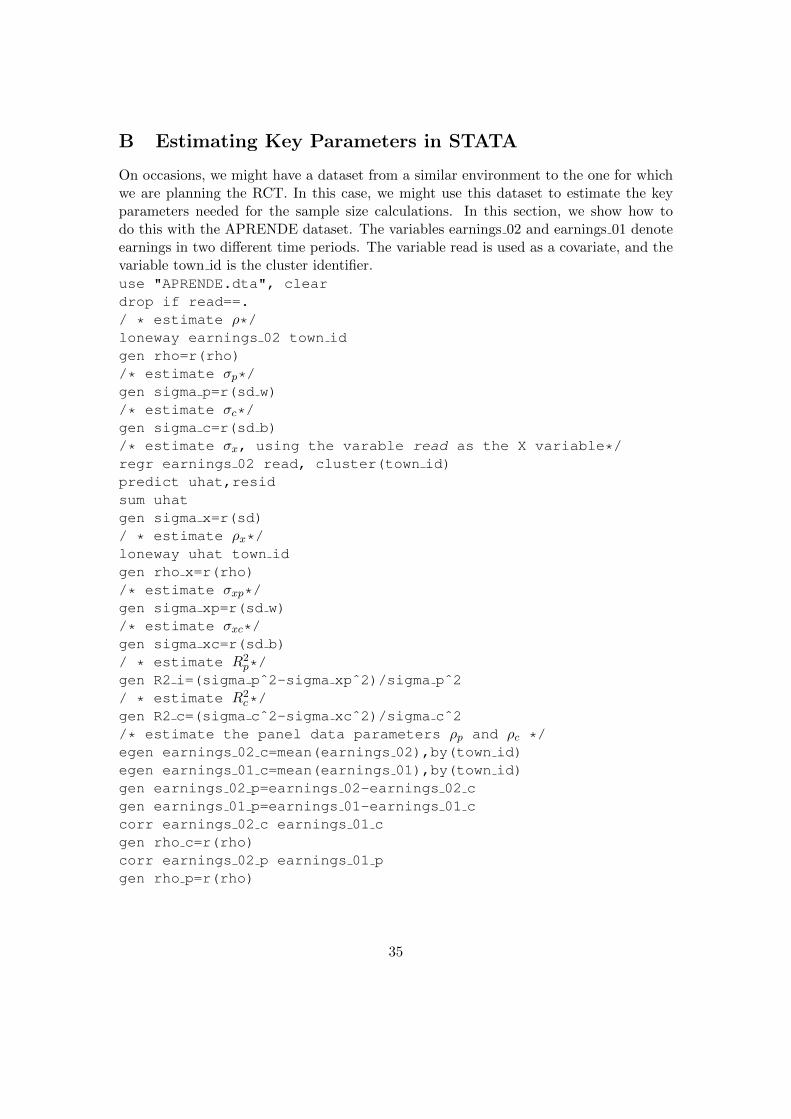
B Estimating Key Parameters in STATA

On occasions, we might have a dataset from a similar environment to the one for whichwe are planning the RCT. In this case, we might use this dataset to estimate the keyparameters needed for the sample size calculations. In this section, we show how todo this with the APRENDE dataset. The variables earnings 02 and earnings 01 denoteearnings in two different time periods. The variable read is used as a covariate, and thevariable town id is the cluster identifier.use "APRENDE.dta", cleardrop if read==./ * estimate ρ*/loneway earnings 02 town idgen rho=r(rho)/* estimate σp*/gen sigma p=r(sd w)/* estimate σc*/gen sigma c=r(sd b)/* estimate σx, using the varable read as the X variable*/regr earnings 02 read, cluster(town id)predict uhat,residsum uhatgen sigma x=r(sd)/ * estimate ρx*/loneway uhat town idgen rho x=r(rho)/* estimate σxp*/gen sigma xp=r(sd w)/* estimate σxc*/gen sigma xc=r(sd b)/ * estimate R2

p*/gen R2 i=(sigma pˆ2-sigma xpˆ2)/sigma pˆ2/ * estimate R2

c*/gen R2 c=(sigma cˆ2-sigma xcˆ2)/sigma cˆ2/* estimate the panel data parameters ρp and ρc */egen earnings 02 c=mean(earnings 02),by(town id)egen earnings 01 c=mean(earnings 01),by(town id)gen earnings 02 p=earnings 02-earnings 02 cgen earnings 01 p=earnings 01-earnings 01 ccorr earnings 02 c earnings 01 cgen rho c=r(rho)corr earnings 02 p earnings 01 pgen rho p=r(rho)

35

C Simulation Code

The objective here is to provide sections of code that are useful if you would like torun your own simulations. This may be done in order to verify formulae for certainoutcomes, or to provide a simulated estimate of sample size if no formulae are availablefor the specific, likely complex, trial design to be implemented.

C.1 How to Create Clusters

The code below creates a dataset with 100 clusters (k = 100) with 10 observations percluster (m = 10), with equal treatment/control allocation. At the cluster level, a nor-mally distributed cluster level error term, with a standard deviation of 10, is created(called group below). As shown later, this will be used to create an ICC.

/*CLUSTER LEVEL*//* create an empty dataset with 100 observations*/set obs 100gen cluster= n/*draw from a normal distribution, with mean 0, standard deviation10 */gen group=rnormal(0,10)sumlocal N=r(N)/*create the treatment variable indicator*/gen treat=0/* allocate half of the cluster to treatment status, the remaininghalf to control*/replace treat=1 if n<=‘N’/2so clustertempfile cluster error g/*create a temporary file for the cluster errors */save ‘cluster error g’,replace/*INDIVIDUAL LEVEL*/clear/*n=mk, so if we require k=100 and m=10, we need n=1000*/set obs 1000/*Generate clusters*/gen u=invnormal(uniform())/*cut the data into 100 equally sized sections*/egen cluster = cut(u), g(100)replace cluster=cluster+1so cluster

*merge in cluster errorsmerge cluster using ‘cluster error g’

36

C.2 How to Generate Data with a Specific ICC

In this section, all of the initial code is the same as before. The addition comes in thebottom lines, when we create the outcome variable, y, as a mix of individual and clusterlevel errors. The code below sets the ICC=.3 . Note too that we set σ = 10, the averageof y in the control group to 10, and δ = 4.

/*CLUSTER LEVEL*/set obs 100gen cluster= n/* set σ = 10 */gen group=rnormal(0,10)sumlocal N=r(N)gen treat=0replace treat=1 if n<=‘N’/2so clustertempfile cluster error gsave ‘cluster error g’,replace/*INDIVIDUAL LEVEL*/ clearset obs 1000gen u=invnormal(uniform())egen cluster = cut(u), g(100)replace cluster=cluster+1so clustermerge cluster using ‘cluster error g’tab mdrop m/* set σ = 10 */gen individual=rnormal(0,10)/*create error term as composite of group and individual error terms,with weights to achieve an ICC=.3*/gen epsilon = (sqrt(.3))*group + (sqrt(.7))*individual/* set y=10 for the control group */gen y=10+ epsilon if treat==0/* generate a δ = 4 */replace y=10+4+epsilon if treat==1

Once the data has been created, we may want to estimate the ICC. This is doneusing STATA’s loneway command. Below we consider the ICC for the control clusters:

loneway y cluster if treat==0

37

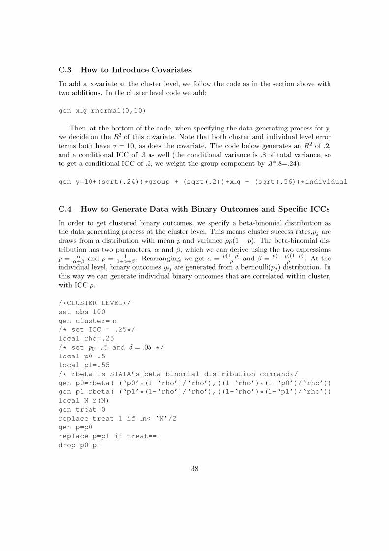
C.3 How to Introduce Covariates

To add a covariate at the cluster level, we follow the code as in the section above withtwo additions. In the cluster level code we add:

gen x g=rnormal(0,10)

Then, at the bottom of the code, when specifying the data generating process for y,we decide on the R2 of this covariate. Note that both cluster and individual level errorterms both have σ = 10, as does the covariate. The code below generates an R2 of .2,and a conditional ICC of .3 as well (the conditional variance is .8 of total variance, soto get a conditional ICC of .3, we weight the group component by .3*.8=.24):

gen y=10+(sqrt(.24))*group + (sqrt(.2))*x g + (sqrt(.56))*individual

C.4 How to Generate Data with Binary Outcomes and Specific ICCs

In order to get clustered binary outcomes, we specify a beta-binomial distribution asthe data generating process at the cluster level. This means cluster success rates,pj aredraws from a distribution with mean p and variance ρp(1 − p). The beta-binomial dis-tribution has two parameters, α and β, which we can derive using the two expressionsp = α

α+β and ρ = 11+α+β . Rearranging, we get α = p(1−ρ)

ρ and β = p(1−p)(1−ρ)ρ . At the

individual level, binary outcomes yij are generated from a bernoulli(pj) distribution. Inthis way we can generate individual binary outcomes that are correlated within cluster,with ICC ρ.

/*CLUSTER LEVEL*/set obs 100gen cluster= n/* set ICC = .25*/local rho=.25/* set p0=.5 and δ = .05 */local p0=.5local p1=.55/* rbeta is STATA’s beta-binomial distribution command*/gen p0=rbeta( (‘p0’*(1-‘rho’)/‘rho’),((1-‘rho’)*(1-‘p0’)/‘rho’))gen p1=rbeta( (‘p1’*(1-‘rho’)/‘rho’),((1-‘rho’)*(1-‘p1’)/‘rho’))local N=r(N)gen treat=0replace treat=1 if n<=‘N’/2gen p=p0replace p=p1 if treat==1drop p0 p1

38

so clustertempfile cluster p gsave ‘cluster p g’,replace/*INDIVIDUAL LEVEL*/clearset obs 1000

* Generate clustersgen u=invnormal(uniform())egen cluster = cut(u), g(100)replace cluster=cluster+1so cluster

*merge in cluster errorsmerge cluster using ‘cluster p g’tab mdrop m/*quick way to generate bernoulli(p) distributed data*/gen y = ( uniform() < p )

C.5 How to Create Panel Data

In this section we detail how to create panel data, with specific autocorrelation and ICCterms. Below, the values are set to ρc = .2, ρp = .7, the ICC ρ = .3, and as before, σ = 10:

/*CLUSTER LEVEL*/set obs 100gen cluster= n/* set σ = 10 */gen grp=rnormal(0,10)gen grp1=rnormal(0,10)gen grp2=rnormal(0,10)/* where we determine ρc */gen group1=sqrt(.2)*grp +sqrt(.8)*grp1gen group2=sqrt(.2)*grp +sqrt(.8)*grp2sumdrop grp*local N=r(N)di ‘N’gen treat=0replace treat=1 if n<=‘N’/2so clustersave cluster error,replace/*INDIVIDUAL LEVEL*/clearset obs 1000

39

* Generate clustersgen u=invnormal(uniform())egen cluster = cut(u), g(100)replace cluster=cluster+1so cluster

*merge in cluster errorsmerge cluster using cluster errortab mdrop m u/* set σ = 10 */gen indv=rnormal(0,10)gen indv1=rnormal(0,10)gen indv2=rnormal(0,10)/* where we determine ρp */gen individual1=sqrt(.7)*indv+sqrt(.3)*indv1gen individual2=sqrt(.7)*indv+sqrt(.3)*indv2drop indv*/* where we set the ICC */gen y0=10+(sqrt(.3))*group1 + (sqrt(.7))*individual1/* allow y to increase by 2 in the second period, a common time trend*/gen y1=12+(sqrt(.3))*group2 + (sqrt(.7))*individual2drop group* individual*/* set δ = 4 */replace y1=y1+4 if treat==1

As part of the simulation, we might want to verify that the data is being generatedwith the correct ρp and ρc. Below is some simple code to estimate these parameters fromthe simulation directly above:

/* construct cluster means of outcome variable */egen y1 cluster=mean(y1),by(cluster)egen y0 cluster=mean(y0),by(cluster)/*construct individual component of outcome variable */gen y1 individual=y1-y1 clustergen y0 individual=y0-y0 cluster/* ρc estimate */corr y1 cluster y0 cluster/* ρp estimate*/corr y1 individual y0 individual

C.6 How to Compute Power Via Simulation

In this section we present code in order to simulate power as detailed in section 6.2.The basic idea here is to run 1000 simulations, and then count the number of times the

40

treatment coefficient is statistically significantly different from zero. Counting the num-ber of times we get a statistically significant parameter, and dividing it by 1000 yieldsour simulated power. In the code below, we refer to the seven steps outlined in section6.2 in order to outline how one may proceed with simulating power. The example belowis for a continuous outcome with cluster randomised treatment.

/*STEP 1*/local numits=1000local it=0/ create a temporary file that will store the output from the simulations

*/tempname memholdtempfile montec resultspostfile ‘memhold’ reject t rho using ‘montec results’/* start quietly */qui{/*start iterations here*/while ‘it’<=‘numits’{local it=‘it’+1clear/* STEPS 2 and 3 */

*cluster errorsset obs 100gen cluster= ngen group=rnormal(0,10)sumlocal N=r(N)di ‘N’gen treat=0replace treat=1 if n<=‘N’/2so clustertempfile cluster error gsave ‘cluster error g’,replaceclearset obs 1000

* Generate clustersgen u=invnormal(uniform())egen cluster = cut(u), g(100)replace cluster=cluster+1so cluster

*merge in cluster errorsmerge cluster using ‘cluster error g’tab m

41

drop mgen individual=rnormal(0,10)/* STEP 4*/gen y=10+(sqrt(.3))*group + (sqrt(.7))*individualreplace y=y+4 if treat==1loneway y cluster if treat==0local rho=r(rho)regr y treat,cluster(cluster)/* STEP 5 */local t loop= b[treat]/ se[treat]local df=100local critical u=invttail(‘df’,.05/2)local critical l=invttail(‘df’,1-.05/2)local reject t=(‘t loop’>‘critical u’)|(‘t loop’<‘critical l’)di ‘reject t’/*write output from simulation to the temporary file*/post ‘memhold’ (‘reject t’) (‘rho’)clear}/* STEP 6 */} /* close quietly*/postclose ‘memhold’use ‘montec results’,clear/* STEP 7 *//* reject=1 if null is rejected, 0 otherwise. So the mean of rejectfrom the 1000 simulation draws will yield the simulated power */sum reject t rho

D STATA Programmes to Compute Power with BinaryOutcomes

Below is some code that creates a STATA .ado programme in order to get power forbinary outcomes. The first section of code immediately below is for the case where thereare no covariates:

cap prog drop discretepowerprogram discretepowersyntax anything [,alpha(real .05) beta(real .8) pi(real .5)]tokenize "‘0’",parse(" ,")local rho =‘1’local m =‘2’local p 0 =‘3’local impact =‘4’

42

local z alpha = invnormal(1-(‘alpha’/2))local z beta = invnormal(‘beta’)local deff = (1+‘rho’*(‘m’-1))local p 1 =‘p 0’+‘impact’local k =(‘deff’/‘m’)*( (‘p 1’*(1-‘p 1’)/‘pi’)+(‘p 0’*(1-‘p 0’)/(1-‘pi’))) *((‘z alpha’+‘z beta’)ˆ2)/‘impact’ˆ2didi "Total number of clusters= " ‘k’end

Here is an example of how to use this .ado file for the case where p0 = 0.5, δ = .1,ρ = .05 and m = 30. The order in which these parameters must be entered is specifiedby the positional arguments within the .ado file. For example, see the line local rho=‘1’

. This tells us that the value of ρ should be entered first. Looking at the proceedinglines, we also see that the order of the remaining parameters are to be entered is m, p0and finally the effect size δ. Looking at the third line of code above (starting with theword syntax), there are several options that may be changed from the default values -α (set at .05), β (set at .8) and π (set at .5):

discretepower .05 30 .5 .1

Now for the more complicated code below, where we allow a single discrete covari-ate, as we saw in section 5.3. The code below allows for a discrete X with five points ofsupport. The code could easily be shortened for a simple binary X, or extended for morepoints of support. The code for points of support up to 5 is supplied as supplementarymaterial:

cap prog drop discretepowerXprogram discretepowerXsyntax anything [,alpha(real .05) beta(real .8) pi(real .5)]tokenize "‘0’",parse(" ,")local rho =‘1’local m =‘2’local x 0 =‘3’local theta 0 =‘4’local p C0 =‘5’local impact 0 =‘6’local x 1 =‘7’local theta 1 =‘8’local p C1 =‘9’local impact 1 =‘10’local x 2 =‘11’

43

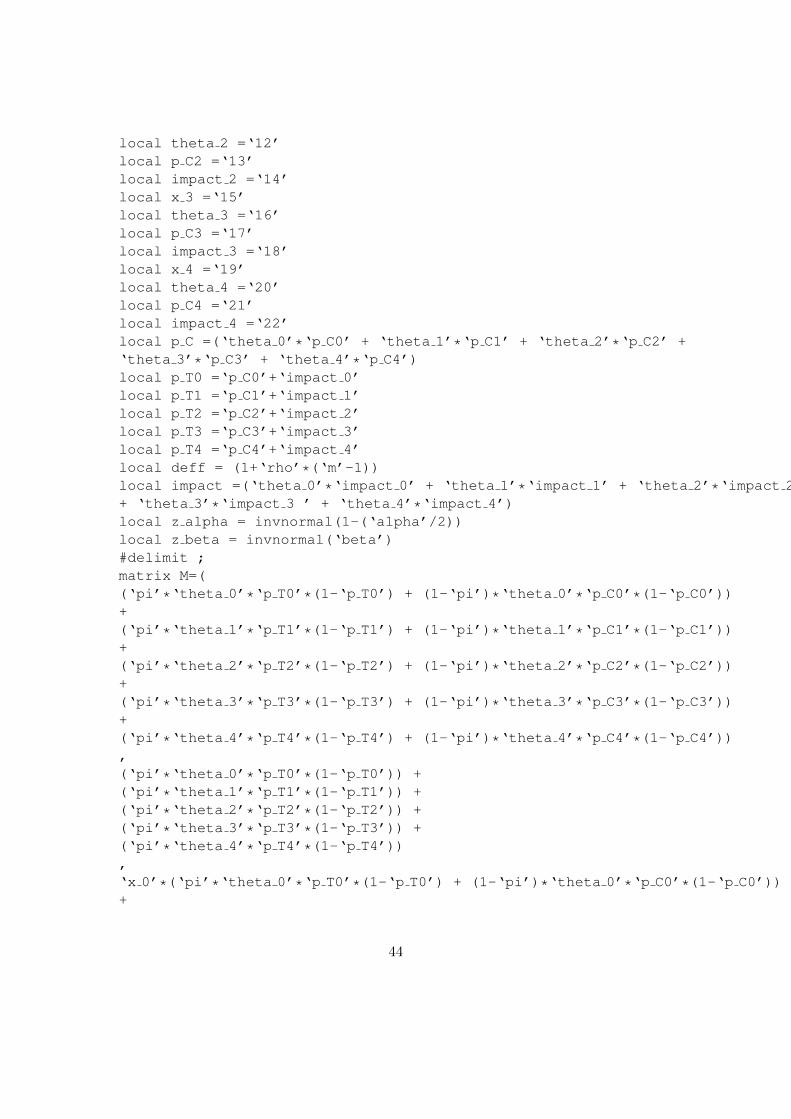
local theta 2 =‘12’local p C2 =‘13’local impact 2 =‘14’local x 3 =‘15’local theta 3 =‘16’local p C3 =‘17’local impact 3 =‘18’local x 4 =‘19’local theta 4 =‘20’local p C4 =‘21’local impact 4 =‘22’local p C =(‘theta 0’*‘p C0’ + ‘theta 1’*‘p C1’ + ‘theta 2’*‘p C2’ +‘theta 3’*‘p C3’ + ‘theta 4’*‘p C4’)local p T0 =‘p C0’+‘impact 0’local p T1 =‘p C1’+‘impact 1’local p T2 =‘p C2’+‘impact 2’local p T3 =‘p C3’+‘impact 3’local p T4 =‘p C4’+‘impact 4’local deff = (1+‘rho’*(‘m’-1))local impact =(‘theta 0’*‘impact 0’ + ‘theta 1’*‘impact 1’ + ‘theta 2’*‘impact 2’+ ‘theta 3’*‘impact 3 ’ + ‘theta 4’*‘impact 4’)local z alpha = invnormal(1-(‘alpha’/2))local z beta = invnormal(‘beta’)#delimit ;matrix M=((‘pi’*‘theta 0’*‘p T0’*(1-‘p T0’) + (1-‘pi’)*‘theta 0’*‘p C0’*(1-‘p C0’))+(‘pi’*‘theta 1’*‘p T1’*(1-‘p T1’) + (1-‘pi’)*‘theta 1’*‘p C1’*(1-‘p C1’))+(‘pi’*‘theta 2’*‘p T2’*(1-‘p T2’) + (1-‘pi’)*‘theta 2’*‘p C2’*(1-‘p C2’))+(‘pi’*‘theta 3’*‘p T3’*(1-‘p T3’) + (1-‘pi’)*‘theta 3’*‘p C3’*(1-‘p C3’))+(‘pi’*‘theta 4’*‘p T4’*(1-‘p T4’) + (1-‘pi’)*‘theta 4’*‘p C4’*(1-‘p C4’)),(‘pi’*‘theta 0’*‘p T0’*(1-‘p T0’)) +(‘pi’*‘theta 1’*‘p T1’*(1-‘p T1’)) +(‘pi’*‘theta 2’*‘p T2’*(1-‘p T2’)) +(‘pi’*‘theta 3’*‘p T3’*(1-‘p T3’)) +(‘pi’*‘theta 4’*‘p T4’*(1-‘p T4’)),‘x 0’*(‘pi’*‘theta 0’*‘p T0’*(1-‘p T0’) + (1-‘pi’)*‘theta 0’*‘p C0’*(1-‘p C0’))+

44

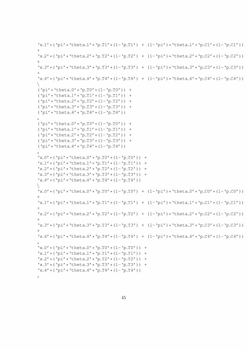
‘x 1’*(‘pi’*‘theta 1’*‘p T1’*(1-‘p T1’) + (1-‘pi’)*‘theta 1’*‘p C1’*(1-‘p C1’))+‘x 2’*(‘pi’*‘theta 2’*‘p T2’*(1-‘p T2’) + (1-‘pi’)*‘theta 2’*‘p C2’*(1-‘p C2’))+‘x 3’*(‘pi’*‘theta 3’*‘p T3’*(1-‘p T3’) + (1-‘pi’)*‘theta 3’*‘p C3’*(1-‘p C3’))+‘x 4’*(‘pi’*‘theta 4’*‘p T4’*(1-‘p T4’) + (1-‘pi’)*‘theta 4’*‘p C4’*(1-‘p C4’))\(‘pi’*‘theta 0’*‘p T0’*(1-‘p T0’)) +(‘pi’*‘theta 1’*‘p T1’*(1-‘p T1’)) +(‘pi’*‘theta 2’*‘p T2’*(1-‘p T2’)) +(‘pi’*‘theta 3’*‘p T3’*(1-‘p T3’)) +(‘pi’*‘theta 4’*‘p T4’*(1-‘p T4’)),(‘pi’*‘theta 0’*‘p T0’*(1-‘p T0’)) +(‘pi’*‘theta 1’*‘p T1’*(1-‘p T1’)) +(‘pi’*‘theta 2’*‘p T2’*(1-‘p T2’)) +(‘pi’*‘theta 3’*‘p T3’*(1-‘p T3’)) +(‘pi’*‘theta 4’*‘p T4’*(1-‘p T4’)),‘x 0’*(‘pi’*‘theta 0’*‘p T0’*(1-‘p T0’)) +‘x 1’*(‘pi’*‘theta 1’*‘p T1’*(1-‘p T1’)) +‘x 2’*(‘pi’*‘theta 2’*‘p T2’*(1-‘p T2’)) +‘x 3’*(‘pi’*‘theta 3’*‘p T3’*(1-‘p T3’)) +‘x 4’*(‘pi’*‘theta 4’*‘p T4’*(1-‘p T4’))\‘x 0’*(‘pi’*‘theta 0’*‘p T0’*(1-‘p T0’) + (1-‘pi’)*‘theta 0’*‘p C0’*(1-‘p C0’))+‘x 1’*(‘pi’*‘theta 1’*‘p T1’*(1-‘p T1’) + (1-‘pi’)*‘theta 1’*‘p C1’*(1-‘p C1’))+‘x 2’*(‘pi’*‘theta 2’*‘p T2’*(1-‘p T2’) + (1-‘pi’)*‘theta 2’*‘p C2’*(1-‘p C2’))+‘x 3’*(‘pi’*‘theta 3’*‘p T3’*(1-‘p T3’) + (1-‘pi’)*‘theta 3’*‘p C3’*(1-‘p C3’))+‘x 4’*(‘pi’*‘theta 4’*‘p T4’*(1-‘p T4’) + (1-‘pi’)*‘theta 4’*‘p C4’*(1-‘p C4’)),‘x 0’*(‘pi’*‘theta 0’*‘p T0’*(1-‘p T0’)) +‘x 1’*(‘pi’*‘theta 1’*‘p T1’*(1-‘p T1’)) +‘x 2’*(‘pi’*‘theta 2’*‘p T2’*(1-‘p T2’)) +‘x 3’*(‘pi’*‘theta 3’*‘p T3’*(1-‘p T3’)) +‘x 4’*(‘pi’*‘theta 4’*‘p T4’*(1-‘p T4’)),

45

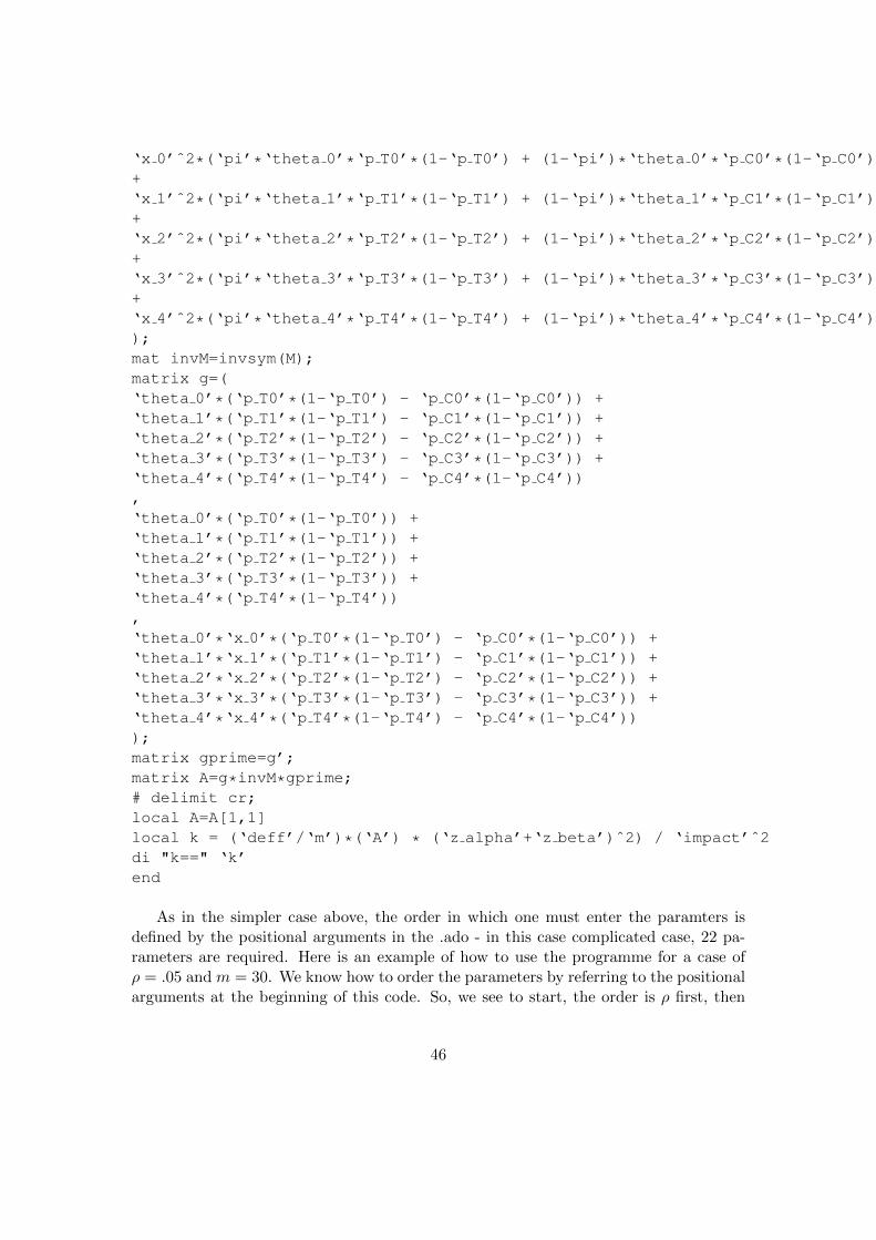
‘x 0’ˆ2*(‘pi’*‘theta 0’*‘p T0’*(1-‘p T0’) + (1-‘pi’)*‘theta 0’*‘p C0’*(1-‘p C0’))+‘x 1’ˆ2*(‘pi’*‘theta 1’*‘p T1’*(1-‘p T1’) + (1-‘pi’)*‘theta 1’*‘p C1’*(1-‘p C1’))+‘x 2’ˆ2*(‘pi’*‘theta 2’*‘p T2’*(1-‘p T2’) + (1-‘pi’)*‘theta 2’*‘p C2’*(1-‘p C2’))+‘x 3’ˆ2*(‘pi’*‘theta 3’*‘p T3’*(1-‘p T3’) + (1-‘pi’)*‘theta 3’*‘p C3’*(1-‘p C3’))+‘x 4’ˆ2*(‘pi’*‘theta 4’*‘p T4’*(1-‘p T4’) + (1-‘pi’)*‘theta 4’*‘p C4’*(1-‘p C4’)));mat invM=invsym(M);matrix g=(‘theta 0’*(‘p T0’*(1-‘p T0’) - ‘p C0’*(1-‘p C0’)) +‘theta 1’*(‘p T1’*(1-‘p T1’) - ‘p C1’*(1-‘p C1’)) +‘theta 2’*(‘p T2’*(1-‘p T2’) - ‘p C2’*(1-‘p C2’)) +‘theta 3’*(‘p T3’*(1-‘p T3’) - ‘p C3’*(1-‘p C3’)) +‘theta 4’*(‘p T4’*(1-‘p T4’) - ‘p C4’*(1-‘p C4’)),‘theta 0’*(‘p T0’*(1-‘p T0’)) +‘theta 1’*(‘p T1’*(1-‘p T1’)) +‘theta 2’*(‘p T2’*(1-‘p T2’)) +‘theta 3’*(‘p T3’*(1-‘p T3’)) +‘theta 4’*(‘p T4’*(1-‘p T4’)),‘theta 0’*‘x 0’*(‘p T0’*(1-‘p T0’) - ‘p C0’*(1-‘p C0’)) +‘theta 1’*‘x 1’*(‘p T1’*(1-‘p T1’) - ‘p C1’*(1-‘p C1’)) +‘theta 2’*‘x 2’*(‘p T2’*(1-‘p T2’) - ‘p C2’*(1-‘p C2’)) +‘theta 3’*‘x 3’*(‘p T3’*(1-‘p T3’) - ‘p C3’*(1-‘p C3’)) +‘theta 4’*‘x 4’*(‘p T4’*(1-‘p T4’) - ‘p C4’*(1-‘p C4’)));matrix gprime=g’;matrix A=g*invM*gprime;# delimit cr;local A=A[1,1]local k = (‘deff’/‘m’)*(‘A’) * (‘z alpha’+‘z beta’)ˆ2) / ‘impact’ˆ2di "k==" ‘k’end

As in the simpler case above, the order in which one must enter the paramters isdefined by the positional arguments in the .ado - in this case complicated case, 22 pa-rameters are required. Here is an example of how to use the programme for a case ofρ = .05 and m = 30. We know how to order the parameters by referring to the positionalarguments at the beginning of this code. So, we see to start, the order is ρ first, then

46

m, then x0, followed by θ0 and so on for the remaining 18 parameters:

discretepowerX 0.05 30 -2 .2 .1 0 -1 .2 .4 .05 0 .2 .5 .1 1 .2 .6.15 2 .2 .9 .2

To clarify, the full syntax for this prgramme is:discretepowerX ρ m x0 θ0 pC0 δ0 x1 θ1 pC1 δ1 x2 θ2 pC2 δ2 x3 θ3 pC3 δ3 x4θ4 pC4 δ4

E STATA Optimisation Programme to Solve for OptimalSample Allocation Under A Complex Cost Function

This programme uses MATA’s optimize routine to solve for the optimal sample alloca-tion when facing a complex cost function. This entails minimising the objective function(σ2ck0

+σ2p

m0k0+ σ2

ck1

+σ2p

m1k1

)subject to the complex cost function C = k0(f0 + v0m0) +

k1(f1 + v1m1). This is operationalised by rearranging the cost function so that m0 is onthe left-hand side, and then using this function to replace m0 in the objective function.The optimisation function below thus solves for m∗1, k

∗0 and k∗1, and then m∗0 is calculated

from the cost function.

clearset obs 1gen k0=.gen k1=.gen m1=.local f0=6.5local f1=12.25local C=50000local m=20local v0=2local v1=7local sigma=126383.5local rho=.05local sigmap2=(1-‘rho’)*(‘sigma’ˆ2)local sigmac2=‘rho’*(‘sigma’ˆ2)/*here optimising over 3 unknowns:ko , k1 and m1x[1], x[2] and x[3]

*/mata: mata clear

47

mata: mata set matastrict offmatavoid myeval(todo, x, y, g, H)y = ‘sigmac2’/x[1]+‘sigmap2’/(x[1]*((‘C’-‘f0’*x[1] - (‘f1’+‘v1’*x[3])*x[2])/(‘v0’*x[1])))+ ‘sigmac2’/(x[2])+‘sigmap2’/(x[3]*x[2])S = optimize init()optimize init which(S,"min" )optimize init evaluator(S, &myeval())optimize init params(S, (930,600,6))x = optimize(S)xst store(., "k0", x[1,1])st store(., "k1", x[1,2])st store(., "m1", x[1,3])endlocal k0=k0[1]local k1=k1[1]local m1=m1[1]local m0=((‘C’-‘f0’*‘k0’ - (‘f1’+‘v1’*‘m1’)*‘k1’)/(‘v0’*‘k0’))di ‘k1’di ‘k0’di ‘m1’di ‘m0’/* internal consistency check to ensure that optimal parameters yieldthe total cost (here C=50000) when inputted into the cost function

*/di ‘k0’*(‘f0’+‘v0’*‘m0’)+‘k1’*(‘f1’+‘v1’*‘m1’)

48

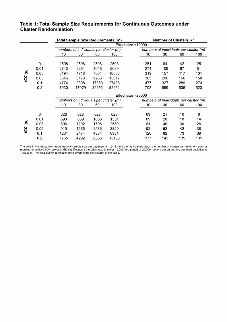
Total Sample Size Requirements (n*) Number of Clusters, k*Effect size =10000

numbers of individuals per cluster (m) numbers of individuals per cluster (m)10 30 60 100 10 30 60 100

ICC

(ρ

)

0 2508 2508 2508 2508 251 84 42 250.01 2743 3264 4046 5089 274 109 67 510.03 3194 4718 7004 10053 319 157 117 1010.05 3646 6173 9963 15017 365 206 166 1500.1 4774 9808 17360 27428 477 327 289 2740.2 7030 17079 32153 52251 703 569 536 523

Effect size =20000numbers of individuals per cluster (m) numbers of individuals per cluster (m)

10 30 60 100 10 30 60 100

ICC

(ρ

)

0 628 628 628 628 63 21 10 60.01 693 839 1058 1351 69 28 18 140.03 806 1202 1796 2589 81 40 30 260.05 919 1565 2536 3829 92 52 42 380.1 1201 2474 4384 6931 120 82 73 690.2 1765 4292 8083 13136 177 143 135 131

Table 1: Total Sample Size Requirements for Continuous Outcomes under Cluster Randomisation

The cells in the left panels report the total sample size per treatment arm (m*k) and the right panels report the number of clusters per treatment arm (k) required to achieve 80% power at 5% significance if the effect size is either 10,000 (top panel) or 20,000 (bottom panel) and the standard deviation is 126383.5. The intra cluster correlation (ρ) is given in the first column of the Table.

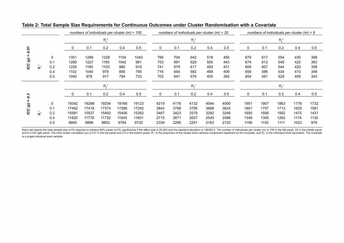
Table 2: Total Sample Size Requirements for Continuous Outcomes under Cluster Randomisation with a Covariate

numbers of individuals per cluster (m) = 100 numbers of individuals per cluster (m) = 20 numbers of individuals per cluster (m) = 8IC

C (

ρ)

= 0

.01 0 0.1 0.2 0.4 0.5 0 0.1 0.2 0.4 0.5 0 0.1 0.2 0.4 0.5

0 1351 1289 1228 1104 1043 766 704 642 518 456 679 617 554 430 3680.1 1289 1227 1165 1042 981 753 691 629 505 443 674 612 549 425 3630.2 1226 1165 1103 980 919 741 679 617 493 431 669 607 544 420 3580.4 1102 1040 979 856 795 716 654 592 468 406 659 596 534 410 3480.5 1040 978 917 794 733 703 641 579 455 393 654 591 529 405 343

ICC

(ρ

) =

0.3 0 0.1 0.2 0.4 0.5 0 0.1 0.2 0.4 0.5 0 0.1 0.2 0.4 0.5

0 19342 19298 19254 19166 19123 4219 4176 4132 4044 4000 1951 1907 1863 1776 17320.1 17462 17418 17374 17286 17242 3843 3799 3756 3668 3624 1801 1757 1713 1625 15810.2 15581 15537 15493 15406 15362 3467 3423 3379 3292 3248 1650 1606 1562 1475 14310.4 11820 11776 11732 11645 11601 2715 2671 2627 2540 2496 1349 1305 1262 1174 11300.5 9940 9896 9852 9764 9720 2339 2295 2251 2163 2120 1199 1155 1111 1023 979

Rp2 R

p2 R

p2

Rc2

Rp2 R

p2 R

p2

Rc2

Each cell reports the total sample size (m*k) required to achieve 80% power at 5% significance if the effect size is 20,000 and the standard deviation is 126383.5. The number of individuals per cluster (m) is 100 in the left panel, 20 in the middle panel and 8 in the right panel. The intra cluster correlation (ρ) is 0.01 in the top panel and 0.3 in the bottom panel. Rc

2 is the proportion of the cluster level variance component explained by the covariate, and Rp2 is the individual level equivalent. The covariate

is a single individual level variable.

Difference

r0.1 4909 8820 4860

0.25 4909 7354 46030.5 4909 4909 3687

0.75 4909 2464 21590.9 4909 998 949

Table 3: Sample size Requirements for Continuous Outcomes in Panel Data Models

Difference-in-differences

Lagged Outcome

The ICC is .05 and the number of individuals per cluster, m, is set to 20. The effect size is equal to 10000 and the standard deviation is 126383.5

Total Sample Size Requirements (N*) Number of Clusters (2k*)

Control Group Success Rate (p0): 0.1

numbers of individuals per cluster (m) numbers of individuals per cluster (m)10 30 60 100 10 30 60 100

ICC

0 392 392 392 392 39 13 7 40.01 428 506 624 781 43 17 10 80.03 498 734 1087 1558 50 24 18 160.05 569 961 1550 2335 57 32 26 230.1 746 1531 2708 4278 75 51 45 430.2 1099 2669 5023 8163 110 89 84 82

Control Group Success Rate (p0): 0.3

numbers of individuals per cluster (m) numbers of individuals per cluster (m)10 30 60 100 10 30 60 100

ICC

0 706 706 706 706 71 24 12 70.01 770 911 1123 1406 77 30 19 140.03 897 1321 1957 2804 90 44 33 280.05 1024 1731 2790 4203 102 58 47 420.1 1342 2755 4874 7700 134 92 81 770.2 1978 4804 9042 14693 198 160 151 147

Control Group Success Rate (p0): 0.5

numbers of individuals per cluster (m) numbers of individuals per cluster (m)10 30 60 100 10 30 60 100

ICC

0 769 769 769 769 77 26 13 80.01 838 992 1223 1531 84 33 20 150.03 977 1438 2131 3054 98 48 36 310.05 1115 1885 3038 4577 112 63 51 460.1 1461 3000 5307 8384 146 100 88 840.2 2154 5230 9846 15999 215 174 164 160

Effect size is set to .1 and treatment is evenly allocated (π=.5).

Table 4: Sample Size Requirements for Binary Outcomes Under Cluster Randomisation

ICC=.05 ICC=.1

.1/.1 .05/.15 .03/.17 .1/.1 .05/.15 .03/.17

.45/.55 50 49 49 88 86 85.4/.6 49 47 47 85 83 81.3/.7 42 40 39 74 70 68.2/.8 32 29 27 56 50 47

Table 5: Number of Clusters Required for Binary Outcomes Under Cluster Randomisation With A Binary Covariate

Control group success rates for

Xj=0/X

j=1

Impacts for Xj=0/X

j=1 Impacts for X

j=0/X

j=1

Number of individuals per cluster, m, is set at 60. The overall base rate in this table is set to .5, with the overall impact set to .1. Treatment is evenly allocated (π=.5), and θ= P(Xj=1)=.5.

Table 6: Optimal Cost Calculations for Individually Randomised Treatment

50 50 50 50 50 50 50 50

50 75 100 150 200 250 300 500

Sample 2508 2790 3028 3426 3762 4058 4326 5220

2508 2278 2141 1978 1881 1815 1766 1651

Optimal Total Cost (C* ) 250835 310374 365488 468051 564353 656656 746117 1086285

250835 313543 376252 501669 627086 752504 877921 1379590

Cost Savings 0% 1% 3% 7% 10% 13% 15% 21%

Unit cost Control (c0)

Unit cost Treatment (c1)

Control (n0)

Treatment (n1)

Total Cost Under Even Sample Split (n0=n

1)

Here, the unit cost for control individuals represents the cost of data collection. The unit cost of treatment additionally incorporates the intervention cost. For all calculations, the effect size is set to 10000, and the standard deviation is 126383.5. Power is set to 80% power and the significance level at 5%. No covariates are included.