Go-Explore: a New Approach for Hard-ExplorationProblems

Adrien Ecoffet Joost Huizinga Joel Lehman Kenneth O. Stanley* Jeff Clune*Uber AI Labs

San Francisco, CA 94103adrienecoffet,joost.hui,jclune@gmail.com

*Co-senior authors

Authors’ note: We recommend reading (and citing) our updated paper, “First return, then explore”:

Ecoffet, A., Huizinga, J., Lehman, J., Stanley, K.O. and Clune, J. First return, then explore. Nature590, 580–586 (2021). https://doi.org/10.1038/s41586-020-03157-9

It can be found at https://tinyurl.com/Go-Explore-Nature.

Abstract

A grand challenge in reinforcement learning is intelligent exploration, especiallywhen rewards are sparse or deceptive. Two Atari games serve as benchmarks forsuch hard-exploration domains: Montezuma’s Revenge and Pitfall. On both games,current RL algorithms perform poorly, even those with intrinsic motivation, whichis the dominant method to encourage exploration and improve performance on hard-exploration domains. To address this shortfall, we introduce a new algorithm calledGo-Explore. It exploits the following principles: (1) remember states that havepreviously been visited, (2) first return to a promising state (without exploration),then explore from it, and (3) solve simulated environments through exploiting anyavailable means (including by introducing determinism), then robustify (create apolicy that can reliably perform the solution) via imitation learning. The combinedeffect of these principles generates dramatic performance improvements on hard-exploration problems. On Montezuma’s Revenge, without being provided anydomain knowledge, Go-Explore scores over 43,000 points, almost 4 times theprevious state of the art. Go-Explore can also easily harness human-provideddomain knowledge, and when augmented with it Go-Explore scores a mean ofover 650,000 points on Montezuma’s Revenge. Its max performance of 18 millionsurpasses the human world record by an order of magnitude, thus meeting eventhe strictest definition of “superhuman” performance. On Pitfall, Go-Explore withdomain knowledge is the first algorithm to score above zero. Its mean performanceof almost 60,000 points also exceeds expert human performance. Because Go-Explore can produce many high-performing demonstrations automatically andcheaply, it also outperforms previous imitation learning work in which the solutionwas provided in the form of a human demonstration. Go-Explore opens up manynew research directions into improving it and weaving its insights into current RLalgorithms. It may also enable progress on previously unsolvable hard-explorationproblems in a variety of domains, especially the many that often harness a simulatorduring training (e.g. robotics).

1 Introduction

Reinforcement learning (RL) has experienced significant progress in recent years, achieving super-human performance in board games such as Go [1, 2] and in classic video games such as Atari [3].However, this progress obscures some of the deep unmet challenges in scaling RL to complex

arX

iv:1

901.

1099

5v4

[cs

.LG

] 2

6 Fe

b 20

21

real-world domains. In particular, many important tasks require effective exploration to be solved, i.e.to explore and learn about the world even when rewards are sparse or deceptive. In sparse-rewardproblems, precise sequences of many (e.g. hundreds or more) actions must be taken between ob-taining rewards. Deceptive-reward problems are even harder, because instead of feedback rarelybeing provided, the reward function actually provides misleading feedback for reaching the overallglobal objective, which can lead to getting stuck on local optima. Both sparse and deceptive rewardproblems constitute “hard-exploration” problems, and classic RL algorithms perform poorly onthem [4]. Unfortunately, most challenging real-world problems are also hard-exploration problems.That is because we often desire to provide abstract goals (e.g. “find survivors and tell us their location,”or “turn off the valve to the leaking pipe in the reactor”), and such reward functions do not providedetailed guidance on how to solve the problem (sparsity) while also often creating unintended localoptima (deception) [5–8].

For example, in the case of finding survivors in a disaster area, survivors will be few and far between,thus introducing sparsity. Even worse, if we also instruct the robot to minimize damage to itself,this additional reward signal may actively teach the robot not to explore the environment, becauseexploration is initially much more likely to result in damage than it is to result in finding a survivor.This seemingly sensible additional objective thus introduces deception on top of the already sparsereward problem.

To address these challenges, this paper introduces Go-Explore, a new algorithm for hard-explorationproblems that dramatically improves state-of-the-art performance in two classic hard-explorationbenchmarks: the Atari games Montezuma’s Revenge and Pitfall.

Prior to Go-Explore, the typical approach to sparse reward problems has been intrinsic motivation(IM) [4, 9–11], which supplies the RL agent with intrinsic rewards (IRs) that encourage exploration(augmenting or replacing extrinsic reward that comes from the environment). IM is often motivated bypsychological concepts such as curiosity [12, 13] or novelty-seeking [7, 14], which play a role in howhumans explore and learn. While IM has produced exciting progress in sparse reward problems, inmany domains IM approaches are still far from fully solving the problem, including on Montezuma’sRevenge and Pitfall. We hypothesize that, amongst other issues, such failures stem from two rootcauses that we call detachment and derailment.

Detachment is the idea that an agent driven by IM could become detached from the frontiers ofhigh intrinsic reward (IR). To understand detachment, we must first consider that intrinsic rewardis nearly always a consumable resource: a curious agent is curious about states to the extent that ithas not often visited them (similar arguments apply for surprise, novelty, or prediction-error seekingagents [4, 14–16]). If an agent discovers multiple areas of the state space that produce high IR, itspolicy may in the short term focus on one such area. After exhausting some of the IR offered by thatarea, the policy may by chance begin consuming IR in another area. Once it has exhausted that IR, itis difficult for it to rediscover the frontier it detached from in the initial area, because it has alreadyconsumed the IR that led to that frontier (Fig. 1), and it likely will not remember how to return tothat frontier due to catastrophic forgetting [17–20]. Each time this process occurs, a potential avenueof exploration can be lost, or at least be difficult to rediscover. In the worst case, there may be adearth of remaining IR near the areas of state space visited by the current policy (even though muchIR might remain elsewhere), and therefore no learning signal remains to guide the agent to furtherexplore in an effective and informed way. One could slowly add intrinsic rewards back over time,but then the entire fruitless process could repeat indefinitely. In theory a replay buffer could preventdetachment, but in practice it would have to be large to prevent data about the abandoned frontier tonot be purged before it becomes needed, and large replay buffers introduce their own optimizationstability difficulties [21, 22]. The Go-Explore algorithm addresses detachment by explicitly storingan archive of promising states visited so that they can then be revisited and explored from later.

Derailment can occur when an agent has discovered a promising state and it would be beneficialto return to that state and explore from it. Typical RL algorithms attempt to enact such desirablebehavior by running the policy that led to the initial state again, but with some stochastic perturbationsto the existing policy mixed in to encourage a slightly different behavior (e.g. exploring further). Thestochastic perturbation is performed because IM agents have two layers of exploration mechanisms:(1) the higher-level IR incentive that rewards when new states are reached, and (2) a more basicexploratory mechanism such as epsilon-greedy exploration, action-space noise, or parameter-spacenoise [23–25]. Importantly, IM agents rely on the latter mechanism to discover states containing

2

Figure 1: A hypothetical example of detachment in intrinsic motivation (IM) algorithms. Greenareas indicate intrinsic reward, white indicates areas where no intrinsic reward remains, and purpleareas indicate where the algorithm is currently exploring. (1) The agent starts each episode betweenthe two mazes. (2) It may by chance start exploring the West maze and IM may drive it to learn totraverse, say, 50% of it. (3) Because current algorithms sprinkle in randomness (either in actions orparameters) to try to produce new behaviors to find explicit or intrinsic rewards, by chance the agentmay at some point begin exploring the East maze, where it will also encounter a lot of intrinsic reward.After completely exploring the East maze, it has no explicit memory of the promising explorationfrontier it abandoned in the West maze. It likely would also have no implicit memory of this frontierdue to the problem of catastrophic forgetting [17–20]. (4) Worse, the path leading to the frontier inthe West maze has already been explored, so no (or little) intrinsic motivation remains to rediscoverit. We thus say the algorithm has detached from a frontier of states that provide intrinsic motivation.As a result, exploration can stall when areas close to where the current agent visits have alreadybeen explored. This problem would be remedied if the agent remembered and returned to previouslydiscovered promising areas for exploration, which Go-Explore does.

Phase 1: explore until solved Phase 2: robustify(if necessary)

Go to stateExplore

from stateUpdate archive

Run imitation learningon best trajectory

Select statefrom archive

Figure 2: A high-level overview of the Go-Explore algorithm.

high IR, and the former mechanism to return to them. However, the longer, more complex, and moreprecise a sequence of actions needs to be in order to reach a previously-discovered high-IR state,the more likely it is that such stochastic perturbations will “derail” the agent from ever returning tothat state. That is because the needed precise actions are naively perturbed by the basic explorationmechanism, causing the agent to only rarely succeed in reaching the known state to which it is drawn,and from which further exploration might be most effective. To address derailment, an insight inGo-Explore is that effective exploration can be decomposed into first returning to a promising state(without intentionally adding any exploration) before then exploring further.

Go-Explore is an explicit response to both detachment and derailment that is also designed to achieverobust solutions in stochastic environments. The version presented here works in two phases (Fig. 2):(1) first solve the problem in a way that may be brittle, such as solving a deterministic version of theproblem (i.e. discover how to solve the problem at all), and (2) then robustify (i.e. train to be able to

3

reliably perform the solution in the presence of stochasticity).1 Similar to IM algorithms, Phase 1focuses on exploring infrequently visited states, which forms the basis for dealing with sparse-rewardand deceptive problems. In contrast to IM algorithms, Phase 1 addresses detachment and derailmentby accumulating an archive of states and ways to reach them through two strategies: (a) add allinterestingly different states visited so far into the archive, and (b) each time a state from the archiveis selected to explore from, first Go back to that state (without adding exploration), and then Explorefurther from that state in search of new states (hence the name “Go-Explore”).

An analogy of searching a house can help one contrast IM algorithms and Phase 1 of Go-Explore.IM algorithms are akin to searching through a house with a flashlight, which casts a narrow beam ofexploration first in one area of the house, then another, and another, and so on, with the light beingdrawn towards areas of intrinsic motivation at the edge of its small visible region. It can get lost if atany point the beam fails to fall on any area with intrinsic motivation remaining. Go-Explore moreresembles turning the lights on in one room of a house, then its adjacent rooms, then their adjacentrooms, etc., until the entire house is illuminated. Go-Explore thus gradually expands its sphere ofknowledge in all directions simultaneously until a solution is discovered.

If necessary, the second phase of Go-Explore robustifies high-performing trajectories from the archivesuch that they are robust to the stochastic dynamics of the true environment. Go-Explore robustifiesvia imitation learning (aka learning from demonstrations or LfD [26–29]), a technique that learns howto solve a task from human demonstrations. The only difference with Go-Explore is that the solutiondemonstrations are produced automatically by Phase 1 of Go-Explore instead of being providedby humans. The input to this phase is one or more high-performing trajectories, and the output isa robust policy able to consistently achieve similar performance. The combination of both phasesinstantiates a powerful algorithm for hard-exploration problems, able to deeply explore sparse- anddeceptive-reward environments and robustify high-performing trajectories into reliable solutions thatperform well in the unmodified, stochastic test environment.

Some of these ideas are similar to ideas proposed in related work. Those connections are discussed inSection 5. That said, we believe we are the first to combine these ideas in this way and demonstratethat doing so provides substantial performance improvements on hard-exploration problems.

To explore its potential, we test Go-Explore on two hard-exploration benchmarks from the ArcadeLearning Environment (ALE) [30, 31]: Montezuma’s Revenge and Pitfall. Montezuma’s Revengehas become an important benchmark for exploration algorithms (including intrinsic motivationalgorithms) [4, 16, 32–39] because precise sequences of hundreds of actions must be taken inbetween receiving rewards. Pitfall is even harder because its rewards are sparser (only 32 positiverewards are scattered over 255 rooms) and because many actions yield small negative rewards thatdissuade RL algorithms from exploring the environment.

Classic RL algorithms (i.e. those without intrinsic motivation) such as DQN [3], A3C [40], Ape-X [41] and IMPALA [42] perform poorly on these domains even with up to 22 billion game framesof experience, scoring 2,500 or lower on Montezuma’s Revenge and failing to solve level one, andscoring ≤ 0 on Pitfall. Those results exclude experiments that are evaluated in a deterministic testenvironment [43, 44] or were given human demonstrations [26, 27, 45]. On Pitfall, the lack ofpositive rewards and frequent negative rewards causes RL algorithms to learn a policy that effectivelydoes nothing, either standing completely still or moving back and forth near the start of the game(https://youtu.be/Z0lYamtgdqQ [46]).

These two games are also tremendously difficult for planning algorithms, even when allowed to plandirectly within the game emulator. Classical planning algorithms such as UCT [47–49] (a powerfulform of Monte Carlo tree search [49, 50]) obtain 0 points on Montezuma’s Revenge because the statespace is too large to explore effectively, even with probabilistic methods [30, 51].

Despite being specifically designed to tackle sparse reward problems and being the dominant methodfor them, IM algorithms also struggle with Montezuma’s Revenge and Pitfall, although they performbetter than algorithms without IM. On Montezuma’s Revenge, the best such algorithms thus faraverage around 11,500 with a maximum of 17,500 [16, 39]. One solved level 1 of the game in 10%of its runs [16]. Even with IM, no algorithm scores greater than 0 on Pitfall (in a stochastic test

1Note that this second phase is in principle not necessary if Phase 1 itself produces a policy that can handlestochastic environments (Section 2.1.3).

4

environment, without a human demonstration). We hypothesize that detachment and derailment aremajor reasons why IM algorithms do not perform better.

When exploiting easy-to-provide domain knowledge, Go-Explore on Montezuma’s Revenge scoresa mean of 666,474, and its best run scores over 18 million and solves 1,441 levels. On Pitfall,Go-Explore scores a mean of 59,494 and a maximum of 107,363, which is close to the maximumof the game of 112,000 points. Without exploiting domain knowledge, Go-Explore still scores amean of 43,763 on Montezuma’s Revenge. All scores are dramatic improvements over the previousstate of the art. This and all other claims about solving the game and producing state-of-the-artscores assume that, while stochasticity is required during testing, deterministic training is allowable(discussed in Section 2.1.3). We conclude that Go-Explore is a promising new algorithm for solvinghard-exploration RL tasks with sparse and/or deceptive rewards.

2 The Go-Explore Algorithm

The insight that remembering and returning reliably to promising states is fundamental to effectiveexploration in sparse-reward problems is at the core of Go-Explore. Because this insight is so flexibleand can be exploited in different ways, Go-Explore effectively encompasses a family of algorithmsbuilt around this key idea. The variant implemented for the experiments in this paper and describedin detail in this section relies on two distinct phases. While it provides a canonical demonstrationof the possibilities opened up by Go-Explore, other variants are also discussed (e.g. in Section 4) toprovide a broader compass for future applications.

2.1 Phase 1: Explore until solved

In the two-phase variant of Go-Explore presented in this paper, the purpose of Phase 1 is to explorethe state space and find one or more high-performing trajectories that can later be turned into a robustpolicy in Phase 2. To do so, Phase 1 builds up an archive of interestingly different game states, whichwe call “cells” (Section 2.1.1), and trajectories that lead to them. It starts with an archive that onlycontains the starting state. From there, it builds the archive by repeating the following procedures:choose a cell from the current archive (Section 2.1.2), return to that cell without adding any stochasticexploration (Section 2.1.3), and then explore from that location stochastically (Section 2.1.4). Duringthis process, any newly encountered cells (as well as how to reach them) or improved trajectories toexisting cells are added to the archive (Section 2.1.5).

2.1.1 Cell representations

One could, in theory, run Go-Explore directly in a high-dimensional state space (wherein each cellcontains exactly one state); however doing so would be intractable in practice. To be tractable inhigh-dimensional state spaces like Atari, Phase 1 of Go-Explore needs a lower-dimensional spacewithin which to search (although the final policy will still play in the same original state space, in thiscase pixels). Thus, the cell representation should conflate similar states while not conflating statesthat are meaningfully different.

In this way, a good cell representation should reduce the dimensionality of the observations into ameaningful low-dimensional space. A rich literature investigates how to obtain good representationsfrom pixels. One option is to take latent codes from the middle of neural networks trained withtraditional RL algorithms maximizing extrinsic and/or intrinsic motivation, optionally adding auxiliarytasks such as predicting rewards [52]. Additional options include unsupervised techniques suchas networks that autoencode [53] or predict future states, and other auxiliary tasks such as pixelcontrol [54].

While it will be interesting to test any or all of these techniques with Go-Explore in future work, forthese initial experiments with Go-Explore we test its performance with two different representations:a simple one that does not harness game-specific domain knowledge, and one that does exploiteasy-to-provide domain knowledge.

Cell representations without domain knowledge

We found that a very simple dimensionality reduction procedure produces surprisingly good results onMontezuma’s Revenge. The main idea is simply to downsample the current game frame. Specifically,

5

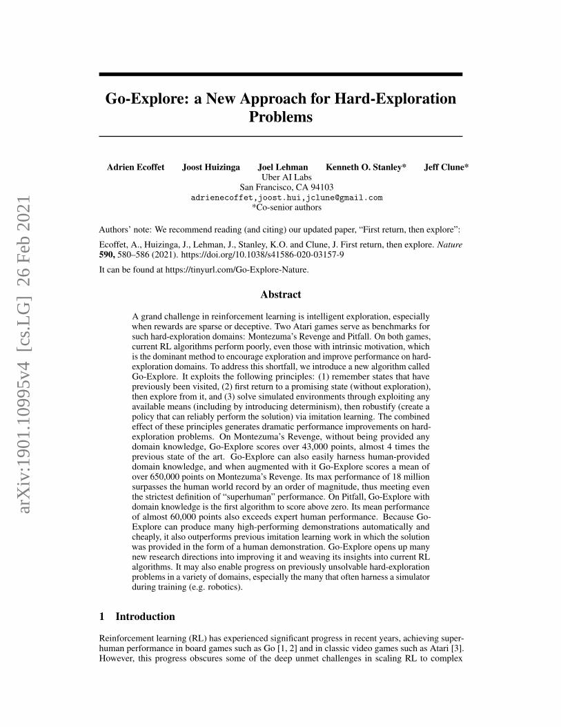
Figure 3: Example cell representation without domain knowledge, which is simply to down-sample each game frame. The full observable state, a color image, is converted to grayscale anddownscaled to an 11× 8 image with 8 possible pixel intensities.

we (1) convert each game frame image to grayscale (2) downscale it to an 11× 8 image with areainterpolation (i.e. using the average pixel value in the area of the downsampled pixel), (3) rescalepixel intensities so that they are integers between 0 and 8, instead of the original 0 to 255 (Fig. 3).The downscaling dimensions and pixel-intensity range were found by grid search. The aggressivedownscaling used by this representation is reminiscent of the Basic feature set from Bellemare et al.[30]. This cell representation requires no game-specific knowledge and is fast to compute.

Cell representations with domain knowledge

The ability of an algorithm to integrate easy-to-provide domain knowledge can be an important asset.In Montezuma’s Revenge, domain knowledge is provided as unique combinations of the x, y positionof the agent (discretized into a grid in which each cell is 16× 16 pixels), room number, level number,and in which rooms the currently-held keys were found. In the case of Pitfall, only the x, y positionof the agent and the room number were used. All this information was extracted directly from pixelswith simple hand-coded classifiers to detect objects such as the main character’s location combinedwith our knowledge of the map structure in the two games (Appendix A.3). While Go-Exploreprovides the opportunity to leverage domain knowledge in the cell representation in Phase 1, therobustified neural network produced by Phase 2 still plays directly from pixels only.

2.1.2 Selecting cells

In each iteration of Phase 1, a cell is chosen from the archive to explore from. This choice could bemade uniformly at random, but we can improve upon that baseline in many cases by creating (orlearning) a heuristic for preferring some cells over others. In preliminary experiments, we foundthat such a heuristic can improve performance over uniform random sampling (data not shown). Theexact heuristic differs depending on the problem being solved, but at a high level, the heuristics in ourwork assign a positive weight to each cell that is higher for cells that are deemed more promising. Forexample, cells might be preferred because they have not been visited often, have recently contributedto discovering a new cell, or are expected to be near undiscovered cells. The weights of all cells arenormalized to represent the probability of each cell being chosen next. No cell is ever given a weightequal to 0, so that all cells in principle remain available for further exploration. The exact heuristicsfrom our experiments are described in Appendix A.5.

2.1.3 Returning to cells and opportunities to exploit deterministic simulators

One of the main principles of Go-Explore is to return to a promising cell without added explorationbefore exploring from that cell. The Go-Explore philosophy is that we should make returning tothat cell as easy as possible given the constraints of the problem. The easiest way to return to acell is if the world is deterministic and resettable, such that one can reset the state of the simulatorto a previous visit to that cell. Whether performing such resets is allowable for RL research is aninteresting subject of debate that was motivated by the initial announcement of Go-Explore [55].The ability to harness determinism and perform such resets forces us to recognize that there are twodifferent types of problems we wish to solve with RL algorithms: those that require stochasticity attest time only, and those that require stochasticity during both testing and training.

We start with the former. Because current RL algorithms can take unsafe actions [56, 57] and requiretremendous amounts of experience to learn [41, 42, 58], the majority of applications of RL in the

6

foreseeable future will likely require training in a simulator before being transferred to (and optionallyfine-tuned in) the real world. For example, most work with learning algorithms for robotics train in asimulator before transferring the solution to the real world; that is because learning directly on therobot is slow, sample-inefficient, can damage the robot, and can be unsafe [59–61]. Fortunately, formany domains, simulators are available (e.g. robotics simulators, traffic simulators, etc.). An insightof Go-Explore is that we can take advantage of the fact that such simulators can be made deterministicto improve performance, especially on hard-exploration problems. For many types of problems, wewant a reliable final solution (e.g. a robot that reliably finds survivors after a natural disaster) andthere is no principled reason to care whether we obtain this solution via initially deterministic training.If we can solve previously unsolvable problems, including ones that are stochastic at evaluation (test)time, via making simulators deterministic, we should take advantage of this opportunity.

There are also cases where a simulator is not available and where learning algorithms must confrontstochasticity during training. To create and test algorithms for this second type of problem, we cannotexploit determinism and resettability. Examples of this class of problems include when we mustlearn directly in the real world (and an effective simulator is not available and cannot be learned),or when studying the learning of biological animals, including ourselves. We believe Go-Explorecan handle such situations by training goal-conditioned policies [62, 63] that reliably return to cellsin the archive during the exploration phase, which is an interesting area for future research. Whilecomputationally much more expensive, this strategy would result in a fully trained policy at the endof the exploration phase, meaning there would be no need for a robustification phase at the end. Wenote that there are some problems where the environment has forms of stochasticity that prevent thealgorithm from reliably returning to a particular cell, regardless of which action the agent takes (e.g.in poker, there is no sequence of actions that reliably leads you to a state where you have two aces).We leave a discussion and study of whether Go-Explore helps in that problem setting for future work.

With this distinction in mind, we can now ask whether Montezuma’s Revenge and Pitfall represent thefirst type of domain (where all we care about is a solution that is robust to stochasticity at test time) orthe second (situations where the algorithm must handle stochasticity while training). We believe fewpeople in the community had considered this question before our initial blog post on Go-Explore [55]and that it created a healthy debate on this subject. Because Atari games are proxies for the problemswe want to solve with RL, and because both types of problems exist, a natural conclusion is that weshould have benchmarks for each. One version of a task can require stochasticity during testing only,and another can require stochasticity during both training and testing. All results and claims in thisversion of this paper are for the version of these domains that does not require stochasticity duringtraining (i.e. stochasticity is required during evaluation only). Applying Go-Explore when training isstochastic remains an exciting avenue of research for the near future.

For problems in which all we care about is a reliable policy at test time, a key insight behindGo-Explore is that we can first solve the problem (Phase 1), and then (if necessary) deal withmaking the solution more robust later (Phase 2). In contrast with the usual view of determinism asa stumbling block to producing agents that are robust and high-performing, it can be made an allyduring exploration and then the solution extended to nondeterminism afterwards via robustification.An important domain where such insights can help is robotics, where training is often done insimulation before policies are transferred to the real world [59–61].

For the experiments in this paper, because we harness deterministic training, we could return to a cellby storing the sequence of actions that lead to it and subsequently replay those actions. However,simply saving the state of the emulator (in addition to this sequence of steps) and restoring that statewhen revisiting a cell gains additional efficiency. Doing so reduced the number of steps that neededto be simulated by at least one order of magnitude (Appendix A.8).

Due to the fact that the present version of Go-Explore operates in a deterministic setting duringPhase 1, each cell is associated with an open-loop sequence of instructions that lead to it given theinitial state, not a proper policy that maps any state to an action. A true policy is produced duringrobustification in Phase 2 (Section 2.2).

2.1.4 Exploration from cells

Once a cell is reached, any exploration method can be applied to find new cells. In this work the agentexplores by taking random actions for k = 100 training frames, with a 95% probability of repeatingthe previous action at each training frame (frames at which the agent is allowed to take an action,

7

thus not including any frames skipped due to frame skip, see Appendix A.1). Besides reaching thek = 100 training frame limit for exploration, exploration is also aborted at the episode’s end (definedin Appendix A.2), and the action that led to the episode ending is ignored because it does not producea destination cell.

Interestingly, such exploration does not require a neural network or other controller, and indeed noneural network was used for the exploration phase (Phase 1) in any of the experiments in this paper(we do not train a neural network until Phase 2). The fact that entirely random exploration works sowell highlights the surprising power of simply returning to promising cells before exploring further,though we believe exploring intelligently (e.g. via a trained policy) would likely improve our resultsand is an interesting avenue for future work.

2.1.5 Updating the archive

While an agent is exploring from a cell, the archive updates in two conditions. The first condition iswhen the agent visits a cell that was not yet in the archive (which can happen multiple times whileexploring from a given cell). In this case, that cell is added to the archive with four associated piecesof metadata: (1) how the agent got to that cell (here, a full trajectory from the starting state to thatcell), (2) the state of the environment at the time of discovering the cell (if the environment supportssuch an operation, which is true for the two Atari-game domains in this paper), (3) the cumulativescore of that trajectory, and (4) the length of that trajectory.

The second condition is when a newly-encountered trajectory is “better” than that belonging to acell already in the archive. For the experiments below, we define a new trajectory as better thanan existing trajectory when the new trajectory either has a higher cumulative score or when it isa shorter trajectory with the same score. In either case, the existing cell in the archive is updatedwith the new trajectory, the new trajectory length, the new environment state, and the new score. Inaddition, information affecting the likelihood of this cell being chosen (see Appendix A.5) is reset,including the total number of times the cell has been chosen and the number of times the cell hasbeen chosen since leading to the discovery of another cell. Resetting these values is beneficial whencells conflate many different states because a new way of reaching a cell may actually be a morepromising stepping stone to explore from (so we want to encourage its selection). We do not reset thecounter that records the number of times the cell has been visited because that would make recentlydiscovered cells indistinguishable from recently updated cells, and recently discovered cells (i.e.those with low visit counts) are more promising to explore because they are likely near the surface ofour expanding sphere of knowledge.

Because cells conflate many states, we cannot assume that a trajectory from start state A through cellB to cell C will still reach C if we substitute a different, better way to get from A to B; therefore,the better way of reaching a cell is not integrated into the trajectories of other cells that built uponthe original trajectory. However, performing such substitutions might work with goal-conditioned orotherwise robust policies, and investigating that possibility is an interesting avenue for future work.

2.1.6 Batch implementation

We implemented Phase 1 in parallel to take advantage of multiple CPUs (our experiments ran on asingle machine with 22 CPU cores): at each step, a batch of b cells is selected (with replacement)according to the rules described in Section 2.1.2 and Appendix A.5, and exploration from each ofthese cells proceeds in parallel for each. Besides using the multiple CPUs to run more instances ofthe environment, a high b also saves time by recomputing cell selection probabilities less frequently,which is important as this computation accounts for a significant portion of run time as the archivegets large (though this latter factor could be mitigated in other ways in the future). Because the sizeof b also has an indirect effect on the exploration behavior of Go-Explore (for instance, the initialstate is guaranteed to be chosen b times at the very first iteration), it is in effect a hyperparameter,whose values are given in Appendix A.6.

2.2 Phase 2: Robustification

If successful, the result of Phase 1 is one or more high-performing trajectories. However, if Phase 1of Go-Explore harnessed determinism in a simulator, such trajectories will not be robust to anystochasticity, which is present at test time. Phase 2 addresses this gap by creating a policy robust to

8

noise via imitation learning, also called learning from demonstration (LfD). Importantly, stochasticityis added during Phase 2 so that the final policy is robust to the stochasticity it will face duringits evaluation in the test environment. Thus the policy being trained has to learn how to mimicand/or perform as well as the trajectory obtained from the Go-Explore exploration phase whilesimultaneously dealing with circumstances that were not present in the original trajectory. Dependingon the stochasticity of the environment, this adjustment can be highly challenging, but nevertheless isfar easier than attempting to solve a sparse-reward problem from scratch.

While most imitation learning algorithms could be used for Phase 2, different types of imitationlearning algorithms can qualitatively affect the resulting policy. LfD algorithms that try to closelymimic the behavior of the demonstration may struggle to improve upon it. For this reason, wechose an LfD algorithm that has been shown capable of improving upon its demonstrations: theBackward Algorithm from Salimans and Chen [28]. It works by starting the agent near the last statein the trajectory, and then running an ordinary RL algorithm from there (in this case Proximal PolicyOptimization (PPO) [64]). Once the algorithm has learned to obtain the same or a higher reward thanthe example trajectory from that starting place near the end of the trajectory, the algorithm backs theagent’s starting point up to a slightly earlier place along the trajectory, and repeats the process untileventually the agent has learned to obtain a score greater than or equal to the example trajectory allthe way from the initial state. Note that a similar algorithm was discovered independently at aroundthe same time by Resnick et al. [65].

While this approach to robustification effectively treats the expert trajectory as a curriculum for theagent, the policy is only optimized to maximize its own score, and not actually forced to accuratelymimic the trajectory. For this reason, this phase is able to further optimize the expert trajectories, aswell as generalize beyond them, both of which we observed in practice in our experiments (Section 3).In addition to seeking a higher score than the original trajectory, because it is an RL algorithm with adiscount factor that prizes near-term rewards more than those gathered later, it also has a pressureto improve the efficiency with which it collects rewards. Thus if the original trajectory containsunnecessary actions (like visiting a dead end and returning), such behavior could be eliminated duringrobustification (a phenomenon we also observed).

2.3 Additional experimental and analysis details

Comparing sample complexity for RL algorithms trained on Atari games can be tricky due to thecommon usage of frame skipping [31, 66], wherein a policy only sees and acts every nth (here, 4)frame, and that action is repeated for intervening frames to save the computation of running the policy.Specifically, it can be ambiguous whether the frames that are skipped are counted (which we call“game frames”) or ignored (which we call “training frames”) when discussing sample complexity. Inthis work, we always qualify the word “frame” accordingly and all numbers we report are measuredin game frames. Appendix A.1 further details the subtleties of this issue.

Because the Atari games are deterministic by default, some form of stochasticity needs to beintroduced to provide a stochastic test environment, which is desirable to make Atari an informativetest bed for RL algorithms. Following previous work, we introduce stochasticity into the Atarienvironment with two previously employed techniques: random no-ops and sticky actions.

Random no-ops means that the agent is forced to take up to 30 no-ops (do nothing commands) at thestart of the game. Because most Atari games run on a timer that affects whether hazards are presentor not, or where different hazards, items, or enemies are located, taking a random number of no-opsputs the world into a slightly different state each time, meaning that fixed trajectories (such as theones found by Go-Explore Phase 1) will no longer work. Random no-ops were first introduced byMnih et al. [3], and they were adopted as a primary source of stochasticity in most subsequent papersworking in the Atari domain [3, 26, 27, 34, 38, 41, 42, 45, 67–73].

While random no-ops prevent single, memorized trajectories from solving Atari games, the remainderof the game remains deterministic, meaning there is still much determinism that can be exploited.While several other forms of stochasticity have been proposed (e.g. humans restarts [74], randomframe skips [75], etc.), a particularly elegant form is sticky actions [31], where at each game framethere exists some probability of repeating the previous action instead of performing a newly chosenaction. This way to introduce stochasticity is akin to how humans are not frame perfect, but may holda button for slightly longer than they intended, or how they may be slightly late in pressing a button.

9

Because Atari games have been designed for human play, the addition of sticky actions generallydoes not prevent a game from being solvable, and it adds some stochasticity to every state in thegame, not just the start. Although our initial blog post [55] only included random no-ops, in thispaper our robustification and all post-robustification test results are produced with a combinationof both random no-ops and sticky actions. All algorithms we compare against in Section 3 and inAppendix A.9 likewise were tested with some form of stochasticity (in the form of no-ops, stickyactions, human starts, or some combination thereof), though it is worth noting that, unlike Go-Explore,most also had to handle stochasticity throughout training. Relevant algorithms that were tested in adeterministic environment are discussed in Section 5.

All hyperparameters were found by performing a separate grid-search for each experiment. Thefinal, best performing hyperparameters are listed in Appendix A.6, tables 1 and 2. All confidenceintervals given are 95% bootstrapped confidence intervals computed using the pivotal (also known asempirical) method [76], obtained by resampling 10,000 times. Confidence intervals are reported withthe following notation: stat (CI: lower – upper) where stat is the statistic (a mean unless otherwisespecified). In graphs containing shaded areas, those areas indicate the 95% percentile bootstrappedconfidence interval of the mean, obtained by resampling 1,000 times. Graphs of the exploration phase(Phase 1) depict data at approximately every 4M game frames and graphs of the robustification phase(Phase 2) depict data at approximately every 130,000 game frames.

Because the robustification process can diverge even after finding a solution, the neural networkat the end of training does not necessarily perform well, even if a high-performing solution wasfound at some point during this process. To retrieve a neural network that performs well regard-less of when it was found, all robustification runs (Phase 2) produced a checkpoint of the neuralnetwork approximately every 13M game frames. Because the performance values recorded duringrobustification are noisy, we cannot select the best performing checkpoint from those performancevalues alone. As such, at the end of each robustification run, out of the checkpoints with the lowestmax_starting_point (or close to it), a random subset of checkpoints (between 10 and 50) wastested to evaluate the performance of the neural network stored within that checkpoint. We test arandom subset because robustification runs usually produce more successful checkpoints then we canrealistically test. The highest-scoring checkpoint for each run was then re-tested to account for theselection bias inherent in selecting the best checkpoint. The scores from this final retest are the oneswe report.

The neural network from each checkpoint is evaluated with random no-ops and sticky actions until atleast 5 scores for each of the 31 possible starting no-ops (from 0 to 30 inclusive) are obtained. Themean score for each no-op is then calculated and the final score for the checkpoint is the grand meanof the individual no-op scores. Unless otherwise specified, the default time limit of 400,000 gameframes imposed by OpenAI Gym [75] is enforced.

3 Results

3.1 Montezuma’s Revenge

3.1.1 Without domain knowledge in the cell representation

In this first experiment, we run Go-Explore on Montezuma’s Revenge with the downsampled imagecell representation, which does not require game-specific domain knowledge. Despite the simplicityof this cell representation, Phase 1 of Go-Explore solves level 1 in 57% of runs after 1.2B gameframes (a modest number by modern standards [41, 42]), with one of the 100 runs also solving level2, and visits a mean of 35 rooms (CI: 33 – 37) (Fig. 4a). The number of new cells being discovered isstill increasing linearly after 1.2B game frames, indicating that results would likely be even betterwere it run longer (Fig. 4b). Phase 1 of Go-Explore achieves a mean score of 57,439 (CI: 47,843 –67,224) (Fig. 4c). Level 1 was solved after a mean of 640M (CI: 567M – 711M) game frames, whichtook a mean of 10.8 (CI: 9.5 – 12.0) hours on a single, 22-CPU machine (note that these level 1numbers exclude the runs that never solved level 1 after 1.2B game frames). See Appendix A.8 formore details on performance.

Amusingly, Go-Explore discovered a little-known bug in Montezuma’s Revenge called the “treasureroom curse” [77]. If the agent performs a specific sequence of actions, it can remain in the treasureroom (the final room before being sent to the next level) indefinitely, instead of being automatically

10

0.0 0.5 1.0Game Frames 1e9

0

10

20

30

Foun

d Ro

oms

State of the art

(a) Number of rooms found

0.0 0.5 1.0Game Frames 1e9

0

5,000

10,000

15,000

Foun

d Ce

lls

(b) Number of cells found

0.0 0.5 1.0Game Frames 1e9

0

20,000

40,000

60,000

Best

Sco

re

Average Human

Human Expert

(c) Maximum score in archive

Figure 4: Performance of the exploration phase of Go-Explore with downscaled frames onMontezuma’s Revenge. Lines indicating human and the algorithmic state of the art are for compar-ison, but recall that the Go-Explore scores in this plot are on a deterministic version of the game(unlike the post-Phase 2 scores presented in this section).

0.0 0.2 0.4 0.6 0.8 1.0 1.2 1.4 1.6Game Frames 1e9

0

1,000

2,000

3,000

4,000

5,000

Max

Sta

rting

Poi

nt

(a) Failed robustification with 1 demonstration

0.0 0.2 0.4 0.6 0.8 1.0 1.2 1.4 1.6Game Frames 1e9

0

5,000

10,000

15,000

20,000

25,000

30,000

Max

Sta

rting

Poi

nt

Demo 0Demo 1Demo 2Demo 3Demo 4Demo 5Demo 6Demo 7Demo 8Demo 9

(b) Successful robustification with 10 demonstrations

Figure 5: Examples of maximum starting point over training for robustifying using differentnumbers of demonstrations. Success is achieved as soon as any of the curves gets sufficiently close(e.g. within 50 units) to 0, because that means the agent is able to perform as well as at least one ofthe demonstrations.

moved to the next level after some time. Because gems giving 1,000 points keep appearing in thetreasure room, it is possible to easily achieve very high scores once it has been triggered. Finding bugsin games and simulators, as Go-Explore did, is an interesting reminder of the power and creativity ofoptimization algorithms [6], and is commercially valuable as a debugging tool to identify and fix suchbugs before shipping simulators and video games. A video of the treasure room curse as triggered byGo-Explore is available at https://youtu.be/civ6OOLoR-I.

In 51 out of the 57 runs that solved level 1, the highest-scoring trajectory found by Go-Exploreexploited the bug. To prevent scores from being inflated due to this bug, we filtered out trajectoriesthat triggered the treasure room curse bug when extracting the highest scoring trajectory from eachrun of Go-Explore for robustification (Appendix A.4 provides details).

As mentioned in Section 2.2, we used Salimans & Chen’s Backward Algorithm [28] for robustification.However, we found it somewhat unreliable in learning from a single demonstration (Fig. 5a). Indeed,only 40% of our attempts at robustifying trajectories that solved level 1 were successful when using asingle demonstration.

However, because Go-Explore can produce many demonstrations, we modified the Backward Algo-rithm to simultaneously learn from multiple demonstrations (details in Appendix A.7). To simulatethe use case in which Phase 1 is run repeatedly until enough successful demonstrations (in this case10) are found, we extracted the highest scoring non-bug demonstration from each of the 57 out of

11

2013 2014 2015 2016 2017 2018 2019Time of publication

0

10,000

20,000

30,000

40,000

Scor

e

Avg. Human

Human Expert

SARSALinear DQN

GorilaMP-EB

DDQN

Duel. DQNPrior. DQN

A3CPop-Art

A3C-CTSDQN-CTS

BASS-hashES

DQN-PixelCNNReactor

Feature-EB

C51

UBE

Rainbow

IMPALAApe-X

RNDPPO+CoEX

Go-Explore

Figure 6: History of progress on Montezuma’s Revenge vs. the version of Go-Explore that doesnot harness domain knowledge. Go-Explore significantly improves on the prior state of the art.These data are presented in tabular form in Appendix A.9.

100 Phase 1 runs that had solved level 1, and randomly assigned them to one of 5 non-overlappinggroups of 10 demonstrations (7 demonstrations were left over and ignored), each of which was usedfor a robustification run. When training with 10 demonstration trajectories, all 5 robustification runswere successful. Fig. 5b shows an example of successful robustification with 10 trajectories.

In the end, our robustified policies achieve a mean score of 43,763 (CI: 36,718 – 50,196), substantiallyhigher than the human expert mean of 34,900 [27]. All policies successfully solve level 1 (with a99.8% success rate over different stochastic evaluations of the policies), and one of our 5 policiesalso solves level 2 100% of the time. Fig. 6 shows how these results compare with prior work.

Surprisingly, the computational cost of Phase 2 is greater than that of Phase 1. These Phase 2 resultswere achieved after a mean of 4.35B (CI: 4.27B – 4.45B) game frames of training, which took amean of 2.4 (CI: 2.4 – 2.5) days of training (details in Appendix A.8).

3.1.2 With domain knowledge in the cell representation

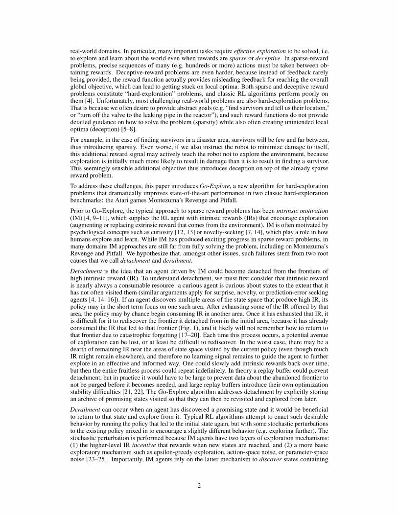
On Montezuma’s Revenge, when harnessing domain knowledge in its cell representation (Sec-tion 2.1.1), Phase 1 of Go-Explore finds a total of 238 (CI: 231 – 245) rooms, solves a mean of 9.1(CI: 8.8 – 9.4) levels (with every run solving at least 7 levels), and does so in roughly half as manygame frames as with the downscaled image cell representation (Fig. 7a). Its scores are also extremelyhigh, with a mean of 148,220 (CI: 144,580 – 151,730) (Fig. 7c). These results are averaged over 50runs.

As with the downscaled version, Phase 1 of Go-Explore with domain knowledge was still discoveringadditional rooms, cells, and ever-higher scores linearly when it was stopped (Fig. 7). Indeed, becauseevery level of Montezuma’s Revenge past level 3 is nearly identical to level 3 (except for the scoreson the screen and the stochastic timing of events) and because each run had already passed level 3, itwould likely continue to find new rooms, cells, and higher scores forever.

Domain knowledge runs spend less time exploiting the treasure room bug because we preferentiallyselect cells in the highest level reached so far (Appendix A.5). Doing so encourages exploring newlevels instead of exploring the treasure rooms on previous levels to keep exploiting the treasure roombug. The highest final scores thus come from trajectories that solved many levels. Because knowingthe level number constitutes domain knowledge, non-domain knowledge runs cannot take advantageof this information and are thus affected by the bug more.

12

0.0 0.5 1.0Game Frames 1e9

0

50

100

150

200

250

Foun

d Ro

oms

State of the art

Go-Explore(no domainknowledge)Go-Explore(domainknowledge)

(a) Number of rooms found

0.0 0.5 1.0Game Frames 1e9

0

10,000

20,000

30,000

40,000

50,000

Foun

d Do

mai

n Kn

owle

dge

Cells

(b) Number of cells found

0.0 0.5 1.0Game Frames 1e9

0

25,000

50,000

75,000

100,000

125,000

150,000

Best

Sco

re

Average Human

Human Expert

(c) Maximum score in archive

Figure 7: Performance on Montezuma’s Revenge of Phase 1 of Go-Explore with and withoutdomain knowledge. The algorithm finds more rooms, cells, and higher scores with the easilyprovided domain knowledge, and does so with a better sample complexity. For (b), we plot thenumber of cells found in the no-domain-knowledge runs according to the more intelligent cellrepresentation from the domain-knowledge run to allow for an equal comparison.

In terms of computational performance, Phase 1 with domain knowledge solves the first level aftera mean of only 57.6M (CI: 52.7M – 62.3M) game frames, corresponding to 0.9 (CI: 0.8 – 1.0)hours on a single 22-CPU machine. Solving level 3, which effectively means solving the entiregame as discussed above, is accomplished in a mean of 173M (CI: 164M – 182M) game frames,corresponding to 6.8 (CI: 6.2 – 7.3) hours. Appendix A.8 provides full performance details.

For robustification, we chose trajectories that solve level 3, truncated to the exact point at which level3 is solved because, as mentioned earlier, all levels beyond level 3 are nearly identical aside from thepixels that display the score, which of course keep changing, and some global counters that changethe timing of aspects of the game like when laser beams turn on and off.

We performed 5 robustification runs with demonstrations from the Phase 1 experiments above, eachof which had a demonstration from each of 10 different Phase 1 runs. All 5 runs succeeded. Theresulting mean score is 666,474 (CI: 461,016 – 915,557), far above both the prior state of the art andthe non-domain knowledge version of Go-Explore. As with the downscaled frame version, Phase 2was slower than Phase 1, taking a mean of 4.59B (CI: 3.09B – 5.91B) game frames, corresponding toa mean of 2.6 (CI: 1.8 – 3.3) days of training.

The networks show substantial evidence of generalization to the minor changes in the game beyondlevel 3: although the trajectories they were trained on only solve level 3, these networks solved amean of 49.7 levels (CI: 32.6 – 68.8). In many cases, the agents did not die, but were stopped bythe maximum limit of 400,000 game frames imposed by default in OpenAI Gym [75]. Removingthis limit altogether, our best single run from a robustified agent achieved a score of 18,003,200 andsolved 1,441 levels during 6,198,985 game frames, corresponding to 28.7 hours of game play (at60 game frames per second, Atari’s original speed) before losing all its lives. This score is over anorder of magnitude higher than the human world record of 1,219,200 [78], thus achieving the strictestdefinition of “superhuman” performance. A video of the agent solving the first ten levels can be seenhere: https://youtu.be/gnGyUPd_4Eo.

Fig. 8 compares the performance of Go-Explore to historical results (including the previous state ofthe art), the no-domain-knowledge version of Go-Explore, and previous imitation learning work thatrelied on human demonstrations to solve the game. The version of Go-Explore that harnesses domainknowledge dramatically outperforms them all. Specifically, Go-Explore produces scores over 9 timesgreater than those reported for imitation learning from human demonstrations [28] and over 55 timesthe score reported for the prior state of the art without human demonstrations [39].

That Go-Explore outperforms imitation learning plus human demonstrations is particularly notewor-thy, as human-provided solutions are arguably a much stronger form of domain knowledge than thatprovided to Go-Explore. We believe that this result is due to the higher quality of demonstrationsthat Go-Explore was able to produce for Montezuma’s Revenge vs. those provided by humans in theprevious imitation learning work. The demonstrations used in our work range in score from 35,200to 51,900 (lower than the final mean score of 148,220 for Phase 1 because these demonstrations are

13

2013 2014 2015 2016 2017 2018 2019Time of publication

0

100,000

200,000

300,000

400,000

500,000

600,000

Scor

e

Human ExpertSARSALinear DQN

GorilaMP-EB

DDQN

Duel. DQN

A3CA3C-CTS

DQN-CTS

BASS-hash

DQN-PixelCNNDQfD

UBEApe-X

Ape-X DQfD TDC+CMC

DeepCS

LfSD (best)

RNDPPO+CoEX

Go-Explore (domain knowledge)

Go-Explore

No Domain KnowledgeHuman DemonstrationDomain Knowledge

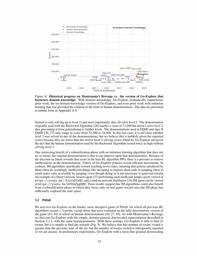
Figure 8: Historical progress on Montezuma’s Revenge vs. the version of Go-Explore thatharnesses domain knowledge. With domain knowledge, Go-Explore dramatically outperformsprior work, the no-domain-knowledge version of Go-Explore, and even prior work with imitationlearning that was provided the solution in the form of human demonstrations. The data are presentedin tabular form in Appendix A.9.

limited to only solving up to level 3) and most importantly, they all solve level 3. The demonstrationoriginally used with the Backward Algorithm [28] reaches a score of 71,500 but doesn’t solve level 3,thus preventing it from generalizing to further levels. The demonstrations used in DQfD and Ape-XDQfD [26, 27] only range in score from 32,300 to 34,900. In this last case, it is not clear whetherlevel 3 was solved in any of the demonstrations, but we believe this is unlikely given the reportedscores because they are lower than the lowest level-3-solving scores found by Go-Explore and giventhe fact that the human demonstration used by the Backward Algorithm scored twice as high withoutsolving level 3.

One interesting benefit of a robustification phase with an imitation learning algorithm that does nottry to mimic the original demonstration is that it can improve upon that demonstration. Because ofthe discount on future rewards that exists in the base RL algorithm PPO, there is a pressure to removeinefficiencies in the demonstration. Videos of Go-Explore policies reveal efficient movements. Incontrast, IM algorithms specifically reward reaching novel states, meaning that policies produced bythem often do seemingly inefficient things like deviating to explore dead ends or jumping often totouch states only accessible by jumping, even though doing so is not necessary to gain real reward.An example of a Deep Curiosity Search agent [37] performing such inefficient jumps can be viewed athttps://youtu.be/-Fy2va3IbQU, and a random network distillation [16] IM agent can be viewedat https://youtu.be/40VZeFppDEM. These results suggest that IM algorithms could also benefitfrom a robustification phase in which they focus only on real-game reward once the IM phase hassufficiently explored the state space.

3.2 Pitfall

We next test Go-Explore on the harder, more deceptive game of Pitfall, for which all previous RLalgorithms scored ≤ 0 points, except those that were evaluated on the fully deterministic version ofthe game [43, 44] or relied on human demonstrations [26, 27, 45]. As with Montezuma’s Revenge,we first run Go-Explore with the simple, domain-general, downscaled representation described inSection 2.1.1, with the same hyperparameters. With these settings, Go-Explore is able to find 22rooms, but it is unable to find any rewards (Fig. 9). We believe that this number of rooms visited isgreater than the previous state of the art, but the number of rooms visited is infrequently reportedso we are unsure. In preliminary experiments, Go-Explore with a more fine-grained downscaling

14

0 1 2 3 4Game Frames 1e9

0

50

100

150

200

250

Foun

d Ro

oms Go-Explore

(no domainknowledge)Go-Explore(domainknowledge)

(a) Number of rooms found

0 1 2 3 4Game Frames 1e9

0

2,500

5,000

7,500

10,000

12,500

15,000

Foun

d Do

mai

n Kn

owle

dge

Cells

(b) Number of cells found

0 1 2 3 4Game Frames 1e9

0

20,000

40,000

60,000

Best

Sco

re

Average Human

Human Expert

(c) Maximum score in archive

Figure 9: Performance on Pitfall of Phase 1 of Go-Explore with and without domain knowledge.Without domain knowledge, the exploration phase finds about 22 rooms (a), but it then quickly stopsfinding new rooms (a) or cells (b) (here, we display discovery of domain-knowledge cells to enable afair comparison, see Appendix A.10 for progress on the domain-agnostic cell representation), and itdoesn’t find any rewards (c). With domain knowledge, the exploration phase of Go-Explore finds all255 rooms (a) and trajectories scoring a mean 70,264 points (c). In addition, even though the numberof rooms (a) and the number cells (b) found stagnates after about 2B game frames, score continues togo up for about another billion game frames. This is possible because, in Pitfall, there can exist manydifferent trajectories to the same cell that vary in score. As such, once all reachable cells have beendiscovered, Go-Explore relies on replacing lower-scoring trajectories with higher-scoring trajectoriesto increase its score. The final score is not the maximum score that can be reached in Pitfall (themaximum score in Pitfall is 112,000), but Go-Explore finds itself in a local optima where higherscoring trajectories cannot be found starting from any of the trajectories currently in the archive.Lines represent the mean over 10 (without domain knowledge) and 40 (with domain knowledge)independent runs.

procedure (assigning 16 different pixel values to the screen, rather than just 8) is able to find up to 30rooms, but it then runs out of memory (Appendix A.10). Perhaps with a more efficient or distributedcomputational setup this representation could perform well on the domain, a subject we leave tofuture work. We did not attempt to robustify any of the trajectories because no positive reward wasfound.

We believe the downscaled-image cell representation underperforms on Pitfall because the game ispartially observable, and frequently contains many importantly different states that appear almostidentical (even in the unaltered observation space of the game itself), but require different actions(Appendix A.12). One potential solution to this problem would be to change to a cell representationthat takes previous states into account to disambiguate such situations. Doing so is an interestingdirection for future work.

Next, we tested Go-Explore with domain knowledge (Section 2.1.1). The cell representation withdomain knowledge is not affected by the partial observability of Pitfall because it maintains the roomnumber, which is information that disambiguates the visually identical states (note that we can keeptrack of the room number from pixel information only by keeping track of all screen transitions thathappened along the trajectory). With it, the exploration phase of Go-Explore (Phase 1) is able to visitall 255 rooms and its best trajectories collect a mean of 70,264 (CI: 67,287 – 73,150) points (Fig. 9).

We attempted to robustify the best trajectories, but the full-length trajectories found in the explorationphase did not robustify successfully (Appendix A.11), possibly because different behaviors maybe required for states that are visually hard to distinguish (Appendix A.12). Note that the domain-knowledge cell representation does not help in this situation, because the network trained in therobustification phase (Phase 2) is not presented with the cell representation from the exploration phase(Phase 1). The network thus has to learn to keep track of past information by itself. Rememberingthe past is possible, as the network of the agent does include a fully recurrent layer, but it is unclearto what degree this layer stores information from previous rooms, especially because the BackwardAlgorithm loads the agent at various points in the game without providing the agent with the historyof rooms that came before. This can make it difficult for the agent to learn to store information fromprevious states. As such, robustifying these long trajectories remains a topic for future research.

15

2015 2016 2017 2018 2019Time of publication

0

10,000

20,000

30,000

40,000

50,000

60,000

Scor

e

Avg. Human

Expert Human

DQN DDQN

Duel. DQN

Prior. DQN

A3C Pop-ArtA3C-CTS

DQN-CTS

C51UBE

Rainbow IMPALADQN-

PixelCNN

Reactor

Ape-X RNDDeepCS

Go-ExploreDomain KnowledgeNo Domain Knowledge

Figure 10: Historical progress on Pitfall vs. the version of Go-Explore that harnesses domainknowledge. Go-Explore achieves a mean of over 59,000 points, greatly outperforming the prior stateof the art. The data are presented in tabular form in Appendix A.9.

We found that shorter trajectories scoring roughly 35,824 (CI: 34,225 – 37,437) points could besuccessfully robustified. To obtain these shorter trajectories, we truncated all trajectories in thearchive produced in Phase 1 to 9,000 training frames (down from the total of 18,000 training frames),and then selected the highest scoring trajectory out of these truncated trajectories. We then furthertruncated this highest scoring trajectory such that it would end right after the collection of the lastobtained reward, to ensure that the Backward Algorithm would always start right before obtaining areward, resulting in trajectories with a mean length of 8,304 (CI: 8,118 – 8,507) training frames.

From the truncated trajectories, the robustification phase (Phase 2) of Go-Explore is able to produceagents that collect 59,494 (CI: 49,042 – 72,721) points (mean over 10 independent runs), substantiallyoutperforming both the prior state of the art and human experts (Fig. 10). These trajectories requireda mean of 8.20B (CI: 6.73B – 9.74B) game frames to robustify, which took a mean of 4.5 (CI: 3.7 –5.3) days. The best rollout of the best robustified policy obtained a score of 107,363 points, and avideo of this rollout is available at: https://youtu.be/IJMdYOnsDpA.

Interestingly, the mean performance of the robustified networks of 59,494 is higher than the maximumperformance among the demonstration trajectories of 45,643. This score difference is too large to bethe result of small optimizations along the example trajectories (e.g. by avoiding more of the negativerewards in the environment), thus suggesting that, as with Montezuma’s Revenge, these policies areable to generalize well beyond the example trajectories they were provided.

4 Discussion and Future Work

Three key principles enable Go-Explore to perform so well on hard-exploration problems: (1) re-member good exploration stepping stones, (2) first return to a state, then explore and, (3) first solve aproblem, then robustify (if necessary).

These principles do not exist in most RL algorithms, but it would be interesting to weave them in.As discussed in Section 1, contemporary RL algorithms do not do follow principle 1, leading todetachment. Number 2 is important because current RL algorithms explore by randomly perturbingthe parameters or actions of the current policy in the hope of exploring new areas of the environment,which is ineffective when most changes break or substantially change a policy such that it cannotfirst return to hard-to-reach states before further exploring from them (an issue we call derailment).Go-Explore solves this problem by first returning to a state and then exploring from there. Doing so

16

enables deep exploration that can find a solution to the problem, which can then be robustified toproduce a reliable policy (principle number 3).

The idea of preserving and exploring from stepping stones in an archive comes from the qualitydiversity (QD) family of algorithms (like MAP-elites [60, 79] and novelty search with local competi-tion [80]), and Go-Explore is an enhanced QD algorithm based on MAP-Elites. However, previousQD algorithms focus on exploring the space of behaviors by randomly perturbing the current archiveof policies (in effect departing from a stepping stone in policy space rather than in state space), asopposed to explicitly exploring state space by departing to explore anew from precisely where in statespace a previous exploration left off. In effect, Go-Explore offers significantly more controlled explo-ration of state space than other QD methods by ensuring that the scope of exploration is cumulativethrough state space as each new exploratory trajectory departs from the endpoint of a previous one.

It is remarkable that the current version of Go-Explore works by taking entirely random actions duringexploration (without any neural network) and that it is effective even when applied on a very simplediscretization of the state space. Its success despite such surprisingly simplistic exploration stronglysuggests that remembering and exploring from good stepping stones is a key to effective exploration,and that doing so even with otherwise naive exploration helps the search more than contemporarydeep RL methods for finding new states and representing those states. Go-Explore might be madeeven more powerful by combining it with effective, learned representations. It could further benefitfrom replacing the current random exploration with more intelligent exploration policies, whichwould allow the efficient reuse of skills required for exploration (e.g. walking). Both of these possibleimprovements are promising avenues for future work.

Go-Explore also demonstrates how exploration and dealing with environmental stochasticity areproblems that can be solved separately by first performing exploration in a deterministic environmentand then robustifying relevant solutions. The reliance on having access to a deterministic environmentmay initially seem like a drawback of Go-Explore, but we emphasize that deterministic environmentsare available in many popular RL domains, including videos games, robotic simulators, or evenlearned world models. Once a brittle solution is found, or especially a diverse set of brittle solutions,a robust solution can then be produced in simulation. If the ultimate goal is a policy for the realworld (e.g. in robotics), one can then use any of the many available techniques for transferring therobust policy from simulation to the real world [59, 60, 81]. In addition, we expect that future workwill demonstrate that it is possible to substitute exploiting determinism to return to states with agoal-conditioned policy [62, 63] that learns to deal with stochastic environments from the start (duringtraining). Such an algorithm would still benefit from the first two principles of Go-Explore, andpossibly the third too, as even a goal-conditioned policy could benefit from additional optimizationonce the desired goal is known.

A possible objection is that, while this method already works in the high-dimensional domain ofAtari-from-pixels, it might not scale to truly high-dimensional domains like simulations of the realworld. We believe Go-Explore can be adapted to such high-dimensional domains, but it will likelyhave to marry a more intelligent cell representation of interestingly different states (e.g. learned,compressed representations of the world) with intelligent (instead of random) exploration. Indeed,the more conflation (mapping more states to the same cell) one does, the more probable it is that onewill need intelligent exploration to reach such qualitatively different cells.

Though our current implementation of Go-Explore can handle the deceptive reward structure foundin Pitfall, its exploitation of determinism makes it vulnerable to a new form of deception we call the“busy-highway problem.” Consider an environment in which the agent needs to cross a busy highway.One option is to traverse the highway directly on foot, but that creates so much risk of being hit by acar that no policy could reliably cross this way. A safer alternative would be to take a bridge thatgoes over the highway, which would constitute a detour, but be guaranteed to succeed. By making theenvironment deterministic for Phase 1, the current version of Go-Explore would eventually succeed intraversing the highway directly, leading to a much shorter trajectory than by taking the bridge. Thusall the solutions chosen for robustification will be ones that involve crossing the highway directlyinstead of taking the bridge, making robustification impossible.

One solution to this issue would be to provide robustification with more demonstrations from Phase 1of Go-Explore (which could include some that take the bridge instead of crossing the highway), oreven all of the trajectories it gathers during Phase 1. With this approach, robustification would beable to fall back on the bridge trajectories when the highway trajectories fail to robustify. While this

17

approach should help, it may still be the case that so much of the experience gathered by Go-ExplorePhase 1 is dependent on trajectories that are impossible to reproduce reliably that learning fromthese Go-Explore trajectories is less efficient than learning from scratch. How common this class ofproblem is in practice is an empirical question and an interesting subject for future work. However,we hypothesize that versions of Go-Explore that deal with stochasticity throughout training (e.g. bytraining goal-conditioned policies to return to states) would not be affected by this issue, as theywould not succeed in crossing the highway reliably except by taking the bridge.

One promising area for future work is robotics. Many problems in robotics, such as figuring out theright way to grasp an object, how to open doors, or how to locomote, are hard-exploration problems.Even harder are tasks that require long sequences of actions, such as asking a robot to find survivors,clean a house, or get a drink from the refrigerator. Go-Explore could enable a robot to learn how todo these things in simulation. Because conducting learning in the real world is slow and may damagethe robot, most robotic work already involves first optimizing in a simulator and then transferring thepolicy to the real world [59–61, 82]. Go-Explore’s ability to exploit determinism can then be helpfulbecause robotic simulators could be made deterministic for Phase 1 of Go-Explore. The full pipelinecould look like the following: (1) Solve the problem in a deterministic simulator via Phase 1 ofGo-Explore. (2) Robustify the policy in simulation by adding stochasticity to the simulation via Phase2 of Go-Explore. (3) Transfer the policies to the real world, optionally adding techniques to helpcross the simulation-reality gap [59–61], including optionally further learning via these techniques orany learning algorithm. Of course, this pipeline could also be changed to using a goal-conditionedversion of Go-Explore if appropriate. Overall, we are optimistic that Go-Explore may make manypreviously unsolvable robotics problems solvable, and we are excited to see future research in thisarea from our group and others.

Interestingly, the Go-Explore algorithm has implications and applications beyond solving sparse- ordeceptive-reward problems. The algorithm’s ability to broadly explore the state space can unearthimportant facets of the domain that go beyond reward, e.g. the distribution of states that contain aparticular agent (e.g. a game character or robot) or are near to catastrophic outcomes. For example,within AI safety [5] one open problem is that of safe exploration [83], wherein the process of trainingan effective real-world policy is constrained by avoiding catastrophe-causing actions during thattraining. In the robotics setting where Go-Explore is applied in simulation (before attempting transferto the real world), the algorithm could be driven explicitly to search for diverse simulated catastrophes(in addition to or instead of reward). Such a catastrophe collection could then be leveraged to trainagents that act more carefully in the real world, especially while learning [84, 85]. Beyond thisexample, there are likely many other possibilities for how the data produced by Go-Explore could beproductively put to use (e.g. as a source of data for generative models, to create auxiliary objectivesfor policy training, or for understanding other agents in the environment by inverse reinforcementlearning).

5 Related Work

Go-Explore is reminiscent of earlier work that separates exploration and exploitation (e.g. Colas et al.[86]), in which exploration follows a reward-agnostic Goal Exploration Process [87] (an algorithmsimilar to novelty search [7]), from which experience is collected to prefill the replay buffer of anoff-policy RL algorithm, in this case DDPG [88]. This algorithm then extracts the highest-rewardingpolicy from the experience gathered. In contrast, Go-Explore further decomposes exploration intothree elements: Accumulate stepping stones (interestingly different states), return to promisingstepping stones, and explore from them in search of additional stepping stones (i.e. principles 1 and 2above). The impressive results Go-Explore achieves by slotting in very simple algorithms for eachelement shows the value of this decomposition.

The aspect of Go-Explore of first finding a solution and then robustifying around it has precedent inGuided Policy Search [89]. However, this method requires a non-deceptive, non-sparse, differentiableloss function to find solutions, meaning it cannot be applied directly to problems where rewardsare discrete, sparse, or deceptive, as both Atari and many real-world problems are. Further, GuidedPolicy Search requires having a differentiable model of the world or learning a set of local models,which to be tractable requires the full state of the system to be observable during training time.

18

More recently, Oh et al. [90] combined A2C with a “Self-Imitation Learning” loss on the best trajec-tories found during training. This is reminiscent of Go-Explore’s robustification phase, except for thefact that Self-Imitation Learning’s imitation loss is used throughout learning, while imitation learningis a separate phase in Go-Explore. Self-Imitation Learning’s 2,500 point score on Montezuma’sRevenge was close to the state of the art at the time of its publication.

Another algorithm that is related to the idea of first returning before exploring is BootstrappedDQN [91]. It trains an ensemble of networks that approximate the Q function, but with bootstrappingthe data so each network is trained on a different random subset of the data. Each training episode, itpicks one of the networks and acts according to the policy it implies. In frequently visited areas of thesearch space, all of the networks will have lots of data and are likely to converge to the same policy(thus, exploration will be low). However, in rarely visited areas of the state space, the networks wouldideally have different Q-value predictions, meaning that in different episodes different choices will bemade, yielding exploration. At a high level, the dynamics can thus allow an agent to first return to anarea of the search space with little exploration before exploring from it. That said, this algorithm willstill try to focus on returning to one narrow area of the search space (the one it is currently exploring,see the flashlight metaphor of IM algorithms in Section 1) before exploring, and thus is still likely tosuffer from the issue of detachment described in Section 1. Indeed, empirically Bootstrapped DQNscores only 100 on Montezuma’s Revenge, and detachment may be a large reason why.

Recall Traces [92] also implement the idea of returning to previously discovered states. They do soby running a backtracking model to create virtual trajectories towards states heuristically consideredvaluable and they include those virtual trajectories during training with the help of an imitationlearning loss, thereby increasing the likelihood that these states will be revisited and explored from.Contrary to Go-Explore, Recall Traces do not separate returning to states and exploring from thosestates, thus the algorithm helps ameliorate detachment, but not derailment. The method improvedsample efficiency in several sparse reward domains, but was not tested on Montezuma’s Revenge orPitfall.

Closely related to the first two principles of Go-Explore is the work by Liu et al. [43], which takesa hierarchical reinforcement learning approach in which an abstract MDP is created through theconflation of multiple states into abstract states, which are similar to the cells in Go-Explore. Thisabstract MDP stores all abstract states (i.e. cells) that it encounters, thus keeping track of promisingstates to explore from, and it navigates the MDP in a reliable way before exploring from a selectedabstract-MDP state, thus implementing the idea of returning before exploring. One difference withGo-Explore is that this algorithm does not use a trajectory of actions to return to a cell, but insteadrelies on a set of sub-policies, called skills, which are executed in sequence to navigate the abstractMDP. While this set of skills is flexible, in that it allows the same skill to be reused for differenttransitions, it takes time to train a new skill, potentially making it computationally expensive toexplore as deep into the game as Go-Explore does. Another difference is that the algorithm by Liuet al. [43] does not implement a robustification phase, but instead relies on the abstract MDP, evenat evaluation time. While this means the algorithm does not require any additional training, it alsomeans the algorithm can never improve upon the limits of the constructed MDP. The algorithmfrom Liu et al. [43], which harnesses domain knowledge, scores 12,500 on Montezuma’s Revengeand 15,000 on Pitfall, though these scores come from evaluation in the deterministic version of theenvironment (they do provide results on stochastic test environments for a different game: PrivateEye). Go-Explore scores substantially more in both Montezuma’s Revenge and Pitfall despite beingtested in a stochastic environment and, in the case of Montezuma’s Revenge, even when not relyingon domain knowledge.

In a similar vein, Dong et al. [93] maintains an explicit memory of novel states and explores afterreturning to them via a goal-conditioned policy, though their algorithm only reaches scores of around1,000 on Montezuma’s Revenge, substantially less than Go-Explore. We speculate that this is due to(1) Its use of a fixed-capacity pool of potential next states to visit, which might not be able to keep upwith the large number of possible interestingly different states present in Montezuma’s Revenge, and(2) By determining whether a goal is reached based on a pixel based measure, their goal-conditionedpolicy could have a hard time learning to return to a previously visited state, as the pixel-basedmatch requires all moving objects, such as enemies, to be in very similar locations before a goal isconsidered reached. The insights of keeping an archive of known states and exploring to discovernew states to add to the archive dates back at least to the E3 algorithm [94], although the E3 authorsnote that it does not work in high-dimensional problems for which tabular methods are intractable

19

and function approximation (or some form of conflation) is required. Go-Explore can be seen as anE3-like algorithm that adapts some of its principles to high-dimensional domains.

The idea of planning (searching in a deterministic model of the world to find a good strategy) and thentraining a policy to mimic what was learned is reminiscent of Guo et al. [95]. It plans (in the Atariemulator) with UCT [47–49], which is slow, and then trains a much faster policy with supervisedlearning to imitate the planning algorithm. At first glance it seems that in Guo et al. [95] UCT servesa similar role to the exploration phase in Go-Explore, but UCT is quite different in several ways thatmake it inferior for domains that are either high-dimensional or hard-exploration. That is true eventhough UCT does have a form of exploration bonus.

UCT plans in a model of the world so as to decide on the next action to take in the real environment.An exploration bonus is used during the planning phase, but only extrinsic rewards are consideredwhen choosing the next action to take. This approach can improve performance in domains withrelatively dense rewards, but fails in sparse rewards domains as rewards are likely to be beyond theplanning horizon of the algorithm. Once planning what to do from one state is done, an action istaken and the planning process is run again from the next state. UCT does not try to explore all states,and each run of UCT is independent of which states were visited in previous planning steps. As such,UCT (either within an episode, or across episodes) does not try to discover new terrain: instead itsexploration bonus only helps it within the current short-horizon planning phase. As mentioned inSection 1, UCT scores 0 on Montezuma’s Revenge and Pitfall [30, 51].

Another approach to planning is Fractal Monte Carlo (FMC) [96]. When choosing the next action,it takes into account both the expected reward and novelty of that action, and in that way is moresimilar to Go-Explore. In FMC, a planning process is initiated from each state the agent visits.Planning is done within a deterministic version of the game emulator. A fixed number of workers arestarted in the state from which planning is occurring, and they perform random walks in state space.Periodically, workers that have accumulated lower reward and/or are in less novel states are replacedby “clones” of more successful workers. Novelty is approximated as the Euclidean distance of theworker’s state (in the original, raw, observation space) to that of a randomly selected other worker.

FMC reaches a score of 5,600 on Montezuma’s Revenge, substantially higher than UCT. We believethis increased performance is due to at least three factors: (1) its planning process puts more emphasison depth than breadth due to its finite amount of workers as opposed to the exponential branchingfactor that UCT needs to handle; (2) it favors novel states within a planning iteration, so actions thatlead to hard-to-reach states such as jumping an enemy are more likely to be chosen; (3) having anexploration bonus based on Euclidean distance is more informative than UCT’s exact-match statebonus, because more distant states are recognized as being more novel than states that differ by,say, one pixel. One major reason we believe FMC performs worse than Go-Explore is because,like UCT, it restarts its planning process from scratch each time an action is taken. That means itcan cycle indefinitely between the same few states, because it does not have a means over time ofremembering which states it has visited in order to attempt to explore all states, and instead mustrely on random chance to break out of cycling. This phenomenon is apparent when watching itsagent play: https://youtu.be/FgaXa0uCBR4. Although its greater focus on depth rather thanbreadth versus UCT extends its planning horizon enough to reach the first few rewards available inMontezuma’s Revenge, that seemingly was insufficient for it to reach the even sparser rewards foundlater in the game that are easily found by Go-Explore.

On Pitfall, SOORL [44] was the first planning algorithm to achieve a non-zero score, but did soin a deterministic test environment. It does so through a combination of learning a model of theenvironment, domain knowledge, and a value function that is optimistic about the value of unseenstates, thus effectively providing an exploration bonus. At the end of 50 episodes of training, whichwas the maximum reported number of episodes, SOORL achieves an average of about 200 pointsacross runs, and its best run scored an average of 606.6 with a maximum of 4,000.

Another way to view Phase 1 of Go-Explore is as being similar to a graph-search algorithm overnodes that are made up of the conflated states, and with unknown edges between the differentnodes, meaning that nodes can never fully be marked as “closed”. Specifically, the algorithm hasto empirically discover the existence of an edge between two nodes, for example by executing asequence of random actions that leads from one node to another node, and, as a result, it is neverclear whether a node is closed because it is always possible that additional edges from this node exist,but that they have not been discovered yet. Prioritizing which nodes to explore by assigning a weight

20

to them is reminiscent of graph-search algorithms such as Dijkstra’s algorithm [97] and A* [98].Graph-search algorithms as a means of exploration in planning have been investigated in algorithmssuch as Rapidly-exploring Random Trees (RRTs) [99], which were recently used to explore Atarigames by Zhan et al. [100]. Indeed, Go-Explore exhibits important similarities with RRTs as theyboth keep track of an archive of states and trajectories to those states. However, there are some crucialdifferences, including: (1) RRTs proceed by first sampling a goal to attempt to reach, which can beimpractical in environments where reachable states are not known a priori (and which is particularlypernicious in high-dimensional state spaces, such as pixels or even learned encodings, where mostrandomly selected goals are unreachable), such as Atari, and (2) RRTs do not have the concept of“cells” present in Go-Explore and thus RRTs can add many very similar states to their archive thatdo little to help the algorithm reach meaningfully different unexplored areas of the search space. Ingeneral, we believe that Go-Explore points to an interesting future research direction in adapting theprinciples behind graph-search algorithms to high dimensional state spaces.

Even more distantly related are the many variants of intrinsically motivated model-free reinforcementlearning algorithms. The relation between Go-Explore and these algorithms is discussed in Section 1and many specific algorithms are included in our comparison in Appendix A.9, as they account formost of the high-scoring work on Montezuma’s Revenge prior to Go-Explore.

6 Conclusion

Go-Explore represents an exciting new family of algorithms for solving hard-exploration reinforce-ment learning problems, meaning those with sparse and/or deceptive rewards. It opens up a largenumber of new research directions beyond the simple version described in this paper, includingexperimenting with different archives, different methods for choosing which cells to return to, dif-ferent cell representations, different exploration methods, and different robustification methods. Weexpect Go-Explore will accelerate progress in a variety of challenging domains such as robotics. Itwill also be interesting to see not only the domains in which it excels, but also those in which itfails. Go-Explore thus opens a new playground of possibilities for future research, and we hope thecommunity will join us in investigating this new terrain.

Acknowledgments

We thank the following for helpful discussions on the Go-Explore algorithm and the ideas behindit: Peter Dayan, Zoubin Ghahramani, Shimon Whiteson, Juergen Schmidhuber, Ian Osband, andKevin Clune. We also appreciate input from all of the members of Uber AI Labs, especially VashishtMadhavan, Felipe Petroski Such, John Sears, and Thomas Miconi. We are also deeply appreciativeof the machine learning community at large for providing feedback that refined our thinking andexposition of Go-Explore, including all of those that provided commentary on Reddit, Twitter, and viaother online mediums such as blog posts about our work. Finally, we are grateful to Leon Rosenshein,Joel Snow, Thaxton Beesley, the Colorado Data Center team and the entire OpusStack Team at Uberfor providing our computing platform and for technical support.

References[1] David Silver, Aja Huang, Chris J Maddison, Arthur Guez, Laurent Sifre, George Van Den Driessche,

Julian Schrittwieser, Ioannis Antonoglou, Veda Panneershelvam, Marc Lanctot, et al. Mastering the gameof go with deep neural networks and tree search. Nature, 529(7587):484–489, 2016.

[2] David Silver, Julian Schrittwieser, Karen Simonyan, Ioannis Antonoglou, Aja Huang, Arthur Guez,Thomas Hubert, L Robert Baker, Matthew Lai, Adrian Bolton, Yutian Chen, Timothy P. Lillicrap, FanHui, Laurent Sifre, George van den Driessche, Thore Graepel, and Demis Hassabis. Mastering the gameof go without human knowledge. Nature, 550:354–359, 2017.

[3] Volodymyr Mnih, Koray Kavukcuoglu, David Silver, Andrei A Rusu, Joel Veness, Marc G Bellemare,Alex Graves, Martin Riedmiller, Andreas K Fidjeland, Georg Ostrovski, Stig Petersen, Charles Beattie,Amir Sadik, Ioannis Antonoglou, Helen King, Dharshan Kumaran, Daan Wierstra, Shane Legg, andDemis Hassabis. Human-level control through deep reinforcement learning. Nature, 518(7540):529–533,2015.

[4] Marc Bellemare, Sriram Srinivasan, Georg Ostrovski, Tom Schaul, David Saxton, and Remi Munos.Unifying count-based exploration and intrinsic motivation. In NIPS, pages 1471–1479, 2016.

21

[5] Dario Amodei, Chris Olah, Jacob Steinhardt, Paul F. Christiano, John Schulman, and Dan Mané. Concreteproblems in ai safety. CoRR, abs/1606.06565, 2016.

[6] Joel Lehman, Jeff Clune, Dusan Misevic, Christoph Adami, Julie Beaulieu, Peter J. Bentley, SamuelBernard, Guillaume Beslon, David M. Bryson, Patryk Chrabaszcz, Nick Cheney, Antoine Cully, StéphaneDoncieux, Fred C. Dyer, Kai Olav Ellefsen, Robert Feldt, Stephan Fischer, Stephanie Forrest, AntoineFrénoy, Christian Gagné, Leni K. Le Goff, Laura M. Grabowski, Babak Hodjat, Frank Hutter, LaurentKeller, Carole Knibbe, Peter Krcah, Richard E. Lenski, Hod Lipson, Robert B MacCurdy, Carlos Maestre,Risto Miikkulainen, Sara Mitri, David E. Moriarty, Jean-Baptiste Mouret, Anh Tuan Le Nguyen, CharlesOfria, Marc Parizeau, David P. Parsons, Robert T. Pennock, William F. Punch, Thomas S. Ray, MarcSchoenauer, Eric Shulte, Karl Sims, Kenneth O. Stanley, François Taddei, Danesh Tarapore, SimonThibault, Westley Weimer, Richard Watson, and Jason Yosinksi. The surprising creativity of digitalevolution: A collection of anecdotes from the evolutionary computation and artificial life researchcommunities. CoRR, abs/1803.03453, 2018.

[7] Joel Lehman and Kenneth O. Stanley. Novelty search and the problem with objectives. In GeneticProgramming Theory and Practice IX (GPTP 2011), 2011.

[8] Patryk Chrabaszcz, Ilya Loshchilov, and Frank Hutter. Back to basics: Benchmarking canonical evolutionstrategies for playing atari. In IJCAI, 2018.

[9] Jürgen Schmidhuber. A possibility for implementing curiosity and boredom in model-building neuralcontrollers. In Proc. of the international conference on simulation of adaptive behavior: From animals toanimats, pages 222–227, 1991.

[10] Pierre-Yves Oudeyer and Frederic Kaplan. What is intrinsic motivation? a typology of computationalapproaches. Frontiers in Neurorobotics, 1:6, 2009.

[11] Andrew G Barto. Intrinsic motivation and reinforcement learning. In Intrinsically motivated learning innatural and artificial systems, pages 17–47. Springer, 2013.

[12] Jürgen Schmidhuber. Developmental robotics, optimal artificial curiosity, creativity, music, and the finearts. Connect. Sci., 18:173–187, 2006.

[13] Jürgen Schmidhuber. Curious model-building control systems. In Neural Networks, 1991. 1991 IEEEInternational Joint Conference on, pages 1458–1463. IEEE, 1991.

[14] Edoardo Conti, Vashisht Madhavan, Felipe Petroski Such, Joel Lehman, Kenneth O. Stanley, and JeffClune. Improving exploration in evolution strategies for deep reinforcement learning via a population ofnovelty-seeking agents. arXiv preprint arXiv:1712.06560, 2017.

[15] Joshua Achiam and S. Shankar Sastry. Surprise-based intrinsic motivation for deep reinforcement learning.CoRR, abs/1703.01732, 2017.

[16] Yuri Burda, Harrison Edwards, Amos Storkey, and Oleg Klimov. Exploration by random networkdistillation. arXiv preprint arXiv:1810.12894, 2018.

[17] Roby Velez and Jeff Clune. Diffusion-based neuromodulation can eliminate catastrophic forgetting insimple neural networks. PloS one, 12(11):e0187736, 2017.

[18] Kai Olav Ellefsen, Jean-Baptiste Mouret, Jeff Clune, and Josh C Bongard. Neural modularity helpsorganisms evolve to learn new skills without forgetting old skills. PLoS Comput Biol, 11(4):e1004128,2015.

[19] James Kirkpatrick, Razvan Pascanu, Neil Rabinowitz, Joel Veness, Guillaume Desjardins, Andrei A Rusu,Kieran Milan, John Quan, Tiago Ramalho, Agnieszka Grabska-Barwinska, et al. Overcoming catastrophicforgetting in neural networks. Proceedings of the national academy of sciences, page 201611835, 2017.

[20] Robert M French. Catastrophic forgetting in connectionist networks. Trends in cognitive sciences, 3(4):128–135, 1999.

[21] Shangtong Zhang and Richard S. Sutton. A deeper look at experience replay. CoRR, abs/1712.01275,2017.

[22] Ruishan Liu and James Zou. The effects of memory replay in reinforcement learning. CoRR,abs/1710.06574, 2017.

[23] Richard S Sutton and Andrew G Barto. Reinforcement learning: An introduction, volume 1. Bradford,1998.

22

[24] Matthias Plappert, Rein Houthooft, Prafulla Dhariwal, Szymon Sidor, Richard Y Chen, Xi Chen, TamimAsfour, Pieter Abbeel, and Marcin Andrychowicz. Parameter space noise for exploration. arXiv preprintarXiv:1706.01905, 2017.

[25] Thomas Rückstieß, Martin Felder, and Jürgen Schmidhuber. State-dependent exploration for policygradient methods. In ECML/PKDD, 2008.

[26] Todd Hester, Matej Vecerik, Olivier Pietquin, Marc Lanctot, Tom Schaul, Bilal Piot, Dan Horgan,John Quan, Andrew Sendonaris, Ian Osband, Gabriel Dulac-Arnold, John Agapiou, Joel Z. Leibo, andAudrunas Gruslys. Deep q-learning from demonstrations. In AAAI, 2018.

[27] Tobias Pohlen, Bilal Piot, Todd Hester, Mohammad Gheshlaghi Azar, Dan Horgan, David Budden,Gabriel Barth-Maron, Hado van Hasselt, John Quan, Mel Vecerík, et al. Observe and look further:Achieving consistent performance on atari. arXiv preprint arXiv:1805.11593, 2018.

[28] Tim Salimans and Richard Chen. Learning montezuma’s revenge from a single demonstration. arXivpreprint arXiv:1812.03381, 2018.

[29] Jonathan Ho and Stefano Ermon. Generative adversarial imitation learning. In NIPS, 2016.

[30] Marc G Bellemare, Yavar Naddaf, Joel Veness, and Michael Bowling. The arcade learning environment:An evaluation platform for general agents. J. Artif. Intell. Res.(JAIR), 47:253–279, 2013.

[31] Marlos C. Machado, Marc G. Bellemare, Erik Talvitie, Joel Veness, Matthew J. Hausknecht, andMichael H. Bowling. Revisiting the arcade learning environment: Evaluation protocols and openproblems for general agents. J. Artif. Intell. Res., 61:523–562, 2018.

[32] Adrià Garriga Alonso. Solving montezuma’s revenge with planning and reinforcement learning, 2017.

[33] Haoran Tang, Rein Houthooft, Davis Foote, Adam Stooke, OpenAI Xi Chen, Yan Duan, John Schul-man, Filip DeTurck, and Pieter Abbeel. # exploration: A study of count-based exploration for deepreinforcement learning. In NIPS, pages 2750–2759, 2017.

[34] Audrunas Gruslys, Mohammad Gheshlaghi Azar, Marc G Bellemare, and Remi Munos. The reactor: Asample-efficient actor-critic architecture. arXiv preprint arXiv:1704.04651, 2017.

[35] Jarryd Martin, Suraj Narayanan Sasikumar, Tom Everitt, and Marcus Hutter. Count-based exploration infeature space for reinforcement learning. In IJCAI, 2017.

[36] Georg Ostrovski, Marc G. Bellemare, Aäron van den Oord, and Rémi Munos. Count-based explorationwith neural density models. In ICML, 2017.

[37] Christopher Stanton and Jeff Clune. Deep curiosity search: Intra-life exploration improves performanceon challenging deep reinforcement learning problems. CoRR, abs/1806.00553, 2018.

[38] Brendan O’Donoghue, Ian Osband, Rémi Munos, and Volodymyr Mnih. The uncertainty bellman equationand exploration. In ICML, 2018.

[39] Jongwook Choi, Yijie Guo, Marcin Moczulski, Junhyuk Oh, Neal Wu, Mohammad Norouzi, and HonglakLee. Contingency-aware exploration in reinforcement learning. CoRR, abs/1811.01483, 2018.

[40] Volodymyr Mnih, Adria Puigdomenech Badia, Mehdi Mirza, Alex Graves, Timothy Lillicrap, Tim Harley,David Silver, and Koray Kavukcuoglu. Asynchronous methods for deep reinforcement learning. In ICML,pages 1928–1937, 2016.

[41] Dan Horgan, John Quan, David Budden, Gabriel Barth-Maron, Matteo Hessel, Hado van Hasselt, andDavid Silver. Distributed prioritized experience replay. CoRR, abs/1803.00933, 2018.

[42] Lasse Espeholt, Hubert Soyer, Rémi Munos, Karen Simonyan, Volodymyr Mnih, Tom Ward, YotamDoron, Vlad Firoiu, Tim Harley, Iain Dunning, Shane Legg, and Koray Kavukcuoglu. Impala: Scalabledistributed deep-rl with importance weighted actor-learner architectures. In ICML, 2018.

[43] Evan Zheran Liu, Ramtin Keramati, Sudarshan Seshadri, Kelvin Guu, Panupong Pasupat, EmmaBrunskill, and Percy Liang. Learning abstract models for long-horizon exploration, 2019. URLhttps://openreview.net/forum?id=ryxLG2RcYX.

[44] Ramtin Keramati, Jay Whang, Patrick Cho, and Emma Brunskill. Fast exploration with simplifiedmodels and approximately optimistic planning in model based reinforcement learning, 2019. URLhttps://openreview.net/forum?id=HygS7n0cFQ.

23

[45] Yusuf Aytar, Tobias Pfaff, David Budden, Tom Le Paine, Ziyu Wang, and Nando de Freitas. Playing hardexploration games by watching youtube. arXiv preprint arXiv:1805.11592, 2018.

[46] Felipe Petroski Such, Vashisht Madhavan, Rosanne Liu, Rui Wang, Pablo Samuel Castro, Yulun Li,Ludwig Schubert, Marc Bellemare, Jeff Clune, and Joel Lehman. An atari model zoo for analyzing,visualizing, and comparing deep reinforcement learning agents. arXiv preprint arXiv:1812.07069, 2018.

[47] Levente Kocsis and Csaba Szepesvári. Bandit based monte-carlo planning. In ECML, 2006.

[48] Levente Kocsis, Csaba Szepesvári, and Jan Willemson. Improved monte-carlo search. Univ. Tartu,Estonia, Tech. Rep, 1, 2006.

[49] Cameron Browne, Edward Jack Powley, Daniel Whitehouse, Simon M. Lucas, Peter I. Cowling, PhilippRohlfshagen, Stephen Tavener, Diego Perez Liebana, Spyridon Samothrakis, and Simon Colton. A surveyof monte carlo tree search methods. IEEE Transactions on Computational Intelligence and AI in Games,4:1–43, 2012.

[50] Guillaume Chaslot, Sander Bakkes, István Szita, and Pieter Spronck. Monte-carlo tree search: A newframework for game ai. In AIIDE, 2008.

[51] Nir Lipovetzky, Miquel Ramírez, and Hector Geffner. Classical planning with simulators: Results on theatari video games. In IJCAI, 2015.

[52] David Silver, Hado van Hasselt, Matteo Hessel, Tom Schaul, Arthur Guez, Tim Harley, Gabriel Dulac-Arnold, David P. Reichert, Neil C. Rabinowitz, André Barreto, and Thomas Degris. The predictron:End-to-end learning and planning. In ICML, 2017.

[53] Sascha Lange and Martin Riedmiller. Deep auto-encoder neural networks in reinforcement learning. InThe International Joint Conference on Neural Networks, pages 1–8. IEEE, 2010.

[54] Max Jaderberg, Volodymyr Mnih, Wojciech Czarnecki, Tom Schaul, Joel Z. Leibo, David Silver, andKoray Kavukcuoglu. Reinforcement learning with unsupervised auxiliary tasks. CoRR, abs/1611.05397,2016.

[55] Adrien Ecoffet, Joost Huizinga, Joel Lehman, Kenneth O Stanley, and Jeff Clune. Montezuma’s revengesolved by go-explore, a new algorithm for hard-exploration problems (sets records on pitfall, too). UberEngineering Blog, Nov 2018. URL http://eng.uber.com/go-explore.

[56] Rowan McAllister, Gregory Kahn, Jeff Clune, and Sergey Levine. Robustness to out-of-distributioninputs via task-aware generative uncertainty. arXiv preprint arXiv:1812.10687, 2018.

[57] Gregory Kahn, Adam Villaflor, Vitchyr Pong, Pieter Abbeel, and Sergey Levine. Uncertainty-awarereinforcement learning for collision avoidance. arXiv preprint arXiv:1702.01182, 2017.

[58] Brenden M. Lake, Tomer D. Ullman, Joshua B. Tenenbaum, and Samuel J Gershman. Building machinesthat learn and think like people. The Behavioral and brain sciences, 40:e253, 2017.

[59] Sylvain Koos, Jean-Baptiste Mouret, and Stéphane Doncieux. The transferability approach: Crossing thereality gap in evolutionary robotics. IEEE Transactions on Evolutionary Computation, 17(1):122–145,2013.

[60] A. Cully, J. Clune, D. Tarapore, and J.-B. Mouret. Robots that can adapt like animals. Nature, 521:503–507, 2015. doi: 10.1038/nature14422.

[61] Marcin Andrychowicz, Bowen Baker, Maciek Chociej, Rafal Jozefowicz, Bob McGrew, Jakub Pachocki,Arthur Petron, Matthias Plappert, Glenn Powell, Alex Ray, et al. Learning dexterous in-hand manipulation.arXiv preprint arXiv:1808.00177, 2018.

[62] Marcin Andrychowicz, Filip Wolski, Alex Ray, Jonas Schneider, Rachel Fong, Peter Welinder, BobMcGrew, Josh Tobin, OpenAI Pieter Abbeel, and Wojciech Zaremba. Hindsight experience replay. InAdvances in Neural Information Processing Systems, pages 5048–5058, 2017.

[63] Tom Schaul, Daniel Horgan, Karol Gregor, and David Silver. Universal value function approximators. InInternational Conference on Machine Learning, pages 1312–1320, 2015.

[64] John Schulman, Filip Wolski, Prafulla Dhariwal, Alec Radford, and Oleg Klimov. Proximal policyoptimization algorithms. CoRR, abs/1707.06347, 2017.

[65] Cinjon Resnick, Roberta Raileanu, Sanyam Kapoor, Alex Peysakhovich, Kyunghyun Cho, and JoanBruna. Backplay: "man muss immer umkehren". CoRR, abs/1807.06919, 2018.

24

[66] Felipe Petroski Such, Vashisht Madhavan, Edoardo Conti, Joel Lehman, Kenneth O. Stanley, and JeffClune. Deep neuroevolution: Genetic algorithms are a competitive alternative for training deep neuralnetworks for reinforcement learning. arXiv preprint arXiv:1712.06567, 2017.

[67] Hado Van Hasselt, Arthur Guez, and David Silver. Deep reinforcement learning with double q-learning.In AAAI, volume 2, page 5. Phoenix, AZ, 2016.

[68] Ziyu Wang, Nando de Freitas, and Marc Lanctot. Dueling network architectures for deep reinforcementlearning. In ICML, 2016.

[69] Tom Schaul, John Quan, Ioannis Antonoglou, and David Silver. Prioritized experience replay. arXivpreprint arXiv:1511.05952, 2015.

[70] Hado P van Hasselt, Arthur Guez, Matteo Hessel, Volodymyr Mnih, and David Silver. Learning valuesacross many orders of magnitude. In Advances in Neural Information Processing Systems, pages 4287–4295, 2016.

[71] Tim Salimans, Jonathan Ho, Xi Chen, Szymon Sidor, and Ilya Sutskever. Evolution strategies as a scalablealternative to reinforcement learning. arXiv preprint arXiv:1703.03864, 2017.

[72] Marc G. Bellemare, Will Dabney, and Rémi Munos. A distributional perspective on reinforcementlearning. In ICML, 2017.

[73] Matteo Hessel, Joseph Modayil, Hado van Hasselt, Tom Schaul, Georg Ostrovski, Will Dabney, DanHorgan, Bilal Piot, Mohammad Gheshlaghi Azar, and David Silver. Rainbow: Combining improvementsin deep reinforcement learning. In AAAI, 2018.

[74] Arun Nair, Praveen Srinivasan, Sam Blackwell, Cagdas Alcicek, Rory Fearon, Alessandro De Maria,Vedavyas Panneershelvam, Mustafa Suleyman, Charles Beattie, Stig Petersen, et al. Massively parallelmethods for deep reinforcement learning. arXiv preprint arXiv:1507.04296, 2015.

[75] Greg Brockman, Vicki Cheung, Ludwig Pettersson, Jonas Schneider, John Schulman, Jie Tang, andWojciech Zaremba. Openai gym, 2016.

[76] A. M. Zoubir and D. Robert Iskander. Bootstrap methods and applications. IEEE Signal ProcessingMagazine, 24:10–19, 2007.

[77] Atari vcs/2600 easter egg list, 2018. URL http://www.ataricompendium.com/game_library/easter_eggs/vcs/easter_eggs.html.

[78] Atari vcs/2600 scoreboard, Dec 2018. URL http://www.ataricompendium.com/game_library/high_scores/high_scores.html.

[79] Jean-Baptiste Mouret and Jeff Clune. Illuminating search spaces by mapping elites. ArXiv e-prints,abs/1504.04909, 2015. URL http://arxiv.org/abs/1504.04909.

[80] Joel Lehman and Kenneth O. Stanley. Evolving a diversity of virtual creatures through novelty searchand local competition. In GECCO ’11: Proceedings of the 13th annual conference on Genetic andevolutionary computation, pages 211–218, 2011.

[81] Josh Tobin, Rachel Fong, Alex Ray, Jonas Schneider, Wojciech Zaremba, and Pieter Abbeel. Domainrandomization for transferring deep neural networks from simulation to the real world. In IntelligentRobots and Systems (IROS), 2017 IEEE/RSJ International Conference on, pages 23–30. IEEE, 2017.

[82] S. Lee, J. Yosinski, K. Glette, H. Lipson, and J. Clune. Evolving gaits for physical robots with thehyperneat generative encoding: the benefits of simulation. In Applications of Evolutionary Computing.Springer, 2013.

[83] Javier Garcıa and Fernando Fernández. A comprehensive survey on safe reinforcement learning. Journalof Machine Learning Research, 16(1):1437–1480, 2015.

[84] Zachary C Lipton, Kamyar Azizzadenesheli, Abhishek Kumar, Lihong Li, Jianfeng Gao, and Li Deng.Combating reinforcement learning’s sisyphean curse with intrinsic fear. arXiv preprint arXiv:1611.01211,2016.

[85] William Saunders, Girish Sastry, Andreas Stuhlmueller, and Owain Evans. Trial without error: Towardssafe reinforcement learning via human intervention. In Proceedings of the 17th International Confer-ence on Autonomous Agents and MultiAgent Systems, pages 2067–2069. International Foundation forAutonomous Agents and Multiagent Systems, 2018.

25

[86] Cédric Colas, Olivier Sigaud, and Pierre-Yves Oudeyer. GEP-PG: Decoupling Exploration and Exploita-tion in Deep Reinforcement Learning Algorithms. In International Conference on Machine Learning(ICML), Stockholm, Sweden, July 2018. URL https://hal.inria.fr/hal-01890151.

[87] Sébastien Forestier, Yoan Mollard, and Pierre-Yves Oudeyer. Intrinsically motivated goal explorationprocesses with automatic curriculum learning. arXiv preprint arXiv:1708.02190, 2017.

[88] Timothy P. Lillicrap, Jonathan J. Hunt, Alexander Pritzel, Nicolas Heess, Tom Erez, Yuval Tassa, DavidSilver, and Daan Wierstra. Continuous control with deep reinforcement learning. CoRR, abs/1509.02971,2015.

[89] Sergey Levine, Chelsea Finn, Trevor Darrell, and Pieter Abbeel. End-to-end training of deep visuomotorpolicies. The Journal of Machine Learning Research, 17(1):1334–1373, 2016.

[90] Junhyuk Oh, Yijie Guo, Satinder Singh, and Honglak Lee. Self-imitation learning. In ICML, 2018.

[91] Ian Osband, Charles Blundell, Alexander Pritzel, and Benjamin Van Roy. Deep exploration via boot-strapped dqn. In NIPS, 2016.

[92] Anirudh Goyal, Philemon Brakel, William Fedus, Timothy P. Lillicrap, Sergey Levine, Hugo Larochelle,and Yoshua Bengio. Recall traces: Backtracking models for efficient reinforcement learning. CoRR,abs/1804.00379, 2018.

[93] Honghua Dong, Jiayuan Mao, Xinyue Cui, and Lihong Li. Explicit recall for efficient exploration, 2019.URL https://openreview.net/forum?id=B1GIB3A9YX.

[94] Michael Kearns and Satinder Singh. Near-optimal reinforcement learning in polynomial time. Machinelearning, 49(2-3):209–232, 2002.

[95] Xiaoxiao Guo, Satinder P. Singh, Honglak Lee, Richard L. Lewis, and Xiaoshi Wang. Deep learning forreal-time atari game play using offline monte-carlo tree search planning. In NIPS, 2014.

[96] Sergio Hernandez Cerezo and Guillem Duran Ballester. Fractal ai: A fragile theory of intelligence. CoRR,abs/1803.05049, 2018.

[97] E. W. Dijkstra. A note on two problems in connexion with graphs. Numer. Math., 1(1):269–271,December 1959. ISSN 0029-599X. doi: 10.1007/BF01386390. URL http://dx.doi.org/10.1007/BF01386390.

[98] P. E. Hart, N. J. Nilsson, and B. Raphael. A formal basis for the heuristic determination of minimumcost paths. IEEE Transactions on Systems Science and Cybernetics, 4(2):100–107, July 1968. ISSN0536-1567. doi: 10.1109/TSSC.1968.300136.

[99] Steven M. Lavalle. Rapidly-exploring random trees: A new tool for path planning. Technical report, IowaState University, 1998.

[100] Zeping Zhan, Batu Aytemiz, and Adam M Smith. Taking the scenic route: Automatic exploration forvideogames. arXiv preprint arXiv:1812.03125, 2018.

[101] David E. Goldberg. Genetic Algorithms in Search, Optimization and Machine Learning. Addison-Wesley,Reading, MA, 1989.

[102] Adam Lipowski and Dorota Lipowska. Roulette-wheel selection via stochastic acceptance. CoRR,abs/1109.3627, 2011.

[103] Marc G. Bellemare, Joel Veness, and Michael H. Bowling. Investigating contingency awareness usingatari 2600 games. In AAAI, 2012.

[104] Bradly C Stadie, Sergey Levine, and Pieter Abbeel. Incentivizing exploration in reinforcement learningwith deep predictive models. arXiv preprint arXiv:1507.00814, 2015.

[105] Volodymyr Mnih, Adria Puigdomenech Badia, Mehdi Mirza, Alex Graves, Timothy Lillicrap, Tim Harley,David Silver, and Koray Kavukcuoglu. Asynchronous methods for deep reinforcement learning. InInternational conference on machine learning, pages 1928–1937, 2016.

26

A Appendix

A.1 The meaning of “frames”

It is common practice to introduce “frame skipping” during training in the Atari domain, so that theagent only selects actions every k frames instead of every single frame (the action then persists acrossk frames). The most common value of k is 4, and both our exploration and robustification phaseswere implemented with frame skipping with k = 4.

Following the recommendations in Petroski Such et al. [66], we call the total number of framesproduced by the underlying emulator “game frames” and the number of frames seen and acted onby the agent during training “training frames.” It can sometimes be difficult to know whether areported number of frames corresponds to training frames or game frames, and the difference can besignificant because the number of game frames is usually 4 times the number of training frames. Inthis work, frame counts are always reported as game frames, as recommended by Petroski Such et al.[66] and Machado et al. [31]. Further, we always qualify the word “frame” with either “training” or“game.” This clarification is particularly important for the rare cases in which we are indeed referringto training frames and not game frames, such as in Section 2.1.4, where we mention that in theexploration phase, actions are repeated with 95% probability each training frame.

A.2 Episode end

In the case of Montezuma’s Revenge, the end of an episode is defined as a loss of life, while in thecase of Pitfall it is the game-over signal. Both definitions of the end of an episode appear in theliterature [31], and our use of differing approaches in Montezuma’s Revenge and Pitfall was dueto the greater difficulty of tracking room location based on pixels in Montezuma’s Revenge if thecharacter is allowed to lose lives (a difficulty which does not exist in Pitfall). Additionally, death inPitfall grants the agent additional affordances, which is not the case in Montezuma’s Revenge. Thesefactors are further explained in Appendix A.3 below.

A.3 Extraction of domain knowledge features from pixels

Phase 1 of Go-Explore used the following domain knowledge features: the x, y position of the agent,the current room, the current level and the rooms in which the currently held keys were found (theselast two only apply to Montezuma’s Revenge). Although these features can be found in RAM, theywere extracted from pixels in our implementation for two reasons: (1) extracting information frompixels is more similar to how a real world environment would be tackled and ensures we do notexploit any non-visible information that might be stored in the RAM, and (2) we found that extractingvalues from the RAM could be unreliable at times: in Montezuma’s Revenge, when the charactermoves into a new room, a black transition image is shown for a few frames. The current room andcurrent x, y position are updated at different times during these transition frames, so that readingthese values from RAM would give a room number and x, y position that are inconsistent.

The location of the agent could be extracted by training a simple classifier, or in an unsupervised waythrough contingency-awareness [39], but it turns out that, in both Montezuma’s Revenge and Pitfall,some pixel values only occur in the character sprite, making it trivial to identify the character locationby searching for these values in the current frame. Coincidentally, searching for pixels with a redchannel value of 228 is enough to find the character in both Montezuma’s Revenge and Pitfall.

Room changes are identified by detecting sudden changes in x, y position: if the character was locatedat the far right of the screen and is now located at the far left, it likely moved to a room on the rightof the current room. In the case of Pitfall, additional domain knowledge is required: undergroundtransitions move the players 3 rooms at a time instead of just 1, and the map wraps around so that thelast room is situated to the left of the first room. In Montezuma’s Revenge, knowledge of the map isnot strictly necessary for room tracking, as the room transition rules are simple, but it is necessary forlevel tracking: any transition away from the treasure room is an increase in level.

Loss of life needs to be taken into account when tracking room changes: in Montezuma’s Revenge,losing a life causes the character to be brought back to the exact location where it entered the room,so that if the character entered the room from the left and dies on the right of the room, the suddenchange of x value due to the character reviving on the left side of the room could be mistaken for a

27

room change. Handling this behavior is possible, but we believe unnecessarily complicated for ourpurposes. For this reason, we end episodes on loss of life in Montezuma’s Revenge. By contrast,in Pitfall, the character is brought to a fixed location on the left side of the screen that cannot beconfused with a room change, so that there is no need to end the episode on life loss to simplify roomtracking. Further, while losing a life is a strict waste of time in Montezuma’s Revenge since it bringsthe agent back to a previously seen location, in Pitfall it can be used as a form of teleportation: if anagent enters a room from the right and loses a life soon after, it will be teleported all the way to theleft of the room, thus skipping the hazards that may be in the middle. For this reason, we did notchoose to end episodes on life loss in Pitfall.

Finally, key tracking in Montezuma’s Revenge is done simply by pattern-matching for keys in thesection of the screen that shows the current inventory, and tracking the room number associated toany increase in the current number of keys.

A.4 Filtering out bug trajectories

As mentioned in Section 3.1, we filtered out trajectories that triggered the treasure room bug whenrobustifying Montezuma’s Revenge without domain knowledge. Such filtering was not necessarywhen using domain knowledge because none of the highest scoring trajectories triggered the bug, asexplained in Section 3.1.2.

The filtering of bug trajectories was done by excluding all trajectories whose level was lower than themaximum level in the archive. That works because the bug makes it impossible to leave the treasureroom and advance to the next level, so any trajectory that makes it to a new level did not trigger thebug in the previous level.

A.5 Cell selection details

As mentioned in Section 2.1.2, cells are selected at each iteration by first assigning them a score,which is then normalized across all cells in the archive, yielding the probability of each cell beingselected. The score of a cell is the sum of separate subscores, which we now describe.

One important set of such subscores, called the count subscores, are computed from attributes thatrepresent the number of times a cell was interacted with in different ways. Specifically: the numberof times a cell has already been chosen (i.e. selected as a cell to explore from), the number of times acell was visited at any point during the exploration phase, and the number of times a cell has beenchosen since exploration from it last produced the discovery of a new or better cell. In the case ofeach of these attributes, a lower count likely indicates a more promising cell to explore from (e.g. acell that has been chosen more times already is less likely to lead to new cells than a cell that hasbeen chosen fewer times). The count subscore for each of these attributes is given by:

CntScore(c, a) = wa ·(

1

v(c, a) + ε1

)pa

+ ε2 (1)

Here c is the cell for which we are calculating the score, v(c, a) is a function that returns thevalue of attribute a for cell c, wa is the weight hyperparameter for attribute a, and pa is the powerhyperparameter for attribute a. ε1 helps prevent division by 0 and determines the relative weight ofcells for which a given value is 0. ε2 helps guarantee that no cell ever has a 0 probability of beingchosen. In our implementation, ε1 = 0.001 and ε2 = 0.00001, which we chose after preliminaryexperiments showed that they worked well.

When cell representations are informed by domain knowledge (Section 3.1.2), giving us the x, yposition of the agent, it is possible to determine the possible neighbors of given cells, and whetherthese neighbors are already present in the archive. For those cases, we define a set of neighborsubscores. Each neighbor subscore is defined as wn if neighbor n does not exist in the archive, and is0 otherwise. The motivation behind these neighbor subscores is that cells that are lacking neighborsare likely at the edge of the current frontier of knowledge and are thus more likely to yield new cells.We consider 3 types of neighbors: vertical (2 neighbors), horizontal (2 neighbors), and (in the caseof Montezuma’s Revenge) cells that are in the same level, room and x, y position, but are holdinga larger number of keys (the intuition is that if a cell lacks a “more keys” neighbor, then it is thecell that is most capable of opening doors from its location). Neighbors of the same type share the

28

same value for wn (Table 2). These definitions result in the following neighbor subscore, assuming afunction called HasNeighbor(c, n) which returns 1 if neighbor n of cell c is present in the archive,and which returns 0 otherwise:

NeighScore(c, n) = wn · (1−HasNeighbor(c, n)) (2)

In cases without domain knowledge, it is unclear what exactly would constitute a cell’s neighbor, andso NeighScore is defined as 0 in this case in our experiments.

Finally, in the case of Montezuma’s Revenge with domain knowledge, cells are exponentiallydownweighted based on the distance to the maximum level currently reached, thereby favoringprogress in the furthest level reached, while still keeping open the possibility of improving previouslevels’ trajectories:

LevelWeight(c) = 0.1MaxLevel−Level(c) (3)

In the case of Pitfall (where no notion of level exists) and Montezuma’s Revenge without domainknowledge (where we do not know what the level of a given cell is), LevelWeight is always 1.

The final cell score is then computed as follows:

CellScore(c) = LevelWeight(c) ·

[(∑n

NeighScore(c, n)

)+

(∑a

CntScore(c, a)

)+ 1

](4)

Note that CellScore(c) > 0 for all cells c. The cell selection probability is given by:

CellProb(c) =CellScore(c)∑c′ CellScore(c′)

(5)

Hyperparameters (the different values of wa, pa and wn) were found through separate grid searcheson each game (Montezuma’s Revenge and Pitfall) and for each treatment (with or without domainknowledge). Detailed hyperparameter tables are found in Appendix A.6 below.

A.6 Phase 1 hyperparameters

Hyperparameter values were found through grid search. Here, the power hyperparameter pa (seeSection A.5) found by grid search turned out to be 0.5 for all attributes a in every experiment, sothese are excluded from the tables for conciseness.

The “count-based” attributes are as follows: “Times chosen” is the number of times a cell was selectedfrom the archive so far, “Times chosen since new” is the number of times the cell was selected fromthe archive since last time it led to a new cell being found or to a cell being improved, and “Timesseen” is the number of times the cell was seen during exploration, regardless of whether it was chosen.

Table 1 shows the hyperparameters for the runs with downsampled frames, i.e. the ones withoutdomain knowledge, and Table 2 shows the hyperparameters for the runs with domain knowledge.

Montezuma’s Revenge PitfallBatch size 100 1,000

Downsampled width 11 11Downsampled height 8 8

Downsampled pixel range 0-8 0-8Times chosen weight (wa=Chosen) 0.1 1

Times chosen since new weight (wa=ChosenSinceNew) 0 1Times seen weight (wa=Seen) 0.3 0

Table 1: Hyperparameter values for Montezuma’s Revenge and Pitfall without domain knowl-edge.

29

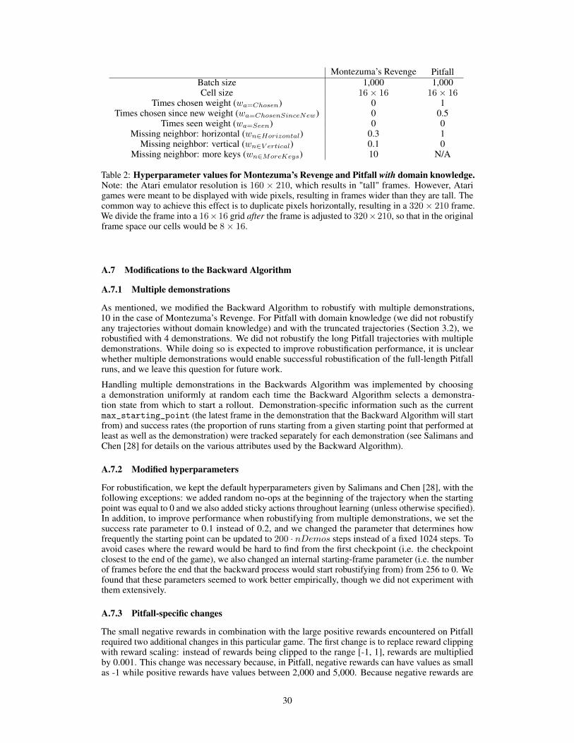
Montezuma’s Revenge PitfallBatch size 1,000 1,000Cell size 16× 16 16× 16

Times chosen weight (wa=Chosen) 0 1Times chosen since new weight (wa=ChosenSinceNew) 0 0.5

Times seen weight (wa=Seen) 0 0Missing neighbor: horizontal (wn∈Horizontal) 0.3 1

Missing neighbor: vertical (wn∈V ertical) 0.1 0Missing neighbor: more keys (wn∈MoreKeys) 10 N/A

Table 2: Hyperparameter values for Montezuma’s Revenge and Pitfall with domain knowledge.Note: the Atari emulator resolution is 160 × 210, which results in "tall" frames. However, Atarigames were meant to be displayed with wide pixels, resulting in frames wider than they are tall. Thecommon way to achieve this effect is to duplicate pixels horizontally, resulting in a 320× 210 frame.We divide the frame into a 16×16 grid after the frame is adjusted to 320×210, so that in the originalframe space our cells would be 8× 16.

A.7 Modifications to the Backward Algorithm

A.7.1 Multiple demonstrations

As mentioned, we modified the Backward Algorithm to robustify with multiple demonstrations,10 in the case of Montezuma’s Revenge. For Pitfall with domain knowledge (we did not robustifyany trajectories without domain knowledge) and with the truncated trajectories (Section 3.2), werobustified with 4 demonstrations. We did not robustify the long Pitfall trajectories with multipledemonstrations. While doing so is expected to improve robustification performance, it is unclearwhether multiple demonstrations would enable successful robustification of the full-length Pitfallruns, and we leave this question for future work.

Handling multiple demonstrations in the Backwards Algorithm was implemented by choosinga demonstration uniformly at random each time the Backward Algorithm selects a demonstra-tion state from which to start a rollout. Demonstration-specific information such as the currentmax_starting_point (the latest frame in the demonstration that the Backward Algorithm will startfrom) and success rates (the proportion of runs starting from a given starting point that performed atleast as well as the demonstration) were tracked separately for each demonstration (see Salimans andChen [28] for details on the various attributes used by the Backward Algorithm).

A.7.2 Modified hyperparameters

For robustification, we kept the default hyperparameters given by Salimans and Chen [28], with thefollowing exceptions: we added random no-ops at the beginning of the trajectory when the startingpoint was equal to 0 and we also added sticky actions throughout learning (unless otherwise specified).In addition, to improve performance when robustifying from multiple demonstrations, we set thesuccess rate parameter to 0.1 instead of 0.2, and we changed the parameter that determines howfrequently the starting point can be updated to 200 · nDemos steps instead of a fixed 1024 steps. Toavoid cases where the reward would be hard to find from the first checkpoint (i.e. the checkpointclosest to the end of the game), we also changed an internal starting-frame parameter (i.e. the numberof frames before the end that the backward process would start robustifying from) from 256 to 0. Wefound that these parameters seemed to work better empirically, though we did not experiment withthem extensively.

A.7.3 Pitfall-specific changes

The small negative rewards in combination with the large positive rewards encountered on Pitfallrequired two additional changes in this particular game. The first change is to replace reward clippingwith reward scaling: instead of rewards being clipped to the range [-1, 1], rewards are multipliedby 0.001. This change was necessary because, in Pitfall, negative rewards can have values as smallas -1 while positive rewards have values between 2,000 and 5,000. Because negative rewards are

30

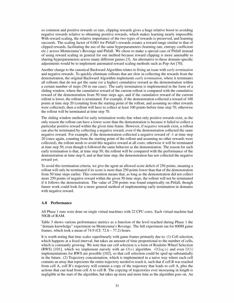
so common and positive rewards so rare, clipping rewards gives a huge relative boost to avoidingnegative rewards relative to obtaining positive rewards, which makes learning nearly impossible.With reward scaling, the relative importance of the two types of rewards is preserved, and learningsucceeds. The scaling factor of 0.001 for Pitfall’s rewards creates a reward range similar to that ofclipped rewards, facilitating the use of the same hyperparameters (learning rate, entropy coefficientetc.) across Montezuma’s Revenge and Pitfall. We chose to make a special case of Pitfall insteadof using reward scaling in general for our method because reward clipping is more amenable tosharing hyperparameters across many different games [3]. An alternative to these domain-specificadjustments would be to implement automated reward scaling methods such as Pop-Art [70].

Another change to the canonical Backward Algorithm relates to fixing an issue with early terminationand negative rewards. To quickly eliminate rollouts that are slow in collecting the rewards from thedemonstration, the original Backward Algorithm implements early termination, where it terminatesall rollouts that do not get the same (or a higher) cumulative reward as the demonstration withina certain number of steps (50 in our case). The early termination is implemented in the form of asliding window, where the cumulative reward of the current rollout is compared with the cumulativereward of the demonstration from 50 time steps ago, and if the cumulative reward of the currentrollout is lower, the rollout is terminated. For example, if the demonstration collected a reward of 100points at time step 20 (counting from the starting point of the rollout, and assuming no other rewardswere collected), then a rollout will have to collect at least 100 points before time step 70, otherwisethe rollout will be terminated at time step 70.

The sliding window method for early termination works fine when only positive rewards exist, as theonly reason the rollout can have a lower score than the demonstration is because it failed to collect aparticular positive reward within the given time frame. However, if negative rewards exist, a rolloutcan also be terminated by collecting a negative reward, even if the demonstration collected the samenegative reward. For example, if the demonstration collected a negative reward of -1 at time step20 (once again, counting from the starting point of the rollout and assuming no other rewards werecollected), the rollout needs to avoid this negative reward at all costs; otherwise it will be terminatedat time step 50, even though it followed the same behavior as the demonstration. The reason for suchearly termination is that, at time step 50, the rollout will be compared with the performance of thedemonstration at time step 0, and at that time step, the demonstration has not collected the negativereward yet.

To avoid this termination criteria, we give the agent an allowed score deficit of 250 points, meaning arollout will only be terminated if its score is more than 250 points lower than that of the demonstrationfrom 50 time steps earlier. This convention means that, as long as the demonstration did not collectmore 250 points of negative reward within the given 50 time steps, the rollout will not be terminatedif it follows the demonstration. The value of 250 points was found empirically on Pitfall, thoughfuture work could look for a more general method of implementing early termination in domainswith negative reward.

A.8 Performance

All Phase 1 runs were done on single virtual machines with 22 CPU cores. Each virtual machine had50GB of RAM.

Table 3 shows various performance metrics as a function of the level reached during Phase 1 the“domain knowledge” experiment on Montezuma’s Revenge. The full experiment ran for 600M gameframes, which took a mean of 74.9 (CI: 72.6 – 77.2) hours.

It is worth noting that time scales superlinearly with game frames primarily due to: (1) Cell selection,which happens at a fixed interval, but takes an amount of time proportional to the number of cells,which is constantly growing. We note that our cell selection is a form of Roulette-Wheel Selection(RWS) [101], which we implement naively with an O(n) algorithm. O(log n) and even O(1)implementations for RWS are possible [102], so that cell selection could be sped up substantiallyin the future. (2) Trajectory concatenation, which is implemented in a naive way where each cellcontains an array that represents the entire trajectory needed to reach it, such that if cell B was reachedfrom cell A, cell B’s trajectory will contain a copy of the trajectory that leads to cell A, plus theactions that can lead from cell A to cell B. The copying of trajectories ever increasing in length isnegligible at the start of the algorithm, but takes up more and more time as the algorithm goes on. An

31

Level Solved % Game Frames(excl. replay) Time (hours)

HypotheticalGame Frames(incl. replay)

1 100% 58M (53M – 62M) 0.9 (0.9 – 1.0) 1.5B (1.3B – 1.6B)2 100% 104M (97M – 111M) 2.5 (2.3 – 2.7) 4.3B (3.9B – 4.6B)3 100% 173M (164M – 182M) 6.8 (6.2 – 7.3) 12B (12B – 13B)4 100% 242M (230M – 253M) 12.7 (11.7 – 13.6) 24B (23B – 26B)5 100% 305M (292M – 318M) 19.9 (18.6 – 21.3) 38B (36B – 41B)6 100% 373M (358M – 388M) 29.4 (27.8 – 31.2) 57B (53B – 60B)7 100% 432M (416M – 448M) 39.1 (37.0 – 41.2) 75B (71B – 79B)8 94% 487M (471M – 503M) 49.8 (47.4 – 52.1) 96B (92B – 101B)9 70% 533M (518M – 548M) 61.4 (58.5 – 64.3) 117B (113B – 121B)10 38% 561M (550M – 572M) 70.4 (67.7 – 73.2) 139B (134B – 144B)11 12% 582M (570M – 595M) 77.6 (72.9 – 82.0) 151B (147B – 155B)

Table 3: Mean computational complexity to reach different levels for Montezuma’s Revengewith domain knowledge. The “Game frame (incl. replay)” metric shows the number of game framesthat would have been played if we replayed trajectories instead of resetting the emulator state. Itis a hypothetical metric, since we did not replay the trajectories, but instead reset the environment.The “Solved %” column shows the proportion of runs that solved a given level. All other metrics arecomputed only for the subset of runs that did solve the level.

alternative representation with better memory and computational efficiency would be to representtrajectories as linked lists of actions, and in reverse order, so that each action links to its predecessor.With this representation, if cell B is reached from cell A, only the actions leading from cell A to cellB need to be stored in cell B, with the first of these actions linking to the last action needed to reachcell A, which means that adding cell B would take constant time, instead of a time proportional tothe length of the longest trajectories in memory. Further, the amount of memory would also growlinearly, and the number of actions stored in memory would be bounded by the number of actionsever taken during exploration.

For Montezuma’s Revenge without domain knowledge, performance metrics are shown in Table 4.The full experiment ran for 1.2B game frames, which took 26.9 (CI: 25.6 – 28.2) hours. It is notablethat this is faster than the experiment with domain knowledge in spite of processing twice as manyframes. This is likely due to the same reasons that domain knowledge runs get slower over time: runswithout domain knowledge find fewer cells and shorter trajectories, and are thus less affected by theslowdown.

Level Solved % Game Frames(excl. replay) Time (hours)

HypotheticalGame Frames(incl. replay)

1 57% 640M (567M – 711M) 10.8 (9.5 – 12.0) 33B (28B – 37B)2 1% 592M (592M – 592M) 11.4 (11.4 – 11.4) 32B (32B – 32B)

Table 4: Mean computational complexity to reach different levels for Montezuma’s Revengewithout domain knowledge. The “Game frame (incl. replay)” metric shows the number of gameframes that would have been played if we replayed trajectories instead of resetting the emulator state.It is a hypothetical metric, since we did not replay the trajectories, but instead reset the environment.The “Solved %” column shows the proportion of runs that solved a given level. All other metrics arecomputed only for the subset of runs that did solve the level.

For Pitfall with domain knowledge, the threshold at which to compare game frames is not as clear asit is for Montezuma’s Revenge. In order to include data from all of our 40 runs, we report the requiredgame frames for reaching the lowest score achieved out of those runs, which is 47, 534. Reachingthis threshold required a mean of 794.0M (CI: 715.9M – 869.8M) game frames, which takes 25.0(CI: 21.4 – 28.3) hours, and it would have required a mean of 100.8B (CI: 84.1B – 116.0B) game

32

frames if trajectories had to be replayed from the start of the game. The full experiment lasted for4.0B game frames, which took a mean of 186.3 (CI: 184.9 – 187.8) hours. The full experiment wouldhave required 1,060.4B (CI: 1,048.5B – 1,071.7B) game frames if trajectories had to be replayedfrom the start of the game.

Because Pitfall without domain knowledge did not obtain any rewards, it is hard to define goodthresholds at which to compare game frames. In addition, regardless of the threshold we choose, theresulting data would not be representative of the resources Go-Explore would need to make progresson Pitfall (instead, it would represent the resource usage when Go-Explore fails to make progress).For those two reasons, we do not include Pitfall without domain knowledge in the remainder of thissection.

We did not monitor the precise memory usage of Phase 1, beyond the fact that all our runs succeededon machines with 50GB of RAM. Another indicator is the size of the serialized checkpoints producedat the end of each run, as these checkpoints contain all the necessary data to run Go-Explore,including the complete set of all cells, the metadata used in cell selection (see Appendix A.5), andthe trajectories needed to reach the cells. Uncompressed, these files serialized using pickle havea mean size of 341.2MB (CI: 292.3MB – 389.3MB) in the case of Montezuma’s Revenge withoutdomain knowledge, and 2.8GB (CI: 2.7GB – 2.9GB) with domain knowledge. For Pitfall with domainknowledge, the mean uncompressed checkpoint size was 1.30GB (CI: 1.29GB – 1.31GB).

For robustification, each run used 16 workers, each equipped with a single GPU, for a total of 16GPUs per run. For Montezuma’s Revenge without domain knowledge, runs lasted up to 5B gameframes though the selected checkpoints were produced after a mean of 4.35B (CI: 4.27B – 4.45B)game frames (which took a mean of 2.4 (CI: 2.4 – 2.5) days). For Montezuma’s Revenge with domainknowledge, runs lasted up to 10B game frames but selected checkpoints were produced after a meanof 4.59B (CI: 3.09B – 5.91B) game frames, which took a mean of 2.6 (CI: 1.8 – 3.3) days. ForPitfall with domain knowledge, runs lasted for about 12B game frames and selected checkpoints wereproduced after a mean of 8.20B (CI: 6.73B – 9.74B) game frames, which took a mean of 4.5 (CI: 3.7– 5.3) days.

A.9 Scores

Table 5 compares the results of Go-Explore with many other algorithms. The scores for the otheralgorithms are with stochastic testing in the form of random no-ops, sticky actions, human restarts,or a combination thereof. In the case of Go-Explore, both random no-ops and sticky actions werepresent in testing. As mentioned in Section 2.1.3, Go-Explore was trained partially without stickyactions or random no-ops, whereas many of the algorithms in this table also handled stochasticitythroughout training.

33

Algorithm Montezuma’s Revenge PitfallSARSA [3, 103] 259 -Linear [3, 103] 10.7 -DQN [3, 68] 0 -286.1Gorila [74] 84 -

MP-EB [104] 0 -DDQN [67, 68] 42 -30Duel. DQN [68] 22 0Prior. DQN [69] 13 -15

A3C [105] 67 -78Pop-Art [70] 0 -3

DQN-CTS [4] 3,705 0A3C-CTS [4] 1,127 -259

BASS-hash [33] 238 -DQN-PixelCNN [36] 2,514 0

ES [71] 0 -Reactor [34] 2,643.5 -3.5

Feature-EB [35] 2,745 -C51 [72] 0 0UBE [38] 3,000 0

Rainbow [73] 154 0IMPALA [42] 2,643.5 -1.2

Ape-X [41] 2,500 -1DeepCS [37] 3,500 -186

RND [16] 11,347 -3PPO+CoEX [39] 11,540 -

Go-Explore 43,763 -Go-Explore

(domain knowledge) 666,474 59,494Go-Explore (best) 18,003,200 107,363

DQfD [26] 4,638 57TDC+CMC [45] 41,098 76,813

Ape-X DQfD [27] 29,384 3,997LfSD (best) [28] 74,500 -

Average Human [27] 4,753 6,464Human Expert [27] 34,900 47,821

Human World Record [78] 1,219,200 114,000

Table 5: Comparison to baselines for Montezuma’s Revenge and Pitfall. The second sectiongives the performance of imitation learning algorithms, while the third gives human performance.Results are given in order of first public release (including preprints). Many historical papers didnot consider Pitfall, in which case the score is displayed as “-”. Two references are given in caseswhere the score from a given method does not appear in its original paper, but appears in anotherpaper (usually in a comparison section).

34

A.10 Fine-grained cell representation for Pitfall without domain knowledge

As mentioned in Section 3.2, we attempted an experiment on Pitfall without domain knowledge usingthe same parameters as with Montezuma’s Revenge. This approach did not succeed, as Go-Explorequickly stopped finding new rooms and failed to find any rewards (Fig. 9). One potential reason forthis failure is that the downscaled cell representation optimized for Montezuma’s Revenge conflatestoo many states into the same cell in Pitfall. This hypothesis is supported by the fact that Go-Explorestops discovering new cells, both when measured post-hoc as domain knowledge cells (Fig. 9) and inthe downscaled representation of cells in which it is actually searching (Fig. 11).

0.0 0.5 1.0 1.5 2.0Game Frames 1e9

0

1000

2000

3000

4000

5000

W/O

Dom

ain

Know

ledg

e Ce

lls F

ound

Figure 11: Number of without-domain-knowledge cells found during Phase 1 on Pitfall withoutdomain knowledge. Most cells are found within the first 500M game frames, after which very fewnew cells are found. This observation suggests that Pitfall without domain knowledge fails becausethere are too many different states that are mapped to the same Go-Explore cell.

To resolve this issue, we looked at different cell representations that would be able to distinguish alarger number of states. A particularly promising cell representation assigns 16, rather than 8, differentpixel values to each pixel in the 11 × 8 downscaled representation. While this cell representationdoes result in a larger number of rooms visited and the number of downscaled cells found did notstagnate, the runs terminated prematurely due to exhausting the 50GB of memory available on thevirtual machine (Fig. 12). Better hardware, distributed computation, or algorithmic improvements areall potential methods to resolve this issue, but we leave their implementation to future work.

0 2 4 6Game Frames 1e8

5

10

15

20

25

30

35

Foun

d Ro

oms

(a) Number of rooms found

0 2 4 6Game Frames 1e8

0

100,000

200,000

300,000

400,000

500,000

600,000

W/O

Dom

ain

Know

ledg

e Ce

lls fo

und

(b) Number of cells found

0 2 4 6Game Frames 1e8

0

0

0

0

0

Best

Sco

re

(c) Maximum score in archive

Figure 12: Go-Explore Phase 1 on Pitfall without domain knowledge with a more fine-grained(16 different pixel values instead of 8) cell representation. While the number of rooms (a) andthe number of cells (b) found continues to increase, even after 600M game frames, the runs do notcontinue beyond this point because they run out of memory. Despite visiting more rooms, Go-Explorestill does not find any rewards, although it may have were it able to continue for longer (c). The noiseat the end of sub-figure (a) is caused by different runs crashing at different times. The plot showsthe mean and 95% bootstrapped confidence interval over 20 runs initially, but the number of runsdeclines over time. The first run crashes around 500M game frames.

35

A.11 Failure robustifying long trajectories in Pitfall

While Go-Explore on Pitfall with domain knowledge is able to find trajectories that score over 70,000points (Fig. 9), the Backward Algorithm was unable to robustify these trajectories (Fig. 13).

0.00 0.25 0.50 0.75 1.00 1.25 1.50 1.75 2.00Game Frames 1e10

0

10,000

20,000

30,000

40,000

50,000

60,000

70,000

Max

Sta

rting

Poi

nt

Demo 1Demo 2Demo 3Demo 4Demo 5

Figure 13: Maximum starting point over training when robustifying the full-length trajectoriesproduced by Go-Explore in Phase 1 on Pitfall with domain knowledge. Unlike in Fig. 5b, thelines in this figure represent separate robustification attempts, each of which was applied to a singledemonstration taken from different runs of Go-Explore Phase 1. None of the 5 robustification attemptsreaches a starting point near 0, meaning that robustification failed on these demonstrations. We didnot try to robustify from multiple demonstrations for want of time, although doing so may haveworked better.

A.12 Nearly identical states in Pitfall

Pitfall contains many rooms located in different parts of the game that contain the exact same objectsand hazards. These identical rooms can result in nearly identical-looking states that require differentactions to be navigated optimally (Fig. 14), and they indicate that Pitfall is a Partially ObservableMarkov Decision Process (POMDP). These nearly identical looking states can pose a problem, bothwhen robustifying trajectories that visit some of these states, and when designing a domain-agnosticcell representation that should, ideally, treat these states as being in different cells.

The general method for handling POMDPs is to condition the current action on all previouslyobserved states, for example by training a recurrent, rather than feed-forward, neural network. Forthe robustification phase our method already implements a recurrent layer in the neural network,but, possibly due to the way the network is trained with the Backward Algorithm (i.e. wheneverthe agent is started from a particular state, it is not presented with all states that would have comebefore), this recurrent layer does not appear to completely solve the issue (see also section 3.2).A similar approach could be applied for obtaining cell representations (e.g. a cell representationcould be conditioned on all observations of the trajectory to a particular state, rather than just theobservation at a particular state), but care would have to be taken to ensure that actually identical (ornearly identical) states are recognized as such.

36

direction in demonstration

direction in demonstration

Figure 14: Two nearly identical looking states that require different actions to be navigatedoptimally. The two screenshots are taken from the same Go-Explore demonstration, but at differenttimes. The rooms are conceptually identical: they both contain a blue pool, a swinging vine, threerolling logs, and a scorpion. However, because the two rooms are located in different areas of thegame, the correct actions for navigating the two rooms can be different. In this case, the Go-Exploredemonstration navigates the left room right to left, whereas it navigates the right room from left toright. When training a policy in this situation, there will be many similar looking states that requireopposite actions. While the moving aspects of the room (i.e. the vine, the logs, and the scorpion)are likely to be in different locations in the two rooms of the demonstration, the fact that they willalso be in different locations when entering the rooms at different times makes them poor featuresfor differentiation. Probably the most informative features that can be used to determine in whichdirection to move are the score counter and the clock (the white numbers in the top left of eachimage), though, in practice, these small, frequently-changing features seem insufficient to provide thenecessary guidance.

37