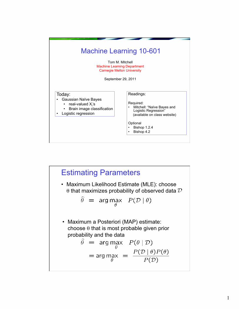
1

Machine Learning 10-601 Tom M. Mitchell

Machine Learning Department Carnegie Mellon University

September 29, 2011

Today: •  Gaussian Naïve Bayes

•  real-valued Xi’s •  Brain image classification

•  Logistic regression

Readings: Required: •  Mitchell: “Naïve Bayes and

Logistic Regression” (available on class website) Optional •  Bishop 1.2.4 •  Bishop 4.2

Estimating Parameters •  Maximum Likelihood Estimate (MLE): choose θ that maximizes probability of observed data

•  Maximum a Posteriori (MAP) estimate: choose θ that is most probable given prior probability and the data

2

Recently: •  Bayes classifiers to learn P(Y|X) •  MLE and MAP estimates for parameters of P •  Conditional independence •  Naïve Bayes à make Bayesian learning practical •  Text classification

Today: •  Naïve Bayes and continuous variables Xi:

•  Gaussian Naïve Bayes classifier •  Learn P(Y|X) directly

•  Logistic regression, Regularization, Gradient ascent •  Naïve Bayes or Logistic Regression?

•  Generative vs. Discriminative classifiers

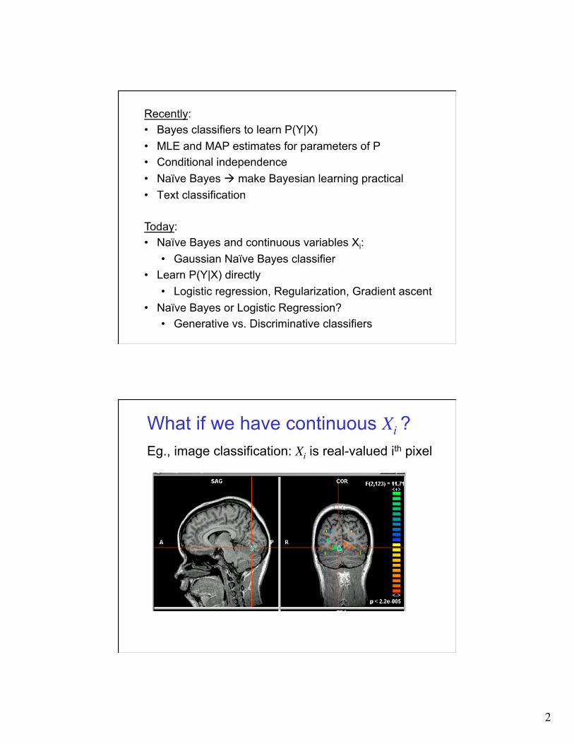
What if we have continuous Xi ? Eg., image classification: Xi is real-valued ith pixel

3

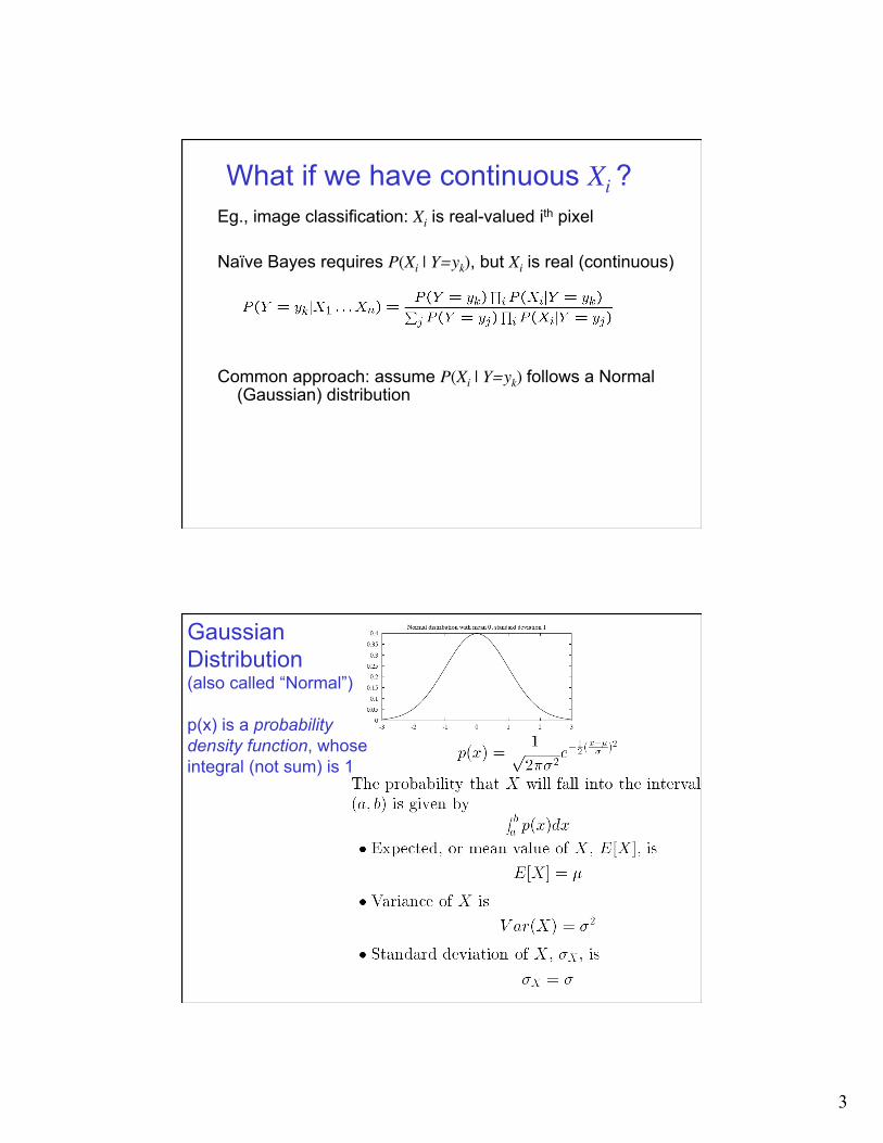
What if we have continuous Xi ? Eg., image classification: Xi is real-valued ith pixel Naïve Bayes requires P(Xi | Y=yk), but Xi is real (continuous) Common approach: assume P(Xi | Y=yk) follows a Normal

(Gaussian) distribution

Gaussian Distribution (also called “Normal”) p(x) is a probability density function, whose integral (not sum) is 1

4

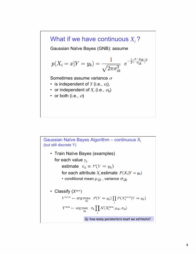
What if we have continuous Xi ? Gaussian Naïve Bayes (GNB): assume Sometimes assume variance σ •  is independent of Y (i.e., σi), •  or independent of Xi (i.e., σk) •  or both (i.e., σ)

•  Train Naïve Bayes (examples) for each value yk estimate for each attribute Xi estimate

•  conditional mean , variance •  Classify (Xnew)

Gaussian Naïve Bayes Algorithm – continuous Xi (but still discrete Y)

Q: how many parameters must we estimate?

5

Estimating Parameters: Y discrete, Xi continuous

Maximum likelihood estimates:

jth training example

δ()=1 if (Yj=yk) else 0

ith feature kth class

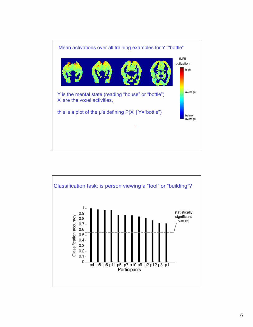
GNB Example: Classify a person’s cognitive state, based on brain image

•  reading a sentence or viewing a picture? •  reading the word describing a “Tool” or “Building”? •  answering the question, or getting confused?

6

Y is the mental state (reading “house” or “bottle”) Xi are the voxel activities, this is a plot of the µ’s defining P(Xi | Y=“bottle”)

fMRI activation

high

below average

average

Mean activations over all training examples for Y=“bottle”

Classification task: is person viewing a “tool” or “building”?

p4 p8 p6 p11 p5 p7 p10 p9 p2 p12 p3 p10

0.10.20.30.40.50.60.70.80.9

1

Participants

Cla

ssifi

catio

n ac

cura

cy statistically significant

p<0.05

Cla

ssifi

catio

n ac

cura

cy

7

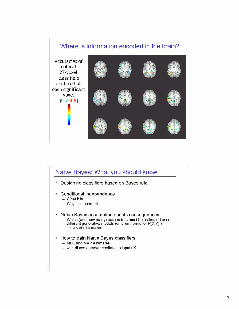
Where is information encoded in the brain?

Accuracies of cubical 27-voxel classifiers

centered at each significant

voxel [0.7-0.8]

Naïve Bayes: What you should know •  Designing classifiers based on Bayes rule

•  Conditional independence –  What it is –  Why it’s important

•  Naïve Bayes assumption and its consequences –  Which (and how many) parameters must be estimated under

different generative models (different forms for P(X|Y) ) •  and why this matters

•  How to train Naïve Bayes classifiers –  MLE and MAP estimates –  with discrete and/or continuous inputs Xi

8

Questions to think about: •  Can you use Naïve Bayes for a combination of

discrete and real-valued Xi?

•  How can we easily model just 2 of n attributes as dependent?

•  What does the decision surface of a Naïve Bayes classifier look like?

•  How would you select a subset of Xi’s?

Logistic Regression

Machine Learning 10-601

Tom M. Mitchell Machine Learning Department

Carnegie Mellon University

September 29, 2011

Required reading: •  Mitchell draft chapter (see course website)

Recommended reading: •  Ng and Jordan paper (see course website)

9

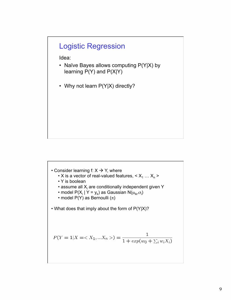
Logistic Regression Idea: •  Naïve Bayes allows computing P(Y|X) by

learning P(Y) and P(X|Y)

•  Why not learn P(Y|X) directly?

•  Consider learning f: X à Y, where •  X is a vector of real-valued features, < X1 … Xn > •  Y is boolean •  assume all Xi are conditionally independent given Y •  model P(Xi | Y = yk) as Gaussian N(µik,σi) •  model P(Y) as Bernoulli (π)

•  What does that imply about the form of P(Y|X)?

10

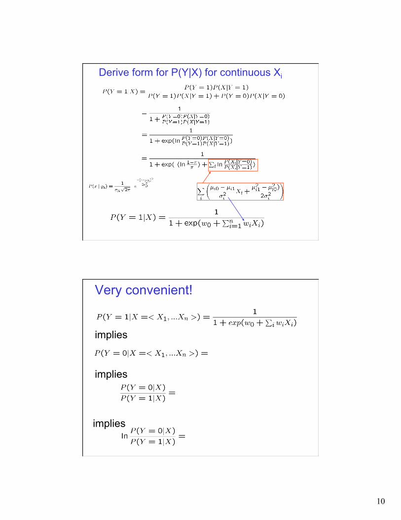
Derive form for P(Y|X) for continuous Xi

Very convenient!

implies

implies

implies

11

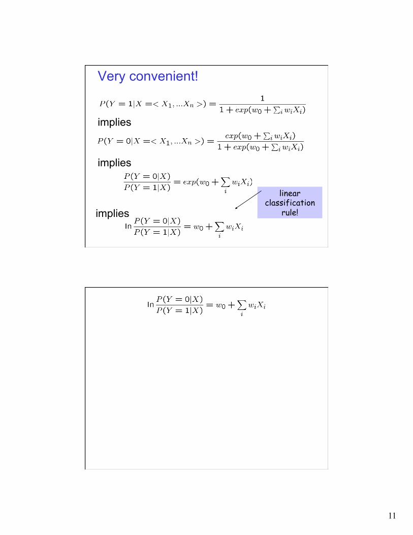
Very convenient!

implies

implies

implies

linear classification

rule!

12

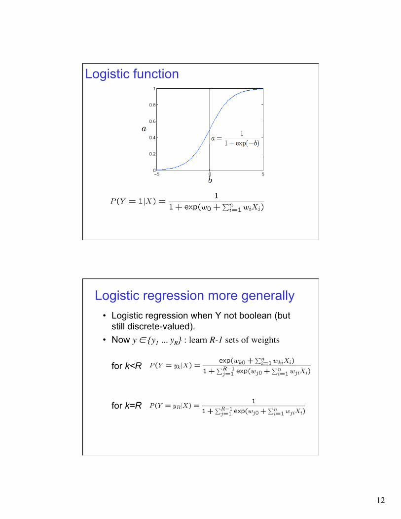
Logistic function

Logistic regression more generally •  Logistic regression when Y not boolean (but

still discrete-valued). •  Now y ∈ {y1 ... yR} : learn R-1 sets of weights

for k<R

for k=R

13

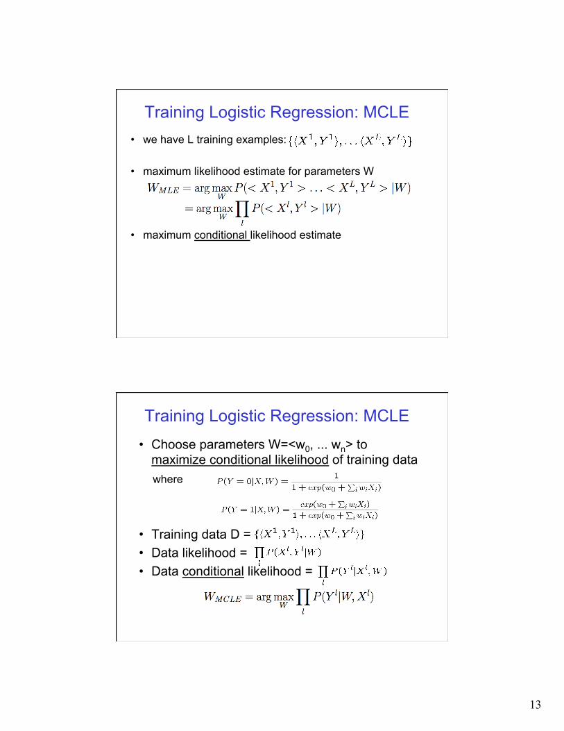
Training Logistic Regression: MCLE •  we have L training examples:

•  maximum likelihood estimate for parameters W

•  maximum conditional likelihood estimate

Training Logistic Regression: MCLE •  Choose parameters W=<w0, ... wn> to

maximize conditional likelihood of training data

•  Training data D = •  Data likelihood = •  Data conditional likelihood =

where

14

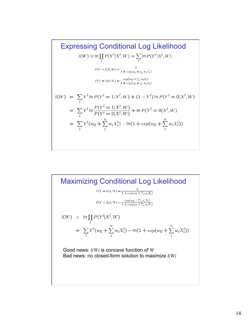
Expressing Conditional Log Likelihood

Maximizing Conditional Log Likelihood

Good news: l(W) is concave function of W Bad news: no closed-form solution to maximize l(W)

15

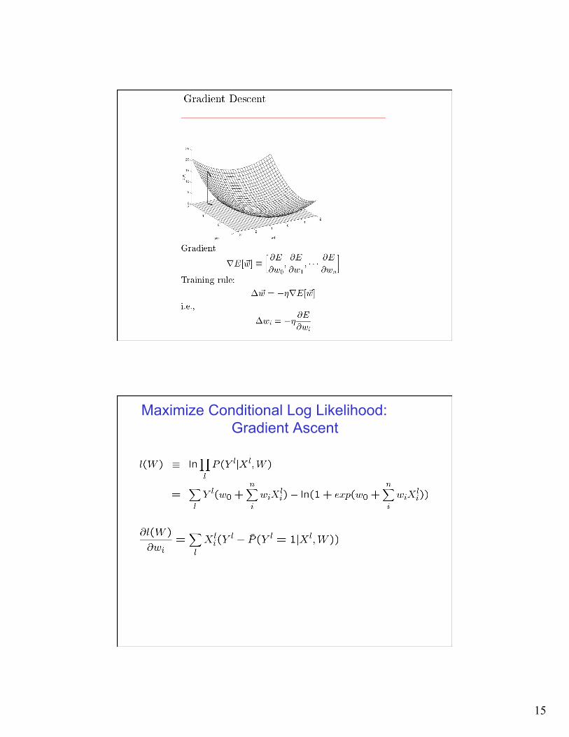
Maximize Conditional Log Likelihood: Gradient Ascent

16

Maximize Conditional Log Likelihood: Gradient Ascent

Gradient ascent algorithm: iterate until change < ε For all i, repeat

That’s all for M(C)LE. How about MAP?

•  One common approach is to define priors on W –  Normal distribution, zero mean, identity covariance

•  Helps avoid very large weights and overfitting •  MAP estimate

•  let’s assume Gaussian prior: W ~ N(0, σ)

17

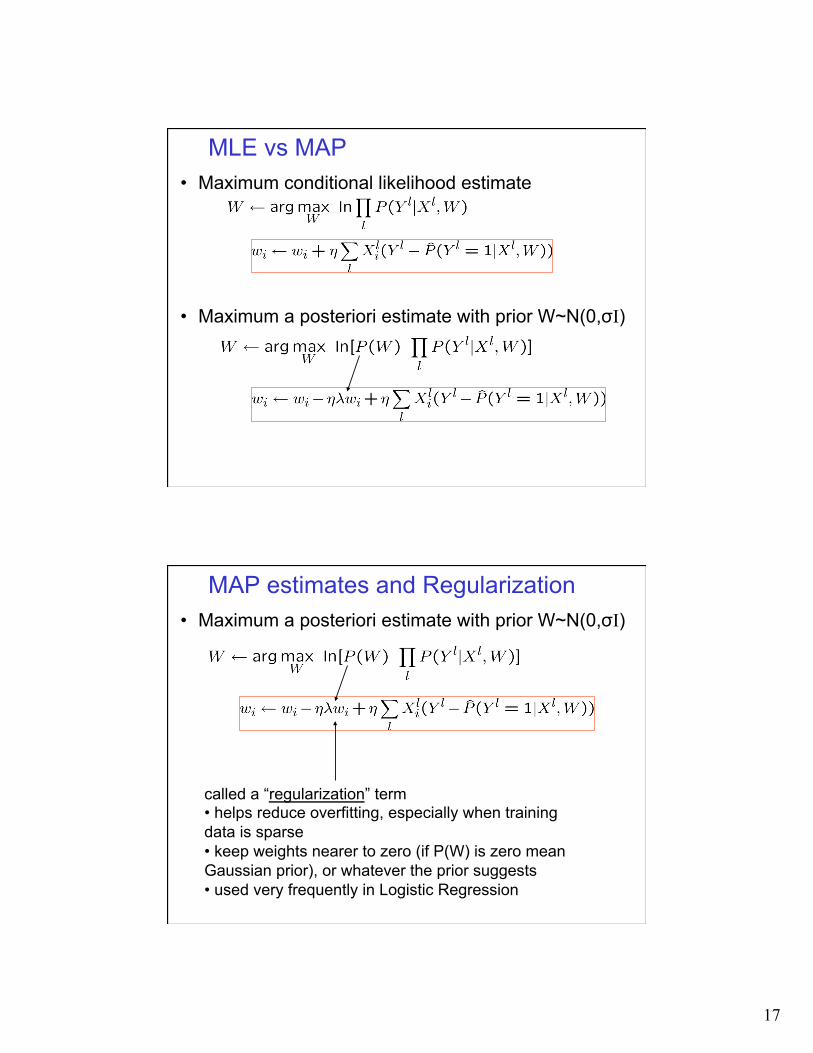
MLE vs MAP •  Maximum conditional likelihood estimate

•  Maximum a posteriori estimate with prior W~N(0,σI)

MAP estimates and Regularization •  Maximum a posteriori estimate with prior W~N(0,σI)

called a “regularization” term •  helps reduce overfitting, especially when training data is sparse •  keep weights nearer to zero (if P(W) is zero mean Gaussian prior), or whatever the prior suggests •  used very frequently in Logistic Regression

18

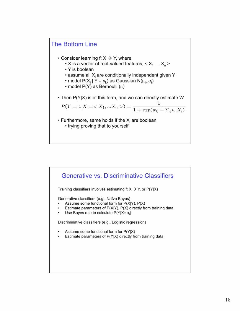
•  Consider learning f: X à Y, where •  X is a vector of real-valued features, < X1 … Xn > •  Y is boolean •  assume all Xi are conditionally independent given Y •  model P(Xi | Y = yk) as Gaussian N(µik,σi) •  model P(Y) as Bernoulli (π)

•  Then P(Y|X) is of this form, and we can directly estimate W

•  Furthermore, same holds if the Xi are boolean •  trying proving that to yourself

The Bottom Line

Generative vs. Discriminative Classifiers

Training classifiers involves estimating f: X à Y, or P(Y|X) Generative classifiers (e.g., Naïve Bayes) •  Assume some functional form for P(X|Y), P(X) •  Estimate parameters of P(X|Y), P(X) directly from training data •  Use Bayes rule to calculate P(Y|X= xi)

Discriminative classifiers (e.g., Logistic regression) •  Assume some functional form for P(Y|X) •  Estimate parameters of P(Y|X) directly from training data

19

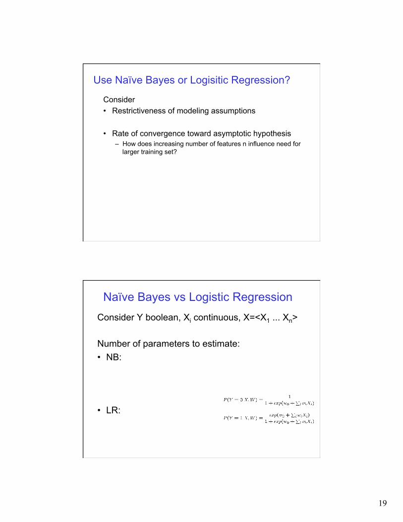
Use Naïve Bayes or Logisitic Regression?

Consider •  Restrictiveness of modeling assumptions •  Rate of convergence toward asymptotic hypothesis

–  How does increasing number of features n influence need for larger training set?

Naïve Bayes vs Logistic Regression Consider Y boolean, Xi continuous, X=<X1 ... Xn> Number of parameters to estimate: •  NB:

•  LR:

20

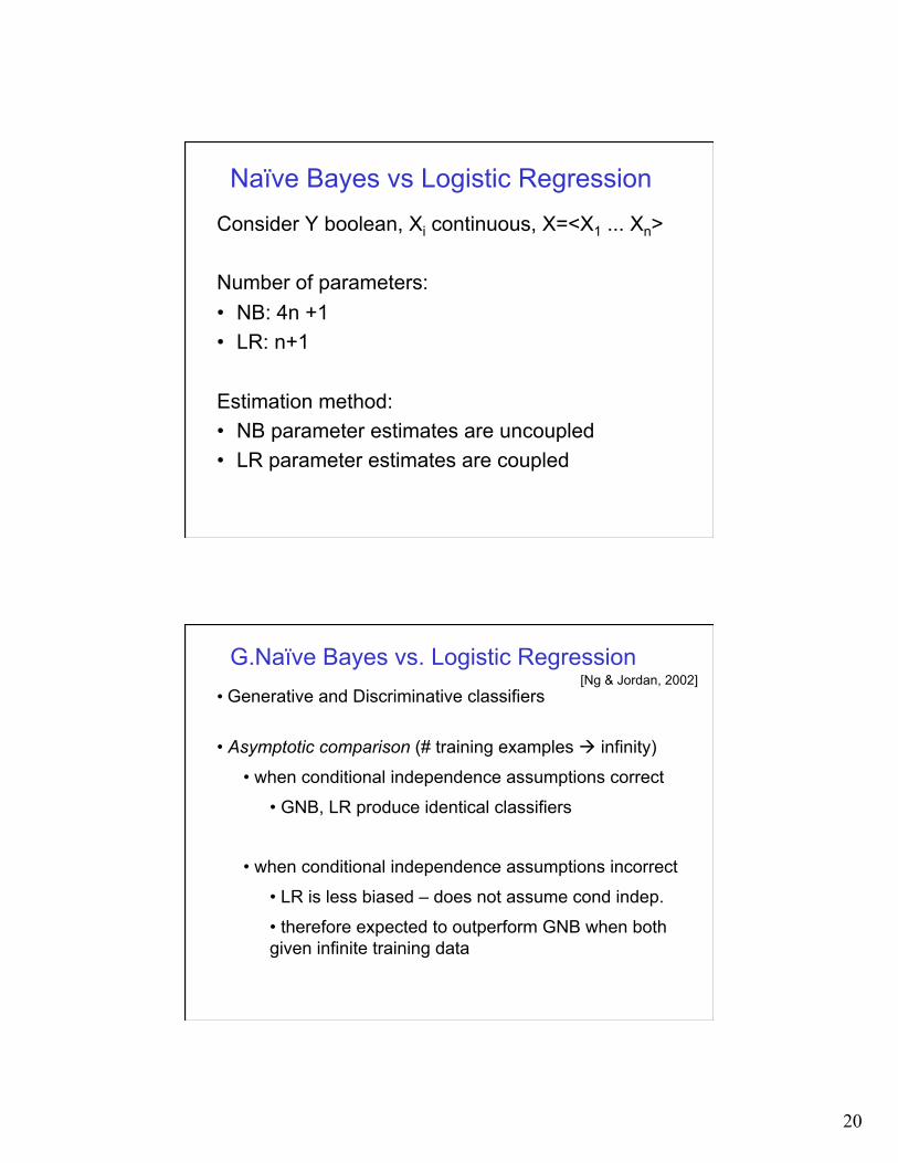
Naïve Bayes vs Logistic Regression Consider Y boolean, Xi continuous, X=<X1 ... Xn> Number of parameters: •  NB: 4n +1 •  LR: n+1

Estimation method: •  NB parameter estimates are uncoupled •  LR parameter estimates are coupled

G.Naïve Bayes vs. Logistic Regression •  Generative and Discriminative classifiers

•  Asymptotic comparison (# training examples à infinity)

•  when conditional independence assumptions correct

•  GNB, LR produce identical classifiers

•  when conditional independence assumptions incorrect

•  LR is less biased – does not assume cond indep.

•  therefore expected to outperform GNB when both given infinite training data

[Ng & Jordan, 2002]

21

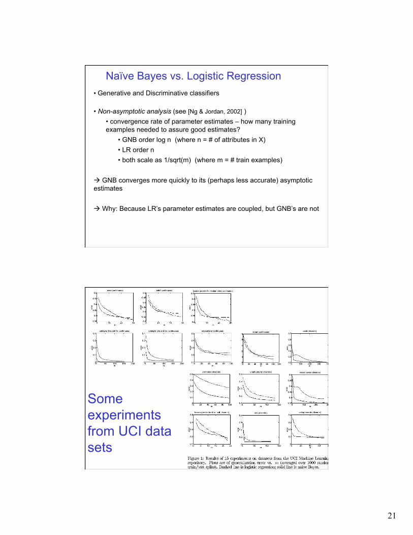
Naïve Bayes vs. Logistic Regression •  Generative and Discriminative classifiers

•  Non-asymptotic analysis (see [Ng & Jordan, 2002] ) •  convergence rate of parameter estimates – how many training examples needed to assure good estimates?

•  GNB order log n (where n = # of attributes in X) •  LR order n •  both scale as 1/sqrt(m) (where m = # train examples)

à GNB converges more quickly to its (perhaps less accurate) asymptotic estimates

à Why: Because LR’s parameter estimates are coupled, but GNB’s are not

Some experiments from UCI data sets

22

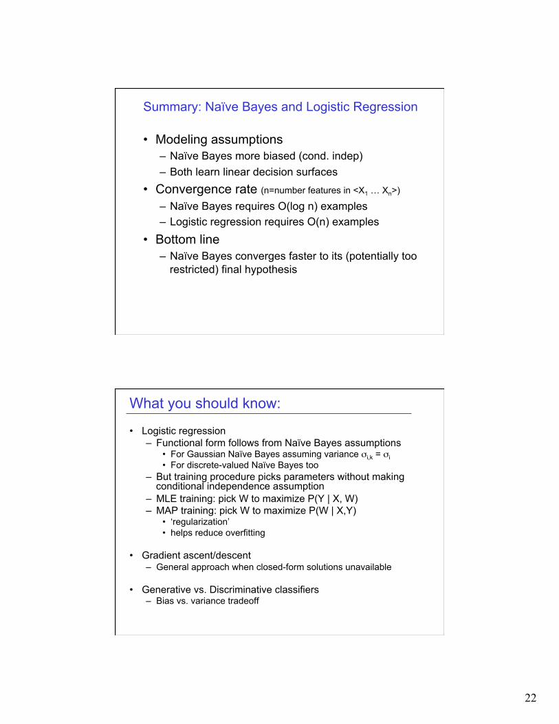
Summary: Naïve Bayes and Logistic Regression

•  Modeling assumptions –  Naïve Bayes more biased (cond. indep) –  Both learn linear decision surfaces

•  Convergence rate (n=number features in <X1 … Xn>) –  Naïve Bayes requires O(log n) examples –  Logistic regression requires O(n) examples

•  Bottom line –  Naïve Bayes converges faster to its (potentially too

restricted) final hypothesis

What you should know:

•  Logistic regression –  Functional form follows from Naïve Bayes assumptions

•  For Gaussian Naïve Bayes assuming variance σi,k = σi •  For discrete-valued Naïve Bayes too

–  But training procedure picks parameters without making conditional independence assumption

–  MLE training: pick W to maximize P(Y | X, W) –  MAP training: pick W to maximize P(W | X,Y)

•  ‘regularization’ •  helps reduce overfitting

•  Gradient ascent/descent –  General approach when closed-form solutions unavailable

•  Generative vs. Discriminative classifiers –  Bias vs. variance tradeoff