Backpropagation+

Deep Learning

1

10-601 Introduction to Machine Learning

Matt GormleyLecture 13

Mar 1, 2018

Machine Learning DepartmentSchool of Computer ScienceCarnegie Mellon University

Reminders

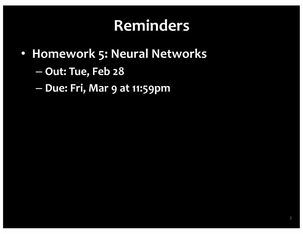
• Homework 5: Neural Networks– Out: Tue, Feb 28– Due: Fri, Mar 9 at 11:59pm

2

Q&A

3

BACKPROPAGATION

4

A Recipe for Machine Learning

1. Given training data: 3. Define goal:

5

Background

2. Choose each of these:– Decision function

– Loss function

4. Train with SGD:(take small steps opposite the gradient)

Approaches to Differentiation

• Question 1:When can we compute the gradients of the parameters of an arbitrary neural network?

• Question 2:When can we make the gradient computation efficient?

6

Training

Approaches to Differentiation

1. Finite Difference Method– Pro: Great for testing implementations of backpropagation– Con: Slow for high dimensional inputs / outputs– Required: Ability to call the function f(x) on any input x

2. Symbolic Differentiation– Note: The method you learned in high-school– Note: Used by Mathematica / Wolfram Alpha / Maple– Pro: Yields easily interpretable derivatives– Con: Leads to exponential computation time if not carefully implemented– Required: Mathematical expression that defines f(x)

3. Automatic Differentiation - Reverse Mode– Note: Called Backpropagation when applied to Neural Nets– Pro: Computes partial derivatives of one output f(x)i with respect to all inputs xj in time proportional

to computation of f(x)– Con: Slow for high dimensional outputs (e.g. vector-valued functions)– Required: Algorithm for computing f(x)

4. Automatic Differentiation - Forward Mode– Note: Easy to implement. Uses dual numbers.– Pro: Computes partial derivatives of all outputs f(x)i with respect to one input xj in time proportional

to computation of f(x)– Con: Slow for high dimensional inputs (e.g. vector-valued x)– Required: Algorithm for computing f(x)

7

Training

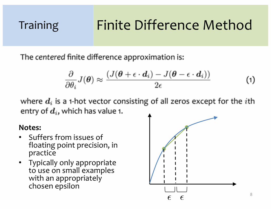
Finite Difference Method

Notes:• Suffers from issues of

floating point precision, in practice

• Typically only appropriate to use on small examples with an appropriately chosen epsilon

8

Training

Symbolic Differentiation

9

Training

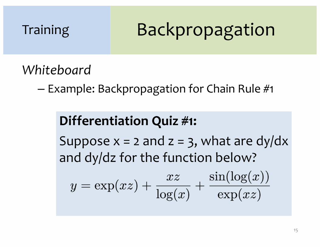
Differentiation Quiz #1:Suppose x = 2 and z = 3, what are dy/dx and dy/dz for the function below?

Symbolic Differentiation

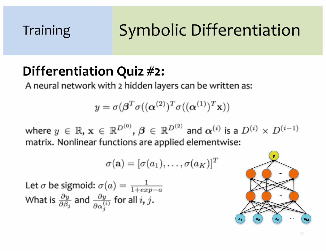
Differentiation Quiz #2:

11

Training

…

…

…

Chain Rule

Whiteboard– Chain Rule of Calculus

12

Training

Chain Rule

13

Training

2.2. NEURAL NETWORKS AND BACKPROPAGATION

x to J , but also a manner of carrying out that computation in terms of the intermediatequantities a, z, b, y. Which intermediate quantities to use is a design decision. In thisway, the arithmetic circuit diagram of Figure 2.1 is differentiated from the standard neuralnetwork diagram in two ways. A standard diagram for a neural network does not show thischoice of intermediate quantities nor the form of the computations.

The topologies presented in this section are very simple. However, we will later (Chap-ter 5) how an entire algorithm can define an arithmetic circuit.

2.2.2 BackpropagationThe backpropagation algorithm (Rumelhart et al., 1986) is a general method for computingthe gradient of a neural network. Here we generalize the concept of a neural network toinclude any arithmetic circuit. Applying the backpropagation algorithm on these circuitsamounts to repeated application of the chain rule. This general algorithm goes under manyother names: automatic differentiation (AD) in the reverse mode (Griewank and Corliss,1991), analytic differentiation, module-based AD, autodiff, etc. Below we define a forwardpass, which computes the output bottom-up, and a backward pass, which computes thederivatives of all intermediate quantities top-down.

Chain Rule At the core of the backpropagation algorithm is the chain rule. The chainrule allows us to differentiate a function f defined as the composition of two functions gand h such that f = (g �h). If the inputs and outputs of g and h are vector-valued variablesthen f is as well: h : RK

! RJ and g : RJ! RI

) f : RK! RI . Given an input

vector x = {x1

, x2

, . . . , xK}, we compute the output y = {y1

, y2

, . . . , yI}, in terms of anintermediate vector u = {u

1

, u2

, . . . , uJ}. That is, the computation y = f(x) = g(h(x))can be described in a feed-forward manner: y = g(u) and u = h(x). Then the chain rulemust sum over all the intermediate quantities.

dyi

dxk=

JX

j=1

dyi

duj

duj

dxk, 8i, k (2.3)

If the inputs and outputs of f , g, and h are all scalars, then we obtain the familiar formof the chain rule:

dy

dx=

dy

du

du

dx(2.4)

Binary Logistic Regression Binary logistic regression can be interpreted as a arithmeticcircuit. To compute the derivative of some loss function (below we use regression) withrespect to the model parameters ✓, we can repeatedly apply the chain rule (i.e. backprop-agation). Note that the output q below is the probability that the output label takes on thevalue 1. y⇤ is the true output label. The forward pass computes the following:

J = y⇤log q + (1 � y⇤

) log(1 � q) (2.5)

where q = P✓

(Yi = 1|x) =

1

1 + exp(�

PDj=0

✓jxj)(2.6)

13

2.2. NEURAL NETWORKS AND BACKPROPAGATION

x to J , but also a manner of carrying out that computation in terms of the intermediatequantities a, z, b, y. Which intermediate quantities to use is a design decision. In thisway, the arithmetic circuit diagram of Figure 2.1 is differentiated from the standard neuralnetwork diagram in two ways. A standard diagram for a neural network does not show thischoice of intermediate quantities nor the form of the computations.

The topologies presented in this section are very simple. However, we will later (Chap-ter 5) how an entire algorithm can define an arithmetic circuit.

2.2.2 BackpropagationThe backpropagation algorithm (Rumelhart et al., 1986) is a general method for computingthe gradient of a neural network. Here we generalize the concept of a neural network toinclude any arithmetic circuit. Applying the backpropagation algorithm on these circuitsamounts to repeated application of the chain rule. This general algorithm goes under manyother names: automatic differentiation (AD) in the reverse mode (Griewank and Corliss,1991), analytic differentiation, module-based AD, autodiff, etc. Below we define a forwardpass, which computes the output bottom-up, and a backward pass, which computes thederivatives of all intermediate quantities top-down.

Chain Rule At the core of the backpropagation algorithm is the chain rule. The chainrule allows us to differentiate a function f defined as the composition of two functions gand h such that f = (g �h). If the inputs and outputs of g and h are vector-valued variablesthen f is as well: h : RK

! RJ and g : RJ! RI

) f : RK! RI . Given an input

vector x = {x1

, x2

, . . . , xK}, we compute the output y = {y1

, y2

, . . . , yI}, in terms of anintermediate vector u = {u

1

, u2

, . . . , uJ}. That is, the computation y = f(x) = g(h(x))can be described in a feed-forward manner: y = g(u) and u = h(x). Then the chain rulemust sum over all the intermediate quantities.

dyi

dxk=

JX

j=1

dyi

duj

duj

dxk, 8i, k (2.3)

If the inputs and outputs of f , g, and h are all scalars, then we obtain the familiar formof the chain rule:

dy

dx=

dy

du

du

dx(2.4)

Binary Logistic Regression Binary logistic regression can be interpreted as a arithmeticcircuit. To compute the derivative of some loss function (below we use regression) withrespect to the model parameters ✓, we can repeatedly apply the chain rule (i.e. backprop-agation). Note that the output q below is the probability that the output label takes on thevalue 1. y⇤ is the true output label. The forward pass computes the following:

J = y⇤log q + (1 � y⇤

) log(1 � q) (2.5)

where q = P✓

(Yi = 1|x) =

1

1 + exp(�

PDj=0

✓jxj)(2.6)

13

Chain Rule:Given:

…

Chain Rule

14

Training

2.2. NEURAL NETWORKS AND BACKPROPAGATION

x to J , but also a manner of carrying out that computation in terms of the intermediatequantities a, z, b, y. Which intermediate quantities to use is a design decision. In thisway, the arithmetic circuit diagram of Figure 2.1 is differentiated from the standard neuralnetwork diagram in two ways. A standard diagram for a neural network does not show thischoice of intermediate quantities nor the form of the computations.

The topologies presented in this section are very simple. However, we will later (Chap-ter 5) how an entire algorithm can define an arithmetic circuit.

2.2.2 BackpropagationThe backpropagation algorithm (Rumelhart et al., 1986) is a general method for computingthe gradient of a neural network. Here we generalize the concept of a neural network toinclude any arithmetic circuit. Applying the backpropagation algorithm on these circuitsamounts to repeated application of the chain rule. This general algorithm goes under manyother names: automatic differentiation (AD) in the reverse mode (Griewank and Corliss,1991), analytic differentiation, module-based AD, autodiff, etc. Below we define a forwardpass, which computes the output bottom-up, and a backward pass, which computes thederivatives of all intermediate quantities top-down.

Chain Rule At the core of the backpropagation algorithm is the chain rule. The chainrule allows us to differentiate a function f defined as the composition of two functions gand h such that f = (g �h). If the inputs and outputs of g and h are vector-valued variablesthen f is as well: h : RK

! RJ and g : RJ! RI

) f : RK! RI . Given an input

vector x = {x1

, x2

, . . . , xK}, we compute the output y = {y1

, y2

, . . . , yI}, in terms of anintermediate vector u = {u

1

, u2

, . . . , uJ}. That is, the computation y = f(x) = g(h(x))can be described in a feed-forward manner: y = g(u) and u = h(x). Then the chain rulemust sum over all the intermediate quantities.

dyi

dxk=

JX

j=1

dyi

duj

duj

dxk, 8i, k (2.3)

If the inputs and outputs of f , g, and h are all scalars, then we obtain the familiar formof the chain rule:

dy

dx=

dy

du

du

dx(2.4)

Binary Logistic Regression Binary logistic regression can be interpreted as a arithmeticcircuit. To compute the derivative of some loss function (below we use regression) withrespect to the model parameters ✓, we can repeatedly apply the chain rule (i.e. backprop-agation). Note that the output q below is the probability that the output label takes on thevalue 1. y⇤ is the true output label. The forward pass computes the following:

J = y⇤log q + (1 � y⇤

) log(1 � q) (2.5)

where q = P✓

(Yi = 1|x) =

1

1 + exp(�

PDj=0

✓jxj)(2.6)

13

2.2. NEURAL NETWORKS AND BACKPROPAGATION

x to J , but also a manner of carrying out that computation in terms of the intermediatequantities a, z, b, y. Which intermediate quantities to use is a design decision. In thisway, the arithmetic circuit diagram of Figure 2.1 is differentiated from the standard neuralnetwork diagram in two ways. A standard diagram for a neural network does not show thischoice of intermediate quantities nor the form of the computations.

The topologies presented in this section are very simple. However, we will later (Chap-ter 5) how an entire algorithm can define an arithmetic circuit.

2.2.2 BackpropagationThe backpropagation algorithm (Rumelhart et al., 1986) is a general method for computingthe gradient of a neural network. Here we generalize the concept of a neural network toinclude any arithmetic circuit. Applying the backpropagation algorithm on these circuitsamounts to repeated application of the chain rule. This general algorithm goes under manyother names: automatic differentiation (AD) in the reverse mode (Griewank and Corliss,1991), analytic differentiation, module-based AD, autodiff, etc. Below we define a forwardpass, which computes the output bottom-up, and a backward pass, which computes thederivatives of all intermediate quantities top-down.

Chain Rule At the core of the backpropagation algorithm is the chain rule. The chainrule allows us to differentiate a function f defined as the composition of two functions gand h such that f = (g �h). If the inputs and outputs of g and h are vector-valued variablesthen f is as well: h : RK

! RJ and g : RJ! RI

) f : RK! RI . Given an input

vector x = {x1

, x2

, . . . , xK}, we compute the output y = {y1

, y2

, . . . , yI}, in terms of anintermediate vector u = {u

1

, u2

, . . . , uJ}. That is, the computation y = f(x) = g(h(x))can be described in a feed-forward manner: y = g(u) and u = h(x). Then the chain rulemust sum over all the intermediate quantities.

dyi

dxk=

JX

j=1

dyi

duj

duj

dxk, 8i, k (2.3)

If the inputs and outputs of f , g, and h are all scalars, then we obtain the familiar formof the chain rule:

dy

dx=

dy

du

du

dx(2.4)

Binary Logistic Regression Binary logistic regression can be interpreted as a arithmeticcircuit. To compute the derivative of some loss function (below we use regression) withrespect to the model parameters ✓, we can repeatedly apply the chain rule (i.e. backprop-agation). Note that the output q below is the probability that the output label takes on thevalue 1. y⇤ is the true output label. The forward pass computes the following:

J = y⇤log q + (1 � y⇤

) log(1 � q) (2.5)

where q = P✓

(Yi = 1|x) =

1

1 + exp(�

PDj=0

✓jxj)(2.6)

13

Chain Rule:Given:

…Backpropagationis just repeated application of the chain rule from Calculus 101.

Backpropagation

Whiteboard– Example: Backpropagation for Chain Rule #1

15

Training

Differentiation Quiz #1:Suppose x = 2 and z = 3, what are dy/dx and dy/dz for the function below?

Backpropagation

16

Training

Automatic Differentiation – Reverse Mode (aka. Backpropagation)

Forward Computation1. Write an algorithm for evaluating the function y = f(x). The

algorithm defines a directed acyclic graph, where each variable is a node (i.e. the “computation graph”)

2. Visit each node in topological order. For variable ui with inputs v1,…, vNa. Compute ui = gi(v1,…, vN)b. Store the result at the node

Backward Computation1. Initialize all partial derivatives dy/duj to 0 and dy/dy = 1.2. Visit each node in reverse topological order.

For variable ui = gi(v1,…, vN)a. We already know dy/duib. Increment dy/dvj by (dy/dui)(dui/dvj)

(Choice of algorithm ensures computing (dui/dvj) is easy)

Return partial derivatives dy/dui for all variables

Backpropagation

17

Training

Forward Backward

J = cos(u)dJ

du= �sin(u)

u = u1 + u2dJ

du1=

dJ

du

du

du1,

du

du1= 1

dJ

du2=

dJ

du

du

du2,

du

du2= 1

u1 = sin(t)dJ

dt=

dJ

du1

du1

dt,

du1

dt= (t)

u2 = 3tdJ

dt=

dJ

du2

du2

dt,

du2

dt= 3

t = x2 dJ

dx=

dJ

dt

dt

dx,

dt

dx= 2x

Simple Example: The goal is to compute J = ( (x2) + 3x2)on the forward pass and the derivative dJ

dx on the backward pass.

Backpropagation

18

Training

Forward Backward

J = cos(u)dJ

du= �sin(u)

u = u1 + u2dJ

du1=

dJ

du

du

du1,

du

du1= 1

dJ

du2=

dJ

du

du

du2,

du

du2= 1

u1 = sin(t)dJ

dt=

dJ

du1

du1

dt,

du1

dt= (t)

u2 = 3tdJ

dt=

dJ

du2

du2

dt,

du2

dt= 3

t = x2 dJ

dx=

dJ

dt

dt

dx,

dt

dx= 2x

Simple Example: The goal is to compute J = ( (x2) + 3x2)on the forward pass and the derivative dJ

dx on the backward pass.

Backpropagation

19

Training

…

Output

Input

θ1 θ2 θ3 θM

Case 1:Logistic Regression

Forward Backward

J = y� y + (1 � y�) (1 � y)dJ

dy=

y�

y+

(1 � y�)

y � 1

y =1

1 + (�a)

dJ

da=

dJ

dy

dy

da,

dy

da=

(�a)

( (�a) + 1)2

a =D�

j=0

�jxjdJ

d�j=

dJ

da

da

d�j,

da

d�j= xj

dJ

dxj=

dJ

da

da

dxj,

da

dxj= �j

Backpropagation

20

Training

…

…

Output

Input

Hidden Layer

(F) LossJ = 1

2 (y � y(d))2

(E) Output (sigmoid)y = 1

1+ (�b)

(D) Output (linear)b =

�Dj=0 �jzj

(C) Hidden (sigmoid)zj = 1

1+ (�aj), �j

(B) Hidden (linear)aj =

�Mi=0 �jixi, �j

(A) InputGiven xi, �i

Backpropagation

21

Training

…

…

Output

Input

Hidden Layer

(F) LossJ = 1

2 (y � y�)2

(E) Output (sigmoid)y = 1

1+ (�b)

(D) Output (linear)b =

�Dj=0 �jzj

(C) Hidden (sigmoid)zj = 1

1+ (�aj), �j

(B) Hidden (linear)aj =

�Mi=0 �jixi, �j

(A) InputGiven xi, �i

Backpropagation

22

Training

Case 2:Neural Network

…

…

Forward Backward

J = y� y + (1 � y�) (1 � y)dJ

dy=

y�

y+

(1 � y�)

y � 1

y =1

1 + (�b)

dJ

db=

dJ

dy

dy

db,

dy

db=

(�b)

( (�b) + 1)2

b =D�

j=0

�jzjdJ

d�j=

dJ

db

db

d�j,

db

d�j= zj

dJ

dzj=

dJ

db

db

dzj,

db

dzj= �j

zj =1

1 + (�aj)

dJ

daj=

dJ

dzj

dzj

daj,

dzj

daj=

(�aj)

( (�aj) + 1)2

aj =M�

i=0

�jixidJ

d�ji=

dJ

daj

daj

d�ji,

daj

d�ji= xi

dJ

dxi=

dJ

daj

daj

dxi,

daj

dxi=

D�

j=0

�ji

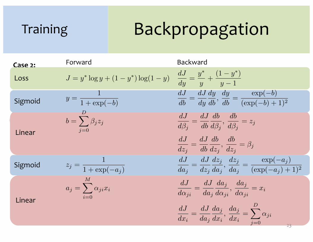
Case 2:Neural Network

…

…

Linear

Sigmoid

Linear

Sigmoid

Loss

Backpropagation

23

Training

Forward Backward

J = y� y + (1 � y�) (1 � y)dJ

dy=

y�

y+

(1 � y�)

y � 1

y =1

1 + (�b)

dJ

db=

dJ

dy

dy

db,

dy

db=

(�b)

( (�b) + 1)2

b =D�

j=0

�jzjdJ

d�j=

dJ

db

db

d�j,

db

d�j= zj

dJ

dzj=

dJ

db

db

dzj,

db

dzj= �j

zj =1

1 + (�aj)

dJ

daj=

dJ

dzj

dzj

daj,

dzj

daj=

(�aj)

( (�aj) + 1)2

aj =M�

i=0

�jixidJ

d�ji=

dJ

daj

daj

d�ji,

daj

d�ji= xi

dJ

dxi=

dJ

daj

daj

dxi,

daj

dxi=

D�

j=0

�ji

Backpropagation

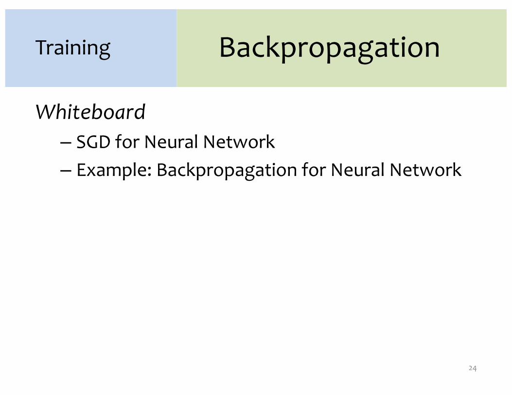
Whiteboard– SGD for Neural Network– Example: Backpropagation for Neural Network

24

Training

Backpropagation

25

Training

Backpropagation (Auto.Diff. - Reverse Mode)

Forward Computation1. Write an algorithm for evaluating the function y = f(x). The

algorithm defines a directed acyclic graph, where each variable is a node (i.e. the “computation graph”)

2. Visit each node in topological order. a. Compute the corresponding variable’s valueb. Store the result at the node

Backward Computation1. Initialize all partial derivatives dy/duj to 0 and dy/dy = 1.2. Visit each node in reverse topological order.

For variable ui = gi(v1,…, vN)a. We already know dy/duib. Increment dy/dvj by (dy/dui)(dui/dvj)

(Choice of algorithm ensures computing (dui/dvj) is easy)

Return partial derivatives dy/dui for all variables

A Recipe for Machine Learning

1. Given training data: 3. Define goal:

26

Background

2. Choose each of these:– Decision function

– Loss function

4. Train with SGD:(take small steps opposite the gradient)

Gradients

Backpropagation can compute this gradient! And it’s a special case of a more general algorithm called reverse-mode automatic differentiation that can compute the gradient of any differentiable function efficiently!

Summary

1. Neural Networks…– provide a way of learning features– are highly nonlinear prediction functions– (can be) a highly parallel network of logistic

regression classifiers– discover useful hidden representations of the

input2. Backpropagation…– provides an efficient way to compute gradients– is a special case of reverse-mode automatic

differentiation27

DEEP NETS

28

A Recipe for Machine Learning

1. Given training data: 3. Define goal:

29

Background

2. Choose each of these:– Decision function

– Loss function

4. Train with SGD:(take small steps opposite the gradient)

Goals for Today’s Lecture

1. Explore a new class of decision functions (Deep Neural Networks)

2. Consider variants of this recipe for training

Idea #1: No pre-training

30

Training

� Idea #1: (Just like a shallow network)� Compute the supervised gradient by backpropagation.� Take small steps in the direction of the gradient (SGD)

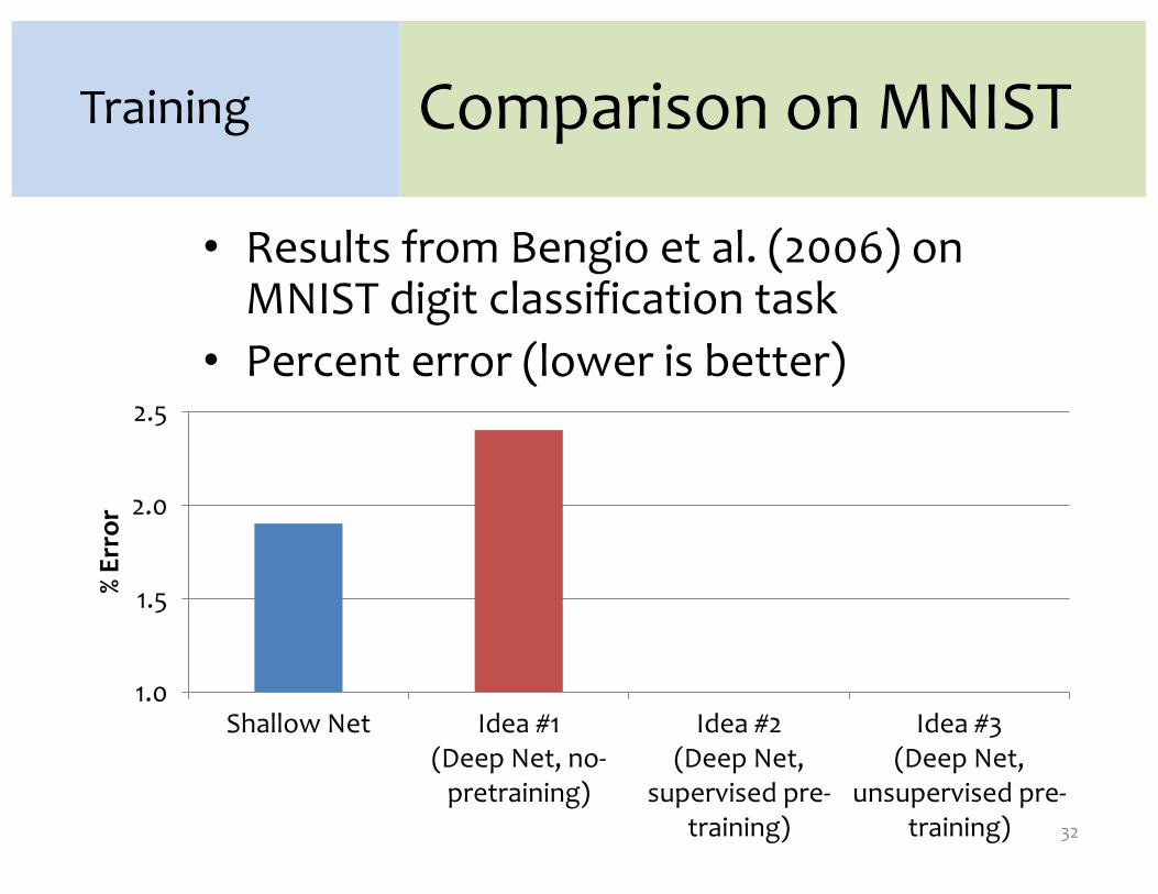
Comparison on MNIST

1.0

1.5

2.0

2.5

Shallow Net Idea #1(Deep Net, no-

pretraining)

Idea #2(Deep Net,

supervised pre-training)

Idea #3(Deep Net,

unsupervised pre-training)

% Er

ror

31

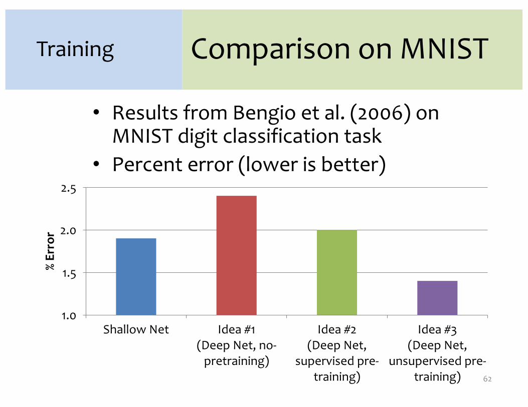
Training

• Results from Bengio et al. (2006) on MNIST digit classification task

• Percent error (lower is better)

Comparison on MNIST

1.0

1.5

2.0

2.5

Shallow Net Idea #1(Deep Net, no-

pretraining)

Idea #2(Deep Net,

supervised pre-training)

Idea #3(Deep Net,

unsupervised pre-training)

% Er

ror

32

Training

• Results from Bengio et al. (2006) on MNIST digit classification task

• Percent error (lower is better)

Idea #1: No pre-training

• What goes wrong?A. Gets stuck in local optima

• Nonconvex objective • Usually start at a random (bad) point in parameter space

B. Gradient is progressively getting more dilute• “Vanishing gradients”

33

Training

� Idea #1: (Just like a shallow network)� Compute the supervised gradient by backpropagation.� Take small steps in the direction of the gradient (SGD)

0.00.5

1.0

-20-15

-10-5

-20

-15

-10

-5

0

Problem A:Nonconvexity

• Where does the nonconvexity come from?• Even a simple quadratic z = xy objective is

nonconvex:

34

Training

z

xy

Problem A:Nonconvexity

• Where does the nonconvexity come from?• Even a simple quadratic z = xy objective is

nonconvex:

35

Training

0.00.5

1.0

-20 -15 -10 -5

-20

-15

-10

-5

0

z

xy

36

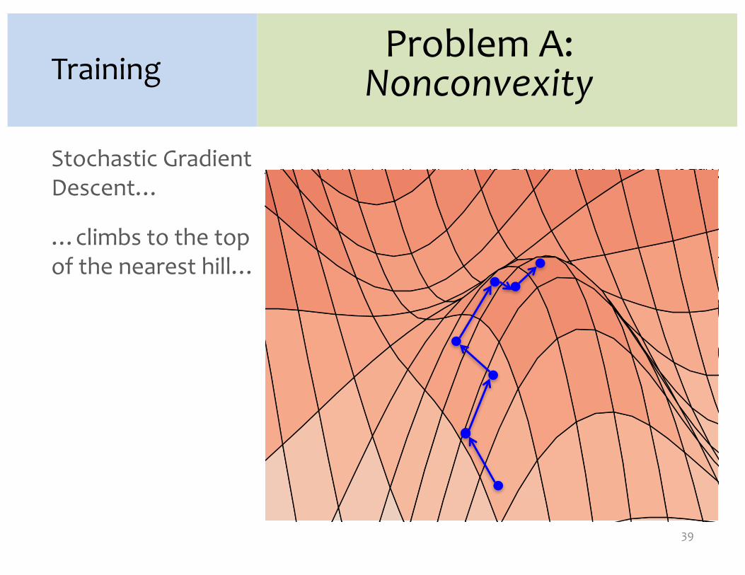
Stochastic GradientDescent…

…climbs to the top of the nearest hill…

Problem A:NonconvexityTraining

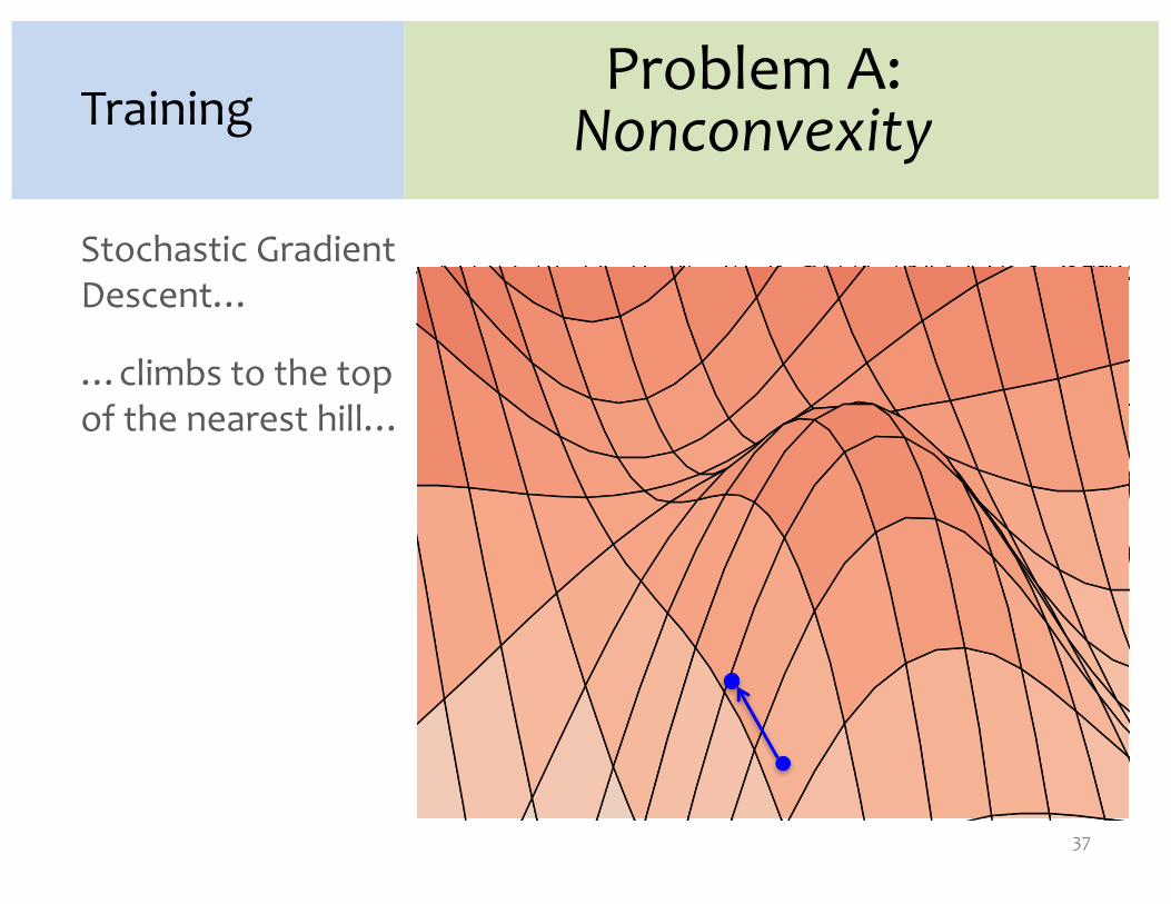
37

Stochastic GradientDescent…

…climbs to the top of the nearest hill…

Problem A:NonconvexityTraining

38

Stochastic GradientDescent…

…climbs to the top of the nearest hill…

Problem A:NonconvexityTraining

39

Stochastic GradientDescent…

…climbs to the top of the nearest hill…

Problem A:NonconvexityTraining

40

Stochastic GradientDescent…

…climbs to the top of the nearest hill…

…which might not lead to the top of the mountain

Problem A:NonconvexityTraining

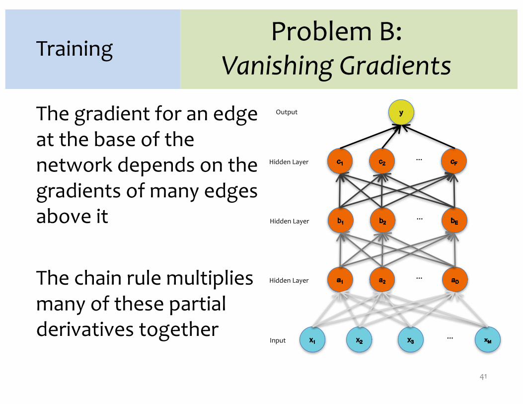
Problem B:Vanishing Gradients

The gradient for an edge at the base of the network depends on the gradients of many edges above it

The chain rule multiplies many of these partial derivatives together

41

Training

…

…Input

Hidden Layer

…Hidden Layer

…

Output

Hidden Layer

Problem B:Vanishing Gradients

The gradient for an edge at the base of the network depends on the gradients of many edges above it

The chain rule multiplies many of these partial derivatives together

42

Training

…

…Input

Hidden Layer

…Hidden Layer

…

Output

Hidden Layer

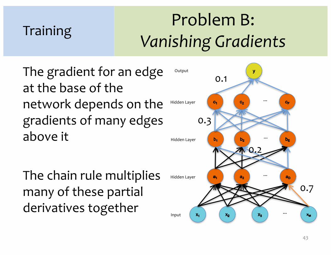
Problem B:Vanishing Gradients

The gradient for an edge at the base of the network depends on the gradients of many edges above it

The chain rule multiplies many of these partial derivatives together

43

Training

…

…Input

Hidden Layer

…Hidden Layer

…

Output

Hidden Layer

0.1

0.3

0.2

0.7

Idea #1: No pre-training

• What goes wrong?A. Gets stuck in local optima

• Nonconvex objective • Usually start at a random (bad) point in parameter space

B. Gradient is progressively getting more dilute• “Vanishing gradients”

44

Training

� Idea #1: (Just like a shallow network)� Compute the supervised gradient by backpropagation.� Take small steps in the direction of the gradient (SGD)

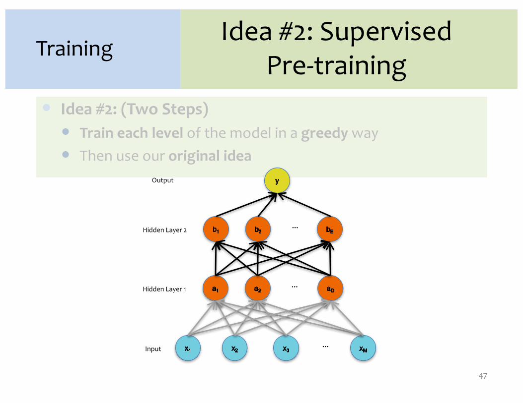
Idea #2: Supervised Pre-training

1. Supervised Pre-training– Use labeled data– Work bottom-up• Train hidden layer 1. Then fix its parameters.• Train hidden layer 2. Then fix its parameters.• …• Train hidden layer n. Then fix its parameters.

2. Supervised Fine-tuning– Use labeled data to train following “Idea #1”– Refine the features by backpropagation so that they become

tuned to the end-task45

Training

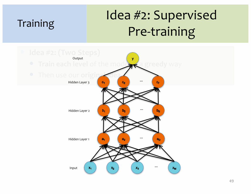
� Idea #2: (Two Steps)� Train each level of the model in a greedy way� Then use our original idea

Idea #2: Supervised Pre-training

46

Training

� Idea #2: (Two Steps)� Train each level of the model in a greedy way� Then use our original idea

…

…

Output

Input

Hidden Layer 1

� Idea #2: (Two Steps)� Train each level of the model in a greedy way� Then use our original idea

Idea #2: Supervised Pre-training

47

Training

…

…Input

Hidden Layer 1

…

Output

Hidden Layer 2

Idea #2: Supervised Pre-training

48

Training

� Idea #2: (Two Steps)� Train each level of the model in a greedy way� Then use our original idea

…

…Input

Hidden Layer 1

…Hidden Layer 2

…

Output

Hidden Layer 3

Idea #2: Supervised Pre-training

49

Training

� Idea #2: (Two Steps)� Train each level of the model in a greedy way� Then use our original idea

…

…Input

Hidden Layer 1

…Hidden Layer 2

…

Output

Hidden Layer 3

Comparison on MNIST

1.0

1.5

2.0

2.5

Shallow Net Idea #1(Deep Net, no-

pretraining)

Idea #2(Deep Net,

supervised pre-training)

Idea #3(Deep Net,

unsupervised pre-training)

% Er

ror

50

Training

• Results from Bengio et al. (2006) on MNIST digit classification task

• Percent error (lower is better)

Comparison on MNIST

1.0

1.5

2.0

2.5

Shallow Net Idea #1(Deep Net, no-

pretraining)

Idea #2(Deep Net,

supervised pre-training)

Idea #3(Deep Net,

unsupervised pre-training)

% Er

ror

51

Training

• Results from Bengio et al. (2006) on MNIST digit classification task

• Percent error (lower is better)

Idea #3: UnsupervisedPre-training

1. Unsupervised Pre-training– Use unlabeled data– Work bottom-up• Train hidden layer 1. Then fix its parameters.• Train hidden layer 2. Then fix its parameters.• …• Train hidden layer n. Then fix its parameters.

2. Supervised Fine-tuning– Use labeled data to train following “Idea #1”– Refine the features by backpropagation so that they become

tuned to the end-task52

Training

� Idea #3: (Two Steps)� Use our original idea, but pick a better starting point� Train each level of the model in a greedy way

The solution:Unsupervised pre-

training

53

…

…Input

Hidden Layer

Output

Unsupervised pre-training of the first layer: • What should it predict?• What else do we

observe? • The input!

This topology defines an Auto-encoder.

The solution:Unsupervised pre-

trainingUnsupervised pre-training of the first layer: • What should it predict?• What else do we

observe? • The input!

This topology defines an Auto-encoder.

54

…

…Input

Hidden Layer

…“Input” ’ ’ ’ ’

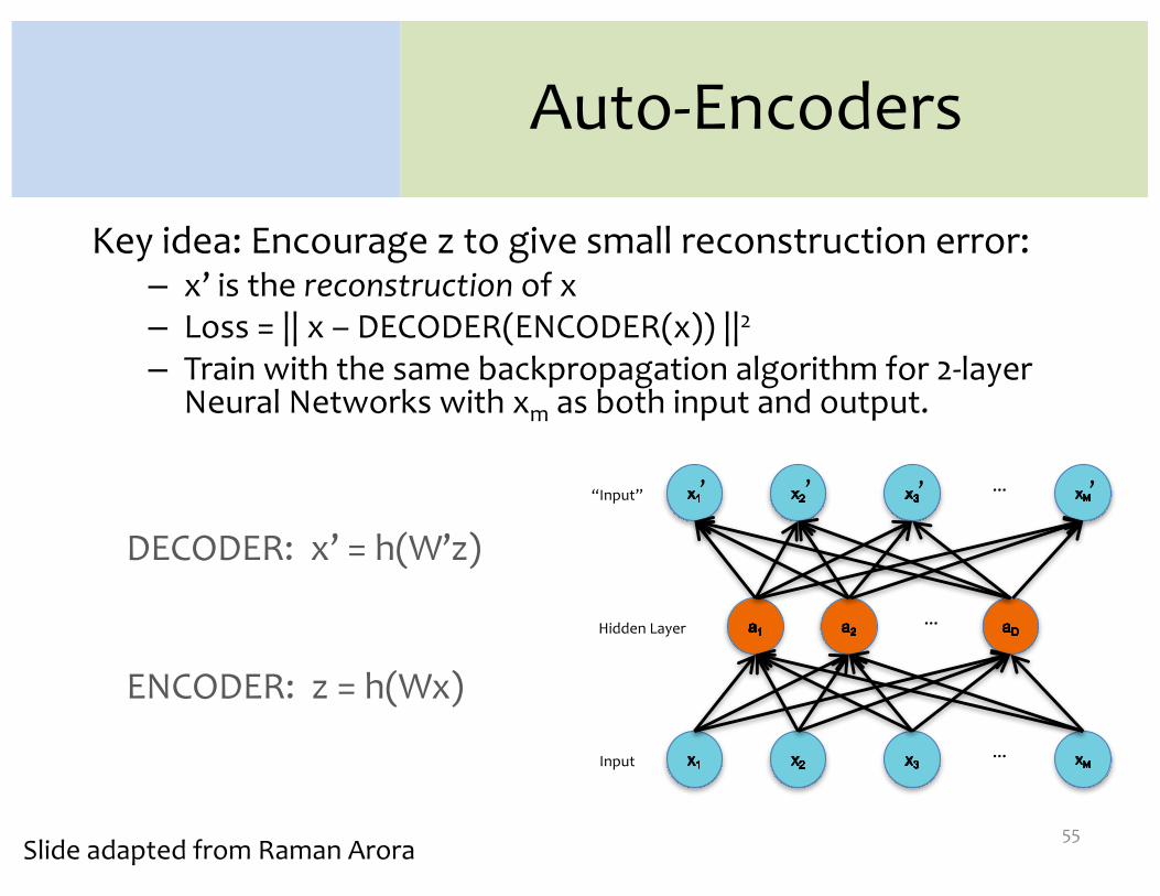
Auto-Encoders

Key idea: Encourage z to give small reconstruction error:– x’ is the reconstruction of x– Loss = || x – DECODER(ENCODER(x)) ||2

– Train with the same backpropagation algorithm for 2-layer Neural Networks with xm as both input and output.

55

…

…Input

Hidden Layer

…“Input” ’ ’ ’ ’

Slide adapted from Raman Arora

DECODER: x’ = h(W’z)

ENCODER: z = h(Wx)

The solution:Unsupervised pre-

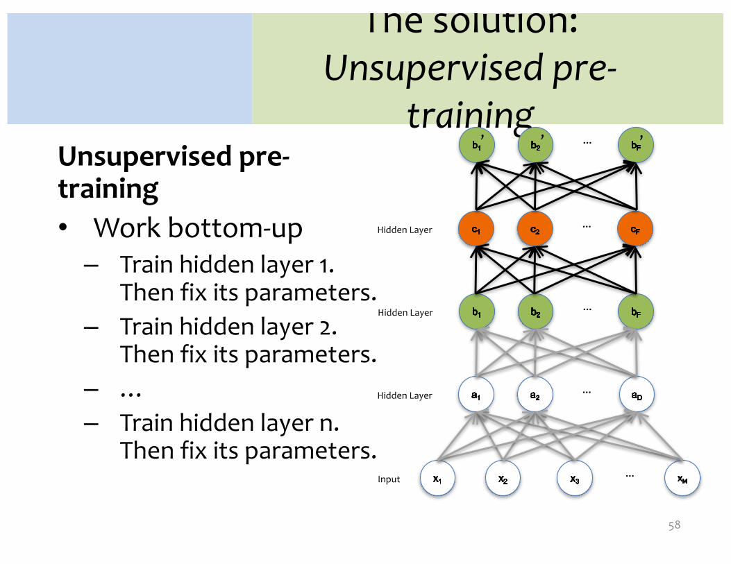
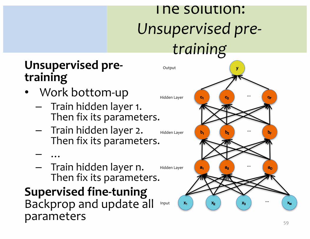
trainingUnsupervised pre-training• Work bottom-up– Train hidden layer 1.

Then fix its parameters.– Train hidden layer 2.

Then fix its parameters.– …– Train hidden layer n.

Then fix its parameters.

56

…

…Input

Hidden Layer

…“Input” ’ ’ ’ ’

The solution:Unsupervised pre-

trainingUnsupervised pre-training• Work bottom-up– Train hidden layer 1.

Then fix its parameters.– Train hidden layer 2.

Then fix its parameters.– …– Train hidden layer n.

Then fix its parameters.

57

…

…Input

Hidden Layer

…Hidden Layer

…’ ’ ’

The solution:Unsupervised pre-

trainingUnsupervised pre-training• Work bottom-up– Train hidden layer 1.

Then fix its parameters.– Train hidden layer 2.

Then fix its parameters.– …– Train hidden layer n.

Then fix its parameters.

58

…

…Input

Hidden Layer

…Hidden Layer

…Hidden Layer

…’ ’ ’

The solution:Unsupervised pre-

trainingUnsupervised pre-training• Work bottom-up– Train hidden layer 1.

Then fix its parameters.– Train hidden layer 2.

Then fix its parameters.– …– Train hidden layer n.

Then fix its parameters.Supervised fine-tuningBackprop and update all parameters

59

…

…Input

Hidden Layer

…Hidden Layer

…Hidden Layer

Output

Deep Network Training

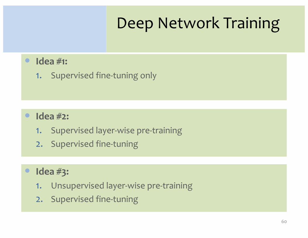
60

� Idea #3:1. Unsupervised layer-wise pre-training2. Supervised fine-tuning

� Idea #2:1. Supervised layer-wise pre-training2. Supervised fine-tuning

� Idea #1:1. Supervised fine-tuning only

Comparison on MNIST

1.0

1.5

2.0

2.5

Shallow Net Idea #1(Deep Net, no-

pretraining)

Idea #2(Deep Net,

supervised pre-training)

Idea #3(Deep Net,

unsupervised pre-training)

% Er

ror

61

Training

• Results from Bengio et al. (2006) on MNIST digit classification task

• Percent error (lower is better)

Comparison on MNIST

1.0

1.5

2.0

2.5

Shallow Net Idea #1(Deep Net, no-

pretraining)

Idea #2(Deep Net,

supervised pre-training)

Idea #3(Deep Net,

unsupervised pre-training)

% Er

ror

62

Training

• Results from Bengio et al. (2006) on MNIST digit classification task

• Percent error (lower is better)

Is layer-wise pre-training always necessary?

63

Training

In 2010, a record on a hand-writing recognition task was set by standard supervised backpropagation (our Idea #1).

How? A very fast implementation on GPUs.

See Ciresen et al. (2010)

Deep Learning

• Goal: learn features at different levels of abstraction

• Training can be tricky due to…– Nonconvexity– Vanishing gradients

• Unsupervised layer-wise pre-training can help with both!

64