Globalization and the Great Divergence

Globalization and the Great Divergence

Jeffrey G. Williamson Harvard University and the University of Wisconsin

Inaugural Lecture

Universitat Pompeu Fabra

October 8 2008

Motivation

In David Landes’ (1998) words, why is the Third World periphery in the South so poor, and the industrial OECD core in the North so rich?

The competing explanations or fundamentals:

Culture: Polyani 1944; Landes 1998; Clark 2007

Geography: Diamond 1997; Sachs 2000, 2001; Easterly & Levine 2003

Institutions: North & Weingast 1989; AJR 2001, 2002, 2005

Problems

Fundamentals don’t change very much over time.

So, what explains the timing of the great divergence between Core and Periphery? Why did the gap open so fast 1800-1913?

One possible explanation: the world was --

Closed and anti-global pre-1800

Open and pro-global 1800-1913

Closed and anti-global 1913-1950

Open and pro-global 1950-2008

Four Big Facts

Fact 1: Rise in the Core-Periphery Income Per

Capita Gap

The rise of the North-South gap

Rise in the Core-Periphery Income Per Capita Gap 1820-1998

0

2

4

6

8

10

12

14

1820 1870 1913 1950 1973 1998

WesternEurope/Africa

Western Europe/Asia

Western Europe/LatinAmerica

Parity

Source: Maddison (2001,

Table B-21)

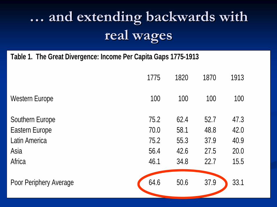
… and extending backwards with

real wages

Table 1. The Great Divergence: Income Per Capita Gaps 1775-1913

1775 1820 1870 1913

Western Europe 100 100 100 100

Southern Europe 75.2 62.4 52.7 47.3

Eastern Europe 70.0 58.1 48.8 42.0

Latin America 75.2 55.3 37.9 40.9

Asia 56.4 42.6 27.5 20.0

Africa 46.1 34.8 22.7 15.5

Poor Periphery Average 64.6 50.6 37.9 33.1

Four Big Facts


Capita Gap

Fact 2: De-Industrialization in the Poor Periphery

Do Industrial Countries Get Richer?

Current GDP per capita 1820-1950 and Industrialization 50 or 70 Years Before

Per Capita Levels of Industrialization 1750-1953

1750 1800 1860 1913 1953

European Core 8 8 17 45 90

Asian and Latin American Periphery 7 6 4 2 5

Ratio Core/Periphery 1.1 1.3 4.3 22.5 18

Source: Bairoch (1982, Table 4, p. 281). The European core contains: Austria-Hungary, Belgium,

France, Germany, Italy, Russia, Spain, Sweden, Switzerland, United Kingdom. The Asian and Latin

American periphery contains: China, India (plus Pakistan in 1953), Brazil and Mexico.

More de-industrialization figures

Textiles

Percent of Home Market Supplied by

Imports Domestic Industry

India 1833 5 95

India 1887 58-65 35-42

Ottoman 1820s 3 97

Ottoman 1870s 62-89 11-38

Mexico 1800s 25 75

Mexico 1879 40 60

Four possible causes of de-industrialization

in the Poor Periphery

● World market integration (e.g. globalization)

induces greater specialization (e.g. a new economic

order); implies tot improvement for periphery

● Rapid industrial productivity growth in Europe:

implies tot improvement for periphery

● Deterioration in industrial productivity and

competitiveness in periphery; implies no tot

improvement for periphery

● Improved productivity in primary product export

sector in periphery; implies no tot improvement for

periphery

Four Big Facts


Capita Gap

Fact 2: De-Industrialization in the Poor

Periphery

Fact 3: Secular Terms of Trade Boom and Bust

in the Periphery

The 18th c calm before the storm …

The 19th c storm …

Some more than others

Figure 4. The Poor Periphery: Net Barter Terms of Trade 1796-1913

0

50

100

150

200

250

1796 1802 1808 1814 1820 1826 1832 1838 1844 1850 1856 1862 1868 1874 1880 1886 1892 1898 1904 1910

Te

rms

of

Tra

de

Middle East

Latin America

Southeast Asia

European Periphery

South Asia

And the terms of trade bust, as seen

from Latin America 1811-1939 Figure 1

Latin American Terms of Trade 1811-1939

0

20

40

60

80

100

120

140

160

1811

1815

1819

1823

1827

1831

1835

1839

1843

1847

1851

1855

1859

1863

1867

1871

1875

1879

1883

1887

1891

1895

1899

1903

1907

1911

1915

1919

1923

1927

1931

1935

1939

Year

Px/

Pm

Average LA TOT Unadjusted

Average LA TOT Adjusted

Source: Unadjusted--Clingingsmith and Williamson (2004), Figure 9, based on data in Coatsworth and Williamson (2004a); Adjusted--see Appendix

1.

What caused the 120-year secular boom-

bust in terms of trade for primary-

product producers?

World market integration generated by a

world-wide transport revolution caused CPC,

lowered Pm and raised Px. Very fast initially,

then a slow-down to steady state.

First

The 19th Century Transport Revolution on Sea Lanes

And then a slow approach to steady state …

Figure 2.2: Real Global Freight Rate Index(1869-1997) (1884=1.00)

0.00

0.20

0.40

0.60

0.80

1.00

1.20

1.40

1870

-187

4

1875

-187

9

1880

-188

418

84

1885

-188

9

1890

-189

4

1895

-189

9

1900

-190

4

1905

-190

9

1910

-191

4

1915

-191

9

1920

-192

4

1925

-192

9

1930

-193

4

1935

-193

9

1940

-194

4

1945

-194

9

1950

-195

4

1955

-195

9

1960

-196

4

1965

-196

9

1970

-197

4

1975

-197

9

1980

-198

4

1985

-198

9

1990

-199

4

Second

Diffusion of the industrial revolution in core raised

GDP growth rates there, and thus in the derived

demand for luxury foodstuffs.

Growth rates of manufacturing were even greater

in core – since its share in GDP was rising, and

thus so too was derived demand for primary

product intermediates.

Manufacturing growth slowed down in core as

industrial transition was completed there, and

thus so too did the derived demand for primary

product intermediates.

Third

Manufacturing searched for new technologies

and synthetic products to save on or even

replace the increasingly expensive primary

products. It finally found them adding further

to the demand-led terms of trade bust.

Four Big Facts


Capita Gap


Periphery


in the Periphery

Fact 4: Terms of Trade Volatility Much Bigger

in the Periphery

Core vs Poor Periphery

Region Before 1820 1820-1870 1870-1913

United Kingdom 11.985 2.910 2.006

Average Periphery 6.460 9.176 7.089

European Periphery 4.036 10.720 7.058

Italy 0.922 19.003 11.214

Russia 3.226 10.722 6.104

Spain 7.959 6.472 6.023

Latin America 3.728 6.429 8.140

Argentina 4.409 6.961 8.303

Brazil N/A 2.174 10.283

Mexico 1.658 5.531 5.379

Middle East 2.902 13.611 7.316

Egypt 2.982 17.861 11.760

Ottoman Turkey 2.821 6.549 3.289

South Asia 11.876 9.628 5.364

Ceylon 17.860 7.590 7.532

India 5.891 11.666 3.196

Southeast Asia 7.788 6.977 7.303

Philippines 7.992 9.778 6.603

Siam 7.583 7.951 6.732

East Asia 15.554 10.527 4.952

China 15.554 19.752 4.311

Japan N/A 1.302 5.592

Table 3. Terms of Trade Volatility 1782-1913

Four Big Facts


Capita Gap


Periphery


in the Periphery

Fact 4: Terms of Trade Volatility Much Bigger

in the Periphery

One Big Question

Are the correlations spurious

or are they causal?

So, what about the theory,

and what about the magnitudes?

What’s the Impact of a Secular Improvement in the

Terms of Trade for a Primary Product Exporter?

Short Run: unambiguous income

increase Medium Run: unambiguous income increase

via resource allocation and specialization

response, e.g. de-industrialization

Long Run: ambiguous impact on growth due to

de-industrialization and the belief that industry

is a carrier of modern economic growth

Net Impact: theory ambiguous, history must

resolve the issue

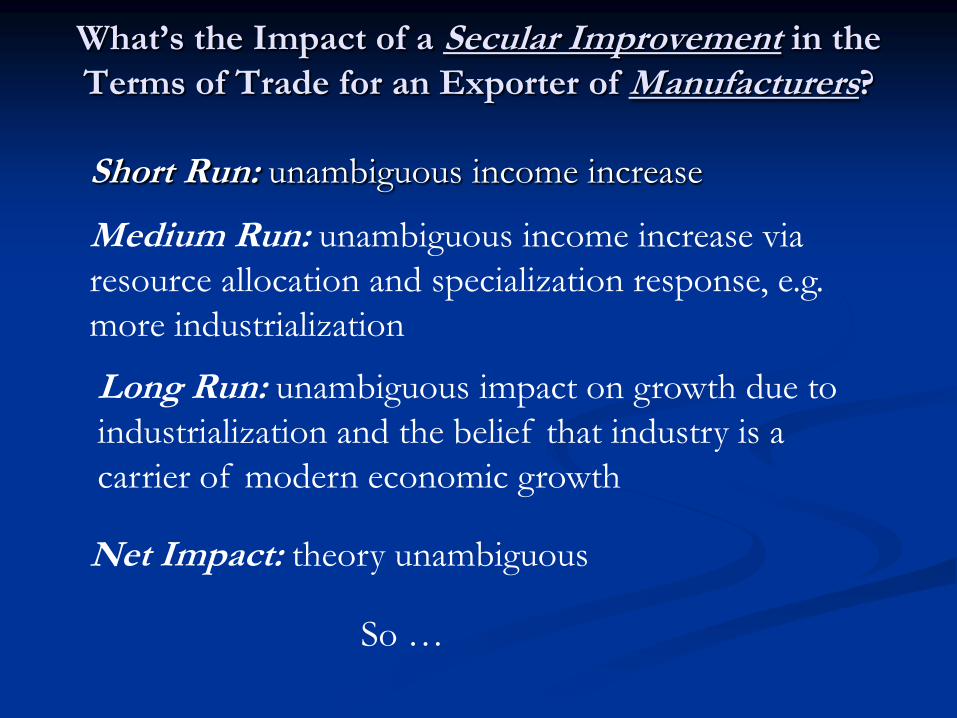
What’s the Impact of a Secular Improvement in the

Terms of Trade for an Exporter of Manufacturers?

Short Run: unambiguous income increase

Medium Run: unambiguous income increase via

resource allocation and specialization response, e.g.

more industrialization

Long Run: unambiguous impact on growth due to

industrialization and the belief that industry is a

carrier of modern economic growth

Net Impact: theory unambiguous

So …

What Should We Find in History?

Asymmetric impact

of secular terms of trade improvement

Core versus Periphery!

What’s the Impact of Terms of Trade

Volatility on the Exporter of Manufactures in

the Rich Core?

Exporters of manufactures in the rich core can

insure against price volatility cheaply since:

● they face well developed capital markets;

● governments have varied revenue sources;

● rich families can consumption smooth;

● they export many products, spreading risk;

● their export prices are less volatile.

What’s the Impact of Terms of Trade

Volatility on the Primary Product Exporter in

the Poor Periphery?

Poor primary product exporters cannot insure

against price volatility cheaply since:

● they face undeveloped capital markets;

● governments rely very heavily on import

duties and export taxes;

● poor families cannot consumption smooth;

● they export few products, so more vulnerable to

price shocks;

● their export prices are more volatile.

And risk-aversion begats lower accumulation!

So ….

What Should We Find In History?

Asymmetric impact

of terms of trade volatility

Core versus Periphery!

Identification Assumptions: Two Concerns

First

Was the terms of trade exogenous everywhere in

the periphery? Was every poor country a price

taker? No, but results are robust to exclusion of

suspected price-makers e.g.

● remove any with 33% of world exports of any

commodity: Australia, Brazil, Chile, China,

India, Philippines, Russia; same result

● plus, remove any with 25% of world exports of

any commodity: Argentina, Canada, Japan; same

result.

Second

Did some fundamental – institutions, geography or

culture -- drive both the choice of export product and

growth? Maybe, but so what?

● captured by country fixed effects, since export

“choice” was made long before 1870 and persisted

until 1939

● anyway, no correlation between price volatility and

institutional quality

A new historical database, annual, 35

countries, 1870-1939

6 Core industrial leaders: AH, Fr, Ger, It, UK, USA

8 European Periphery: Den, Grc, Nor, Port, Serb, Sp, Swe, Rus

8 Latin American Periphery: Arg, Brz, Col, Ch, Cuba, Mex, Per, Ur

10 Asia-MidEast: Bur, Cey, Egy, Ind, Indo, Jap, Phil, Siam, Turk

3 English-speaking European Offshoots: Aus, Can, NZ

Covers more than 85% of world population

and more than 95% of world GDP in 1914.

Results are insensitive to alternative Core

versus Periphery allocations.

Periphery Core

TOT Growth 0.05 0.63

[0.119] [0.251]**

TOT Volatility -0.08 0.02

[0.033]** [0.058]

Observations 167 32

R-squared 0.35 0.74

Decade Dummies Yes Yes

Country Dummies Yes Yes

Controls Yes Yes

Summary Statistics:

GDP Growth

1.05

[1.66]

1.59

[1.28]

TOT Growth -0.28 0.3

[1.46] [1.02]

TOT Volatility 8.8 6.82

[5.17] [4.86]

Impact on Growth:



Growth and the Terms of Trade 1870-1939

(Dependent variable: Decadal average GDP per capita growth)

Robust standard errors in

brackets

** significant at 5%

Periphery Core


[0.119] [0.251]**


[0.033]** [0.058]

Observations 167 32

R-squared 0.35 0.74

Decade Dummies Yes Yes

Country Dummies Yes Yes

Controls Yes Yes

Summary Statistics:

GDP Growth

1.05

[1.66]

1.59

[1.28]

TOT Growth -0.28 0.3

[1.46] [1.02]

TOT Volatility 8.8 6.82

[5.17] [4.86]

Impact on Growth:



Growth and the Terms of Trade 1870-1939

(Dependent variable: Decadal average GDP per capita growth)

Robust standard errors

in brackets

** significant at 5%

Note:

Percentage point

impact of 1 st. dev.

change

What About pre-1870 History?

The data aren’t sufficient to estimate impact

as we did for 1870-1938.

But terms of trade volatility was even bigger

pre-1870 than post-1870, so bigger negative

impact on growth if the post-1870 impact

conditions also held for the pre-1870 period.

Core vs Poor Periphery

Region Before 1820 1820-1870 1870-1913

United Kingdom 11.985 2.910 2.006

Average Periphery 6.460 9.176 7.089

European Periphery 4.036 10.720 7.058

Italy 0.922 19.003 11.214

Russia 3.226 10.722 6.104

Spain 7.959 6.472 6.023

Latin America 3.728 6.429 8.140

Argentina 4.409 6.961 8.303

Brazil N/A 2.174 10.283

Mexico 1.658 5.531 5.379

Middle East 2.902 13.611 7.316

Egypt 2.982 17.861 11.760

Ottoman Turkey 2.821 6.549 3.289

South Asia 11.876 9.628 5.364

Ceylon 17.860 7.590 7.532

India 5.891 11.666 3.196

Southeast Asia 7.788 6.977 7.303

Philippines 7.992 9.778 6.603

Siam 7.583 7.951 6.732

East Asia 15.554 10.527 4.952

China 15.554 19.752 4.311

Japan N/A 1.302 5.592

Table 3. Terms of Trade Volatility 1782-1913

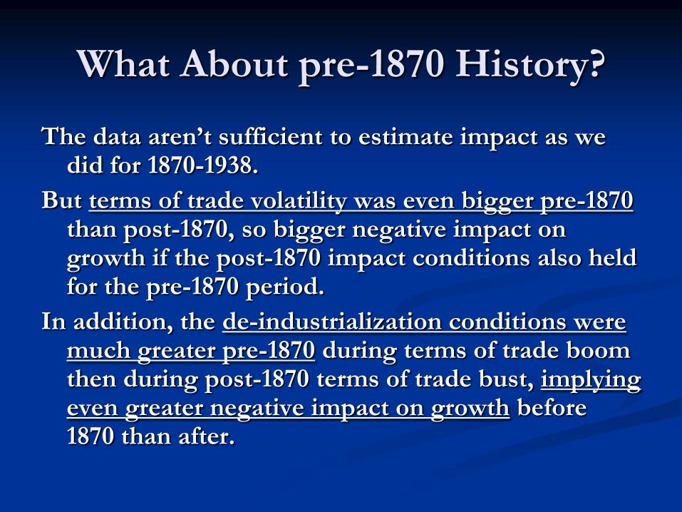
What About pre-1870 History?

The data aren’t sufficient to estimate impact as we did for 1870-1938.

But terms of trade volatility was even bigger pre-1870 than post-1870, so bigger negative impact on growth if the post-1870 impact conditions also held for the pre-1870 period.

In addition, the de-industrialization conditions were much greater pre-1870 during terms of trade boom then during post-1870 terms of trade bust, implying even greater negative impact on growth before 1870 than after.

Reminder: Terms of trade boom

versus bust (in Latin America) Figure 1

Latin American Terms of Trade 1811-1939

0

20

40

60

80

100

120

140

160

1811

1815

1819

1823

1827

1831

1835

1839

1843

1847

1851

1855

1859

1863

1867

1871

1875

1879

1883

1887

1891

1895

1899

1903

1907

1911

1915

1919

1923

1927

1931

1935

1939

Year

Px/

Pm

Average LA TOT Unadjusted

Average LA TOT Adjusted

Source: Unadjusted--Clingingsmith and Williamson (2004), Figure 9, based on data in Coatsworth and Williamson (2004a); Adjusted--see Appendix

1.

Bottom Lines

● Did globalization experience contribute to the Great

Divergence before 1940? Absolutely!

● How much of the gap in growth rates between core

and periphery 1870-1940 was explained by different tot

growth and volatility impact? Big: a third to a half.

● Would we expect the same tot impact pre-1870?

Bigger: secular tot boom, not bust, and tot volatility at

least as big.

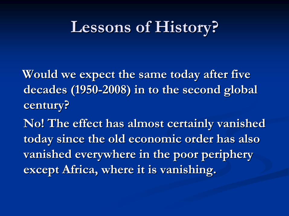
Lessons of History?

Would we expect the same today after five

decades (1950-2008) in to the second global

century?

No! The effect has almost certainly vanished

today since the old economic order has also

vanished everywhere in the poor periphery

except Africa, where it is vanishing.

Many thanks!

Globalization and the Great Divergence

Documents

Transcript of Globalization and the Great Divergence