Trade, Technology and the Great Divergence

Trade, Technology and the Great Divergence∗

Kevin H. O’Rourke, Ahmed S. Rahman, and Alan M. Taylor

March 2016

Abstract

This paper develops a model that captures the key features of the Industrial Revolution and

the Great Divergence between the industrializing “North” and the lagging “South.” Why

did North-South divergence occur so dramatically during the late 19th Century, rather

than at the outset of the Industrial Revolution? Further, why did some of these same

Southern economies undergo rapid convergence to Northern incomes starting in the mid-

20th century? To answer these questions we construct a trade/growth model that includes

both endogenous biased technologies and intercontinental trade. The Industrial Revolution

began as a sequence of unskilled-labor-intensive innovations which initially incited fertility

increases and limited human capital formation in both the North and the South. However,

the subsequent co-evolution of trade and local technological growth fostered an inevitable

divergence in living standards — the South increasingly specialized in production that

worsened its terms of trade and spurred even greater fertility increases and educational

declines. Local biased technological changes in both regions only reinforced this pattern, but

as knowledge became more globalized and diffused from the North to the South this pattern

reversed. The model highlights how interactions between trade-induced specialization and

technological forces help us understand divergence and convergence patterns in history.

• Keywords: Industrial Revolution, unified growth theory, endogenous growth, demog-

raphy, skill premium, Great Divergence

• JEL Codes: O, F, N

∗Preliminary draft. Please do not quote.

1 Introduction

The last two centuries have witnessed dramatic changes in the global distribution of income

and population. At the dawn of the Industrial Revolution, living standards between the richest

and poorest economies of the world were roughly 2 to 1. With industrialization came both income

and population growth in a few core countries. But massive divergence in living standards across

the globe did not take place until the latter half of the 19th century, the time when the first great

era of globalization started to take shape. Today the gap between material living standards in

the richest and poorest economies of the world is of the order of 30 or 40 to 1, in large part due to

the events of the 19th century. It seems an interesting coincidence then that such unprecedented

growth in inter-continental commerce (conceivably creating a powerful force for convergence by

exploiting comparative advantages and facilitating flows of knowledge) coincided so precisely with

an unprecedented divergence in living standards across the world. Why did incomes diverge just

as the world became flatter? This paper argues that trade and technological growth patterns

together sowed the seeds of divergence, contributing enormously to today’s great wealth disparity.

Some important “stylized facts” from economic history motivate our theory. One concerns

the nature of industrialization itself - technological change was unskilled-labor-intensive during

the early Industrial Revolution but became relatively skill-intensive during the late nineteenth

century. For example, the cotton textile industry, which along with metallurgy was at the heart of

the early Industrial Revolution, was able to employ large numbers of unskilled and uneducated

workers with minimal supervision, thus diminishing the relative demand for skilled labor and

education (Galor 2005; Clark 2007). By the 1850’s, however, two major changes had occurred —

technological growth became much more widespread, and it became far more skill-using (Mokyr

2002).

Another factor of great importance was the rising role of international trade in the world

economy. Inter-continental commerce between “western” economies and the rest of the world

(what we might mildly mislabel as “North-South” trade) grew dramatically in the second half of

the 19th century. By the 1840s steam ships were faster and more reliable than sailing ships, but

their high coal consumption limited how much cargo they could transport; consequently only very

light and valuable freight was shipped (O’Rourke and Williamson 1999). But by 1870 a number

of innovations dramatically reduced the cost of steam ocean transport, and real ocean freight

rates fell by nearly 35% from 1870 to 1910 (Clark and Feenstra 2003). By 1900 the economic

centers of the “South” such as Alexandria, Bombay and Shanghai were fully integrated into

the British economy, both in terms of transport costs and capital markets (Clark 2007). Thus,

while the British economy remained relatively closed during the first stages of the Industrial

Revolution (1750-1850), it became dramatically more open economy towards certain Southern

regions during the latter stages of industrialization (1850-1910).

We develop a model with a number of key features mimicking these historical realities. The

1

first key feature of the model is that we endogenize the direction and extent of technological

change in both regions. Technologies are sector specific, and sectors have different degrees of skill

intensity. Following the endogenous growth literature, we allow potential innovators to observe

the employment of factors in different sectors, and tailor their research efforts towards particular

sectors. Thus the scope and direction of innovation will depend on each region’s employment and

demography. The model is also flexible enough to allow for different technological environments,

such as the potential for the South to adopt Northern technologies, or for the South to develop

technologies themselves.

The second key feature is that we endogenize demography itself. More specifically, we allow

households to make education and fertility decisions based on market wages for skilled and

unskilled labor. The method is similar to other endogenous demography models where households

face a quality/quantity tradeoff with respect to their children. Thus, when the premium for skilled

labor rises families choose to have fewer but better educated children.

The final feature is that we allow for burgeoning trade between the North and the South.

During the initial stages of industrialization, trade is not possible due to prohibitively high

transport costs. These costs however exogenously decrease over time; at a certain point trade

becomes feasible, at which time the South exchanges labor-intensive products for the North’s

skill-intensive products. At this stage development paths begin to diverge - the North increasingly

specializes in skilled production while the South specializes in unskilled production.

With this basic setup, we simulate the model to roughly capture the main features of his-

torical industrialization and divergence between the North and the South. Because of the great

abundance of unskilled labor in the world before any industrialization, innovators first develop

unskilled-intensive technologies. Thus early industrialization is characterized by unskilled-labor-

intensive technological growth and population growth both in the North and the South; conse-

quently living standards in the two regions do not diverge during this time. Once trade becomes

possible, however, the North starts specializing in skill-intensive innovation and production.

This induces a demographic transition of falling fertility and rising education rates in the North.

The South on the other hand specializes in unskilled-labor-intensive production, inducing both

unskilled-labor-intensive technological growth and further population growth. This population

divergence fosters a deterioration in the South’s terms of trade, forcing the South to produce

more and more primary commodities and generating even more fertility increases (Figure 1).

Thus the South’s static gains from trade become a dynamic impediment to prosperity, and living

standards between the two regions diverge dramatically.

We can also demonstrate that this divergence can reverse when technologies are allowed to

flow from the North to the South (instead of being developed locally). In a more technologically

integrated world, we show that trade need not foster divergence, at least in the longer run.

2

Figure 1: Relative Price of Primary Products According to Lewis and Prebisch 1870-1950 (1912

= 100)

source: Hadass and Williamson (2003)

3

Alternative Stories of Divergence

We argue that analyzing the interactions between the North and the South, and between

trade and technological flows, is critical to understanding both the Industrial Revolution and

the Great Divergence. Many explanations of divergence rely on institutional differences between

regions of the world (North and Thomas 1973, Acemoglu et al. 2001, 2005). From this perspective

economic growth is a matter of establishing the right “rules of the game,” and underdevelopment

is simply a function of some form of institutional pathology. Our model implicitly assumes

that the institutional prerequisites for technological progress are in place. It goes on to make

the important point, however, that interactions between regions are an independent source of

potential divergence and convergence. It would be a mistake to think of differential growth

patterns as having been solely generated by institutional differences in economies operating in

isolation from each other.

Another potential explanation for the divergence is that peripheral countries were specializing

in inherently less-productive industries (Galor and Mountford 2006, 2008). But this is not

very convincing - so called low-technology sectors such as agriculture enjoyed large productivity

advances during the early stages of the Industrial Revolution (Bekar and Lipsey 1997, Clark

2007). And in the twentieth century, developing countries specialized in textile production which

had experienced massive technological improvements more than a century before.

A related puzzle is the scale of the developing world. If fully one third of the world had

become either Indian or Chinese by the twentieth century (Galor and Mountford 2002), why

were Indians and Chinese not wealthier? After all, most semi-endogenous and endogenous growth

theories have some form of scale effect, whereby large populations can spur innovation (Acemoglu,

forthcoming).1 Any divergence story that focuses on the explosive population expansion in

peripheral economies faces this awkward implication from the canonical growth literature.

Relation to Galor and Mountford’s “Trade and the Great Divergence”

The paper presented here relates most closely and obviously to Oded Galor and Andrew

Mountford’s theoretical works on the Great Divergence (Galor and Mountford 2006, 2008)

(henceforward ‘GM’). These papers similarly suggest that the South’s specialization in unskilled-

intensive production stimulated fertility increases which lowered per capita living standards.

However, our narrative of the North’s launching into modernity and the South’s vicious cycle of

underdevelopment is distinct in a number of ways.

1More specifically, in such seminal endogenous growth models as Romer (1986, 1990), Segerstrom, Anant and

Dinopolous (1990), Aghion and Howitt (1992), and Grossman and Helpman (1991), a larger labor force implies

faster growth of technology. In ”semi-endogenous” growth models such as Jones (1995), Young (1998), and Howitt

(1999), a larger labor force implies a higher level of technology.

4

The first involves the nature of trade. Since we are concerned with an era with limited North-

South exchanges of differentiated products and little intra-industry trade, trade is best modeled

as Ricardian (based on productivity differences) or Hecksher-Ohlin (based on factor differences)

in nature.2 GM use the former approach, while we use both. Such a hybrid trade model seems

most appropriate to us given the rather large North-South differences in both technologies and

factor endowments during the period we study.

Second, we endogenize both the scope and the direction of technological progress in both

regions. GM make assumptions concerning the timing and speed of technological growth which

they claim are “consistent with historical evidence.” Specifically, they assume that 1) modern-

ization either in agriculture or in manufacturing is not initially feasible, 2) modernization occurs

first in the agricultural sector, and 3) growth in industrial-sector productivity is faster than

growth in agricultural-sector productivity. Compelling as these assumptions seem to us, they

are not universally shared.3

Finally, rather than suddenly open up the North and South to trade, we allow for gradual

increases in North-South commerce. The British economy (and other Western economies) pre-

sumably did not undergo a discontinuous switch from a closed to an open state, and we thus

assume continuously declining transport costs. We suggest that the timing of globalization mat-

ters for the story of divergence.

These key differences allow us to infer something that is somewhat under-explored in GM

- growth in trade and technologies jointly created the dramatic divergence in living standards

between the North and the South. More specifically, while the South’s specialization in agri-

culture and low-end manufacturing allowed for plenty of technological advances in these areas,

these did not help the South keep up with the North for two reasons. One is that they fostered

fertility increases similar to the process outlined in GM. The other is that the South’s terms

of trade deteriorated over time. As the South grew in population it made up a larger share of

the world population, and thus flooded the world markets with its primary products. Northern

skill-intensive products became relatively scarcer, and thus fetched higher prices. The South had

to provide more and more primary products to buy the same amount of high-end products; this

served to raise fertility rates even more. This mechanism, absent in GM’s work, suggests that

productivity growth (and the scale that generated this growth) could not salvage the South; in

fact it contributed to its relative decline.

2We know that Heckscher-Ohlin trade was important during the 19th century since commodity price conver-

gence induced factor price convergence during this period (O’Rourke and Williamson 1994; O’Rourke, Taylor

and Williamson 1996; O’Rourke and Williamson 1999, Chapter 4). And Mitchener and Yan (2010) suggest that

unskilled-labor abundant China exported more unskilled-labor-intensive goods and imported more skill-intensive

goods from 1903 to 1928, consistent with such a trade model.3See for example Temin (1997) who argues that the British Industrial Revolution saw broad-based technological

change affecting all industries.

5

Finally, we provide a potential mechanism for how some regions were able to reverse this

divergence, even as trade costs continued to fall. If we allow the South to adopt from the world

technology frontier (instead of developing their own technologies locally), regions can break

the specialization patterns of the late 19th century and converge to Northern living standards.

We show that both trade and technological factors worked in tandem to help shape the global

distribution of income we see today.

2 Production with Given Technologies and Factors

We now sketch out a model that we will use to describe both a northern economy and a

southern economy (superscripts denoting region are suppressed for the time being).

Total production for a region is given by:

Y =(α

2yσ−1σ

1 + (1− α)yσ−1σ

2 +α

2yσ−1σ

3

) σσ−1

(1)

where α ∈ [0, 1] and σ ≥ 0. σ is the elasticity of substitution among intermediate goods y1, y2,

and y3. The production of these goods are given by:

y1 = A1L1 (2)

y1 = A2Lγ2H

1−γ2 (3)

y3 = A3H3 (4)

where A1, A2 and A3 are the technological levels of sectors 1, 2, and 3, respectively.4 These

technological levels in turn are represented by a series of sector-specific machines. Specifically,

A1 =

∫ N1

0

(x1 (j)

L1

)αdj (5)

A2 =

∫ N2

0

(x2 (j)

Lγ2H1−γ2

)αdj (6)

A3 =

∫ N3

0

(x3 (j)

H3

)αdj (7)

4Thus sectors vary by skill -intensity. While our interest is mainly in the “extreme” sectors (1 and 3), we

require an intermediate sector so that production of intermediate goods are determined both by relative prices

and endowments, and not pre-determined solely by endowments of L and H. This will be important when we

introduce trade to the model.

6

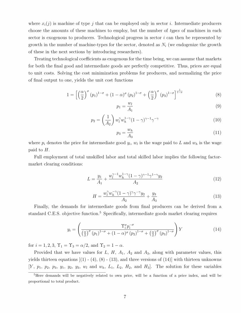
where xi(j) is machine of type j that can be employed only in sector i. Intermediate producers

choose the amounts of these machines to employ, but the number of types of machines in each

sector is exogenous to producers. Technological progress in sector i can then be represented by

growth in the number of machine-types for the sector, denoted as Ni (we endogenize the growth

of these in the next sections by introducing researchers).

Treating technological coefficients as exogenous for the time being, we can assume that markets

for both the final good and intermediate goods are perfectly competitive. Thus, prices are equal

to unit costs. Solving the cost minimization problems for producers, and normalizing the price

of final output to one, yields the unit cost functions

1 =[(α

2

)σ(p1)

1−σ + (1− α)σ (p2)1−σ +

(α2

)σ(p3)

1−σ] 1

1−σ(8)

p1 =wlA1

(9)

p2 =

(1

A2

)wγl w

1−γh (1− γ)γ−1γ−γ (10)

p3 =whA3

(11)

where pi denotes the price for intermediate good yi, wl is the wage paid to L and wh is the wage

paid to H.

Full employment of total unskilled labor and total skilled labor implies the following factor-

market clearing conditions:

L =y1A1

+wγ−1l w1−γ

h (1− γ)γ−1γ1−γy2A2

(12)

H =wγl w

−γh (1− γ)γγ−γy2

A2

+y3A3

(13)

Finally, the demands for intermediate goods from final producers can be derived from a

standard C.E.S. objective function.5 Specifically, intermediate goods market clearing requires

yi =

(Υσi p

−σi(

α2

)σ(p1)

1−σ + (1− α)σ (p2)1−σ +

(α2

)σ(p3)

1−σ

)Y (14)

for i = 1, 2, 3, Υ1 = Υ3 = α/2, and Υ2 = 1− α.

Provided that we have values for L, H, A1, A2 and A3, along with parameter values, this

yields thirteen equations [(1) - (4), (8) - (13), and three versions of (14)] with thirteen unknowns

[Y , p1, p2, p3, y1, y2, y3, wl and wh, L1, L2, H2, and H3]. The solution for these variables

5Here demands will be negatively related to own price, will be a function of a price index, and will be

proportional to total product.

7

constitutes the solution for the static model in the case of exogenously determined technological

and demographic variables.

3 Endogenizing Technologies in Both Regions

In this section we describe how innovators in both the North and (potentially) the South en-

dogenously develop new technologies. In general, modeling purposive research and development

effort is challenging when prices and factors change over time. This is because it is typically

assumed that the gains from innovation will flow to the innovator throughout his lifetime, and

this flow will often depend on the price of the product being produced and the factors required for

production at each moment in time.6 If prices and factors are constantly changing (as they will

in any economy where trade barriers fall gradually or factors evolve endogenously), a calculation

of the true discounted profits from an invention may be impossibly complicated.

To avoid such needless complication but still gain from the insights of endogenous growth

theory, we assume that the gains from innovation last one time period only. More specifically,

technological progress is sector-specific, and comes about though increases in the varieties of ma-

chines employed in each sector. New varieties of machines are developed by profit-maximizing

inventors, who monopolistically produce and sell the machines to competitive producers of the

intermediate goods y1, y2 or y3. However, we assume that the blueprints to these machines

become public knowledge the time period after the machine is invented, at which point these

machines become old and are competitively produced and sold.7 Thus while we need to distin-

guish between old and new sector-specific machines, we avoid complicated dynamic programming

problems inherent in multiple-period profit streams.8

Thus, we can re-define sector-specific technological levels given by (5) - (7) as a series of both

old and new machines at time t (once again suppressing region superscripts) as:

A1,t =

(∫ N1,t−1

0

x1,old(j)αdj +

∫ N1,t

N1,t−1

x1,new(j)αdj

)(1

L1

)α

A2,t =

(∫ N2,t−1

0

x2,old(j)αdj +

∫ N2,t

N2,t−1

x2,new(j)αdj

)(1

Lγ2H1−γ2

)α6For example, the seminal Romer (1990) model describes the discounted present value of a new invention as

a positive function of L− LR, where L is the total workforce and LR are the number of researchers. Calculating

this value function is fairly straight-forward if labor supplies of production workers and researchers are constant.

If they are not, however, calculating the true benefits to the inventor may be difficult.7Here one can assume either that patent protection for intellectual property lasts one time period, or that it

takes one time period for potential competitors to reverse-engineer the blueprints for new machines.8See Rahman (2013) for more discussion of this simplifying (but arguably more realistic) assumption.

8

A3,t =

(∫ N3,t−1

0

x3,old(j)αdj +

∫ N3,t

N3,t−1

x3,new(j)αdj

)(1

H3

)αwhere xi,old are machines invented before t, and xi,new are machines invented at t. Thus in each

sector i there are Nt−1 varieties of old machines that are competitively produced, and there

are Nt −Nt−1 varieties of new machines that are monopolistically produced (again, suppressing

country subscripts).

Next, we must describe producers of intermediate goods in each region. These three different

groups of producers each separately solve the following maximization problems:

Sector 1 producers: max[L1,x1(j)] p1y1 − wlL1 −∫ N1

0χ1(j)x1(j)dj

Sector 2 producers: max[L2,H2,x2(j)] p2y2 − wlL2 − whH2 −∫ N2

0χ2(j)x2(j)dj

Sector 3 producers: max[H3,x3(j)] p3y3 − whH3 −∫ N3

0χ3(j)x3(j)dj

where χi(j) is the price of machine j employed in sector i. For each type of producer, solving

the maximization problem with respect to machine j yields a solution for machine demand:

x1(j) = χ1(j)1

α−1 (αp1)1

1−α L1 (15)

x2(j) = χ2(j)1

α−1 (αp2)1

1−α Lγ2H1−γ2 (16)

x3(j) = χ3(j)1

α−1 (αp3)1

1−α H3 (17)

New machine producers, having the sole right to produce the machine, set the price of their

machines to maximize instantaneous profit. This price will be a constant markup over the

marginal cost of producing a machine. Assuming that the cost of making a machine is unitary

implies that χ1(j) = χ2(j) = χ3(j) = χ = 1/α for new machines. Thus, substituting in this

mark-up price, and realizing that instantaneous profits are (1/α)− 1 multiplied by the number

of new machines sold, instantaneous revenues by new machine producers are given by:

π1 =

(1− αα

)α

21−α (p1)

11−α L1 (18)

π2 =

(1− αα

)α

21−α (p2)

11−α Lγ2H

1−γ2 (19)

π3 =

(1− αα

)α

21−α (p3)

11−α H3 (20)

9

Old machines, on the other hand, are competitively produced; competition will drive the price

of all these machines down to marginal cost, so that χ1(j) = χ2(j) = χ3(j) = χ = 1 for all old

machines. Sectoral productivities can then be expressed simply as a combination of old and

new machines demanded by producers. Plugging in the appropriate machine prices into our

machine demand expressions (15) - (17), and plugging these machine demands into our sectoral

productivities, we can express these productivities as:

A1 =(N1,t−1 + α

α1−α (N1,t −N1,t−1)

)(αp1)

α1−α (21)

A2 =(N2,t−1 + α

α1−α (N2,t −N2,t−1)

)(αp2)

α1−α (22)

A3 =(N3,t−1 + α

α1−α (N3,t −N3,t−1)

)(αp3)

α1−α (23)

Thus, if we have given to us the number of old and new machines that can be used in each

sector (the evolution of these are described in section 5.1) , we can simultaneously solve equations

(8) - (14) and (21) - (23) to solve for prices, wages, intermediate goods and technological levels

for a hypothetical economy. Our next goal is to also endogenize the levels of skilled and unskilled

labor in this hypothetical economy.

4 Endogenizing Population and Labor-Types in Both Re-

gions

We now introduce an over-lapping generations framework, where individuals in each region

live for two time periods. In their youths individuals work as unskilled workers; this income

is consumed by their parents. When they become adults, individuals decide whether or not to

expend a fixed resource cost to become a skilled worker. Adults also decide how many of their

own children to have, who earn unskilled income for the adults. Adults however are required to

forgo some income for child-rearing.

Specifically, an adult i’s objective is to maximize current-period income. If an adult chooses to

remain an unskilled worker (L), she aims to maximize Il with respect to her number of children,

where

Il = wl + nlwl − wlλ(nl − 1)φ (24)

wl is the unskilled labor wage, nl is the number of children that the unskilled adult has, and

λ > 0 and φ > 1 are constant parameters that affect the opportunity costs to child-rearing. Note

10

that costs include a nl − 1 term to ensure that at least replacement fertility is maintained.

If an adult chooses to spend resources to become a skilled worker, she instead maximizes Ih

with respect to her number of children, where

Ih = wh + nhwl − whλ(nh − 1)φ − τi (25)

wh is the skilled labor wage, nh is the number of children that the skilled adult has, and τi is the

resources she must spend to become skilled.

The first order conditions for each of these groups give us the optimal fertility for each group.

For analytical convenience we will solve for fertility in excess of replacement, n∗l and n∗

h:

n∗l = nl − 1 = (φλ)

11−φ (26)

n∗h = nh − 1 =

(whwlφλ

) 11−φ

(27)

Note that with wh > wl, the optimal fertility for a skilled worker is always smaller than that

for an unskilled worker (this is simply because the opportunity costs of child-rearing are larger for

skilled workers). Also note that the fertility for unskilled workers is constant, while the fertility

for skilled workers falls with increases in the skill premium.

Finally, assume that τ varies across adults. The resource costs necessary to acquire an educa-

tion can vary across individuals for many reasons, including differing incomes, access to schooling,

or innate abilities. Say τi is uniformly distributed across [0, b], where b > 0. An individual i who

draws a particular τi will choose to become a skilled worker only if her optimized income as a

skilled worker will be larger than her optimized income as an unskilled worker. Let us call τ ∗

the threshold cost to education; this is the education cost where the adult is indifferent between

becoming a skilled worker or remaining an unskilled worker. Solving for this, we get

τ ∗ = wh + n∗hwl − whλn∗φ

h − wl − n∗lwl + wlλn

∗φl (28)

Only individuals whose τi fall below this level will opt to become skilled.

Figure 2 illustrate optimal fertility rates for two individuals - one with a relatively high τ and

one with a relatively low τ . The straight lines illustrate how earnings increase as adults have

more children; the slope of these lines is simply the unskilled wage wl. The earnings line for

a skilled worker is shifted up to show that she earns a premium. Cost curves get steeper with

more children since φ > 1. For skilled individuals, the cost curve is both higher (to illustrate the

resource costs τ necessary to become skilled) and steeper (to illustrate the higher opportunity

cost to have children). Notice then that the only difference between the high-τ individual and

the low-τ individual is that the latter has a lower cost curve. The optimal fertility rates however

are the same for both types of adults. Given these differences in the fixed costs of education, we

11

can see that the high-τ individual will opt to remain an unskilled worker (and so have a fertility

rate of n∗l ), while the low-τ individual will choose to become skilled (and have a fertility rate of

n∗h).

With this we can describe aggregate supplies of skilled and unskilled labor (demands for these

labor types are described by full employment conditions (12) and (13)), fertility and education.

Given a total adult population equal to pop, we can describe these variables as:

H =

(τ ∗

b

)pop (29)

L =

(1− τ ∗

b

)pop+ npop (30)

n =

(1− τ ∗

b

)n∗l +

(τ ∗

b

)n∗h (31)

e =τ ∗

b(32)

where H is the number of skilled workers (comprised strictly of old workers), L is the number

of unskilled workers (comprised of both old and young workers), n is aggregate fertility, e is the

fraction of the workforce that gets an education, and n∗l , n

∗h, and τ ∗ are the optimized fertility

rates and threshold education cost given respectively by (26), (27) and (28).

This completes the description of the static one-country model. The next section uses this

model to describe two economies that endogenously develop technologies and trade with each

other to motivate a story of world economic history.

5 The Roles of Trade and Technological Growth in His-

torical Divergence/Convergence

In this section we show how the interactions between the growth of trade and biased technolo-

gies could have contributed to the Great Divergence of the late 19th and early 20th Century. We

also demonstrate how such interactions could also have induced per capita income convergence

during the 20th century. Our approach is to simulate two economies. The above model describes

a hypothetical country — now we will use it to describe both a “northern” economy and a

“southern” economy, where the southern economy is relatively more unskilled labor-endowed.

The key difference here is the nature of technological progress and diffusion. We suggest that

early industrialization was characterized by locally grown technologies, where regions developed

their own production processes appropriate for local conditions, and where global technological

diffusion was of minimal importance.9 On the other hand we suggest that 20th century growth

9When technological exportation was attempted, it often failed miserably (Clark 1987).

12

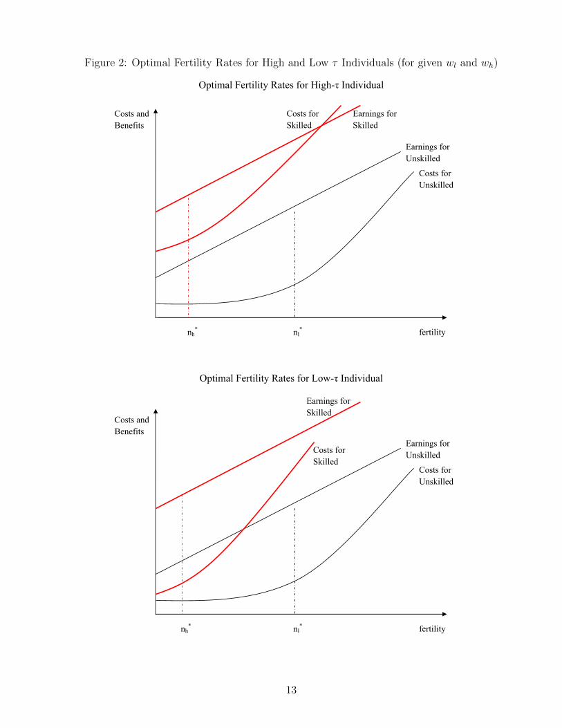
Figure 2: Optimal Fertility Rates for High and Low τ Individuals (for given wl and wh)

Optimal Fertility Rates for High-τ Individual

Optimal Fertility Rates for Low-τ Individual

fertility nl

*nh*

Costs for Unskilled

Earnings for Unskilled

Costs and Benefits

Earnings for Skilled

Costs for Skilled

fertility nl*nh

*

Costs for Unskilled

Earnings for Unskilled

Costs and Benefits

Earnings for Skilled

Costs for Skilled

13

was characterized more by developing economies adopting technologies from the world knowledge

frontier — a strategy that in many developing regions began only in the mid-20th century (Pack

and Westphal 1986, Romer 1992).

The simulations demonstrate a number of things. Early industrialization in both regions was

unskilled labor intensive (O’Rourke et al. 2013). Trade between the two regions generates some

income convergence early on — specialization induces the North to devote R&D resources to

the skill-intensive sector and the South to devote resources to the unskilled-intensive sector.

Because the skilled sector is so much smaller than the unskilled sector, the South is able to grow

relatively faster at first. But the dynamic effects of these growth paths (through fertility and

education changes) ultimately reverses income convergence. The reinforcing interactions between

technological growth and intercontinental commerce help produce dramatic divergence between

the incomes of northern and southern economies.

However, when industrialization is characterized by diffusion of technologies from the world

knowledge frontier (generated by the North) to the South, the story of income differences takes a

dramatic turn. This case produces some divergence early on due to the technology-skill mismatch

faced by the South (Basu and Weil 1998), but the North goes on to develop dramatically advanced

skill-biased technologies that are eventually implemented by the South. The South then proceeds

through its own demographic transition and catches up to the North.

Distinct from Galor and Mountford (2008), we also find that the timing of trade can affect the

relative strength of convergence or divergence. Simulations reveal how trade and technologies

feed off each other to generate growth paths that broadly mirror historic trends. We provide a

summary of our findings in the table below:

Localized Technologies Diffusion of Technologies

Early Trade Convergence then Divergence Divergence then Convergence

Delayed Trade Stronger Convergence Weaker Divergence then Weaker Convergence

We will demonstrate the impact of technological diffusion and non-diffusion in the case of

early trade growth (the cases where trade growth is delayed are demonstrated in Appendix C).

To do so however, we first need to endogenize the time paths of technologies and trade volumes.

5.1 A Dynamic Model - The Evolution of Technology and Trade

How do technologies evolve in each region? A region will either develop its own blueprints N ,

or adopt blueprints from the world frontier. The following discussion relates to the former case.

Recall that equations (18) - (20) describe one-period revenues for innovation. There must

also be some resource costs to research. We assume that these costs are rising in N (“applied”

14

knowledge, specific to each sector and to each country), and falling in some measure of “general”

knowledge, given by B (basic knowledge, common across all sectors and countries). Thus, a

no-arbitrage (free entry) condition for potential researchers in each region can be described as:

πi ≤ c

(Ni

B

)(33)

Specifically, we can assume the following functional form for these research costs:

c

(Ni

B

)=

(Ni,t+1

Bt

)ν(34)

for i = 1, 3 (for convenience we assume no research occurs in sector 2, so that technological growth

is unambiguously factor-biased. Because sector 2 is factor-neutral, relaxing this assumption does

not change any of our findings), and ν > 0. Given some level of basic knowledge (which we

can assume grows at some exogenous rate) and number of existing machines, we can determine

the resource costs of research. When basic knowledge is low relative to the number of available

machine-types used in sector i, the costs of inventing a new machine in sector i is high (see

O’Rourke et al. 2013 for a fuller discussion). Thus from (33) and (18) - (20) we see that

innovation in sector i becomes more attractive when basic knowledge is large, when the number

of machine-types in sector i is low, when then price of good i is high, and when employment in

sector i is high.

Note that if πi > c(Ni/B), there are potential profits from research in sector i. However, this

will induce research activity, increasing the number of new machines, and hence costs of research.

We assume in fact that Ni adjusts upward such that costs of research just offset the revenues

of new machine production. Thus increases in B are matched by increases in levels of Ni such

that the no-arbitrage condition holds with equality whenever technological growth in the sector

occurs.

We must also specify how trade technologies evolve. Here we use an amended version of (1),

where production for each region is given by

Y n =(α

2(yn1 + aZ1)

σ−1σ + (1− α) (yn2 )

σ−1σ +

α

2(yn3 − Z3)

σ−1σ

) σσ−1

(35)

Y s =(α

2(ys1 − Z1)

σ−1σ + (1− α) (ys2)

σ−1σ +

α

2(ys3 + aZ3)

σ−1σ

) σσ−1

(36)

Z1 is the amount of good 1 that is exported by the South, Z3 is the amount of good 3 that is

exported by the North, and 0 < a < 1 is an iceberg factor for traded goods (i.e. the proportion

of exports not lost in transit). Thus the North imports only fraction a of southern exports, and

15

the South imports only fraction a of northern exports.10 Intermediate goods production is still

described by (2) - (4). To capture improvements in transport technologies over the course of the

18th to 20th centuries, we simply have a grow exogenously each time period, such that it reaches

the limiting value of 1 by the end of the simulation.

Note that we assume that there is no trade in y2 - because this is produced using both L and

H, differences in p2 are very small between the North and the South, and thus the assumption

is not very restrictive or important.11 12

5.2 Evolution of the World Economy

General equilibrium is a thirty-six equation system that, given changes in the number of

machine blueprints and the iceberg costs, solves for prices, wages, fertility, education, labor-

types, intermediate goods, employment, trade, and sectoral productivity levels for both the

North and the South. We impose only one parameter difference between the two regions - bn <

bs (this means that there is a bigger range of resource costs for education in the South, so that the

South begins with relatively more unskilled labor than skilled labor). All other parameters are

the same in both regions. This also ensures that initial fertility and education rates, determined

endogenously here, will be different in each region. The equilibrium is described in more detail

in the appendix.

Because the model contains so many moving parts, we can only solve for general equilibrium

numerically. Specifically, we assume that both basic technology (B in eq 34) and trade technology

(a in eqs 35 and 36) start low enough so that neither technological progress nor trade are possible.

We allow however for exogenous growth in basic knowledge and trade technologies, and solve

for the endogenous variables each period. Let us first summarize the evolution of these two

economies with a few propositions, starting with the nature of early industrialization in the

world.

Proposition 1 If N1 = N3, L > H, and σ > 1, initial technological growth will be unskilled-labor

biased.

10The case where the North specializes in and exports the unskilled -intensive good and the South specializes

in and exports the skilled -intensive good is ruled out due to the North’s relative abundance of skilled labor. The

North would have to have very high levels of unskilled-biased technology compared to the South to reverse its

comparative advantage in skill-intensive production.11Indeed, trade in all three goods would produce an analytical problem. It is well known among trade economists

that when there are more traded goods than factors of production, country-specific production levels, and hence

trade volumes, are indeterminate. See Melvin (1968) for a thorough discussion.12One can conceive of y2 as the technologically-stagnant and non-tradeable “service” sector. Thus each labor-

type can work either in manufacturing or in services.

16

From (18)-(20) we can see that revenues from innovation rise both in the price of the intermediate

good (the “price effect”) and in the scale of sectoral employment (the “market-size effect). If

intermediate goods are grossly substitutable, market-size effects will outweigh price effects (see

Acemoglu 2002 for more discussion of this).

Thus as basic knowledge exogenously grows, sector 1 will be the first to modernize. The

logical implication of this is that early industrialization around the world (provided there are

intellectual property rights in these countries) will be unskilled labor intensive (O’Rourke et al.

2008).

Proposition 2 If(pn3ps3

)·(ps1pn1

)> a2, Z1 = Z3 = 0.

If transport costs are large (that is, if a is small) relative to cross-country price differences, no

trade occurs. As mentioned above, we will assume that early on transport technologies are not

advanced enough to permit trade. That is, with a small value of a, each country can produce

more under autarky than by trading. Once a reaches this threshold level, trade becomes possible,

and further increases in a allow Z1 and Z3 to rise as well.

Proposition 3 For certain ranges of factors and technologies, the trade equilibrium implies that

ys3 = 0. For other ranges of technologies and factors, the trade equilibrium implies that yn1 = 0.

As trade technologies improve, economies specialize more and more. And divergent technological

growth paths can help reinforce this specialization. There is indeed a point where the North no

longer needs to produce any y1 (they just import it from the South), and the South no longer

needs to produce any y3 (they just import it from the North). This case we will call “specialized

trade equilibrium” (described in more detail in the Appendix).

Both trade and technological changes will change factor payments. The final proposition

states how these changes can affect the factors of production themselves.

Proposition 4 If φ > 1, any increase in wl (keeping wh constant) will induce a decrease in e

and an increase in n; furthermore, so long as φ is “big enough,” any increase in wh (keeping wl

constant) will induce an increase in e and a decrease in n.

Proof.

Substituting our expressions for n∗l and n∗

h, given by (26) and (27), into our expression for τ ∗,

given by (28), and rearranging terms a bit, we get the following expression:

τ ∗ = (wh − wl) − wlλ1

1−φ

(φ

11−φ − φ

φ1−φ

)+ wl

φφ−1wh

11−φλ

11−φ

(φ

11−φ − φ

φ1−φ

)First we must have the condition ∂τ∗

∂wl< 0 hold. Solving for this and rearranging yields

17

(wlwh

) 1φ−1

< 1 +1

λ1

1−φ

(φ

11−φ − φ

φ1−φ

)Since the inverse of the skill-premium is always less than one, this expression always holds for

any φ > 1. Next we show what condition must hold in order to have the expression ∂τ∗

∂wh> 0 be

true. Solving and rearranging gives us

λ1φφ >

wlwh

Thus for a given value of λ, φ needs to be large enough for this condition to hold. Finally, our

expression for total fertility, (31), can be slightly rearranged as

n = n∗l + (n∗

h − n∗l )

(τ ∗

b

)From (26) and (27) we know that the second term is always negative, and that n∗

l is constant.

So any increase in education from wage changes will lower aggregate fertility, and any decrease

in education from wage changes will increase aggregate fertility.

5.3 Simulations13

Here we simulate the model described above to analyze the potential sources of North-South

divergence in history. Basic knowledge B and trade technology a are set such that neither

technological growth nor trade is possible at first; each however exogenously rises over time. We

run the simulation for 70 time periods to roughly capture major economic trends during two

distinct economic epochs.

5.3.1 The Case of Localized Technological Progress

Figures 3 through 5 summarize the evolution of technologies in both regions. In the beginning

the costs of research are prohibitively high everywhere, so technologies are stagnant. But growth

in basic knowledge allows us to see the implications of Proposition 1 - because there is a greater

13The parameter values used in the simulations are as follows: σ = 3, α = 0.5, γ = 0.5, λ = 0.5, φ = 10, ν = 2.

These values ensure that Propositions 1 and 4 hold - beyond that, our qualitative findings are not sensitive to

specific parameter values. We also set bn = 2, bs = 6, and pop = 2; this gives us initial factor endowments of

Ln = 3.14, Ls = 3.48, Hn = 0.86, Hs = 0.52. Initial machine blueprints for both countries are set to be N1 = 10,

N2 = 15, N3 = 10; initial trade technology is set to be a = 0.8 (here when one-fifth of trade volume is lost in

transit, each region is better off in autarky), and grows linearly such that a = 1 70 periods later; initial B is set

high enough so that growth in at least one sector is possible early in the simulation; B grows 2 percent each time

period.

18

Figure 3: Market for Technologies in North — Localized Technologies

10 20 30 40 50 60 70

Market for Northern Unskilled-Bias Technologies

valuecost

10 20 30 40 50 60 70

Market for Northern Skilled-Bias Technologies (log scale)

valuecost

19

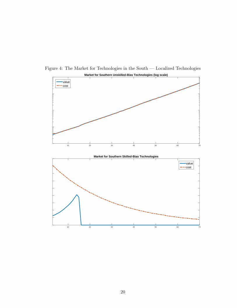
Figure 4: The Market for Technologies in the South — Localized Technologies

10 20 30 40 50 60 70

Market for Southern Unskilled-Bias Technologies (log scale)

valuecost

10 20 30 40 50 60 70

Market for Southern Skilled-Bias Technologies

valuecost

20

Figure 5: Factor Productivities — Localized Technologies

10 20 30 40 50 60 700

20

40

60

80

100

120

140Total Factor Productivities in North

A1A2A3

10 20 30 40 50 60 700

10

20

30

40

50

60

70

80

90Total Factor Productivities in the South

A1A2A3

21

abundance of unskilled labor relative to skilled labor in both the North and the South, the costs

of research first catch up to revenues in sector 1 in both regions.

This growth in unskilled labor intensive technologies increases the relative returns to unskilled

labor in both regions, inciting fertility increases and educational decreases (Proposition 4). We

can see this manifest itself in the North by the increasing revenues generated by innovation - as

population rises in the North, the market-size effects caused by fertility increases raise the value

of such innovation. Still, because skilled labor remains in relatively scarce supply, the cost of

innovation exceeds the benefits in sector 3 at the beginning of the simulation.

However the North soon starts developing skill-biased technologies as well (at t = 12). Notice

however that the South never gets to develop skill-biased technologies — looking at the lower

panel of Figure 4, something clearly happens to make the value of innovating in the sector fall

to zero.

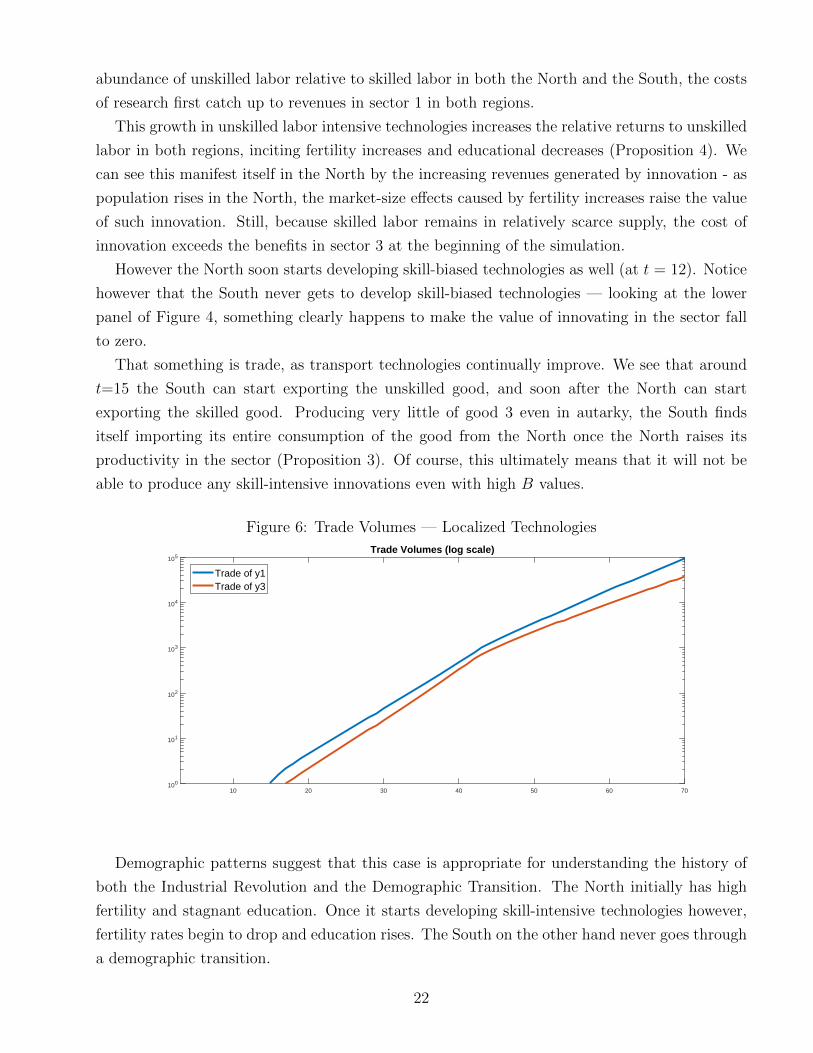
That something is trade, as transport technologies continually improve. We see that around

t=15 the South can start exporting the unskilled good, and soon after the North can start

exporting the skilled good. Producing very little of good 3 even in autarky, the South finds

itself importing its entire consumption of the good from the North once the North raises its

productivity in the sector (Proposition 3). Of course, this ultimately means that it will not be

able to produce any skill-intensive innovations even with high B values.

Figure 6: Trade Volumes — Localized Technologies

10 20 30 40 50 60 70100

101

102

103

104

105Trade Volumes (log scale)

Trade of y1Trade of y3

Demographic patterns suggest that this case is appropriate for understanding the history of

both the Industrial Revolution and the Demographic Transition. The North initially has high

fertility and stagnant education. Once it starts developing skill-intensive technologies however,

fertility rates begin to drop and education rises. The South on the other hand never goes through

a demographic transition.

22

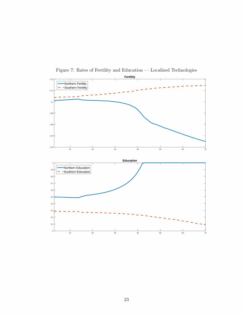
Figure 7: Rates of Fertility and Education — Localized Technologies

10 20 30 40 50 60 701.02

1.04

1.06

1.08

1.1

1.12

1.14Fertility

Northern FertilitySouthern Fertility

10 20 30 40 50 60 700

0.1

0.2

0.3

0.4

0.5

0.6

0.7

0.8

0.9

1Education

Northern EducationSouthern Education

23

To help us better understand the forces of convergence or divergence, we can decompose the

income per capita gap between the North and South into two components. Define Yn,aut as the

GDP for the North in a given year, allowing it to have the technologies from the previous, regular

equilibrium, but pretending that the North does not trade with the South. GDP per capita can

be decomposed as:

yn =

(Yn,autpopn

)(YnYn,aut

)(37)

So relative per capita incomes can be written as:

ynys

=

(Yn,autpopn

/Ys,autpops

)(YnYn,aut

/YsYs,aut

)(38)

Let us call the first term the “autarkic income per capita gap.” Let us call the second term

the “gains from trade gap.”

At first, we have convergence. Both countries have lots of unskilled workers and not as many

skilled workers, and the South gains in relative terms by developing technologies for this abundant

workforce. Indeed, we see the autarky income gap fall throughout. However, as trade continues

to grow the South loses in relative terms. Its gains from trade deteriorate because its terms of

trade deteriorate — the South must sell more and more of its unskilled good (y1) in exchange

for its imports of the skilled good (y3) (we see in Figure 6 a dramatic widening of trade volumes

between the two regions over time).

The reason has to do with relative size. The North is small and prosperous; the South is

innovative but enormous (its population grows to become ten times that of the North), flooding

the world with its product. Thus we observe economic divergence that arises from a different

source than in Galor and Mountford, but that that nevertheless has to do with interactions

between trade and technological growth.

Divergence here comes about because each region leaves its “cone of diversification.” A purely

specialized world develops, and the South specializes in that good which generates population

growth and deteriorating gains from trade with the North. Technological growth will not save

it!

What if trade was delayed? This case, displayed in Appendix C, demonstrates that the period

of convergence would be extended. The specialization patterns that immiserate Southern growth

are weakened here — each region is diversified enough to avoid the large gains from trade gap

we observe in the case described above. Contrary to Galor and Mountford (2008), we suggest

that the timing of trade liberalization can affect the pattern of per capita income divergence.

24

Figure 8: Relative Income and Divergence — Localized Technologies

10 20 30 40 50 60 700.9

1

1.1

1.2

1.3

1.4

1.5

1.6

1.7Relative Income (yn/ys)

10 20 30 40 50 60 700.5

1

1.5

2

2.5

3

3.5Decomposed Income Gap

autarky income per capita gapgains from trade gap

25

5.3.2 The Case of Perfect Technology Spillovers

Here only the North develops technologies (machine blueprints), and these flow immediately

to the South for potential use. The South in this case does not bother with research on its own

— it “allows” the North to do the research for them.

Figure 9: Market for Technologies in North — Perfect Technological Diffusion

10 20 30 40 50 60 70

Market for Northern Unskilled-Bias Technologies (log scale)

valuecost

10 20 30 40 50 60 70

Market for Northern Skilled-Bias Technologies (log scale)

valuecost

In this case we see the North innovating in both unskilled and skilled technologies early

on. However, trade forces the South to abandon skill-intensive production. Therefore even

though technologies diffuse costlessly from the North to the South, the South cannot use skilled

technologies (see Figure 10). Thus we see per capita income divergence early on — here the

channel is though “inappropriate” technological diffusion from North to South. The South is in

effect trading population for productivity (Galor and Mountford 2008), as it devotes more people

to the relatively less productive sector. Trade is modest but growing (Figure 12).

26

Figure 10: Factor Productivities — Perfect Technological Diffusion

10 20 30 40 50 60 700

10

20

30

40

50

60

70

80Total Factor Productivities in North

A1A2A3

10 20 30 40 50 60 700

10

20

30

40

50

60

70

80Total Factor Productivities in the South

A1A2A3

27

Figure 11: Rates of Fertility and Education — Perfect Technological Diffusion

10 20 30 40 50 60 701.096

1.098

1.1

1.102

1.104

1.106

1.108

1.11

1.112

1.114

1.116Fertility


10 20 30 40 50 60 700.2

0.3

0.4

0.5

0.6

0.7

0.8

0.9

1Education


28

Figure 12: Trade Volumes — Perfect Technological Diffusion

10 20 30 40 50 60 70100

101

102

103

104

Trade Volumes


However, over time the North’s specialization in skilled production makes it devote more

resources towards skill-intensive technologies. Eventually these technologies become so efficient

that the South is able to adopt them, even with its smaller skilled workforce. The fact that

the South can eventually reap the gains from Northern skilled innovation means it can finally

compete in skilled production globally. When this happens (t = 33), each country falls inside its

“cone of diversification.” The two regions begin to converge. Further, once the North reaches

universal education, convergence happens faster as the South keeps becoming more educated.

Eventually the South overtakes the North in per capita income terms.

In this case the South goes through its own demographic transition, but this is much delayed

(see Figure 11). We suggest that this case may better represent certain Southern economies

during the 20th century, which eventually successfully adopted skill-intensive technologies from

the global frontier.

What if trade were delayed in this case? Technological diffusion keeps the South structurally

close to the North, which keeps each region within its diversification cone. As long as each

region is diversified, no divergence occurs. What is interesting is that with more robust trade,

initial specialization occurs which fosters divergence, but this makes skill-biased technologies

grow faster, which then promotes faster convergence later on. In a world of knowledge diffusion,

trade can generate some divergence but this will be followed by more rapid convergence. In the

long run globalization is good for the South.

29

Figure 13: Relative Income and Convergence — Perfect Technological Diffusion

10 20 30 40 50 60 700.96

0.98

1

1.02

1.04

1.06

1.08

1.1

1.12


10 20 30 40 50 60 700.9

0.95

1

1.05

1.1

1.15

1.2



30

6 Conclusion

In this paper we provide some theoretical foundations for understanding global income di-

vergence and convergence over the last few centuries. Distinct from other works, we suggest

interactions between burgeoning trade and technological forces help us understand how diver-

gence occurred during the late 19th and early 20th centuries, as well as how convergence between

some regions occurred during the mid-20th century.

The work also provides some important testable implications. For example, the model implies

that stronger protectionist policies would have delayed the Demographic Transition in Western

Europe (see Bignon and Garcia-Penasola 2016 for recent evidence). It also implies protectionism

will have dramatically different effects when technological growth is global rather than local. The

theory here should help inform future empirical efforts in better understanding global income

divergence, both historically and more recently.

31

References

Acemoglu, Daron. 2002. “Directed Technical Change,” Review of Economic Studies 69: 781-809.

Acemoglu, Daron. forthcoming. “When Does Labor Scarcity Encourage Innovation?” Journal of

Political Economy.

Acemoglu, Daron, Simon Johnson, and James A. Robinson. 2001. “The Colonial Origins of Comparative

Development: An Empirical Investigation.” American Economic Review, 91(5): 1369-1401.

Acemoglu, Daron, Simon Johnson, and James A. Robinson. 2005. “The Rise of Europe: Atlantic Trade,

Institutional Change, and Economic Growth.” American Economic Review, 95(3): 546-79.

Acemoglu, Daron and Fabrizio Zilibotti. 2001. “Productivity Differences,” Quarterly Journal of Eco-

nomics 116: 563-606.

Aghion, Philippe and Peter Howitt. 1992. “A Model of Growth through Creative Destruction,” Econo-

metrica, 60: (323-351).

Basu, Susanto and David N. Weil. 1998. “Appropriate Technology and Growth,” Quarterly Journal of

Economics 113: 1025-1054.

Bekar, Clive and Richard Lipsey. 1997. “A Structuralist View of Technical Change and Economic

Growth.” Reprinted in Microeconomics, Growth and Political Economy: The Selected Essays of

Richard Lipsey Vol. One. Edward Elgar: Cheltenham, UK.

Bignon, Vincent and Cecelia Garcia-Penalosa. 2016. “Protectionism and the Education-Fertility Trade-

off in Late 19th Century France.” Aix-Marseille School of Economics working paper.

Clark, Gregory. 1987. “Why Isn’t the Whole World Developed? Lessons from the Cotton Mills.”

Journal of Economic History 47: 141–173.

Clark, Gregory. 2007. “A Review of Avner Grief’s Institutions and the Path to the Modern Economy:

Lessons from Medieval Trade.” Journal of Economic Literature, XLV: 727-743.

Clark, Gregory. 2007. A Farewell to Alms: A Brief Economic History of the World. Princeton and

Oxford: Princeton University Press.

Clark, Gregory, and Robert C. Feenstra. 2001. “Technology in the Great Divergence,” in NBER book

Globalization in Historical Perspective.

Clark, Gregory and Susan Wolcott. 2003. “One Polity, Many Countries: Economic Growth in India,

1873-2000.” in Dani Rodrik (ed.), Frontiers of Economic Growth. Princeton: Princeton University

Press

Crafts, N.F.R., and C.K. Harley. 1992. “Output Growth and the Industrial Revolution: A Restatement

of the Crafts-Harley View,” Economic History Review 45(4): 703-30.

Findlay, Ronald. 1996. “Modeling Global Interdependence: Centers, Peripheries, and Frontiers,” Amer-

ican Economic Review 86(2): 47-51.

Galor, Oded. 2005. “From Stagnation to Growth: Unified Growth Theory,” in Handbook of Economic

32

Growth, Vol. 1, part 1, edited by P. Aghion and S.N. Durlauf, pp. 171-293. Amsterdam: North

Holland.

Galor, Oded, and Andrew Mountford. 2002. “Why are one Third of People Indian and Chinese? Trade,

Industrialization and Demographic Transition,” manuscript.

Galor, Oded and Andrew Mountford. 2006. “Trade and the Great Divergence: The Family Connection,”

American Economic Review Papers and Proceedings, 96: 299-303.

Galor, Oded and Andrew Mountford. 2008. “Trade and the Great Divergence: Theory and Evi-

dence,”Review of Economic Studies, 75: 1143-1179.

Grossman, Gene M. and Elhanan Helpmann. 1991. Innovation and Growth in the Global Economy.

Cambridge, MIT Press.

Howitt, Peter. 1999. “Steady Endogenous Growth with Population and R&D Inputs Growing,” Journal

of Political Economy, 107: 715-730.

Jones, Charles I. 1995. “R&D-Based Models of Economic Growth,” Journal of Political Economics,

103: 759-784.

Melvin, James R. 1968. “Production and Trade with Two Factors and Three Goods,” American Eco-

nomic Review 58: 1249-1268.

Mitchener, Kris J., and Se Yan. 2010. “Globalization, Trade and Wages: What Does History Tell Us

about China?” NBER working paper no. 15679.

Mokyr, Joel. 1999. The British Industrial Revolution: An Economic Perspective, 2nd edition. Westview

Press: Boulder, CO.

Mokyr, Joel. 2002. The Gifts of Athena. Princeton, N.J.: Princeton University Press.

North, Douglass C., and Robert Paul Thomas. 1973. The Rise of the Western World: A New Economic

History. Cambridge: Cambridge University Press.

O’Rourke, Kevin H., Ahmed S. Rahman and Alan M. Taylor. 2013. “Luddites, the Industrial Revolution

and the Demographic Transition,” Journal of Economic Growth 18: 373–409.

O’Rourke, Kevin H., Alan M. Taylor and J. G. Williamson. 1996. “Factor Price Convergence in the

Late Nineteenth Century,” International Economic Review 37: 499-530.

O’Rourke, Kevin H. and Jeffrey G. Williamson. 1994. “Late 19th Century Anglo-American Factor

Price Convergence: Were Heckscher and Ohlin Right?” Journal of Economic History 54: 892-916.

O’Rourke, Kevin H. and Jeffrey G. Williamson. 1999. Globalization and History. Cambridge, MA.:

MIT Press.

Pack, Howard, and Lawrence Westphal. 1986. “Industrial Strategy and Technological Change: Theory

vs. Reality,” Journal of Development Economics 22: 87–126.

Pomeranz, Kenneth. 2000. The Great Divergence: China, Europe, and the Making of the Modern

World Economy. Princeton Economic History of the Western World series. Princeton and Oxford:

Princeton University Press.

33

Rahman, Ahmed S. 2013. “The Road Not Taken - What Is The ‘Appropriate’ Path to Development

When Growth Is Unbalanced,” Macroeconomic Dynamics 17(4): 747–778.

Romer, Paul M. 1986. “Increasing Returns and Long-Run Growth,” Journal of Political Economy, 94:

1002-1037.

Romer, Paul M. 1990. “Endogenous Technological Change,” Journal of Political Economy 98(5): S71-

S102.

Romer, Paul M. 1992. “Two Strategies for Economic Development: Using Ideas and Producing Ideas,”

Proceedings of the World Bank Annual Conference on Development Economics, Supplement to the

World Bank Economic Review, 63–91.

Segerstrom, Paul S., T. C. A. Anant, and Elias Dinopoulos. 1990. “A Schumpeterian Model of the

Product Life Cycle,” American Economic Review, 80: 1077-1092.

Temin, Peter. 1997. “Two Views of the British Industrial Revolution,” Journal of Economic History

57(1): 63-82.

Young, Alwyn. 1998. “Growth without Scale Effects.” Journal of Political Economy, 106: 41-63.

34

A Diversified Trade Equilibrium

With trade of goods y1 and y3 between the North and the South, productions in each region are

given by (35) and (36).

For each region c ∈ n, s, the following conditions characterize the diversified trade equilibrium.

ps1 =wslAs1

(39)

pc2 =

(1

Ac2

)(wcl )

γ (wch)1−γ (1− γ)γ−1γ−γ (40)

pn3 =wnhAn3

(41)

(1

Ac1

)yc1 +

(1

Ac2

)(wcl )

γ−1 (wch)1−γ (1− γ)γ−1γ1−γyc2 = Lc (42)

(1

Ac2

)(wcl )

γ (wch)−γ (1− γ)γγ−γyc2 +

(1

Ac3

)yc3 = Hc (43)

yn1 + a1Z1 =

( (α2

)σ(pn1 )−σ(

α2

)σ(pn1 )1−σ + (1− α)σ (pn2 )1−σ +

(α2

)σ(pn3 )1−σ

)· Y n (44)

ys1 − Z1 =

( (α2

)σ(ps1)

−σ(α2

)σ(ps1)

1−σ + (1− α)σ (ps2)1−σ +

(α2

)σ(ps3)

1−σ

)· Y s (45)

yc2 =

((1− α)σ (pc2)

−σ(α2

)σ(pc1)

1−σ + (1− α)σ (pc2)1−σ +

(α2

)σ(pc3)

1−σ

)· Y c (46)

yn3 − Z3 =

( (α2

)σ(pn3 )−σ(

α2

)σ(pn1 )1−σ + (1− α)σ (pn2 )1−σ +

(α2

)σ(pn3 )1−σ

)· Y n (47)

ys3 + a3Z3 =

( (α2

)σ(ps3)

−σ(α2

)σ(ps1)

1−σ + (1− α)σ (ps2)1−σ +

(α2

)σ(ps3)

1−σ

)· Y s (48)

An1 (An1Ln1 + a1Z1)

− 1σ =

(2(1− α)γ

α

)An2

σ−1σ (Ln − Ln1 )−γ−σ+σγ (Hn −Hn

3 )γ+σ−σγ−1 (49)

An3 (An3Hn3 − Z3)

− 1σ =

(2(1− α)(1− γ)

α

)An2

σ−1σ (Ln − Ln1 )−γ+σγ (Hn −Hn

3 )γ−σγ−1 (50)

35

As1 (As1Ls1 − Z1)

− 1σ =

(2(1− α)γ

α

)As2

σ−1σ (Ls − Ls1)

−γ−σ+σγ (Hs −Hs3)γ+σ−σγ−1 (51)

As3 (As3Hs3 + a3Z3)

− 1σ =

(2(1− α)(1− γ)

α

)As2


−γ+σγ (Hs −Hs3)γ−σγ−1 (52)

Ac1 =(N c

1,t−1 + αα

1−α(N c

1,t −N c1,t−1

))(αpc1)

α1−α (53)

Ac2 =(N c

2,t−1 + αα

1−α(N c

2,t −N c2,t−1

))(αpc2)

α1−α (54)

Ac3 =(N c

3,t−1 + αα

1−α(N c

3,t −N c3,t−1

))(αpc3)

α1−α (55)

Hc =

(τ∗

c

bc

)popc (56)

Lc =

(1− τ∗

c

bc

)popc + ncpopc (57)

nc =

(1− τ∗

c

bc

)n∗

c

l +

(τ∗

c

bc

)n∗

c

h (58)

ec =τ∗

c

bc(59)

pn1pn3

=Z3

aZ1(60)

ps1ps3

=aZ3

Z1(61)

Equations (39) - (41) are unit cost functions, (42) and (43) are full employment conditions, (44) -

(48) denote regional goods clearance conditions, (49) - (52) equate the marginal products of raw factors,

(53) - (55) describe sector-specific technologies, , (56) - (65) describe fertility, education and labor-types

for each region, and (66) and (67) describe the balance of payments for each region. Solving this system

for the unknowns pn1 , ps1, pn2 , ps2, p

n3 , ps3, y

n1 , ys1, yn2 , ys2, yn3 , ys3, wnl , wsl , w

nh , wsh, Ln1 , Ls1, H

n3 , Hs

3 , An1 ,

An2 , An3 , As1, As2, A

s3, L

n, Ls, Hn, Hs, nn, ns, en, es, Z1 and Z3 constitutes the static partial trade

equilibrium.

Population growth for each region is given simply by

popct = nct−1popct−1

36

Each region will produce all three goods so long as factors and technologies are “similar enough.”

If factors of production or technological levels sufficiently differ, the North produces only goods 2 and

3, while the South produces only goods 1 and 2. No other specialization scenario is possible for the

following reasons: first, given that both the North and South have positive levels of L and H, full

employment of resources implies that they cannot specialize completely in good 1 or good 3. Second,

specialization solely in good 2 is not possible either, since a region with a comparative advantage in

this good would also have a comparative advantage in either of the other goods. This implies that

each country must produce at least two goods. Further, in such a scenario we cannot have one region

producing goods 1 and 3: with different factor prices across regions, a region cannot have a comparative

advantage in the production of both of these goods, regardless of the technological differences between

the two regions. See Cunat and Maffezzoli (2002) for a fuller discussion.

B Specialized Trade Equilibrium

The specialized equilibrium is one where the North does not produce any good 1 and the South does

not produce any good 3. Productions in each region are then given by

Y n =(α

2(aZ1)

σ−1σ + (1− α) (yn2 )

σ−1σ +

α

2(yn3 − Z3)

σ−1σ

) σσ−1

(62)

Y s =(α

2(ys1 − Z1)

σ−1σ + (1− α) (ys2)

σ−1σ +

α

2(aZ3)

σ−1σ

) σσ−1

(63)

Once again, we do not permit any trade of good 2. For each region c ∈ n, s, the following conditions

characterize this equilibrium.

ps1 =wslAs1

(64)

pc2 =

(1

Ac2

)(wcl )

γ (wch)1−γ (1− γ)γ−1γ−γ (65)

pn3 =wnhAn3

(66)

(1

An2

)(wnl )γ−1 (wnh)1−γ (1− γ)γ−1γ1−γyn2 = Ln (67)

(1

An2

)(wnl )γ (wnh)−γ (1− γ)γγ−γyn2 +

(1

An3

)yn3 = Hn (68)

(1

As1

)ys1 +

(1

As2

)(wsl )

γ−1 (wsh)1−γ (1− γ)γ−1γ1−γys2 = Ls (69)

37

(1

As2

)(wsl )

γ (wsh)−γ (1− γ)γγ−γys2 = Hs (70)

a1Z1 =

( (α2

)σ(pn1 )−σ(

α2

)σ(pn1 )1−σ + (1− α)σ (pn2 )1−σ +

(α2

)σ(pn3 )1−σ

)· Y n (71)

ys1 − Z1 =

( (α2

)σ(ps1)

−σ(α2

)σ(ps1)

1−σ + (1− α)σ (ps2)1−σ +

(α2

)σ(ps3)

1−σ

)· Y s (72)

yc2 =

((1− α)σ (pc2)

−σ(α2

)σ(pc1)

1−σ + (1− α)σ (pc2)1−σ +

(α2

)σ(pc3)

1−σ

)· Y c (73)

yn3 − Z3 =

( (α2

)σ(pn3 )−σ(

α2

)σ(pn1 )1−σ + (1− α)σ (pn2 )1−σ +

(α2

)σ(pn3 )1−σ

)· Y n (74)

a3Z3 =

( (α2

)σ(ps3)

−σ(α2

)σ(ps1)

1−σ + (1− α)σ (ps2)1−σ +

(α2

)σ(ps3)

1−σ

)· Y s (75)

An3 (An3Hn3 − Z3)

− 1σ =

(2(1− α)(1− γ)

α

)An2

σ−1σ (Ln)−γ+σγ (Hn −Hn

3 )γ−σγ−1 (76)

As1 (As1Ls1 − Z1)

− 1σ =

(2(1− α)γ

α

)As2


−γ−σ+σγ (Hs)γ+σ−σγ−1 (77)

As1 =(N s

1,t−1 + αα

1−α(N s

1,t −N s1,t−1

))(αps1)

α1−α (78)

Ac2 =(N c

2,t−1 + αα

1−α(N c

2,t −N c2,t−1

))(αpc2)

α1−α (79)

An3 =(Nn

3,t−1 + αα

1−α(Nn

3,t −Nn3,t−1

))(αpcn)

α1−α (80)

Hc =

(τ∗

c

bc

)popc (81)

Lc =

(1− τ∗

c

bc

)popc + ncpopc (82)

nc =

(1− τ∗

c

bc

)n∗

c

l +

(τ∗

c

bc

)n∗

c

h (83)

38

ec =τ∗

c

bc(84)

pn1pn3

=Z3

aZ1(85)

ps1ps3

=aZ3

Z1(86)

C Cases with Delayed or No Trade

C.1 Localized Technological Growth

Here we demonstrate simulation results when altering initial trade costs. In Figure 14 we again

display the case of localized technological progress in each region for sake of comparison with alternate

cases (these are simply figures 3–8). Recall that due to specialization, each region abandons production

in one sector of the economy, causing a dramatic gains from trade gap between the two.

Figure 14: Localized Technological Growth — Baselinie

0 20 40 600

0.02

0.04

0.06Northern Tech (sector 1)

valuecost

0 20 40 600

0.5

1


valuecost

0 20 40 600

50

100

150Northern Productivities

A1A2A3

0 20 40 600

2

4

6Southern Tech (sector 1)

valuecost

0 20 40 60

×10-3

0

2

4


valuecost

0 20 40 600

50

100Southern Productivities

A1A2A3

0 20 40 601

1.05

1.1

1.15Fertility


0 20 40 600

0.5

1Education


0 20 40 60

×104

0

5

10Trade Volumes


0 20 40 600.5

1

1.5

2Relative Income (yn/ys)

0 20 40 600

2

4Decomposed Income Gap


In Figure 15 we show the same case but where trade is delayed. Here we lower initial trade technology

(a is initially set to 0.7 instead of 0.8) and then linearly raise this until it reaches one in the final period.

Here we notice a number of similarities to the prior case — the North goes through a demographic

transition while the South does not. But per capita income divergence never occurs. The reason is

that the North remains in its cone of diversification — it continues to produce y1 and thereby never

generates the kind of trade immiseration we observed earlier. Gains from trade are more balanced

39

Figure 15: Localized Technological Growth — Delayed Trade

0 20 40 600

0.5

1Northern Tech (sector 1)

valuecost

0 20 40 600

1


valuecost

0 20 40 600

50


A1A2A3

0 20 40 600

2

4


valuecost

0 20 40 60

×10-3

0

2

4


valuecost

0 20 40 600

50


A1A2A3

0 20 40 601.05

1.1

1.15Fertility


0 20 40 600

0.5

1Education


0 20 40 60

×104

0

5

10

15Trade Volumes


0 20 40 600.95

1

1.05


0 20 40 600.8

1

1.2



Figure 16: Localized Technological Growth — No Trade

0 20 40 600

1

2


valuecost

0 20 40 600

1

2


valuecost

0 20 40 600

50


A1A2A3

0 20 40 600

1

2


valuecost

0 20 40 600

1

2


valuecost

0 20 40 600

50


A1A2A3

0 20 40 601.1

1.11

1.12

1.13Fertility


0 20 40 600

0.5

1Education


0 20 40 60-1

0

1Trade Volumes


0 20 40 600.95

1

1.05


0 20 40 601

1.1

1.2



40

for each region. Thus distinct from Galor and Mountford (2008), we observe that the timing of trade

liberalization affects the nature and extent of income divergence.

In Figure 16 we show the case where trade costs are set so high that trade never occurs. Here we

have income per capita convergence. Neither region goes through a demographic transition, and each

region produces all three goods. The initial higher fertility in the South disproportionately benefits the

South as initial technologies are unskilled-bias and this advantage persists.

C.2 Perfect Technological Diffusion

Here we show similar cases of delayed or no trade, but when technologies diffuse immediately from

the North to the South. The baseline case is shown in Figure 17 (replicating figures 9–13). Recall that

here divergence occurs initially as the South abandons skill-intensive production, but that this reverses

as it can eventually adopt Northern skilled technologies.

Figure 17: Perfect Technology Spillovers — Baselinie

0 10 20 30 40 50 60 700

0.5

1


valuecost

0 10 20 30 40 50 60 700

0.5

1


valuecost

0 10 20 30 40 50 60 700

50


A1A2A3

0 10 20 30 40 50 60 700

50


A1A2A3

0 10 20 30 40 50 60 701.09

1.1

1.11

1.12Fertility


0 10 20 30 40 50 60 700

0.5

1Education


0 10 20 30 40 50 60 70

×104

0

1

2

3Trade Volumes


0 10 20 30 40 50 60 700.9

1

1.1


0 10 20 30 40 50 60 700.8

1

1.2



Figure 18 shows the same case when trade is delayed (again, initial a is set to 0.7). Here per

capita income convergence occurs throughout. The North does not develop as much skilled-intensive

technologies for the South to adopt (since Northern specialization in this sector is limited), but it also

develops more unskilled technologies that help the South. In Figure 19 where there is no trade at all,

we see that Northern technology is highly skewed towards unskilled technologies, benefiting the South

and generating income convergence throughout.

These results suggest a dynamic tradeoff for the South. Early trade here can produce divergence due

to inappropriate technology diffusion, but this gives rise to Northern technological developments that

the South will eventually be able to exploit.

41

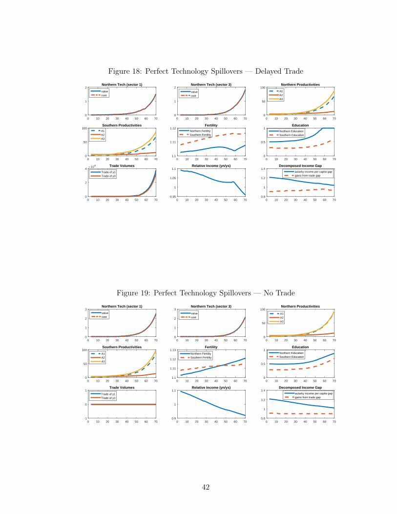
Figure 18: Perfect Technology Spillovers — Delayed Trade

0 10 20 30 40 50 60 700

1


valuecost

0 10 20 30 40 50 60 700

1


valuecost

0 10 20 30 40 50 60 700

50


A1A2A3

0 10 20 30 40 50 60 700

50


A1A2A3

0 10 20 30 40 50 60 701.1

1.11

1.12Fertility


0 10 20 30 40 50 60 700

0.5

1Education


0 10 20 30 40 50 60 70

×104

0

2

4Trade Volumes


0 10 20 30 40 50 60 700.95

1

1.05


0 10 20 30 40 50 60 700.8

1

1.2



Figure 19: Perfect Technology Spillovers — No Trade

0 10 20 30 40 50 60 700

1

2


valuecost

0 10 20 30 40 50 60 700

1

2


valuecost

0 10 20 30 40 50 60 700

50


A1A2A3

0 10 20 30 40 50 60 700

50


A1A2A3

0 10 20 30 40 50 60 701.1

1.11

1.12

1.13Fertility


0 10 20 30 40 50 60 700

0.5

1Education


0 10 20 30 40 50 60 70-1

0

1Trade Volumes


0 10 20 30 40 50 60 700.9

1


0 10 20 30 40 50 60 700.8

1

1.2



42

Trade, Technology and the Great Divergence

Documents

Transcript of Trade, Technology and the Great Divergence