Global Value Chains and Trade Policy∗

Emily J. Blanchard† Chad P. Bown‡ Robert C. Johnson§

March 29, 2021

Abstract

How do global value chain (GVC) linkages modify countries’ incentives to imposeimport protection? Are these linkages empirically important determinants of tradepolicy in practice? To address these questions, we develop a new approach to mod-eling tariff setting with GVCs, in which optimal policy depends on the nationality ofvalue-added content embedded in home and foreign final goods. Theory predicts thatdiscretionary tariffs will be decreasing in the domestic content of foreign-produced finalgoods and the foreign content of domestically-produced final goods. Using theory as aguide, we estimate the influence of GVC linkages on trade policy with data on bilat-eral applied tariffs, temporary trade barriers, and value-added contents for 14 majoreconomies between 1995 and 2015. Our empirical findings indicate that GVCs alreadyplay an important role in shaping trade policy. Governments set lower tariffs andcurb their use of temporary trade protection (particularly against China) where GVClinkages are strongest.

JEL Codes: F1, F13, F68

∗We thank Adam Szeidl and three anonymous referees, whose insights and suggestions greatly improvedthe paper. We are also grateful to Thibault Fally, Nuno Limao, Ralph Ossa, Fernando Parro, Nina Pavcnik,Raymond Robertson, and Robert Staiger for detailed feedback on early drafts. Bown acknowledges financialsupport from the World Bank’s Multi-Donor Trust Fund for Trade and Development. Carys Golesworthyprovided outstanding research assistance.

†Tuck School of Business at Dartmouth College and CEPR; emily.blanchard@tuck.dartmouth.edu‡Peterson Institute for International Economics and CEPR; cbown@piie.com§University of Notre Dame and NBER; rjohns24@nd.edu

1 Introduction

The rise of global value chains (GVCs) has transformed the nature of production. In the

modern global economy, most final goods are made by combining foreign and domestic inputs

via supply networks that traverse country borders and the traditional boundaries of the firm.

This GVC revolution has attracted widespread interest among both business leaders and

policy makers. The World Trade Organization is exploring how trade policy institutions can

be modernized to suit this new reality. Value chain concerns have also been prominent in

recent debates about the United Kingdom’s exit from the European Union and the re-design

of the North American Free Trade Agreement.1 This policy emphasis derives from a tacit

expectation that GVC linkages alter the conventional calculus of trade protection; that by

knitting together the interests of firms and workers across national boundaries, GVCs are

reshaping the consequences of tariffs and other border barriers, and hence the objectives of

government policy.

Despite the attention afforded to GVCs by practitioners, they are largely absent in ex-

isting theoretical and empirical analyses of trade policy. One reason is that GVCs are

a relatively new phenomenon, so data sources and methods to measure GVC linkages have

only recently been developed. A second reason is that GVCs take many different forms: some

are sequential in nature, others are are not; some are organized within firms, others at arms

length; some feature bilateral bargaining over prices, others allow for market-determined

prices; some are primarily bilateral, others involve many countries; and so on. This variety

in the structure of GVCs frustrates policy analysis, since these important modeling details

make it difficult to obtain general lessons or predictions for policy.

In this paper, we develop a new approach that leverages a value-added view of the

production process to advance both the theory and empirics of trade policy with GVCs.

We build on the idea that final goods are “made in the world” by combining domestic and

foreign primary factors via GVCs. Thus, GVCs are ultimately vehicles for trade in factor

services.2 This factor trade severs the link between the location where goods are produced

and the nationality of who earns the income generated from that production. Developing

this insight, we show that government objectives over final goods tariffs can be characterized

1For the WTO, see the Made in the World Initiative and the 2014 World Trade Report [WTO (2014)].See also Baldwin (2012) and Hoekman (2014). See Financial Times (2017) for discussion of supply chainconsequences of Brexit, and Blanchard (2017) on NAFTA. Lobbying materials by the TPP Apparel Coalitionon the (now defunct) Trans-Pacific Partnership and a high profile dispute between Nike and New Balanceconcerning United States import tariffs [Wall Street Journal (2013)] are testimony to the role of value chainconcerns in shaping corporate positions on trade policy.

2Our approach is conceptually related to task trade approach of Grossman and Rossi-Hansberg (2008),in that we abstract from trade in physical inputs at intermediate stages of processing. Adao, Costinot andDonaldson (2017) also advocate for models of factor exchange.

1

in terms of two basic GVC features: the pattern of trade in factor services, which defines

how income generated by final goods production is apportioned across countries, and the

system of pass-through elasticities that govern how income paid to agents engaged in the

GVC depends on final goods prices. This approach reduces a complex trade policy problem

to a tractable, intuitive one. Further, because GVC income is tied to the value-added content

of final goods, we are able to capitalize on recent advances in measuring value-added contents

to connect theory with trade policy empirics.

Embedding this production structure into a workhorse model of trade policy, we show that

final goods tariffs will be decreasing in both the amount of domestic GVC income generated

by production of foreign final goods and the amount of foreign GVC income generated by

production of domestic final goods. We then assemble rich new data on bilateral applied

tariffs, temporary trade barriers (TTBs), and value-added contents to estimate the influence

of GVC linkages on trade policy outcomes for 14 major economies over the 1995-2015 period.

Our empirical findings support the key mechanisms underlying the theory; global value chains

are already reshaping the contours of trade policy.

Our framework and results contribute to the trade policy literature in several ways.

The first contribution is to extend the canonical theory of trade policy to include GVC

linkages. To highlight the essential mechanics, we note that the use of GVC inputs in

production drives a wedge between national income and the value of final goods produced

in each country: some revenue from domestic final goods production ultimately accrues to

foreigners via GVC linkages, while some foreign final goods revenue is paid to home residents.

This re-conceptualization of the production process changes the mapping from prices to

income, and hence welfare, relative to standard models. Further, it captures the most crucial

aspects of GVCs, while remaining deliberately agnostic about non-essential micro-economic

details.3 This flexibility offers two important advantages: first, it implies that the mechanism

we emphasize is implicitly embedded in all existing models of GVCs; second, it allows us

to investigate the influence of GVCs empirically without imposing stringent, difficult-to-

quantify microeconomic assumptions.

We develop the theory in several steps. We first present the main argument in a bench-

mark two-good, two-country model with specific factors. We characterize the equilibrium

relationship between GVC linkages and optimal tariffs on final goods, and we derive the com-

3While our value-added (factor exchange) approach distills the government’s tariff problem for final goods,it is not appropriate for studying optimal input tariffs. We discuss this distinction in Section 2.5. From anempirical perspective, our focus on final goods tariffs turns into a benefit. Multilateral input tariffs are low,both in absolute terms and relative to final goods tariffs [Bown and Crowley (2016)]. We therefore focus ourtheory of how GVCs influence discretionary policy on instruments (final goods tariffs) that governments usemost often in practice.

2

parative statics that underlie our empirical approach. In a pair of extensions, we demonstrate

that the key results are robust to allowing for endogenous reorganization of GVCs in response

to tariffs, and we address the role of input tariffs, providing the theoretical basis for our focus

on how GVCs modify protectionist motives over final goods.

The theory predicts that final goods tariffs deviate from the standard “inverse export

supply elasticity rule” for two reasons. First, when foreign producers use inputs from the

home country in production, the importing country’s incentive to manipulate the terms of

trade is diminished.4 Put simply, an importer’s tariff pushes down the price that foreign

producers receive for their output, which hurts upstream domestic interests that supply

inputs to that foreign industry. Thus, all else equal, a country will set lower tariffs against

imports that embody more of its own domestic value-added content. Second, when domestic

producers use foreign inputs in production, some of the protectionist rents from higher tariffs

accrue to foreign input suppliers. This effect also dampens the government’s motivation to

apply import protection.5

Preparing to take these theoretical predictions to the data, we extend the stylized two-

by-two model to allow for many countries and many goods. We also incorporate political

economy motives for government policy, in the tradition of Grossman and Helpman (1994).

In this extended model, we characterize unilaterally-optimal bilateral tariffs for final goods.

In addition to providing bilateral, industry-specific predictions, this model sheds light on how

political economy concerns interact with GVC linkages. If the government affords additional

political weight to domestic suppliers of inputs used in foreign production, then the tariff

liberalizing effect via the first channel will be stronger. Conversely, if the government affords

political weight to foreign suppliers of inputs to domestic producers, then these political

concerns may weaken (or even overturn) the second channel. In addition to these new

results, the model also features the standard result that politically-optimal tariffs rise if

the government favors domestic producers of final goods, which is an important empirical

consideration [Goldberg and Maggi (1999); Gawande and Bandyopadhyay (2000)].

We then advance this analysis further, by describing how two important institutional

features of the world trading system – the GATT most-favored-nation (MFN) rule and Article

XXIV regional trade agreements – may lead applied tariffs to deviate from the unconstrained,

unilaterally-optimal policy. Specifically, the MFN rule constrains applied bilateral tariffs to

4While our model features a terms-of-trade motive for protection, the basic insights are portable toalternative environments, including models that feature extensive margin adjustments and de-location effectsin addition to (or instead of) conventional terms-of-trade motives.

5Importantly, this second effect arises even if the government has no ability (or motive) to manipulateits terms of trade; this channel thus constitutes a distinct international externality that travels throughdomestic prices.

3

be set at or below a country’s multilateral MFN tariff. At the same time, some bilateral tariffs

are set via regional trade agreements, in which terms-of-trade concerns may be neutralized

by cooperative negotiation [Grossman and Helpman (1995b); Bagwell and Staiger (1999)].

We account for both these institutions in our empirical strategy. The result is a framework

for bilateral trade policy analysis in the presence of institutional constraints; this framework

is an ancillary contribution that can be used for a variety of empirical applications.

Building on this foundation, we combine data on bilateral import protection and value-

added content to estimate the influence of GVC linkages on tariff-setting in practice. Our

analysis focuses on dimensions of policy over which governments have scope to implement

discretionary levels of protection.6 We first examine bilateral tariff preferences – downward

deviations in applied bilateral tariffs from multilateral MFN levels. We then examine the

use of temporary trade barriers (antidumping, safeguards, and countervailing duties) in

a separate, complementary exercise. Throughout, we measure value-added contents using

input-output methods and data from the World Input-Output Database.

Theory motivates the empirical specifications we adopt and our identification strategy.

We control for confounding factors via observable control variables (e.g., the inverse import

penetration ratio) and flexible fixed effects (which absorb variation in export supply elastic-

ities). We attend to the institutional environment in which policy is set, first by accounting

for censoring due to the MFN rule, and then exploring how the role of GVC linkages dif-

fers across trade policy regimes (e.g., inside versus outside RTAs). We also explore how

economic forces shape coefficient heterogeneity in our sample, focusing the role of upstream

and downstream product differentiation in shaping the pass-through elasticities from GVC

income to optimal tariffs. We address threats to identification, which arise from potential

simultaneity and omitted variables concerns, by using instrumental variables and controlling

for observable proxies for potential confounding effects.

Our results support the theoretical predictions: higher domestic value-added content in

foreign final goods, and higher foreign value-added content in domestic goods, are associated

with systematically larger tariff preferences. Consistent with previous work on ‘Protection for

Sale’ type political economy forces, we also find that tariff preferences are smaller – protection

is greater – when the import penetration ratios is low. Further consistent with theory, the

liberalizing effect of domestic content in foreign goods holds for tariffs set outside of RTAs,

but not for those set within RTAs. The influence of domestic content is also strongest when

it originates in upstream sectors that are differentiated, indicative of a strong pass-through

6Our study is thus in the tradition of earlier work examining unconstrained dimensions of policy, includingTrefler (1993), Goldberg and Maggi (1999), Gawande and Krishna (2003), Broda, Limao and Weinstein(2008), Bown and Crowley (2013), and Blanchard and Matschke (2015), among others.

4

from final goods prices to returns to upstream factors, and in downstream final goods sectors

that are differentiated, which likely feature lower export supply elasticities. The estimated

influence of GVC linkages on tariffs becomes stronger when we instrument for value-added

content, and when we correct for censoring of applied bilateral tariffs induced by the MFN

rule.

Finally, we show that temporary trade barriers (TTBs) respond to GVC linkages in

much the same way as bilateral applied tariffs. These results both corroborate our findings

for tariffs and extend our analysis to include these increasingly important discretionary

trade policy instruments. Refining the analysis further, we find the role of domestic content

in foreign production to be strongest for TTB-use against China, where antidumping and

other TTBs were most actively deployed during the 1995-2015 period. The data suggest

that governments are most likely to curb protectionist application of TTBs where value

chain linkages are strongest, particularly when China is the target.

Our study is related to several recent contributions to the theory of trade policy. Our

framework complements work by Ornelas and Turner (2008, 2012) and Antras and Staiger

(2012), who analyze how bilateral bargaining among value chain partners alters the mapping

from tariffs to prices, and therefore optimal trade policy for both final goods and inputs. In

contrast to these approaches, we are agnostic about the nature of price determination within

global value chains, and our results over optimal final goods tariffs obtain even if prices are

determined by market clearing conditions, as in conventional models.

More recently, Antras et al. (2021) and Caliendo et al. (2021) study optimal tariffs in

quantitative models with roundabout production and imperfect competition. Beshkar and

Lashkaripour (2020) conduct related analysis of optimal policy in a quantiative Ricardian

framework with perfect competition.7 While these very recent contributions advance the

literature in a number of directions, the upshot is that optimal input tariffs depend critically

on the precise modelling assumptions one adopts (see Antras and Chor (2021) for a summary

of this nascent literature). This constrasts with our theoretical findings for final goods tariffs,

as we discuss at length in Section 2.5.

Our theory is also related to Blanchard (2007, 2010), which show that foreign direct

investment and international ownership alter the mapping from prices to income, and thus

optimal tariffs. In contrast to this work on ownership concerns, our theory links observable

input trade patterns to bilateral tariffs. In this way, it hones in on arguably the most im-

portant dimension of GVC activity – the input linkages that accompany GVCs. Because

7Beshkar and Lashkaripour (2020) offer an elegant theoretical characterization of optimal trade taxes.A subtle but critically-important feature of their analysis is that it allows for export taxes, in addition toimport tariffs. In contrast, we rule out export taxes, which are seldom used and even unconstitutional inthe United States.

5

these input linkages are both pervasive and large quantitatively – foreign value added ac-

counts for 20 percent of the value of final manufacturing output in many countries, and

more than 50 percent in some countries and sectors – the role of input linkages is fruitful yet

previously-unexplored territory for both theoretical and empirical analysis.

Our results also contribute to the empirical literature on trade policy. Our evidence

linking the domestic value-added content in foreign production to preferential tariffs and

TTBs fits into a prominent literature studying terms-of-trade motives for protection [Broda,

Limao and Weinstein (2008); Bagwell and Staiger (2011); Ludema and Mayda (2013); Bown

and Crowley (2013); Soderbery (2018); Nicita, Olarreaga and Silva (2018)]. We are the first

(to our knowledge) both to demonstrate the relevance of terms-of-trade concerns for bilateral

tariff policy, and to document that tariffs set via RTAs behave in a manner consistent with

the neutralization of terms-of-trade motives. Our empirical findings are also consistent with

recent work on the influence of multinational firms. Blanchard and Matschke (2015) show

that the United States is more likely to offer preferential market access to destinations that

host affiliates of US multinational firms, and Jensen, Quinn and Weymouth (2015) find that

US multinationals refrain from filing antidumping disputes against countries with which they

conduct substantial intrafirm trade.

Finally, a couple of very recent papers leverage the value-added approach we develop in

this paper and find results that echo our findings in different contexts. Ludema et al. (2019)

explore the structure of protection and Chinese processing trade. Adapting the theory and

bringing new data to bear, they find that input customization and political economy forces

play an important role in shaping the relationship between GVCs and trade protection.

Focusing instead on the discretionary removal of trade protections after the creation of the

WTO, Bown, Erbahar and Zanardi (2020) find that bilateral DV A linkages predict the

probability that duties will be removed, consistent with our findings.

Finally, this paper contributes to a recent literature that applies input-output methods

to measure the value-added content of trade [Johnson and Noguera (2012); Koopman, Wang

and Wei (2014); Los, Timmer and de Vries (2015)]. Drawing on this work, we examine the

implications of value-added contents for a particular set of economic policies.

The paper proceeds as follows. Section 2 presents the theory in a benchmark two-by-two

model, derives comparative statics, and explores extensions with endogenous GVC formation

and input tariffs. Section 3 bridges from theory to data, laying out our empirical strategy

for investigating applied tariffs and describing the data. Section 4 presents the main empir-

ical results for tariff preferences. Section 5 presents complementary empirical findings for

Temporary Trade Barriers. Section 6 concludes.

6

2 Theory

In this section, we describe how global value chain linkages influence tariff setting in a two-

country, two-good (2x2) environment, in the tradition of Johnson (1953-1954). To maintain

focus, we restrict attention to a single trade policy instrument: an ad-valorem tariff applied

to imports of a final good that is produced via a global value chain.

We lay out the baseline model in Section 2.1, in which we assume that the final good is

produced by combining domestic and foreign specific factors (GVC inputs). In Section 2.2,

we characterize the implicit function that links final goods tariffs to the (potentially observ-

able) domestic value-added content of foreign goods and the foreign value-added content of

domestic goods. We also provide a comparative statics proposition that traces exogenous

changes in the endowment of GVC inputs through to optimal tariffs in Section 2.3. We

then discuss two extensions of the baseline model. First, in Section 2.4, we relax the specific

factors assumptions to allow for endogenous changes in GVC inputs in response to tariffs.

Second, we describe how input tariffs can be incorporated into the theory in Section 2.5.

2.1 The 2x2 Benchmark Model

Section 2.1.1 describes the economic environment. Section 2.1.2 characterizes the economic

equilibrium as a function of the tariff.

2.1.1 Economic Environment

Two countries, indexed by c ∈ h, f and referred to as Home and Foreign, are populated

with a continuum of identical agents who produce, trade, and consume two goods, indexed

by s ∈ x, y. Let good y serve as the freely-traded numeraire, and let pc denote the local

price of good x measured in units of good y in country c. Together, the residents of each

country hold claims on all of the country’s endowments.

Preferences Agents in each country have identical Gorman form preferences, represented

by the utility function: U(dcx, dcy), where dcs denotes consumption of good s in country c.

Factor Endowments There are two types of factors. The first is a homogeneous factor

(e.g., undifferentiated labor), which is perfectly mobile across sectors, but immobile across

countries. The second is a set of specific factors, which we refer to as “GVC inputs.” For now,

assume that these GVC inputs are specific to the destination country and sector in which

they are used to produce final goods. Let νch (νcf ) denote the quantity of the Home (Foreign)

GVC input used in production of final good x in country c, and let ~νc ≡ (νch, νcf ). (Regarding

7

notation, superscripts will denote country location of final production, and subscripts identify

the origin country of the GVC input.)

Technology Goods are produced under constant returns by atomistic firms in perfectly

competitive markets. The numeraire good y is produced using homogeneous labor, while

good x is produced by combining labor with GVC inputs. Production technologies are

summarized by the following production functions:

qcx = f cx(lcx, ν

ch, ν

cf ), and qcy = lcy, (2.1)

where qcs is output of good s in country c, and lcs is the quantity of homogeneous labor used

in production of good s.

This stylized depiction of the production process captures two essential features of global

value chains. First, both domestic and foreign factors of production are used to produce

output in a GVC. Second, GVCs often feature a high degree of input specificity and lock-in

between buyers and suppliers, as emphasized by Antras and Staiger (2012). In our model,

this lock-in is manifest as factor specificity.8

Consistent with perfect competition, GVC inputs capture all residual profit (quasi-rent)

from local final good production. In this specific factors setting, this rent depends only on the

local price of good x (pc) and the quantities of GVC inputs available for use in production

(~νc). We are deliberately agnostic about the exact division of these quasi-rents between

Home and Foreign input owners; We assume only that the mapping from final goods prices

to the return to each GVC input is well-defined and positive.9 Using rch (rcf ) to denote the

per-unit return to νch (νcf ), we formalize this assumption as follows:

Assumption 2.1. rcj ≡ rcj(pc;~νc) where

∂rcj (pc;~νc)

∂pc> 0 for c, j ∈ h, f.

This assumption rules out the possibility that a change in final goods revenue could lead to

redistribution of rents between different input suppliers such that the return to one input

(weakly) declines while the return to the other rises.10

8An important feature of this setup is that the production function is written in terms of primary factorinputs. This allows us to avoid specifying various microeconomic details about how intermediate inputs aretransformed into final goods. A simple two-stage interpretation of the model is that intermediate inputsare produced at home (from domestic factors) and shipped abroad to be combined with foreign factors andassembled into final goods. More complicated value chains, in which inputs cross borders many times, arealso compatible with our reduced-form representation of the production process.

9The division of rents is indeterminate with multiple specific factors. In a more general model, thedivision of rents would depend on supply-side primitives regarding frictions that govern matching betweenGVC input suppliers and final goods producers, bargaining power of different agents, etc.

10Outside a specific factors setting, the return to value-added inputs will depend on both the Home andForeign price; we discuss this possibility further in Section 2.4.

8

Tariffs and Timing We assume that x is Home’s natural import good and allow the Home

government to impose an ad-valorem tariff on imports, applied to the Foreign selling price.11

The government chooses its tariff to maximize aggregate indirect utility of Home residents,

subject to balanced budget constraints and global market clearing conditions. Taking the

tariff as given, firms maximize profits and consumers maximize welfare. The government has

perfect foresight and there is no uncertainty in the model.

Both countries are assumed to be “large,” in that government tariff choices may affect

market-clearing prices. Following common practice [e.g. Bagwell and Staiger (1999)], we

rule out the Metzer and Lerner paradoxes to ensure that an increase in the home country’s

tariff causes the price of the imported good to rise at Home and fall abroad. Using τ to

represent one plus the tariff and pc to represent the equilibrium price of good x in country

c, we assume that:

Assumption 2.2. dpf

dτ≤ 0 ≤ dph

dτ.

2.1.2 Model Solution

Production The technology for the numeraire good y normalizes the equilibrium wage to

one in both countries. Profit maximization by atomistic firms and the local labor market

clearing condition then determine the allocation of labor across sectors according to:

lcx(pc;~νc) = arg max

lcxpcf cx(l

cx, ν

ch, ν

cf )− lcx, (2.2)

lcy(pc;~νc) = Lc − lcx(pc;~νc), (2.3)

where Lc is the total local labor endowment in country c and lcx + lcy ≤ Lc.12 Substituting

these labor allocation functions into the production functions yields the supply function for

each good:

qcx(pc;~νc) = f cx(l

cx(p

c;~νc);~νc) (2.4)

qcy(pc;~νc) = lcy(p

c;~νc). (2.5)

11Export taxes are ruled out, since they are seldom used in practice, and even unconstitutional in theUnited States. From a theoretical perspective, allowing Foreign to charge an exogenous export tax wouldintroduce an additional parameter to the model, but would not otherwise affect the predictions of the theory.

12To streamline notation, we suppress Lc as an argument going forward.

9

With perfect competition, GVC inputs capture residual profits from final good production,

denoted πcx, which depend on the local price and factor use:

πcx(pc;~νc) ≡ rch(p

c;~νc)νch + rcf (pc;~νc)νcf = pcqcx(p

c;~νc)− lcx(pc;~νc). (2.6)

Consumption With Gorman form preferences, aggregate demand and indirect utility de-

pend only on local prices and aggregate national income:

dcx(pc, Ic) = arg max

dcxU(dcx, d

cy) s.t. dcy + pcdcx ≤ Ic, (2.7)

dcy(pc, Ic) = Ic − pcdcx(pc, Ic), (2.8)

V (pc, Ic) = U(dcx(pc, Ic), dcy(p

c, Ic)), (2.9)

where V (·) is indirect utility and Ic is national income.

National Income In turn, national income is the sum of factor payments plus tariff

revenue, Rc:

Ic = Lc + rhc (ph;~νh)νhc + rfc (pf ;~νf )νfc +Rc. (2.10)

Home tariff revenue is Rh = (ph − pf )Mx(~p, Ih;~νh), where Mx(·) ≡ dhx(p

h, Ih) − qhx(ph;~νh)

is Home’s imports of good x; since Foreign practices free trade, Rf = 0. Because income

depends on tariff revenue, and tariff revenue depends on income, Equation (2.10) implicitly

defines income as a function of prices and GVC input use: Ic ≡ Ic(~p;~ν).

Equivalently, national income can be written (implicitly) as the sum of the value of

domestic final good production at local prices and tariff revenue, less payments to foreign

GVC inputs used in domestic production (FV A), plus income earned by domestic GVC

inputs used in foreign production (DV A):

Ic = pcqcx(pc;~νc) + qcy(p

c;~νc) +Rc − rcj(pc;~νc)νcj︸ ︷︷ ︸≡FV Ac

+ rjc(pj;~νj)νjc︸ ︷︷ ︸≡DV Ac

, (2.11)

where j 6= c. The first three components of this expression mirror standard models. The

last two components reflect GVC linkages. Foreshadowing results to come, note that FV Ac

and DV Ac depend on final goods prices via the endogenous return to GVC inputs. Because

tariffs influence these final goods prices, trade policy affects income in a non-standard way

in the presence of GVCs.

10

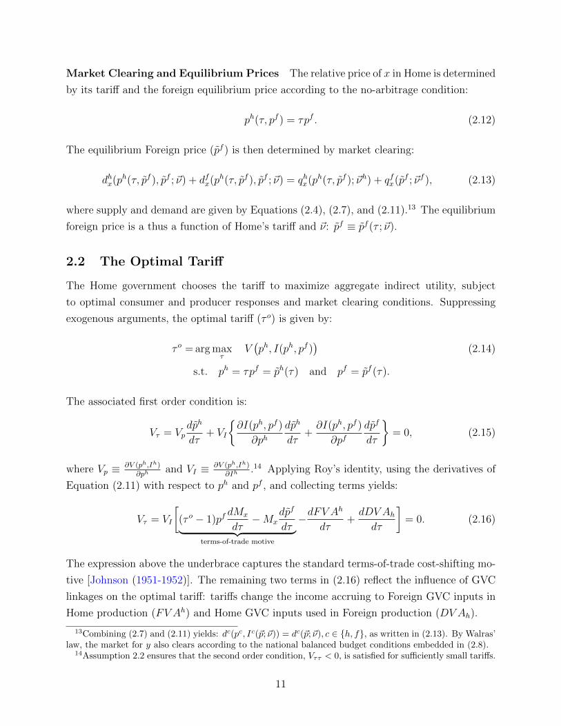
Market Clearing and Equilibrium Prices The relative price of x in Home is determined

by its tariff and the foreign equilibrium price according to the no-arbitrage condition:

ph(τ, pf ) = τpf . (2.12)

The equilibrium Foreign price (pf ) is then determined by market clearing:

dhx(ph(τ, pf ), pf ;~ν) + dfx(p

h(τ, pf ), pf ;~ν) = qhx(ph(τ, pf );~νh) + qfx(pf ;~νf ), (2.13)

where supply and demand are given by Equations (2.4), (2.7), and (2.11).13 The equilibrium

foreign price is a thus a function of Home’s tariff and ~ν: pf ≡ pf (τ ;~ν).

2.2 The Optimal Tariff

The Home government chooses the tariff to maximize aggregate indirect utility, subject

to optimal consumer and producer responses and market clearing conditions. Suppressing

exogenous arguments, the optimal tariff (τ o) is given by:

τ o = arg maxτ

V(ph, I(ph, pf )

)(2.14)

s.t. ph = τpf = ph(τ) and pf = pf (τ).

The associated first order condition is:

Vτ = Vpdph

dτ+ VI

∂I(ph, pf )

∂phdph

dτ+∂I(ph, pf )

∂pfdpf

dτ

= 0, (2.15)

where Vp ≡ ∂V (ph,Ih)∂ph

and VI ≡ ∂V (ph,Ih)∂Ih

.14 Applying Roy’s identity, using the derivatives of

Equation (2.11) with respect to ph and pf , and collecting terms yields:

Vτ = VI

[(τ o − 1)pf

dMx

dτ−Mx

dpf

dτ︸ ︷︷ ︸terms-of-trade motive

−dFV Ah

dτ+dDV Ahdτ

]= 0. (2.16)

The expression above the underbrace captures the standard terms-of-trade cost-shifting mo-

tive [Johnson (1951-1952)]. The remaining two terms in (2.16) reflect the influence of GVC

linkages on the optimal tariff: tariffs change the income accruing to Foreign GVC inputs in

Home production (FV Ah) and Home GVC inputs used in Foreign production (DV Ah).

13Combining (2.7) and (2.11) yields: dc(pc, Ic(~p;~ν)) = dc(~p;~ν), c ∈ h, f, as written in (2.13). By Walras’law, the market for y also clears according to the national balanced budget conditions embedded in (2.8).

14Assumption 2.2 ensures that the second order condition, Vττ < 0, is satisfied for sufficiently small tariffs.

11

With an eye toward empirical applications, we decompose dFV Ah

dτand dDV Ah

dτas follows:

dFV Ah

dτ=dFV Ah

dphdph

dτ=

(drhfdph

ph

rhf

)︸ ︷︷ ︸≡εrhf >0

rhfνhf

ph+

dph

dτ+

= εrhfFV Ah

phdph

dτ> 0, (2.17)

dDV Ahdτ

=dDV Ahdpf

dpf

dτ=

(drfhdpf

pf

rfh

)︸ ︷︷ ︸≡εrfh >0

rfhνfh

pf+

dpf

dτ–

= εrfhDV Ahpf

dpf

dτ< 0. (2.18)

Here εrhf and εrfh represent the elasticity of the return to GVC inputs with respect to changes

in the local final goods price in Home and Foreign, respectively. These elasticities are positive

under Assumption 2.1: an increase in the factory-gate price of a given final good implies

higher returns to all of the value-added inputs used to make it.15

Substituting Equations (2.17) and (2.18) into the first order condition, applying the

market-clearing condition, and isolating τ o, we arrive at an implicit function that defines the

optimal tariff:

τ o = 1 +1

εfx

(1− εrfh

DV Ah

pfEfx

− εrhfFV Ah

phEfx

1

|λ|

), (2.19)

where λ ≡ dpf

dτ

/dph

dτ< 0 and εfx > 0 is foreign export supply elasticity.16

This expression echoes the canonical solution for the optimal tariff of a national-income

maximizing government, as in Johnson (1951-1952), but it is modified to incorporate GVC

linkages. Specifically, the inverse export supply elasticity captures the terms-of-trade motive

for tariff setting by large countries;17 GVC linkages alter that motive in two ways.

First, the use of Home GVC inputs in foreign production serves to dampen the terms-

of-trade cost-shifting motive. The reason is that dDV Ahdτ

= dDV Ahdpf

dpf

dτ< 0: an increase in

Home’s tariff, which lowers the price of foreign-produced final goods, is passed back through

the value chain (in the form of lower returns) to Home’s suppliers of GVC inputs used in

foreign production. In effect, GVC links lead the large importing country to internalize some

of the terms-of-trade externality. As in Equation (2.18), the strength of this mechanism is

increasing with the pass-through elasticity from foreign final goods prices to domestic GVC

15Note that Home’s tariff affects GVC income only through local final goods prices. In a model withendogenous GVC inputs and sufficient input substitutability across borders and/or sectors, GVC incomedepends on the complete vector of final goods prices worldwide; see Appendix A.3.

16 In the presence of GVCs, export supply elasticity includes potential Foreign income effects from changes

in GVC income. Thus, we define: εfx ≡ εfx(τ, ~ν) = pf

Efx

dEfx(p

f ,If )dpf

+∂Ef

x(pf ,If )

∂IfdFV Adph

pf

λEfx

, where the first term

is the direct analog to the trade elasticity in conventional models without GVC income.17When foreign export supply is less elastic, the Home government has greater market power to improve

its terms of trade at the expense of foreign exporters and will therefore set a higher tariff.

12

inputs (εrfh ) and the magnitude of the GVC input trade (DV Ah).

Second, the use of Foreign GVC inputs in Home production gives rise to a second, distinct

spillover channel. An increase in Home’s tariff raises income earned by those foreign factors

of production, dFV Ah

dτ= dFV A

dphdph

dτ> 0: Home’s tariff raises the price received by domestic

import-competing final goods producers, at the expense of domestic consumers. When Home

production uses foreign-sourced GVC inputs, some of the protectionist rents generated by

this price increase are passed back upstream to Foreign input suppliers. This FV A pass-

through mechanism – from Home’s tariff to its domestic price, and from the domestic price to

the return to Foreign GVC inputs embedded in domestic production – constitutes a distinct

domestic-price externality that also serves to drive down the optimal tariff, all else equal.

The strength of the mechanism is again increasing with the pass-through elasticity εrhf and

the magnitude of GVC input trade (FV Ah).

In Equation (2.19), we further note that the trade volume (Efx ) and the elasticity of trade

(εfx) scale the (direct) relationship between the GVC terms and the optimal tariff. This is

because the trade volume influences the strength of GVC linkages as a counterweight to

the terms-of-trade motive. All else equal, higher trade volumes magnify the terms-of-trade

motive relative to the (direct) trade-liberalizing influence GVC linkages.

The optimal tariff expression in Equation (2.19) offers valuable insights into the equi-

librium relationship between the tariff level and the elasticity of trade, trade values, pass-

through elasticities, and GVC income. Further, by linking optimal tariffs to potentially-

observable GVC income linkages, it will serve to structure our empirical investigation to

follow. Before pushing forward in that direction, we pause to present comparative statics

results that describe how optimal tariffs change in response to exogenous changes in GVCs.

2.3 Comparative Statics

In this section, we characterize the impact of exogenous changes in the endowment of GVC

inputs on the optimal tariff. Specifically, consider an increase in either the quantity of Home

GVC inputs used in Foreign production (νfh), or the quantity of Foreign GVC inputs used in

Home production (νhf ). These changes will lead Home’s optimal tariff to decline, as long as

their direct effects outweigh their indirect effects. The following proposition formalizes this

statement.

Proposition 1. The optimal tariff is decreasing with GVC inputs νfh [νhf ] if and only if the

(unambiguously negative) direct first-order influence of νfh [νhf ] on the optimal tariff outweighs

any indirect second-order influence of νfh [νhf ] on the tariff via changes in trade volumes, trade

elasticity, and pass-through rates; i.e. if and only if Condition 1 [2] is satisfied.

13

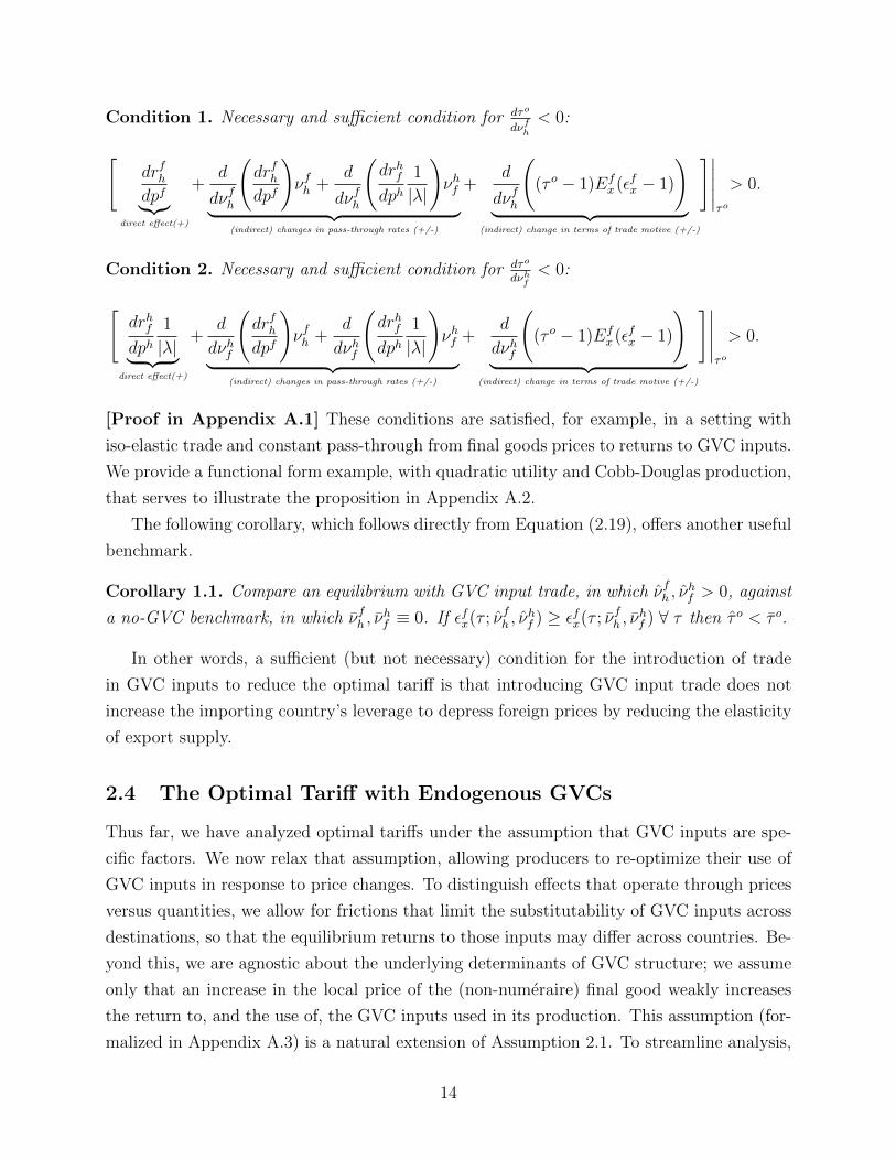
Condition 1. Necessary and sufficient condition for dτo

dνfh< 0:

[drfhdpf︸︷︷︸

direct effect(+)

+d

dνfh

(drfhdpf

)νfh +

d

dνfh

(drhfdph

1

|λ|

)νhf︸ ︷︷ ︸

(indirect) changes in pass-through rates (+/-)

+d

dνfh

((τ o − 1)Ef

x (εfx − 1)

)︸ ︷︷ ︸

(indirect) change in terms of trade motive (+/-)

]∣∣∣∣∣τo

> 0.

Condition 2. Necessary and sufficient condition for dτo

dνhf< 0:

[drhfdph

1

|λ|︸ ︷︷ ︸direct effect(+)

+d

dνhf

(drfhdpf

)νfh +

d

dνhf

(drhfdph

1

|λ|

)νhf︸ ︷︷ ︸

(indirect) changes in pass-through rates (+/-)

+d

dνhf

((τ o − 1)Ef

x (εfx − 1)

)︸ ︷︷ ︸

(indirect) change in terms of trade motive (+/-)

]∣∣∣∣∣τo

> 0.

[Proof in Appendix A.1] These conditions are satisfied, for example, in a setting with

iso-elastic trade and constant pass-through from final goods prices to returns to GVC inputs.

We provide a functional form example, with quadratic utility and Cobb-Douglas production,

that serves to illustrate the proposition in Appendix A.2.

The following corollary, which follows directly from Equation (2.19), offers another useful

benchmark.

Corollary 1.1. Compare an equilibrium with GVC input trade, in which νfh , νhf > 0, against

a no-GVC benchmark, in which νfh , νhf ≡ 0. If εfx(τ ; νfh , ν

hf ) ≥ εfx(τ ; νfh , ν

hf ) ∀ τ then τ o < τ o.

In other words, a sufficient (but not necessary) condition for the introduction of trade

in GVC inputs to reduce the optimal tariff is that introducing GVC input trade does not

increase the importing country’s leverage to depress foreign prices by reducing the elasticity

of export supply.

2.4 The Optimal Tariff with Endogenous GVCs

Thus far, we have analyzed optimal tariffs under the assumption that GVC inputs are spe-

cific factors. We now relax that assumption, allowing producers to re-optimize their use of

GVC inputs in response to price changes. To distinguish effects that operate through prices

versus quantities, we allow for frictions that limit the substitutability of GVC inputs across

destinations, so that the equilibrium returns to those inputs may differ across countries. Be-

yond this, we are agnostic about the underlying determinants of GVC structure; we assume

only that an increase in the local price of the (non-numeraire) final good weakly increases

the return to, and the use of, the GVC inputs used in its production. This assumption (for-

malized in Appendix A.3) is a natural extension of Assumption 2.1. To streamline analysis,

14

we also adopt quasi-linear preferences.

As before, Home’s national income is given by Equation (2.11), and the government

maximizes aggregate indirect utility subject to the arbitrage and market clearing conditions

described in Equation (2.14). The optimal tariff takes the form:

τ o = 1 +1

εfx

(1− (εrfh + ενfh )

DV Ah

pfEfx

− (εrhf + ενhf )FV Ah

phEfx

+ η

), (2.20)

where εfx is the foreign export supply elasticity for final goods (holding ~ν fixed), η captures

the impact of changes in final goods trade as a result of the endogenous change in input use,

and the εs are analogs to the pass-through elasticity terms in the baseline specific factors

model. See Appendix A.3 for details of the derivation and precise definition of these terms.

The first substantive difference between this expression and the corresponding optimal

tariff in the specific factors model (Equation (2.19)) is that the pass-through terms attached

to DV A and FV A now allow for potential changes in both the prices (via εr) and quantities

(via εν) of GVC inputs used in response to tariff changes. In the specific factors setting, the

εrcj terms were unambiguously positive, and the ενcj terms were identically zero. In this more

general model, the signs of εrfh + ενfh and εrhf + ενhf depend on the relative responsiveness

of GVC income to changes in local prices versus changes in prices abroad. Concretely,

εrfh + ενfh > 0 as long as the decrease in the foreign final goods price due to Home’s tariff

causes DV A to fall more than the potential increase in DV A associated with higher final

goods prices at home. Likewise, εrhf + ενhf > 0 as long as the increase in FV A induced by

the increased price of the final good at Home outweighs any potential decline in FV A due

to the decline in the foreign price of the final good. Sufficient international segmentation in

input markets will ensure that these conditions hold.18

The second difference is that there is a new term, η, in the optimal tariff, which captures

the impact of changes in GVC input use on final goods production patterns. Notably, some

or all of η may cancel with the endogenous input reallocation components of the DV A and

FV A terms (the ενs); how much depends on assumptions regarding the underlying market

structure governing input use. For example, if GVC inputs are paid the value of their

marginal product, then as frictions in input markets fall to zero, η will cancel the εν terms,

leaving just the price-pass through mechanisms (the εrs). (See Lemma 2 in Appendix A.3.)

18Ludema et al. (2019) find that when inputs are highly substitutable across end-uses and countries, andinelastically demanded by downstream producers, it is possible under certain parameter restrictions that anincrease in a home country’s tariff could cause DV A to fall. For this to happen, an increase in Home’s tariffwould need to drive up Home’s demand for the (tradeable) GVC input in Home so much that it outweighsthe negative impact of the concomitantly lower demand for the input overseas. These conditions are special,but not impossible.

15

In summary, although a more flexible production structure introduces additional adjust-

ment channels, these channels can still be summarized in terms of pass-through elasticities,

as in the specific-factors model. And although the behavior of the pass-through elasticity

terms depends on particular model assumptions, the sign of these pass-through terms will be

positive as long as the income associated with a given GVC input is more responsive to the

local price where the input is used than it is to prices elsewhere. Thus, the basic predictions

for how GVCs influence tariff setting are robust to relaxation of the specific-factors assump-

tion, as long as Home’s GVC income is decreasing in its tariffs. Accordingly, our predictions

would obtain in many models of global value chains.

2.5 Input Tariffs

In analyzing tariffs for final goods, we have abstracted from the simultaneous analysis of

input tariffs. We pause here to explain why it is both reasonable and prudent to so.

We begin by introducing input tariffs into the benchmark model. We show that an

exogenous tax on Home’s foreign-sourced GVC inputs attenuates the impact of FV A on the

optimal final goods tariff, but does not change the key directional predictions of the model.

We then consider endogenous input tariffs. In the benchmark specific factors model, we note

that endogenous input tariffs are both uninteresting and unrealistic: the optimal tariff is set

to extract all rents accruing to foreign GVC inputs. Then, we briefly discuss input tariffs in

models with endogenous GVC input use. We argue that general predictions for how input

tariffs depend on GVC linkages are elusive, in contrast to our results for final goods tariffs.

2.5.1 Input Tariffs in the Benchmark Model

Returning to the specific factors model in Section 2.1, suppose that Home levies an ex-

ogenous, ad-valorem tax g ∈ [0, 1] on the foreign-sourced GVC inputs used in domestic

production, νhf , applied to the local price of these inputs, rhf . All other assumptions and

model structure are the same.

As before, national income is given by (2.11), but tariff revenue is now:

Rh = (ph − pf )Mhx + grhfν

hf . (2.21)

Maximizing aggregate indirect utility subject to market clearing conditions, the first order

condition of Home’s optimal tariff problem is given by:

Vτ = VI

[(τ o − 1)pf

dMx

dτ−Mx

dpf

dτ− (1− g)

dFV Ah

dτ+dDV Ahdτ

]= 0. (2.22)

16

Applying the market-clearing condition, using the same tariff decompositions in Equations

(2.17) and (2.18), and isolating τ o, yields the augmented optimal tariff expression:

τ o = 1 +1

εfx

(1− εrfh

DV Ah

pfEfx

− (1− g)εrhfFV Ah

phEfx

1

|λ|

). (2.23)

The input tariff enters this optimal (final good) tariff expression in two ways. First,

the input tariff directly weakens the link between FV A and the optimal tariff: all else

equal, higher input tariffs allow the Home government to capture more of the protectionist

rents associated with final goods tariffs, dampening the tariff-liberalizing influence of FV A

on trade protection. Additionally, input tariffs may enter the optimal final goods tariff

indirectly, by changing the underlying mapping from final goods prices to input prices (and

thus the εrhf term).19 Crucially, neither of these potential effects of input tariffs on final goods

tariffs changes the directional predictions of the model. The upshot: introducing arbitrary

input tariffs does not change the basic structure of the optimal final goods tariff, or our

central finding that GVCs erode mercantilist motives for trade protection in final goods.20

2.5.2 Endogenous Input Tariffs

We now take up the question of the optimal tariff on inputs: what is the Home country’s

optimal tax (go) applied to foreign-sourced GVC inputs used in Home production? Although

the structure of this problem is similar to the optimal tariff problem for final goods, the nature

of the solution is qualitatively different. The directional relationship between input tariffs

and GVCs is fundamentally model-dependent, in a way that the relationship between final

goods tariffs and GVCs is not.

To begin, notice that allowing for an endogenous input tariff in the context of our bench-

mark specific-factors setting is trivial. If GVC inputs are fixed, the Home government would

use input tariffs to extract all rents associated with foreign-supplied inputs. The optimal

input tariff is thus a corner solution at go = 1. The associated final goods tariff would

still be given by Equation (2.23), but with g = 1, the optimal tariff would not depend on

FV A. Moreover, if the foreign government also used an optimal import tariff to extract

all of Home’s GVC income (DV A), then Home’s optimal final good tariff would collapse to

the familiar inverse elasticity rule. This makes sense: if input tariffs allow governments to

19This might be the case, for instance, if government policy disrupts bargaining outcomes between up-stream sellers and downstream buyers as in Antras and Staiger (2012).

20Adding an exogenous input tax to the model with endogenous GVC input use, described in Section 2.4,yields the general equilibrium analog to Equation (2.23). See Appendix A.4. The qualitative conclusions arethe same.

17

completely expropriate the rents associated with GVC trade, governments will behave as if

all factors of production used in local production are their own. This result, however, is as

counterfactual as it is obvious; in practice, tariffs on intermediate inputs are systematically

lower than final goods tariffs, and they are also very low in absolute terms.

Meaningful analysis of endogenous input tariffs thus requires a general equilibrium setting

in which GVC inputs respond endogenously to prices. Drawing on the framework from

Section 2.4, we analyze the optimal input tariff in Appendix A.4. For a given final good

tariff τ , the first order condition for the optimal input tariff is given by:

Vg=VI

[(τ−1)pf

dMx

dg−Mx

dpf

dg+ph∇~νqhx ·Dg~ν+

dDV Ahdg

−(1−go)dFV Ah

dg+FV A

]=0 (2.24)

On examination, it is clear that optimal input tariffs, like final goods tariffs, will be charac-

terized by an (own) inverse elasticity rule: the greater the elasticity of foreign-sourced GVC

inputs, the lower the optimal input tax on those inputs, all else equal. As is the case for

final goods tariffs, this inverse elasticity rule will be moderated by GVC linkages, reflected

in a series of cross-elasticities: how the input tariff affects the pattern of input use and thus

final goods production, prices, trade and the associated tax revenue, and DV A.

The relationship between GVCs and optimal input tariffs depends on the structure of

these cross-elasticities. Unfortunately, there is no obvious disciplining device for placing

bounds on them, which implies that one cannot easily sign the directional relationship be-

tween input tariffs and GVC linkages. Even in our simple setting, specific assumptions –

whether GVC inputs are complements or substitutes in production, or whether there are

differences in productivity across countries (so that a reallocation of inputs across countries

would change the global supply of the final good) – would be needed to pin down definitive

results.21

A signature strength of our theoretical approach to evaluating final goods tariffs is that

it side-steps hard-to-quantify production details, yet yields predictions that are amenable to

direct econometric investigation. Extending the analysis to input tariffs defeats this valuable

advantage. Thus, we set aside input tariffs for the remainder of the paper to focus on the

relationship between GVC linkages and trade protection for final goods only.

21Recent work highlights the complexity of the issue. Antras and Chor (2021) investigate the optimal tariffstructure in a stylized two-country partial equilibrium structure with a single final good, Leontief technology,and one undifferentiated input. Even with sufficient structure to sign the cross effects of input tariffs onfinal goods prices and vice versa, they find a taxonomy of outcomes and conclude that “the manner in whichvertical linkages affect optimal tariffs depends on subtle aspects of the environment.”

18

3 Theory to Data

In this section, we modify the benchmark model introduced in Section 2 to suit empirical

application, and we describe our empirical strategy and data. Section 3.1 extends the 2x2

model to allow for many sectors and countries, and introduces political economy motives for

tariff setting. In Section 3.2, we then discuss how two important institutional features of the

world trading system – the most favored nation (MFN) rule and regional trade agreements

– can be incorporated into the analysis. Section 3.3 translates the theory into an empirical

estimation framework, and Section 3.4 surveys threats to identification. We conclude by

presenting the data in Sections 3.5 and 3.6.

3.1 Many-Country, Many-Good Model with Political Economy

Building on Section 2.1, suppose the ‘home’ country (indexed by h) now produces, consumes,

and trades S final goods (in set S) plus one freely-traded homogeneous numeraire good

(indexed by 0) with C trading partners (in set C). Beyond the increase in the number of

goods and countries, there are two substantive changes in the model. We discuss them briefly

here, and refer the reader to Appendix A.5 for a complete exposition.

First, we adopt quasi-linear preferences for additional tractability, as is standard in the

literature [Grossman and Helpman (1994)]. Preferences are now given by:

U c(dh0 ,~dsh) = dh0 +

∑s∈S

us(dhs ) ∀h ∈ C, (3.1)

where ~dsh

is the vector of country h’s consumption of each non-numeraire good and sub-

utility over each non-numeraire good, us(·), is increasing, continuously differentiable, and

strictly concave. We assume that every individual has sufficient income to consume a strictly

positive quantity of the numeraire, so that demand for non-numeraire goods is independent

of income.

Second, we introduce political economy motivations for policy. Following Helpman (1997)

and Ludema and Mayda (2013), we assume that the Home government maximizes the sum of

aggregate indirect utility and a set of “special interest factors” associated with the quasi-rents

from production in different final goods sectors:

Gh = V h +∑s∈S

[δDPEs πhs + δDV As DV Ash + δFV As FV Ahs ], (3.2)

where V h is Home’s (endogenous) aggregate indirect utility, πhs is the total residual profit

19

from Home’s local production of s, DV Ash =∑

j 6=hDV Ajsh where DV Ajsh = rjsh(p

js;~ν

js)ν

jsh

is the total return to Home’s value-added inputs used in (all) foreign production of good s,

and FV Ahs =∑

j 6=h rhsj(p

hs ;~ν

hs )νhsj is the total return to (all) foreign value-added inputs used

in Home’s production of good s.

The parameters δDPEs , δFV As , and δDV As are exogenous political economy weights associ-

ated with each final goods sector s ∈ S. These weights accommodate a variety of political

economy motivations. The parameter δDPEs captures any additional consideration that the

Home government affords to rents earned in domestic final goods production of good s at

Home (πhs ). Similarly, δDV As reflects any extra political value that the Home government

places on the returns to Home’s domestic value-added inputs used in foreign final goods

production (DV Ash).22 Finally, δFV As represents the political weight (if any) given to foreign

income associated with the use of foreign value-added inputs used in Home’s production

(FV Ahs ). We do not impose a priori restrictions on these weights, but standard arguments

would imply positive values for politically active constituencies.23

Endowments, technology, and remaining model structure – including multi-country, multi-

sector analogs to Assumptions 2.1 and 2.2 – are the same as in the 2x2 benchmark model. We

allow arbitrary exogenous tariffs or other trade barriers between Home’s trading partners, but

require that prices obey a set of SC no-arbitrage conditions: phs ≤ τhscpcs,∀c 6= h ∈ C, s ∈ S,

which hold with equality when there is trade.24 Equilibrium prices are then pinned down

by a set of S market clearing conditions that ensure global demand equals global supply

for each non-numeraire good:∑

c∈C dcs(p

cs) =

∑c∈C q

cs(p

cs;~ν

cs) for all s ∈ S. Balanced budget

conditions for each country clear the market for the numeraire.

Politically-Motivated Bilateral Tariffs The Home government chooses its politically-

optimal bilateral tariffs (τhxjj 6=h) to maximize Equation (3.2), subject to balanced budget,

22Since both∑s π

hs and

∑sDV Ash are included in Home’s national income, they are already included in

V h with a weight of 1; thus, δDPEs and δDVAs capture any additional weight afforded to these rents by theHome government, above and beyond their direct contribution to aggregate welfare.

23Standard ‘Protection-for-Sale’ lobbying [Grossman and Helpman (1994)] would imply δDPEx > 0 forany politically active industry. The parameter δDVAs would be positive if domestic value-added input sup-pliers advocate for better market access on behalf of their downstream buyers who are located abroad.Further, δFV As > 0 if the government responds to lobbying by foreign suppliers [Gawande, Krishna andRobbins (2006)]. Alternatively, foreign suppliers of GVC inputs could be represented in domestic poli-tics by downstream buyers, similar to the phenomenon of ‘tariff jumping’ foreign investors that earn “po-litical goodwill” and quid pro quo tariff cuts described by Bhagwati et al. (1987). Note the restrictionδDPEs = δFV As = δDVAs = 0 yields a national welfare maximizing government.

24Alternatively, one could adopt a competing exporters framework [Bagwell and Staiger (1997)], an Arm-ington trade structure, or assume internationally segmented markets. Such assumptions impose additionalconstraints on price movements in response to tariff changes (and thus our λ terms) and third-country effects,but do not change the key mechanisms of the model, as long as bilateral price movements are consistentwith Assumption 2.2.

20

market clearing, and no arbitrage constraints, taking other countries’ policies as given. Refer-

ring to Appendix A.5 for the derivation, we present the implicit solution for Home’s optimal

tariffs (analogous to Equation (2.19)) here:

τhxj =1 +1

εjxh

(1 +

δDPEx

|λhxj|phxq

hx

phxEjxh

−(1+δDV Ax )εrjxhDV AjxhpjxE

jxh

− (1−δFV Ax∗ )εrhx∗|λhxj|

FV AhxphxE

jxh

− Ωxj

). (3.3)

Outside the parentheses, εjxh ≡dEjxhdpjx

pjxEjxh

> 0 is the export supply elasticity for x imported by

h from j. Inside the parentheses, qhx is the quantity of good x produced in h, and Ejxh is the

quantity of country j’s exports of x to h. DV Ajsh is the return to value-added inputs from h

used by j in industry s, and FV Ahs is the return to foreign inputs used by Home industry s;

both are defined above. εrjxh is the elasticity of the return to h’s GVC inputs used by industry

x in country j with respect to pjx, and εrhx∗ is the elasticity of the return to (all) foreign GVC

inputs used by industry x in home with respect to phx. Finally, λhxj ≡dpjxdτhxj

/ dphx

dτhxj< 0, and

Ωxj captures potential third-country effects of trade diversion (see the appendix for the full

characterization of this term).

Discussion While the optimal bilateral tariff in Equation (3.3) reflects the same mech-

anisms underlying Equation (2.19) in the 2x2 model, there are several new features that

inform our empirical strategy.

First, there is a new term that captures the potential influence of domestic political econ-

omy forces in tariff setting, which depends on the product of the inverse import penetration

ratio (phxqhx/p

hxE

jxh) with the parameter δDPEs . This term reflects how a politically-motivated

government trades off the interests of import-competing domestic producers of good x against

social welfare: all else equal, the government will offer more generous tariff protection when

import penetration (and thus the social cost of trade protection) is low. Such ‘Protection-for-

Sale’ influences have been established as empirically important determinants of tariff policy

in practice [Goldberg and Maggi (1999); Gawande and Bandyopadhyay (2000)].

Second, political economy motivations may also reinforce or attenuate the influence of

GVCs. If the government affords additional political consideration to the interests of the

its “upstream” suppliers of GVC inputs used in foreign production, (δDV Ax > 0), the trade-

liberalizing potential of DV A will be even stronger, all else equal. Conversely, if the govern-

ment responds to the interests of the foreign suppliers of GVC inputs used in local production

(δFV Ax > 0), the trade-liberalizing influence of FV A will be attenuated. Nonetheless, as long

as domestic consumer concerns dominate the interests of foreign suppliers of GVC inputs

21

(δFV Ax < 1), bilateral tariffs would decrease in FVA.25

Third, notice that τhxj depends on the bilateral value of Home’s GVC income from foreign

production (DV Ajxh) and the multilateral value of foreign GVC income from home production

(FV Ahx). The intuition for the multilateral role of FVA is that any increase in the local price

of x (phx) is necessarily passed on to all foreign suppliers of GVC inputs, not just those from

country j.26 In contrast, τhxj depends only on the bilateral value of domestic content in foreign

production (DV Ajxh), because the terms-of-trade externality is fundamentally bilateral. As

the home country uses its tariff to depress the foreign output price, it cares about the

repercussions only for its own input suppliers, not for third country input suppliers.

3.2 Trade Policy Institutions

We now introduce two institutional features of the trade policy regime under which tariff

preferences are set: the most-favored-nation rule and regional trade agreements. These insti-

tutions modify the government’s optimal policy problem in ways that impact our empirical

strategy when exploring applied bilateral tariffs.

3.2.1 The MFN Rule

The most-favored-nation (MFN) rule dictates that WTO members may not discriminate in

their applied tariffs across their WTO-member trading partners, but for defined exceptions

to this rule specified in the GATT’s Article XXIV and Enabling Clause. Further, any

deviations from MFN under these auspices must involve downward adjustment in applied

tariffs – i.e., countries may offer tariff preferences, but they may not impose higher-than-

MFN discriminatory tariffs. As a result, MFN tariff rates effectively serve as an upper bound

on applied bilateral tariffs.27

To incorporate this constraint into the model, we define the government’s applied tariff

problem, as distinct from its optimal tariff problem. The government sets applied tariffs

τh,appliedxj to maximize is objective function in Equation (3.2) subject to to the additional

constraint that τh,appliedxj ≤ τh,MFNx , where τh,MFN

x denotes (one plus) its MFN tariff, along with

25This baseline assumption is supported by existing evidence which suggests that governments value ag-gregate social welfare far more than even domestic political interests [Goldberg and Maggi (1999)]. However,since we estimate the relationship between tariffs and FVA without a priori sign restrictions, we do not ruleout the possibility that δFV Ax > 1 ex ante.

26In deriving Equation 3.3, we impose a common pass-through elasticity across foreign input suppliers(εrhx∗), reflecting this multilateral argument. Relaxing this assumption, one would replace FV Ahx with anelasticity-weighted average of bilateral foreign GVC income.

27Temporary trade barriers (anti-dumping, countervailing duties, and safeguards) are the key exception inwhich discretionary trade policy consists of upward deviations from MFN tariffs. We explore these alternativeinstruments of trade policy in Section 5.

22

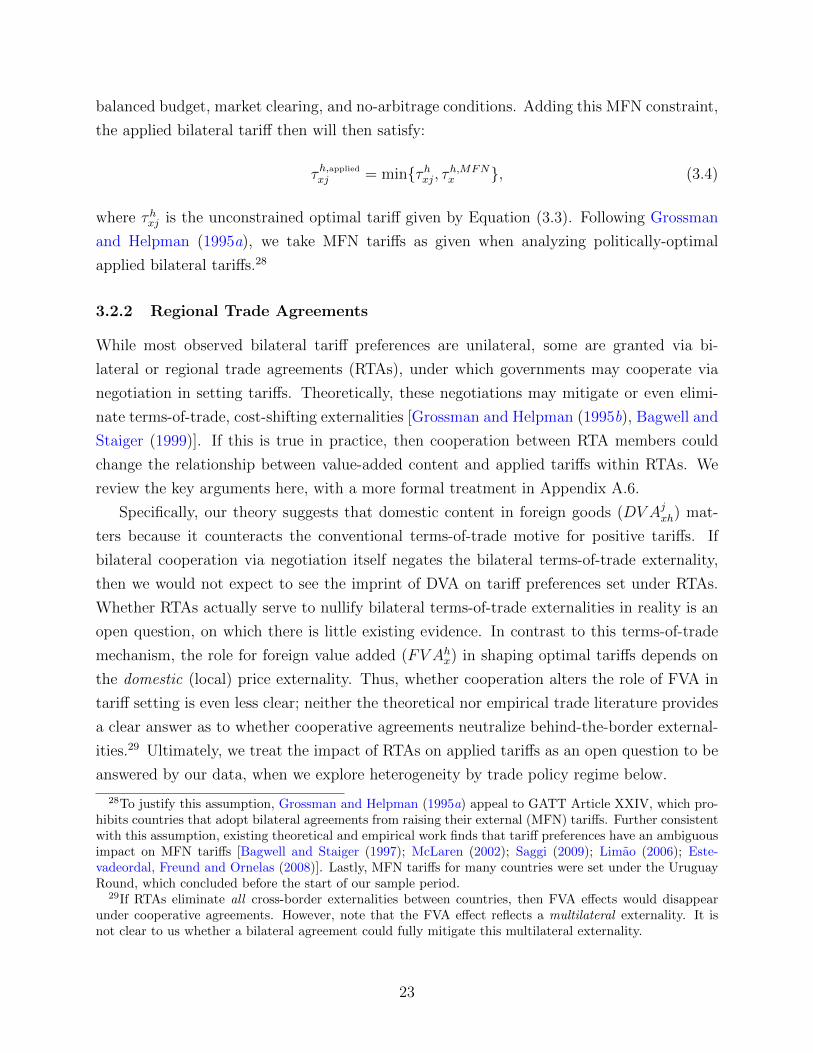
balanced budget, market clearing, and no-arbitrage conditions. Adding this MFN constraint,

the applied bilateral tariff then will then satisfy:

τh,appliedxj = minτhxj, τh,MFNx , (3.4)

where τhxj is the unconstrained optimal tariff given by Equation (3.3). Following Grossman

and Helpman (1995a), we take MFN tariffs as given when analyzing politically-optimal

applied bilateral tariffs.28

3.2.2 Regional Trade Agreements

While most observed bilateral tariff preferences are unilateral, some are granted via bi-

lateral or regional trade agreements (RTAs), under which governments may cooperate via

negotiation in setting tariffs. Theoretically, these negotiations may mitigate or even elimi-

nate terms-of-trade, cost-shifting externalities [Grossman and Helpman (1995b), Bagwell and

Staiger (1999)]. If this is true in practice, then cooperation between RTA members could

change the relationship between value-added content and applied tariffs within RTAs. We

review the key arguments here, with a more formal treatment in Appendix A.6.

Specifically, our theory suggests that domestic content in foreign goods (DV Ajxh) mat-

ters because it counteracts the conventional terms-of-trade motive for positive tariffs. If

bilateral cooperation via negotiation itself negates the bilateral terms-of-trade externality,

then we would not expect to see the imprint of DVA on tariff preferences set under RTAs.

Whether RTAs actually serve to nullify bilateral terms-of-trade externalities in reality is an

open question, on which there is little existing evidence. In contrast to this terms-of-trade

mechanism, the role for foreign value added (FV Ahx) in shaping optimal tariffs depends on

the domestic (local) price externality. Thus, whether cooperation alters the role of FVA in

tariff setting is even less clear; neither the theoretical nor empirical trade literature provides

a clear answer as to whether cooperative agreements neutralize behind-the-border external-

ities.29 Ultimately, we treat the impact of RTAs on applied tariffs as an open question to be

answered by our data, when we explore heterogeneity by trade policy regime below.

28To justify this assumption, Grossman and Helpman (1995a) appeal to GATT Article XXIV, which pro-hibits countries that adopt bilateral agreements from raising their external (MFN) tariffs. Further consistentwith this assumption, existing theoretical and empirical work finds that tariff preferences have an ambiguousimpact on MFN tariffs [Bagwell and Staiger (1997); McLaren (2002); Saggi (2009); Limao (2006); Este-vadeordal, Freund and Ornelas (2008)]. Lastly, MFN tariffs for many countries were set under the UruguayRound, which concluded before the start of our sample period.

29If RTAs eliminate all cross-border externalities between countries, then FVA effects would disappearunder cooperative agreements. However, note that the FVA effect reflects a multilateral externality. It isnot clear to us whether a bilateral agreement could fully mitigate this multilateral externality.

23

3.3 Empirical Strategy

The GVC-augmented tariff theory summarized by Equation (3.3) guides our empirical strat-

egy. To move from this implicit expression for the optimal tariff to a concrete estimation

framework, it is helpful to invoke an approximation argument. We take a linear approxima-

tion around a baseline equilibrium in which there are no GVC linkages (~ν = 0, such that

DV Ajxh = 0 and FV Ahx = 0 ∀x ∈ S, j ∈ C).30 The result is:

thxj =1

εjxh+ γIPxhj

(FGh

xt

phxEjxh

)+ γDV Axhj

(DV AjxhpjxE

jxh

)+ γFV Axh

(FV AhxphxE

jxh

)+ ωxhj, (3.5)

where thxj ≡ τhxj−1, bars denote equilibrium objects evaluated at the point of approximation,

FGhxt ≡ phxq

hx , γIPxhj ≡

δPExεjxh|λ

hxj |

, γDV Axhj ≡ −(1+δDVAx )εrjxh

εjxh, γFV Axhj ≡ −

(1−δFV Ax )εrhx∗εjxh|λ

hxj |

, and ωxhj includes

approximation errors and potential trade diversion effects.31

This expression is a mix of observable variables and parameters that cannot be measured

directly. The three key observables are the levels of final goods production (FGhxt), foreign

GVC income generated by home production (FV Ahxt), and domestic GVC income from

foreign production (DV Ajxht). Each of these is measurable in our data, using the value-

added content of final goods as a proxy for GVC income. In Equation (3.5), each of these

observables is written as a ratio to bilateral imports in the no-GVC equilibrium, which we do

not observe. In forming our estimating equation below, we will use realized bilateral imports

as a proxy for these unobserved values to compute the ratios.32 In terms of language, we refer

to the ratio of domestic final goods production to bilateral imports as the inverse import

penetration ratio, or IP ratio for short. We refer to the ratios of foreign value added and

domestic value added to bilateral final goods imports as the FVA ratio and DVA ratio.

In using these ratios in a regression context, we face two standard, related empirical

challenges. The first is that data for each ratio is positively skewed, with a long right tail.

This right tail variation is difficult to reconcile with (more moderate) observed variation in

30This type of linearization is common in the literature [e.g., Ludema and Mayda (2013)], and Ludemaet al. (2019) adopt a similar point of linearization in a closely related model with GVCs.

31ωxhj ≡ uxhf − Ωxj , where uxhf is the approximation error and Ωxj captures potential trade diversioneffects. Third-country effects are generally ambiguous in sign, and plausibly small, especially for smaller tradepartners that may generate little or no trade diversion; they can be eliminated from the theory by invokingadditional modelling assumptions (e.g., Armington preferences or international market segmentation). Inpractice, our fixed effects also remove importer-industry and exporter-industry characteristics, which likelyabsorbs some of this residual variation.

32Using realized imports here introduces a potential simultaneity problem, where actual imports dependon tariffs, which we will resolve using instrumental variables below. A subtle point is that import quantitiesare evaluated at exporter prices in the first and third ratios and at importer prices in the second. We suppressthis distinction in the empirical work, because we are not able to measure imports at different prices in thesame data set that we use to construct the numerators.

24

tariffs, without resorting to extreme (unobserved) coefficient heterogeneity that neutralizes

these effects. Compounding this issue, the second challenge is that each ratio includes

a variable in the denominator that is potentially measured with error. Specifically, most

observations in the right tail of the ratio distribution have low values for imports. If imports

are measured with error, then variation among right tail observations will be largely driven

by the measurement error itself. We address these issues by taking logs of these ratios in

our empirical estimating equation.

Beyond the ratios, the remaining parameters, including the inverse export supply elas-

ticity (1/εhxj) and parameters underlying the γ-terms in Equation (3.5), are not directly

observed. In prior empirical applications of optimal tariff theory, the inverse export supply

elasticity has been constrained to be importer and industry specific.33 Thus, following this

prior work would suggest an importer-industry fixed effect is sufficient to absorb the inverse

elasticity term. Relaxing this assumption, we also allow for importer-year or importer-

industry-year fixed effects, depending on the specification, as well as exporter-industry-year

fixed effects. Together, these fixed effects absorb plausible variation in the inverse elasticity.

Reflecting the flexibility we allowed in the underlying theory, the coefficients attached

to the ratios in Equation (3.5) are potentially heterogeneous, since they depend on political

economy weights, pass-through elasticities, and the export supply elasticity. These three

objects are not directly observable, estimates of them are not generally available, and they

cannot be computed in the absence of a fully specified quantitative model. Thus, we treat

them as parameters to be estimated. We start by assuming that each coefficient is homo-

geneous in our benchmark estimation, as in γIP = γIPxhj, γFV A = γFV Axhj , and γDV A = γDV Axhj .

From this baseline, we then explore the potential for coefficient heterogeneity across country

pairs and sectors, where the composite effects may differ in economically meaningful dimen-

sions. In exploring data on applied tariff levels, we focus in particular on how the impacts of

DVA across partners differ depending whether preferences are conferred via regional trade

agreements, based on the discussion in Section 3.2.2. Shifting attention to price mechanisms,

we explore whether DVA effects differ systematically across sectors and partners based on

upstream and downstream production differentiation, which are proxies for pass-through

elasticities and export supply elasticities.

Drawing on Section 3.2.1, we recall that applied tariffs are constrained by the MFN

rule. Taking this constraint into account, along with the discussion above, we arrive at the

33Among others, see Broda, Limao and Weinstein (2008), Ludema and Mayda (2013), and Nicita, Olar-reaga and Silva (2018). Extending this literature, Soderbery (2018) provides estimates of bilateral tradeelasticities. While these are difficult to employ directly in our empirical work, due to large measurementerror in the estimates and aggregation issues, Soderbery reports that almost three-quarters of the variationin his bilateral elasticity estimates is explained by importer-product fixed effects. Our combination of fixedeffects would push this explained variation higher.

25

following empirical framework for examining applied bilateral tariffs:

th,appliedxjt − th,MFNxt = minthxjt − t

h,MFNxt , 0, with (3.6)

thxjt−th,MFNxt =Φxhjt+γ

FG ln

(FGhxtIMh

xjt

)+γDV A ln

(DV AjxhtIMh

xjt

)+γFV A ln

(FV AhxtIMh

xjt

)+exhjt, (3.7)

where t denotes the time period, IMhxjt is the value of bilateral imports by h of goods from

sector x in country j, Φxhjt denotes the set of fixed effects, and exhjt is a regression residual.

Noting the sign convention (more generous preferences are associated with more negative

tariffs relative to MFN), theory predicts that γFG > 0 and γDV A < 0. With the prior that

δFV Ax < 1, then we expect γFV A < 0 as well.

We present results for two alternative sets of fixed effects. The first specification includes

importer-industry, importer-year, and exporter-industry-year fixed effects, as in Φxhjt =

φxh + φht + φxjt. Under this specification, we are able to separately estimate all three γ-

coefficients attached to the ratios. In this specification, γFV A is primarily identified based on

multilateral variation in average tariff preferences and foreign value added by importer and

industry over time.34 In contrast, γDV A is identified both by variation across trade partners

for a given importer and industry in the cross section, as well as variation over time.

The second specification includes importer-industry-year and exporter-industry-year fixed

effects: Φxhjt = φxht+φxjt. In this specification, we can identify γDV A, along with a composite

coefficient γFG + γFV A, which is identified by variation in bilateral imports across partners

within a given importer-industry-year cell. Note further that the importer-industry-year

fixed effect differences out multilateral changes in the DVA ratio within each importer and

industry, sharpening the focus on bilateral variation for identification of γDV A. This bilateral

variation is predominantly cross-sectional in nature, as we discuss further below.

A second point worth noting in Equation (3.6) is that we have rewritten the dependent

variable to be the tariff preference, defined as th,appliedxjt − th,MFNxt , with corresponding redefi-

nition of the optimal tariff preference (thxjt−th,MFNxt ). This means that a uniform reduction

in all tariffs leaves the dependent variable unchanged. Further, if only MFN tariffs change,

then tariff preference margins would be compressed. This can be interpreted as a tightening

of the the censoring bound in our empirical setup, and it ensures that changes in MFN tariffs

are not driving our empirical results.35

34More precisely, due to the importer-year fixed effects, identification is based on differential changes acrossindustries within a given importer. Variation in imports across trading partners within a given importer andindustry provides a secondary source of identification, through their impact on the FVA ratio.

35In OLS specifications that do not adjust for censoring, reductions in MFN tariffs (holding th,appliedxjt

constant) bias γDVA and γFV A toward zero, which works against rejecting the null. Note that this redefinitionis redundant with importer-industry-year fixed effects, which absorb all multilateral tariff variation.

26

3.4 Threats to Identification

Assessing threats to identification requires taking a stand on the nature of the regression

residual (exhjt) in Equation (3.7). Because the regression includes proxies or controls for the

key determinants of optimal tariffs suggested by theory, the most straightforward interpreta-

tion of it is that it represents a pure structural error (e.g., measurement error in tariffs) that

is orthogonal to the regressors. In this event, we are estimating an equilibrium relationship

from the model, and we can directly interpret OLS parameter estimates as describing the

optimal policy rule.36

We acknowledge, however, that this structural assumption is strong. So, we seek to

address threats to identification that originate inside the model, as well as potential concerns

that originate outside the model.

Within the model, the key concern is that the residual represents true tariff variation

not explained by the model. In this case, there is a potential simultaneity problem, wherein

the realized values of the ratios on the right-hand side are correlated with the residual. For

example, DV Ajxht depends on the price of foreign output (pjxt), and this price is a function

of country h’s tariff on imports of x from j (thxjt). This mechanism would induce a negative

correlation between ln(DV Ajxht) and ehjxt, which could bias the coefficient estimates. Related

arguments hold for final production, foreign value added, and bilateral imports. In this

multivariate context, with more than one potentially endogenous variable, it is not obvious

a priori which direction the bias would run for individual coefficients, but the overarching

concern is that the coefficients could be biased in directions that would lead us to erroneously

find support for our theoretical predictions.37 To address these simultaneity concerns, we

use an instrumental variables strategy.

Remaining threats to identification lie outside the model. First, there are measurement er-

ror concerns regarding right-hand side variables – e.g., value-added contents are undoubtedly

measured with error. Second, one might reasonably be concerned about omitted variables

that influence both tariffs and value-added content. Because we include the main determi-

nants of tariffs suggested by the theory in our empirical specification, as well as a rich set

of fixed effects, we do not have strong priors about which omitted variables might present

36Note that simultaneity concerns – that true tariffs may influence value-added content, final goods pro-duction, and imports – are not an impediment to estimation of the equilibrium policy rule in this case.

37Taking each partial correlation in isolation, the possible negative correlation between ln(DV Ajxit) and

eijxt would bias the coefficient on ln(DV Ajxit) towards being negative, thus tending to confirm the theory.

On the other hand, the possible positive correlation between ln(FV Ajxit) and eijxt would tend to bias thiscoefficient in the positive direction. This second case of positive bias is less of a concern than the first, becausethe bias would work against confirming the theory. Notwithstanding this intuition, we re-emphasize thatintuition regarding directions of simultaneity bias in the single endogenous regressor case is not necessarilyapplicable in this multivariate context.

27

a threat to identification. Nonetheless, we explore how our results change in response to

adding standard proxies for bilateral relationships.

Having flagged these issues, we defer implementation details to Section 4.3.

3.5 Data

This section briefly describes sources and methods for compiling our data on bilateral tariffs

and value-added content, with full details in Appendix B.1.

Bilateral Tariffs We construct bilateral, industry-level tariffs on final goods for five bench-

mark years: 1995, 2000, 2005, and 2010, and 2015. We start with product-level tariff sched-

ules collected by UNCTAD (TRAINS) and the WTO, which we obtain via the World Bank’s

WITS website. Combining these sources and aggregating product lines yields a data set of

bilateral tariffs at the Harmonized System (HS) 6-digit level. We then identify final goods

(consumption and capital goods) in the data and link HS categories to WIOD industries us-

ing a correspondence developed by the OECD. We take simple averages across HS categories

within each industry to measure industry-level applied bilateral and MFN tariffs.

Value-Added Content of Final Goods Production We use data from the World

Input-Output Database (WIOD) to compute the national origin of value added contained in

the final goods that each country produces, which allow us to construct the empirical coun-

terparts to the domestic and foreign value added terms in the theory. The exact procedure,

which is based on Los, Timmer and de Vries (2015), is described in the appendix. Combining

data from two versions of the WIOD dataset, we are able to construct value-added contents

for 14 “countries” (13 countries, plus the composite EU region) and 14 industries, which are

listed in Table 1, that cover the 1995-2014 period. We use value-added contents from 2014

in our analysis of tariffs in 2015.

3.6 First Look at the Data

Before moving to formal analysis, we pause to discuss sources of variation in the bilateral

tariff data. We then relate observed tariff variation to value-added content in an illustrative

case to fix ideas.

Tariff Preferences Our empirical strategy focuses on differences between bilateral applied

tariffs and applied MFN rates. We start here with a brief summary description of the four

28

main policy regimes under which countries offer lower-than-MFN tariffs to selected trading

partners, with additional discussion in Appendix B.1.

The first regime is the Generalized System of Preferences (GSP), which is an explicitly

unilateral preference regime through which developing countries receive preferential treat-

ment from high-income importers. An important feature of the GSP program is that each

GSP-granting country unilaterally chooses the set of GSP-receiving countries to which and

sectors in which it extends preferences, and these choices differ across GSP-granting coun-

tries and time. Free trade agreements and customs unions, authorized under WTO Article

XXIV, are a second source of preferences. One point worth emphasizing here is that free

trade agreements do not typically entail completely free trade: carve-outs in Article XXIV

agreements are pervasive, and almost half of tariffs imposed on RTA partners are greater

than zero in our data.38 The third source of preferences derives from trade agreements

struck between developing countries under the auspices of the WTO’s Enabling Clause, in-

cluding so-called “Partial Scope Agreements.” Lastly, a handful of idiosyncratic programs

and one-off preferences constitute a fourth source of preferences in our data.

In Figure 1, we track the overall prevalence of tariff preferences, broken down into three

broad categories: RTAs, GSP, and Other (partial scope and miscellaneous). Because our

country panel is imbalanced, we report this break-down of tariff preferences for both the 10

importing countries with data available in all years, alongside the analogous information for

the set of all countries from 2005 onward.

The first point to note is that tariff preferences are widespread: depending on the year,

between 30-40% of all importer-exporter-industry cells have preferential tariffs. The second

point to note is that the prevalence of tariff preferences has been increasing over time,

rising by about ten percentage points from 1995 to 2015. At the same time, because many

preferences remain in place throughout our sample period, the cross-section of preferences

(across sectors and trading partners) is an important source of identifying variation. The

third important feature of the data is that the composition of preferences changes over time.

In general, RTAs and partial scope agreements have become more important sources of

preferences over time, and they seem to progressively displace GSP preferences. Since the

magnitude of tariff preferences is generally larger under RTAs and partial scope agreements

than under the GSP, this policy substitution represents a deepening of preferences over time.

Case Study: Textiles, Leather, and Footwear Before moving to the full empirical

estimation, we briefly introduce data for the Textiles, Leather, and Footwear sectors, where

38As Estevadeordal, Freund and Ornelas (2008) put it: “Article XXIV is . . . perhaps the least enforcedarticle of the GATT, and in reality the complete elimination of internal tariffs is the exception, rather thanthe rule, in most operative RTAs.” For analysis of RTA coverage by the WTO Secretariat, see WTO (2011).

29

value chain linkages are salient to policymakers, and the scope for and use of tariff discretion

is high. We examine two simple manipulations of the data, both to fix ideas and to highlight

the sources of identifying variation we exploit in the empirical analysis.

We start by examining the relationship between FV A and average tariff preferences,

focusing on long-differences within importer-industry cells. Define the (multilateral) mean

tariff preference by importer and industry as tixt = 1C−1

∑j 6=i

(tixjt − t

i,MFNxt

), with corre-

sponding change over time ∆ttixt.

39 Figure 2 plots ∆ttixt against changes in the (log) FVA

ratio – defined as ∆t ln(FV AixtIM i

xt

)– by importer and industry, from 1995 to 2015. As is evident

in the figure, there is a negative correlation in the data, consistent with theory: countries

that saw comparatively more growth in FV A relative to gross imports also offered the great-

est expansion of preferential market access to their trading partners.40 This type of time

series variation by importer and industry will be used to identify FVA effects, which are

fundamentally multilateral in nature, as discussed in section 3.1.

Next we examine the relationship between DV A and bilateral tariff preferences, focusing

on the cross-sectional dimension of the data. Honing in on a set of high-income importers

buying goods from a set of emerging-market exporters, Figure 2 plots bilateral tariff pref-

erences (tixj − ti,MFNx ) against the (log) DVA ratio [ln

(DV AixjtIM i

xt

)] by country-pair in 2015.41

We note three key points in the figure. First there is a negative correlation between applied

tariffs and the DVA ratio, consistent with theory: high-income importers offered more gen-

erous tariff preferences for imports of Textiles, Leather, and Footwear to emerging-market

trading partners that use more of their own value-added inputs in production of those goods.

Second, there is sizable variation in tariff preferences (on the y-axis) and the (log) DVA ratio

across partners (on the x-axis). This type of cross-sectional variation is the main source of

identification for the role of DVA in our empirical estimation. Lastly, there is an obvious

censoring problem in the figure, as indicated by the mass of country pairs with zero prefer-

ence. This censoring may bias the simple correlation toward zero, so we adjust for it in the

empirical work that follows.

39Changes in mean tariff preferences are driven both by expansion in the number of countries receivingpreferences over time, and changes in the average depth of preferences.

40One particular feature of the Textiles, Leather, and Footwear sectors is that most importers experiencedeclines in their FVA ratios over time, due to imports rising faster than FVA (which is also rising in absoluteterms for most countries). Our estimation exploits differences in these changes across sectors and countries,rather than the absolute level of these changes.

41We construct comparable sets of importers and exporters to mimic the role of importer-industry andexporter-industry fixed effects in the analysis.

30

4 Results I: Tariffs and GVCs

We present results for tariffs in three steps. First, we present a baseline specification in

Section 4.1, in which we use OLS and Tobit regressions to describe how applied and optimal

tariffs are related to value-added content under the assumption that effects are homogeneous

across country pairs and sectors. We then pivot in Section 4.2 to examine heterogeneity in

responses, depending on the trade policy regime under which tariff preferences are conferred

and the sectors in which they occur. We then address threats to identification in Section 4.3,

by appealing to instrumental variables and incorporating additional control variables into

the empirical specification.

4.1 Baseline Specification

We present estimates of Equations (3.6)-(3.7) in Table 2. In all columns, the dependent

variable is the observed tariff preference: th,appliedxjt − th,MFNxt . In columns (1)-(2), we present

OLS results, ignoring censoring induced by the MFN rule. In columns (3)-(4), we present

Tobit estimates that adjust for censoring. In columns (1) and (3), we include importer-year

and importer-industry fixed effects, which allows us to identify the coefficient attached to

the ratio of FVA to bilateral imports (γFV A) separately from the coefficient on the import

penetration ratio (γIP ). In columns (2) and (4), we include importer-industry-year fixed

effects, where we can only identify the joint coefficient γFV A + γIP , identified from bilateral

variation in imports. Note that theory does not restrict the sign of this joint coefficient, so

we do not seek to interpret its estimated sign or statistical significance.42 Exporter-industry-

year fixed effects are included in all specifications, and all columns feature standard errors

that are clustered by importer-exporter pair.

In column (1), we see that the OLS coefficients on the DVA ratio is negative: applied

bilateral tariffs are lower (tariff preferences are larger) when the bilateral DVA ratio is high,

consistent with the theoretical prediction. The coefficient is little changed in column (2),

where we add an importer-industry-year fixed effect to hone in on variation across bilateral

partners. To interpret the magnitudes, it is typical for the DVA ratio to vary by 5 log points

across exporters within a given importer and industry.43 The point estimate in column (1) is

about −1, so moving from low to high DVA partners corresponds to roughly a 5 percentage

point reduction in observed applied tariffs. Since the median tariff is around 8 percent in

our data, this represents a substantial expansion of market access.

42Although the joint coefficient need not be exactly equal to the sum of the γFV A and γIP from thespecification with importer-industry and importer-year fixed effects, we find it is typically quite close.

43This is the median difference between maximum and minimum values across the 13 trading partners ineach importer-industry-year cell.

31

In column (1), applied bilateral tariffs are also lower when the multilateral FVA ratio is

larger, consistent with political economy forces being relatively weak (δFV Ax < 1). Focusing

on time variation, some sectors see increases in the FVA ratio over time, with typical values on

the order of 1 log point, while others see declines, with typical values of -1 log points. These

differential changes lead to declines of about 2 percentage points in mean tariff preferences

in sectors with growing FVA ratios relative to those with falling FVA ratios.

As a final point to note in column (1), the coefficient on the IP ratio is positive: a higher

ratio of domestic final goods production to imports (or a lower import penetration ratio)

is associated with higher tariffs, consistent with the government having stronger political

economy incentives to protect domestic producers in this case. While this coefficient is of

secondary interest to us as a control variable, we note that these estimates are consistent

with empirical findings in the existing literature [Goldberg and Maggi (1999); Gawande and

Bandyopadhyay (2000)].

Turning to Tobit estimates of the same specification in column (3), we see that adjusting

for censoring pushes both the coefficients on the DVA ratio and FVA ratio away from zero,

roughly doubling the size of the estimated coefficients. This is consistent with our interpreta-

tion that MFN tariffs represent a constraint on countries’ use of bilateral discretion in tariff

setting. Put differently, optimal tariffs appear to be more sensitive to value-added content

than are actual applied tariffs.

4.2 Exploring Heterogeneity

With a baseline established, we now turn to alternative cuts of the data that explore het-

erogeneity in our results based on the nature of preferences and underlying economic forces

that could shape how GVC linkages influence tariff setting. We explore heterogeneity across

trade policy regimes in Section 4.2.1 and by degrees of upstream and downstream product

differentiation in Section 4.2.2.

4.2.1 Trade Policy Regimes

As discussed in Section 3.6, preferences are granted under different policy regimes in our data,

including RTAs, the GSP, and other miscellenous preference programs. Further, building

on Section 3.2.2, preferences granted through RTAs may reflect cooperation, potentially

displacing DVA effects within those agreements. Thus, we turn to parsing out the role of

trade policy institutions.

To begin, we replicate our baseline estimation including an additional indicator variable

RTAhjt that takes the value one when countries h and j have a regional trade agreement

32

in place at date t. The coefficient on RTAhjt is the (conditional) mean difference in tariffs

between pairs with and without an RTA in place, thus it removes some of the variation in

bilateral tariffs available for estimation of DVA and FVA effects. Nonetheless, in Panel A of

Table 3, we continue to find negative and significant coefficients on both the DVA and FVA

terms under both OLS in columns (1)-(2) and Tobit in columns (3)-(4).

Reflecting the fact that there is diminished residual variation after controlling for RTAs,

the estimated coefficients are smaller (in absolute value) in Panel A than in the baseline

(Table 2). This is expected. First, the RTA indicator removes considerable cross-sectional

variation, which is the main source of identifying variation for the DVA effect; in essence, the

RTA indicator supplants the role for DVA in predicting which bilateral pairs form RTAs, thus

conferring each other the largest preferences. It also has important implications for the FVA

coefficient. FVA effects are primarily identified by changes in mean tariffs by importer and

industry over time. Since the RTA indicator removes the average reduction in applied tariffs

due to RTA adoption, it absorbs the impact of progressive RTA expansion over our sample

period (depicted in Figure 2) on mean importer-industry preferences. Thus, by including the

RTA indicator we discard important time series variation for identification of FVA effects.

Turning to Panel B in Table 3, we interact each right-hand side variable with the RTA in-

dicator, which allows us to estimate heterogeneous coefficients by type of preference. The mo-

tivation for this specification follows the discussion in Section 3.2.2: if RTAs completely neu-

tralize the bilateral terms-of-trade externality, then DVA should not influence tariffs set un-

der RTAs, meaning that the coefficient on the interaction term RTAhjt× ln(DV Ajxht/IMhxjt)

should be zero. At a minimum, we expect diminished sensitivity of tariffs to DVA if RTAs at

least partially neutralize the bilateral terms-of-trade externality. Assuming that δFV A < 1,

we expect to find that the coefficient on the FVA ratio is negative for tariffs set both within

and outside regional agreements, since its impact reflects a local price externality that is

multilateral in scope (see Section 3.2.2).

Comparing the results in the first and second rows of Panel B, we find that the coefficient

on the DVA ratio within RTAs is not statistically different from zero in any specification,

and it is meaningfully smaller than the estimated coefficient outside RTAs across the board.

Further, the coefficient on the FVA ratio is negative and significant both within and outside

RTAs, consistent with theory. It is striking that FVA effects are so strong inside RTAs,

despite null results concerning DVA effects inside the same set of RTAs.

In Table 4, we focus attention entirely on non-RTA preferences, dropping all observations

with RTAhjt = 1 from the estimation. In Panel A, we repeat the baseline estimation in this

sub-sample; we find negative coefficients attached to the DVA and FVA ratios, although they

are attenuated in magnitude in this sample where preferences are less generous on average.

33

To explore preference setting under the GSP program versus partial scope agreements

and other miscellaneous programs, we define the set of potential GSP-granting countries as

those that granted GSP access to at least one other country (at any time) in our sample.44

Likewise, we define the set of potential GSP-eligible countries as those that received GSP

access from at least one other country (at any time) in our sample. We then define an

indicator that identifies which country pairs are potentially eligible for GSP preferences:

GSPij = 1 (i ∈ GSP-granting, j ∈ GSP-eligible). For country pairs with GSPij = 1, the GSP

program itself accounts for essentially all observed preferences in this non-RTA subsample of

the data, in large part because advanced countries have limited scope under WTO rules to

confer preferences outside of RTAs.45 For country pairs with GSPij = 0, non-GSP preference

schemes are the source of observed tariff preferences.

In Panel B of Table 4, we split coefficients based on whether a given country pair could

potentially have a GSP program in place. We find that higher DVA ratios are associated

with lower bilateral tariffs both inside and outside the GSP scheme. For GSP-eligible pairs,

this pattern is apparent only when we adjust for censoring, which is quite sensible given that

the advanced countries that grant GSP preferences generally also have very low MFN tariff

bindings; thus there is strong censoring in this subset of the data. We also see that higher

FVA ratios are associated with lower tariffs among non-GSP country pairs, where partial

scope agreements are the most important source of preferences. We do not find significant

effects of FVA within GSP-eligible pairs. Recalling that FVA effects are identified in large

part based on time variation at the importer-industry level, this is not surprising. The

relatively static nature of the GSP program implies there is limited time series variation

among this group; further, GSP arrangements are replaced by other agreements over time

(see Figure 1), so attrition may also work against finding sharp results here.

44Each GSP-granting country has discretion over the set of countries and sectors included in its GSPprogram, as well as the level of its tariff preferences. In our data, we observe only a uniform tariff preferenceapplied to all countries included in each importer’s GSP program. In reality, countries have scope to varytariff preferences bilaterally, via discretionary application of limits on GSP access (e.g., competitive needslimitations); see Blanchard and Hakobyan (2014). We do not observe these bilaterally targeted preferences,and so our data likely understate the true degree of discretion that countries exercise. As such, one mightexpect our results to be attenuated.

45Many pairs with GSPij = 1 have no recorded bilateral preferences (i.e., j receives MFN treatment fromi), because some potentially GSP eligible exporters are excluded by GSP-granting countries. For example,the US does not grant China preferences in its GSP program, while the EU does. Therefore, while bothGSPUSA,CHN = 1 and GSPEUN,CHN = 1, we observe tariff preferences in only the EUN-CHN case. GSP-granting countries are also able to exclude entire sectors from their GSP programs. Further, GSP scheduleschange over time for some importers, though there is strong persistence over time for most country pairs.

34

4.2.2 Upstream and Downstream Differentiation

In this section, we examine heterogeneous effects that are mediated by pass-through and

trade elasticities in the model. We focus on documenting heterogeneous responses of tariffs

to DVA, where we can use bilateral variation for identification. Referring back to Equation

(3.5), the coefficient attached to the DVA ratio is γDV Axhj ≡ −(1+δDVAx )εrjxh

εjxh. In the numerator,

εrjxh is the elasticity of pass-through from downstream price changes to upstream returns

to value-added inputs. In the denominator, the export supply elasticity (εjxh) may also

be heterogeneous.46 We appeal to first principles to organize this heterogeneity based on

differences in product differentiation across across upstream and downstream sectors.47 We

discuss each in turn.

Upstream Differentiation The theory highlights the important role of pass-through elas-

ticities, embodied in εrjxh, in mediating the relationship between GVC linkages and tariffs. All

else equal, sectors in which final goods prices are more closely linked to the returns to GVC

inputs should see a more pronounced (inverse) relationship between GVC income and tariffs.

We now invoke a simple argument about product differentiation in upstream sectors to think

about sources of variation in εrjxh. We sketch the argument here, and discuss implementation

further in Appendix B.2.

Pass-through elasticities may differ across country pairs because upstream sectors differ

in the responsiveness of input prices to downstream output prices, and the composition of

sectors that supply GVC inputs to downstream producers may differ across bilateral partners.

For example, suppose that country h supplies a commodity (e.g., oil) and a differentiated

manufactured input (e.g., electronic components) to downstream industry x in countries

j and k. All else equal, we would expect returns to the commodity input to be relatively

insensitive to changes in output prices for individual downstream producers that use it, while

the returns to specialized inputs are likely to be sensitive to downstream product prices.

Thus, if country h supplies predominantly commodity inputs to industry x in country j, but

supplies predominantly differentiated inputs to industry x in country k, we would expect the

pass-through from pjx to h’s GVC income to be relatively low compared to the pass-through

from pkx; i.e. εrjxh < εrkxh.

Based on this argument, we decompose domestic value-added in foreign production

46We omit discussion of political economy weights because we lack clear proxies for them. See Ludemaet al. (2019) for evidence on political economy motives in the GVC context.

47While it would be ideal to use direct empirical estimates of these elasticities to discipline the analysis,this is not feasible in practice. Estimating these heterogeneous elasticities is outside the scope of our analysis,while off-the-shelf estimates of pass-through elasticities do not exist, and existing estimates of export supplyelasticities are both noisy and ill-suited to the aggregated industry dimension of our data.

35

(DV Ajxh) based on whether it originates in upstream industries that are plausibly differ-

entiated or nondifferentiated. We do this two ways. First, we simply treat value added

originating in the manufacturing sector as differentiated, and value added originating in the

nonmanufacturing sector as non-differentiated. This is crude, but transparent. Second, we

use the classification developed by Rauch (1999) to compute the share of value added from

each upstream industry that is differentiated versus nondifferentiated. In both cases, adding

up over upstream industries yields bilateral measures for DVA originating in differentiated

upstream sectors (DV Aj,Diffxh ) versus undifferentiated sectors (DV Aj,NonDiffxh ). We then form

DVA ratios with each of these components and repeat our baseline estimation.

We report results for this exercise in Panel A of Table 5, where all columns include

importer-industry-year fixed effects. Columns (1)-(2) report coefficients for the manufactur-

ing versus non-manufacturing split of upstream value added, whereas columns (3)-(4) report

results using the Rauch classification. In all columns, we see that tariffs respond strongly

to DVA originating from differentiated upstream industries, but are weakly related to DVA

originating in non-differentiated industries, as expected.

Downstream Differentiation Turning our attention to downstream industries, export

supply elasticities (εjxh) tend to be correlated with measures of product differentiation [Broda,

Limao and Weinstein (2008)]. To the extent that more differentiated (downstream) industries

are characterized by lower trade elasticities, the theory predicts that tariffs in these sectors

should be more responsive to GVC linkages. Thus, we can also examine heterogeneity in

γDV Axhj across downstream industries (x) based on their degree of production differentiation.

We again consider two alternative classifications. We first allow for heterogeneous coef-

ficients on the DVA ratio for manufacturing versus nonmanufacturing industries. With the

prior that manufacturing is differentiated while nonmanufacturing is not, we expect tariffs to

respond more strongly to DVA in manufacturing. We then classify final goods sectors based

on the Rauch classification, where we define a downstream industry to be differentiated if

more than 50% of the underlying SITC categories in it are differentiated.

In Panel B of Table 5, we re-estimate the baseline model with importer-industry-year

fixed effects, splitting coefficients across sectors based on whether they are differentiated or

undifferentiated. In all cases, the coefficient on the DVA ratio is negative, suggesting that

tariffs respond to value-added content in both sector groups. However, the coefficient for

differentiated downstream industries tends to be larger (in absolute terms) in differentiated

industries. This is most strongly true for the Rauch-based split, where we can reject equality

of the coefficients at the 1% level. This evidence is broadly consistent with the basic economic

forces in our model.

36

4.3 Instruments and Additional Controls

This section addresses the threats to identification that we identified in Section 3.4. We

address simultaneity and omitted variable bias concerns in tandem, using a combination of

instruments and additional controls.

At the outset, we emphasize that the nature of the empirical strategy and data present

formidable challenges for instrumental variables analysis. First, our baseline OLS estima-

tion, based on Equation (3.7), includes multiple potentially endogenous variables, which are

correlated among themselves for legitimate economic reasons.48 Second, because we include

fixed effects in all specifications, there is less residual variation available for us to use in iden-

tification.49 Our task is thus to find instruments that isolate sufficient independent variation

in potentially endogenous variables, conditional on an already-rich set of fixed effects. Third,

because some right-hand side variables are correlated among themselves, we anticipate that

instruments for them might also be correlated among themselves, which presents another

challenge to finding multiple strong, plausibly exogenous IVs.

Given these challenges, it is useful to partition the instrumental variables analysis into two

components, based on the two alternative fixed effects specifications we have used thus far.

First, conditional on including an importer-industry-year fixed effect, we seek instruments

for DV Ajxht and IMhxjt. Second, when we replace the importer-industry-year fixed effect with

importer-industry and importer-year fixed effects in order to use time series variation within

importers and industries to identify the FVA effect, we need to add instruments for FV Ahxt

and FGhxt as well. We discuss instruments and present results in this order.

DVA and Imports The instrument selection problems for domestic value added and im-

ports are related, in that both are bilateral variables and they are correlated with each other.

We need two valid instruments (conditional on controls) that induce sufficient independent

variation in DVA and imports to identify the coefficients.

The first instrument is targeted at breaking the potential simultaneity problem between

DV Ajxht and any residual variation in tariff preferences contained in exhjt. One potential

instrument is to use DV A in an outside sector z 6= x, which is not directly a function

48At the bilateral level, non-tariff bilateral trade costs may influence both bilateral DVA content and finalgoods imports. At the industry level, the level of foreign value added is mechanically related to the level offinal goods production.

49Note that we do not include bilateral (importer-exporter) fixed effects in any specification, becausemany bilateral preferences schemes are present throughout our data (see Figure 1). Removing the bulk ofvariation attributable to these schemes via bilateral fixed effects leaves us with scarce residual variation touse in identifying DVA effects. In effect, we risk throwing out the baby with the bathwater; it is not clearto us that this within transformation would improve identification, particularly when we can control forobservable proxies for omitted variables directly in the empirical specification. Further, the theory does notdirectly support the inclusion additional fixed effects.

37

of thxjt and thus plausibly uncorrelated with exhjt. In what follows, we adopt the services

sector as this outside sector (itself not subject to tariffs), and we refer to this instrument

as DVA-in-Services. As a concrete example, the identification assumption is then that the

amount of US value-added content used in India’s service sector is not determined by the US

import tariff on textiles from India, controlling for remaining observables and fixed effects.

This instrument is likely to be relevant, due to common supply-side factors that make h an

attractive input supplier for j across many sectors, including services.

The main threat to the exclusion restriction derives from potential spillovers across sec-

tors, whereby a reduction in tariffs in sector x could change demand for output in sector z,

which could feed back into DV Ajzht. While possible, we think this is unlikely to be a substan-

tial concern for three reasons. First, services sector output is largely non-traded, and thus

dependent on domestic demand in country j; as such, any spillover channel that operates

through the impact of tariffs on bilateral imports by h from j is likely to be weak. Second,

the direction of this potential spillover is unclear ex ante, and may differ across sectors, so it

seems reasonable to expect such spillovers to be small on average. Third, any potential for

spillover effects to contaminate the estimation is mitigated by the inclusion of an exporter-

industry-year fixed effect in all specifications. This fixed effect purges the instrument of all

exporter-year variation and therefore implicitly controls for the level of services output in

the destination, which would be the main channel through which spillovers would operate.

To instrument for bilateral imports, we exploit heterogeneity in the distance elasticity

of trade across sectors. Specifically, we construct the instrument by interacting the (log)

bilateral distance across trading partners with an indicator that takes the value 1 if industry

x has a high distance elasticity of trade.50 We then control directly for log bilateral distance in

the second stage, ensuring that we use only heterogeneity in distance effects for identification.

This instrument is well-suited to identify bilateral variation in imports that is independent

from DVA, because the distance elasticity of imports varies across sectors, while the distance

elasticity of bilateral DVA content largely does not. The instrument is valid under the

assumption that the direct influence of distance on tariffs (if any) is homogeneous across

sectors, conditional on the remaining observables.51

50We partition industries into high/low groups based on distance elasticities obtained from gravity regres-sions with importer-industry-year and exporter-industry-year fixed effects. These distance elasticities rangefrom −1.5 to −1, and we assign industries with distance elasticities less than −1.25 to the high elasticitygroup; for this group, we cannot reject equality between each industry’s distance elasticity and the highestdistance elasticity sector. These industries are all plausibly heavy, low value-to-weight goods that may becostly to ship long distances: Agriculture and Natural Resources (1), Pulp and Paper Goods (7), Rubberand Plastics (10), Basic and Fabricated Metals (12), and Transport Equipment (15).

51While we believe this assumption to be credible, we discuss an alternative strategy to instrument forimports in Appendix B.2, which yields similar results.

38

FVA and FG In our specifications with importer-year fixed effects, we design shift-share

instruments for FV Ahxt and FGhxt, which combine observed cross-sectional variation at the

beginning of our sample with plausibly-exogenous growth patterns. This approach allows

us to exploit just the plausibly-exogenous component of inter-temporal variation in FG and

FVA across sectors.

Specifically, we use a “pull” instrument for FGhxt, which for each importer h interacts

the share of final output in industry x sold to each destination j in the base year (1995)

with subsequent growth in destination-specific expenditure on industry x. Correspondingly,

we construct a “push” instrument for FV Ahxt. Let FV Ahzxj0 be value added from upstream

sector z in country j used by industry x in country h in the base year, with FV Ahx0 =∑j 6=h∑

z FV Ahzxj0. Then we interact these bilateral FVA sourcing shares with foreign value-

added growth in upstream sectors to form the instrument. The instruments take the form:

ln FGh

xt = ln

(∑j

(FGh

xj0

FGhx0

)FGxjt

FGxj0

)(4.1)

ln F V Ah

xt = ln

(∑j 6=h

∑s

(FV Ahj0(s, x)

FV Ahx0

)V Ajst

V Ajs0

)(4.2)

Controls In addition to the instruments described above, we also add additional control

variables to address concerns about potential omitted variables bias. While theory does not

present us with guidance about which controls might be necessary to add to the regression,

we consider conventional bilateral controls used in the empirical trade literature. As noted

above, all specifications will include (log) bilateral distance as a control variable. We also

include colonial history, common language, and a common border (contiguity).52 These

controls have been shown to predict the adoption of bilateral trade agreements (RTAs) in

previous work by Baier and Bergstrand (2004) and Egger et al. (2011), so are reasonable

controls for determinants of bilateral preferences more generally.

Results We present results with these instrumental variables and additional controls in

Table 6. Panel A reports results from specifications that include importer-industry-year

fixed effects, in which only the instruments for DV Ahxjt and IMhxjt are used. In column

(1), we report OLS estimates that control for bilateral distance.53 In columns (2)-(4), we

52We obtain these variables from the CEPII GeoDistance Database: http://www.cepii.fr/CEPII/fr/

bdd_modele/presentation.asp?id=6. Bilateral characteristics for the EU are defined using GDP-weightedaverages of bilateral characteristics for each individual EU country; thus, colonial linkages, common language,and contiguity are not strict indicator variables when the EU is a trading partner.

53The direct effect of distance is positive, while γDVA and γIP + γFV A are somewhat diminished relativeto the comparable estimates in column (2) of Table 2. Interpreting this result requires care, because we

39

report instrumental variables results. The first take-away is that the coefficient attached to

the DVA ratio is negative in all specifications, and larger in absolute value than the OLS

baseline. The second result is that this DVA coefficient is relatively stable with introduction

of auxiliary bilateral control variables. Note that the estimate of γIP +γFV A is driven toward

zero in these specifications; we have little to say about this, since theory does not make a

prediction for the value of this sum.

In Panel B of Table 6, we report results for specifications with importer-industry and

importer-year fixed effects, in which we can estimate γIP and γFV A separately, as well as

γDV A. The headline result is that the coefficient on the FVA ratio is negative in the IV

estimation while the coefficient on the inverse import penetration ratio is positive, and the

instrumental variables estimates are generally larger in absolute value than the commensu-

rate OLS estimates. The coefficients on the FVA and IP ratios are significant at conventional

levels in columns (6) and (7), but weaker in column (8) when we control for regional trade

agreements (as discussed earlier, removing variation attributable to RTAs significantly re-

duces the inter-temporal variation available for identification of these coefficients).54

These instruments perform relatively well despite the challenges identified above.55 In

Panel A, the instruments pass rule-of-thumb thresholds (test statistics greater than 10),

so conventional standard errors are likely appropriate. In Panel B, the case is less clear-

cut based on the Wald rk F-statistic test for weak identification, though the conditional

F-Statistics exceed rule-of-thumb thresholds. Thus, while we present conventional standard

errors in parentheses in Panel B, we also provide weak-IV robust confidence intervals in

brackets for the key coefficients.56

Supplemental IV Results In Appendix B, we “stress test” the IV strategy described

above in several ways. First, we consider an alternative instrument for imports, based on

have introduced a control variable that is naturally correlated with the remaining right-hand side variables;the coefficient on bilateral distance may be positive either because it directly matters for tariff setting, orbecause it is correlated with the DVA ratio and IMh

xjt. Put differently, γDVA and γIP +γFV A now estimatethe influence of only the variation in the DVA ratio and imports that is not explained by bilateral distanceon preferential tariffs. Some of the variation that is “partialed out” by bilateral distance may in fact be“good variation” that is informative about the theory.

54The RTA indicator removes the impact of the spread of RTAs on mean preferences at the importerand industry level, which reduces the time series variation available to estimate γFV A and γDPE . From atheoretical perspective, FVA and domestic political economy should influence preferences both inside andoutside RTAs, so there is not a strong ex ante argument to control for RTAs in this specification. Thus,while discarding this variation pushes γFV A and γDPE toward zero, this is not the preferred estimate.

55There is little guidance in the literature about appropriate critical values to use in screening for weakinstruments with multiple instruments and clustered standard errors [Andrews, Stock and Sun (2019)].

56These confidence intervals are based on the projection method, applied to the conditional likelihoodratio (CLR) test statistic with nominal size of 10%. They are also conservative, in that these intervals coverthe true value with probability that is strictly higher than the size of the test.

40

values of bilateral imports that are predetermined with respect to tariffs observed in our

data, which replaces the heterogeneous distance effects instrument used above. Second, we

separately consider an alternative instrument for DV Ahxjt, again based on predetermined

values of bilateral DVA in 1970. While this alternative DVA instrument contains useful

variation and delivers consistent qualitative results, it is weak in some specifications, and so

requires separate discussion. Nonetheless, we show in the appendix that the core IV results

are robust to these permutations.

5 Results II: Temporary Trade Barriers and GVCs

In addition to bilateral applied tariffs, governments use non-tariff barriers to restrict imports.

In this section we examine whether GVC linkages influence these polities as well. We focus

on a specific class of these barriers, known collectively as temporary trade barriers (TTBs),

which include antidumping, safeguards, and countervailing duties. These policies are both

directly observable and politically salient trade policy instruments in the modern economy.

Temporary trade barriers are a natural testing ground for the GVC mechanisms indicated

by theory. Countries have wide latitude under WTO rules to use TTBs, and they can be

targeted at particular trading partners and products. For countries with low MFN tariffs,

TTBs are one of the few WTO-consistent means by which to implement discriminatory trade

policy, and accordingly, their use has been rising over time [Bown (2011)]. Prior research has

found that non-tariff barriers generally, and TTBs specifically, appear to respond to optimal

tariff considerations, which suggests TTBs may offer fertile territory for exploring the effects

of DVA in particular.57

Data and Empirical Strategy We obtain data on temporary trade barriers (TTBs)

– antidumping, safeguards, and countervailing duties – from the World Bank’s Temporary

Trade Barriers Database [Bown (2016)]. These data identify the importing country imposing

the TTB, the countries and product lines on which the TTB is imposed, and the timing of

when TTBs are imposed and removed. Following Trefler (1993) and Goldberg and Maggi

(1999), among others, we construct import coverage ratios, which measure the stock of

accumulated bilateral TTBs imposed by each importer against individual exporters in each

57Broda, Limao and Weinstein (2008) find that US NTBs are higher in sectors with high inverse exportsupply elasticities. Bown and Crowley (2013) find that United States’ use of antidumping and safeguardsis consistent with the Bagwell and Staiger (1990) model of self-enforcing trade agreements and cooperativetariffs. Trefler (1993) also used US NTB data in studying endogenous trade policy, and Goldberg and Maggi(1999) and Gawande and Bandyopadhyay (2000) used US NTB data in their empirical examination of theprotection-for-sale model [Grossman and Helpman (1994)].

41

industry and year. See Appendix B.1.3 for further data details.

In examining TTB use, our empirical specifications follow the approach for applied tariffs

with two modifications. First, instead of measuring the downward deviation of applied

bilateral tariffs from MFN tariffs, our dependent variable now measures the coverage ratio:

the share country h’s imports from trading partner j that face a positive TTB in a given

year and sector. These coverage ratios follow the same sign conventions we used for bilateral

tariffs: lower coverage ratios are associated with lower trade protection. Second, we use

lagged measures of value-added content in our regressions, since the TTB import coverage

ratio (the dependent variable) measures the stock of TTBs in force, rather than the flow of

new TTBs imposed/removed. Because TTBs typically remain in effect for a number of years,

many TTBs in effect at date t were actually imposed in previous periods. Therefore, lagged

value-added content better captures the information that was relevant to policymakers at

the time when barriers currently in effect were actually adopted.

Results Table 7 presents ordinary least squares estimates for TTB coverage ratios.58 Con-

sistent with previous tables, columns (1) and (3) include results with importer-year, industry-

year, importer-industry, and exporter-industry-year fixed effects, while columns (2) and (4)

include importer-industry-year and exporter-industry-year fixed effects. We find that both

higher levels of domestic value added in foreign production and foreign value added in do-

mestic production are associated with lower TTB coverage ratios. Governments appear to

curb their protectionist TTB actions where value chain linkages are strongest. Further, the

coefficient on the inverse import penetration ratio is positive. These results are broadly

consistent with our results for tariffs.59

Finally, it would be remiss in any analysis of TTBs to overlook the outsize role played

by China. In our data, China is the exporter in approximately 30 percent of the importer-

exporter-industry-year cells in which TTBs are observed as being used (i.e., with non-zero

coverage ratios), roughly three times as many as the next highest exporter. Further, it is

very rare during this particular time period for countries to impose TTBs in a given sector

without also including China among the set of exporters on which barriers are imposed

58Although TTB coverage ratios have a mass point at zero, several arguments lead us to opt for OLS toanalyze them, rather than limited dependent variable methods. First, positive values are relatively rare inthe data, occurring in only 6 percent of our importer-exporter-industry-year cells. Binary outcome models(e.g., Probit and Logit) are potentially biased in this context [King and Zeng (2001)]. Further, for Tobitmodels, the distribution of the rare positive outcomes is constrained to follow the extreme upper tail of thenormal distribution, which seems untenable in our context. Second, as a practical matter, standard censoringarguments suggest that OLS coefficients of interest would be biased toward zero. Thus, OLS is a robust andlikely conservative approach to characterizing our data.

59In the table, we cluster on importer-exporter-industry, because TTB policy decisions are independentacross industries. The inferences we draw are robust to clustering by importer-exporter pair instead.

42

[Bown (2010), Prusa (2010)]. At face value, these observations suggest that most of the

TTB use during this period is aimed at China. Recognizing this possibility, we separately

examine how bilateral value-added content influences TTB use depending on whether China

is the exporting country. To this end, we interact the DVA measure with an indicator for

whether China is the exporter, and then re-estimate the specifications from Panel A. (Since

both FV A and FG are multilateral (not bilateral), we have no a priori expectation that

they should impact TTB use against China differently from TTB use writ large.)

The results are reported in Panel B of Table 7. The main finding is that TTB coverage

ratios are substantially more sensitive to DVA content when China is the exporter. There

is some evidence for similar targeting for non-Chinese exporters in column (3), but it is

substantially weaker. Thus we conclude that importers seem to target TTB use against

China in a manner that shields their own upstream suppliers from harm.

6 Conclusion

This paper introduces a new value-added approach for exploring the role of global value

chains in shaping trade policy. Fundamentally, GVCs erode the link between the location

in which final goods are produced and the nationality of the value-added content embodied

in those goods. Because import tariffs are by definition applied based on the location where

goods are made, GVCs modify optimal tariff policy.

When domestic content in foreign final goods is high, governments have less incentive to

manipulate the (final goods) terms-of-trade, leading to lower import tariffs. When foreign

content in domestic final goods is high, some of the benefits of protection are passed back

up the value chain to foreign suppliers. This mechanism further lowers optimal tariffs. We

find evidence in support of both of these predictions in two distinct empirical settings: when

countries discriminate across trading partners by lowering protection through bilateral tariff

preferences, and when countries discriminate by raising protection through the adoption of

temporary trade barriers. These results demonstrate the empirical importance of specific

channels through which global value chains shape governments’ trade policy choices.

We conclude with a few thoughts about future work in this area. First, we have focused

on how governments set protection on final goods, setting aside empirical investigation of

optimal input tariffs. We readily acknowledge a role for future work in studying the determi-

nation of input tariffs themselves. As we discussed in Section 2.5, input tariffs are contingent

on a host of issues that are largely irrelevant in the study of final goods tariffs, including the

division of quasi-rents between downstream final goods producers and their input suppliers,

possible hold-up problems, and complementarities across inputs in production. These issues

43

present fertile territory for quantitative analysis, and very recent work by Antras et al. (2021)

and Caliendo et al. (2021) make early advances in this direction.

Second, in our empirical analysis, we have focused on bilateral tariff preferences and TTB

coverage ratios. This empirical setting distinguishes our work from the bulk of the empirical

trade policy literature, which focuses primarily on multilateral tariffs and non-tariff barriers.

We have demonstrated that bilateral protection is a fertile testing ground for the theory

of trade protection; future work is also likely to benefit from this empirically rich bilateral

context to test alternative theories of trade policy formation. At the same time, we look

forward to future work on the role of GVC linkages in shaping multilateral tariffs, with

potential implications for the theory of trade agreements.

References

Adao, Rodrigo, Arnaud Costinot, and Dave Donaldson. 2017. “Nonparametric Coun-terfactual Predictions in Neoclassical Models of International Trade.” American EconomicReview, 107(3): 633–689.

Andrews, Isaiah, James H. Stock, and Liyang Sun. 2019. “Weak Instruments inInstrumental Variables Regression: Theory and Practice.” Annual Review of Economics,11: 727–753.

Antras, Pol, and Davin Chor. 2021. “Global Value Chains.” Draft Chapter for the 5thEdition of the (Elsevier) Handbook of International Economics and NBER Working Paper28549.

Antras, Pol, and Robert W. Staiger. 2012. “Offshoring and the Role of Trade Agree-ments.” American Economic Review, 102(7): 3140–83.

Antras, Pol, Evgenii Fadeev, Teresa Fort, Augustin Gutierrez, and Felix Tintel-not. 2021. “Input Tariffs and Global Sourcing.” (in progress).

Bagwell, Kyle, and Robert W. Staiger. 1990. “A Theory of Managed Trade.” AmericanEconomic Review, 80(4): 779–95.

Bagwell, Kyle, and Robert W. Staiger. 1997. “Multilateral Tariff Cooperation duringthe Formation of Free Trade Areas.” International Economic Review, 38(2): 291–319.

Bagwell, Kyle, and Robert W. Staiger. 1999. “An Economic Theory of the GATT.”American Economic Review, 89(1): 215–48.

Bagwell, Kyle, and Robert W. Staiger. 2011. “What Do Trade Negotiators NegotiateAbout? Empirical Evidence from the World Trade Organizaion.” American EconomicReview, 101(4): 1238–1273.

44

Baier, Scott L., and Jeffrey H. Bergstrand. 2004. “Economic Determinants of FreeTrade Agreements.” Journal of International Economics, 64: 29–63.

Baldwin, Richard. 2012. “WTO 2.0: Global Governance of Supply-Chain Trade.” Centrefor Economic Policy Research Policy Insight No. 64.

Beshkar, Mostafa, and Ahmad Lashkaripour. 2020. “The Cost of Disolving the WTO:The Role of Global Value Chains.” Unpublished Manuscript, University of Indiana.

Bhagwati, Jagdish N., Richard A. Brecher, Elias Dinopoulos, and T.N. Srini-vasan. 1987. “Quid Pro Quo Foreign Investment and Welfare: A Political-Economy-Theoretic Approach.” Journal of Development Economics, 27(1): 127–138.

Blanchard, Emily J. 2007. “Foreign Direct Investment, Endogenous Tariffs, and Pref-erential Trade Agreements.” B.E. Journal of Economic Analysis and Policy - Advances,7(1): Article 54.

Blanchard, Emily J. 2010. “Reevaluating the Role of Trade Agreements: Does InvestmentGlobalization Make the WTO Obsolete?” Journal of International Economics, 82(1): 63–72.

Blanchard, Emily J., and Shushanik Hakobyan. 2014. “The U.S. Generalized Systemof Preferences: In Principle and Practice.” World Economy, 38(3): 399–424.

Blanchard, Emily J., and Xenia Matschke. 2015. “U.S. Multinationals and PreferentialMarket Access.” Review of Economics and Statistics, 97(4): 839–854.

Blanchard, Emily J., Chad P Bown, and Robert C. Johnson. 2016. “Global SupplyChains and Trade Policy.” NBER Working Paper No. 21883.

Bown, Chad, Aksel Erbahar, and Maurizio Zanardi. 2020. “Global Value Chains andthe Removal of Trade Protection.” PIIE Working Paper 20-3.

Bown, Chad P. 2010. “China’s WTO Entry: Antidumping, Safeguards, and Dispute Set-tlement.” In China’s Growing Role in World Trade. , ed. R C Feenstra and S J Wei,281–337. University of Chicago Press for the NBER.

Bown, Chad P. 2011. “Taking Stock of Antidumping, Safeguards and Countervailing Du-ties, 1990-2009.” The World Economy, 34(12): 1955–1998.

Bown, Chad P. 2016. “Temporary Trade Barriers Database.” The World Bank. Availableat https://www.chadpbown.com/temporary-trade-barriers-database/.

Bown, Chad P., and Meredith A. Crowley. 2013. “Self-Enforcing Trade Agreements:Evidence from Time-Varying Trade Policy.” American Economic Review, 103(2): 1071–90.

Bown, Chad P., and Meredith A. Crowley. 2016. “The Empirical Landscape of TradePolicy.” In Handbook of Commercial Policy. Vol. 1A, , ed. Kyle Bagwell and Robert W.Staiger, Chapter 1, 3–108. Amsterdam:North-Holland.

45

Broda, Christian, Nuno Limao, and David E. Weinstein. 2008. “Optimal Tariffs andMarket Power: The Evidence.” American Economic Review, 98(5): 2032–65.

Caliendo, Lorenzo, Robert Feenstra, John Romalis, and Alan Taylor. 2021. “ASecond-best Argument for Low Optimal Tariffs.” NBER Working Paper 28380.

DeRemer, David. 2016. “The Principle of Reciprocity in the 21st Century.” WorkingPaper, Hungarian Academy of Sciences.

Dietzenbacher, Eric, Bart Los, Robert Stehrer, Marcel Timmer, and Gaaitzende Vries. 2013. “The Construction of World Input-Output Tables in the WIOD Project.”Economic Systems Research, 25(1): 71–98.

Egger, Peter, Mario Larch, Kevin Staub, and Rainer Winkelmann. 2011. “TheTrade Effects of Endoenous Preferential Trade Agreements.” American Economic Journal:Economic Policy, 3(3): 113–143.

Estevadeordal, Antoni, Caroline Freund, and Emanuel Ornelas. 2008. “Does Re-gionalism Affect Trade Liberalization toward NonMembers?” Quarterly Journal of Eco-nomics, 123(4): 1531–1575.

Feenstra, Robert C., Robert E. Lipsey, Haiyan Deng, Alyson C. Ma, and Hengy-ong Mo. 2005. “World Trade Flows: 1962-2000.” NBER Working Paper No. 11040.

Freund, Caroline, and Emanuel Ornelas. 2010. “Regional Trade Agreements.” AnnualReview of Economics, 2: 139–166.

Gawande, Kishore, and Pravin Krishna. 2003. “Political Economy of U.S. Trade Policy:Empirical Approaches.” In Handbook of International Trade. , ed. James Harrigan andEric K. Choi, 213–250. Blackwell.

Gawande, Kishore, and Usree Bandyopadhyay. 2000. “Is Protection for Sale? Evi-dence on the Grossman-Helpman Theory of Endogenous Protection.” Review of Economicsand Statistics, 82(1): 139–152.

Gawande, Kishore, Pravin Krishna, and Michael J. Robbins. 2006. “Foreign Lobbiesand U.S. Trade Policy.” Review of Economics and Statistics, 88(3): 563–571.

Goldberg, Pinelopi K., and Giovanni Maggi. 1999. “Protection for Sale: An EmpiricalInvestigation.” American Economic Review, 89(5): 1135–1155.

Grossman, Gene, and Esteban Rossi-Hansberg. 2008. “Trading Tasks: A SimpleTheory of Offshoring.” American Economic Review, 98(5): 1978–1997.

Grossman, Gene M., and Elhanan Helpman. 1994. “Protection for Sale.” AmericanEconomic Review, 84(4): 833–850.

Grossman, Gene M., and Elhanan Helpman. 1995a. “The Politics of Free Trade Agree-ments.” American Economic Review, 85(4): 667–690.

46

Grossman, Gene M., and Elhanan Helpman. 1995b. “Trade Wars and Trade Talks.”Journal of Political Economy, 103(4): 675–708.

Helpman, Elhanan. 1997. “Politics and Trade Policy.” In Advances in Economics andEconometrics: Theory and Applications. Vol. 2, , ed. David M. Kreps and Kenneth F.Wallis, Chapter 2, 19–45. New York:Cambridge University Press.

Hoekman, Bernard. 2014. Supply Chains, Mega-Regionals and Multilateralism A RoadMap for the WTO. London:CEPR Press.

Jensen, J. Bradford, Dennis P. Quinn, and Stephen Weymouth. 2015. “The Influ-ence of Firm Global Supply Chains and Foreign Currency Undervaluations on US TradeDisputes.” International Organization, 69(4): 913–947.

Johnson, Harry G. 1951-1952. “Optimum Welfare and Maximum Revenue Tariffs.” Reviewof Economic Studies, 19(1): 28–35.

Johnson, Harry G. 1953-1954. “Optimum Tariffs and Retaliation.” Review of EconomicStudies, 21(2): 142–153.

Johnson, Robert C., and Guillermo Noguera. 2012. “Accounting for Intermediates:Production Sharing and Trade in Value Added.” Journal of International Economics,82(2): 224–236.

Johnson, Robert C., and Guillermo Noguera. 2017. “A Portrait of Trade in ValueAdded over Four Decades.” Review of Economics and Statistics, 99(5): 896–911.

King, Gary, and Langche Zeng. 2001. “Logistic Regression in Rare Events Data.” Po-litical Analysis, 9(2): 137–163.

Kleinbergen, Frank, and Richard Paap. 2006. “Generalized Reduced Rank Tests usingthe Singular Value Decomposition.” Journal of Econometrics, 133(1): 97–126.

Koopman, Robert, Zhi Wang, and Shang-Jin Wei. 2014. “Tracing Value-Added andDouble Counting in Gross Exports.” American Economic Review, 104(2): 459–494.

Limao, Nuno. 2006. “Preferential Trade Agreements as Stunbling Blocks for MultilateralTrade Liberalization: Evidence from the United States.” American Economic Review,96(3): 896–914.

Los, Bart, Marcel P. Timmer, and Gaaitzen J. de Vries. 2015. “How Global areGlobal Value Chains? A New Approach to Measure International Fragmentation.” Journalof Regional Science, 55(1): 66–92.

Ludema, Rodney, Anna Maria Mayda, Zhi Yu, and Miaojie Yu. 2019. “The PoliticalEconomy of Protection in GVCs: Evidence from Chinese Micro-data.” CEPR WorkingPaper DP14156.

47

Ludema, Rodney D., and Anna Maria Mayda. 2013. “Do Terms-of-Trade EffectsMatter for Trade Agreements? Theory and Evidence from WTO Countries.” QuarterlyJournal of Economics, 128(4): 1837–1893.

McLaren, John. 2002. “A Theory of Insidious Regionalism.” Quarterly Journal of Eco-nomics, 117(2): 571–608.

Nicita, Alessandro, Marcelo Olarreaga, and Peri Silva. 2018. “Cooperation in WTO’sTariff Waters?” Journal of Political Economy, 126: 1302–1338.

Ornelas, Emmanuel, and John L. Turner. 2008. “Trade Liberalization, Outsourcing,and the Hold-up Problem.” Journal of International Economics, 74(1): 225–241.

Ornelas, Emmanuel, and John L. Turner. 2012. “Protection and International Sourc-ing.” The Economic Journal, 122(559): 26–63.

Prusa, Tomas. 2010. “Comment.” In China’s Growing Role in World Trade. , ed. R CFeenstra and S J Wei, 338–343. University of Chicago Press for the NBER.

Rauch, James E. 1999. “Networks Versus Markets in International Trade.” Journal ofInternational Economics, 48(1): 7–35.

Saggi, Kamal. 2009. “The MFN Clause, Welfare, and Multilateral Cooperation BetweenCountries of Unequal Size.” Journal of Development Economics, 88(1): 132–143.

Sanderson, Eleanor, and Frank Windmeijer. 2016. “A Weak Instrument F-testin Linear IV Models with Multiple Endogenous Variables.” Journal of Econometrics,190(2): 212–221.

Soderbery, Anson. 2018. “Trade Elasticities, Heterogeneity and Optimal Tariffs.” Journalof International Economics, 114: 44–62.

Timmer, Marcel P., Eric Dietzenbacher, Bart Los, Robert Stehrer, and Gaaitzende Vries. 2015. “An Illustrated User Guide to the World Input–Output Database: theCase of Global Automotive Production.” Review of International Economics, 23: 575–605.

Trefler, Daniel. 1993. “Trade Liberalization and the Theory of Endogenous Protection: AnEconometric Study of U.S. Import Policy.” Journal of Political Economy, 101(1): 138–60.

WTO. 2011. World Trade Report 2011: The WTO and Preferential Trade Agreements:From Co-Existence to Coherence. Geneva:World Trade Organization.

WTO. 2014. World Trade Report 2014: Trade and Development: Recent Trends and theRole of the WTO. Geneva:World Trade Organization.

48

Table 1: Industry and Country Coverage

Industries Countries

Name No. Name Abbrev.

Agriculture, Hunting, Forestry and Fishing 1 Australia AUSFood, Beverages and Tobacco 3 Brazil BRATextiles and Textile Products 4 Canada CANLeather and Footwear 5 China CHNWood and Products of Wood and Cork 6 European Union EUNPulp, Paper, Paper, Printing and Publishing 7 India INDChemicals and Chemical Products 9 Indonesia IDNRubber and Plastics 10 Japan JPNOther Non-Metallic Mineral 11 Mexico MEXBasic Metals and Fabricated Metal 12 Russia RUSMachinery, NEC 13 South Korea KORElectrical and Optical Equipment 14 Taiwan TWNTransport Equipment 15 Turkey TURManufacturing, NEC 16 United States USA

Note: Industry numbers denote WIOD (Release 2013) industries. We exclude Mining and Quarrying (WIODindustry 2) and Coke, Refined Petroleum and Nuclear Fuel (WIOD industry 8) in all our analysis.

49

Table 2: Bilateral Tariffs and Value-Added Content

OLS Tobit

(1) (2) (3) (4)

DVA ratio: ln(DV Ajxht/IMhxjt) -0.98*** -1.09*** -2.37*** -2.58***

(0.27) (0.30) (0.50) (0.54)FVA ratio: ln(FV Ahxt/IM

hxjt) -0.97*** -1.71***

(0.23) (0.44)IP ratio: ln(FGh

xt/IMhxjt) 2.13*** 4.65***

(0.48) (0.92)IP ratio + FVA ratio (γIP + γFV A) 1.29*** 3.18***

(0.33) (0.60)

Observations 11,281 11,281 11,281 11,281R-Squared 0.364 0.389

Column Fixed Effects

Importer-Year Y N Y NImporter-Industry Y N Y NImporter-Industry-Year N Y N YExporter-Industry-Year Y Y Y Y

Note: Standard errors (in parentheses) are clustered by importer-exporter pair. Significance levels: * p < .1,** p < .05, *** p < .01.

50

Table 3: Heterogeneity by Trade Policy Regime: Regional Trade Agreements

Panel A: Controlling for RTAs

OLS Tobit

(1) (2) (3) (4)

DVA ratio: ln(DV Ajxht/IMhxjt) -0.34** -0.38** -0.97*** -1.07***

(0.15) (0.17) (0.34) (0.38)FVA ratio: ln(FV Ahxt/IM

hxjt) -0.66*** -1.19***

(0.18) (0.34)IP ratio: ln(FGh

xt/IMhxjt) 1.06*** 2.37***

(0.31) (0.63)IP ratio + FVA ratio (γIP + γFV A) 0.45** 1.29***

(0.19) (0.42)Reciprocal Trade Agreement: RTAhjt -5.64*** -5.58*** -8.74*** -8.61***

(0.81) (0.83) (1.19) (1.17)

Observations 11,281 11,281 11,281 11,281R-Squared 0.547 0.564

Panel B: Heterogeneous Coefficients by RTA Status

OLS Tobit

(5) (6) (7) (8)

DVA ratio (outside): [1−RTAhjt]× ln(DV Ajxht/IMhxjt) -0.37** -0.42** -1.03*** -1.14***

(0.15) (0.17) (0.34) (0.38)

DVA ratio (inside): RTAhjt × ln(DV Ajxht/IMhxjt) -0.018 -0.055 -0.66 -0.74

(0.40) (0.41) (0.51) (0.53)FVA ratio (outside): [1−RTAhjt]× ln(FV Ahxt/IM

hxjt) -0.55*** -0.80**

(0.18) (0.37)FVA ratio (inside): RTAhjt × ln(FV Ahxt/IM

hxjt) -2.83*** -5.17***

(0.88) (1.56)IP ratio (outside): [1−RTAhjt]× ln(FGh

xt/IMhxjt) 0.98*** 2.03***

(0.29) (0.60)IP ratio (inside): RTAhjt × ln(FGh

xt/IMhxjt) 3.04*** 6.20***

(0.73) (1.44)IP ratio + FVA ratio (γIP + γFV A) 0.25 1.11**

(0.43) (0.53)FVA ratio outside − inside RTA 2.44*** 4.44***

(0.92) (1.72)IP ratio outside − inside RTA -2.20*** -4.20***

(0.70) (1.48)Reciprocal Trade Agreement: RTAhjt -8.48*** -8.60*** -15.3*** -15.1***

(1.76) (1.85) (2.95) (2.97)

Observations 11,281 11,281 11,281 11,281R-Squared 0.554 0.572

Column Fixed Effects

Importer-Year Y N Y NImporter-Industry Y N Y NImporter-Industry-Year N Y N YExporter-Industry-Year Y Y Y Y

Note: RTAhjt = 1 if countries h and j have an Article XXIV trade agreement in force, and zero otherwise.Standard errors (in parentheses) are clustered by importer-exporter pair. Significance levels: * p < .1, **p < .05, *** p < .01.

51

Table 4: Heterogeneity by Trade Policy Regime: Non-RTA Preferences

Panel A: No RTA Sample

OLS Tobit

(1) (2) (3) (4)

DVA ratio: ln(DV Ajxht/IMhxjt) -0.12* -0.15** -0.52** -0.63***

(0.060) (0.070) (0.21) (0.24)FVA ratio: ln(FV Ahxt/IM

hxjt) -0.38*** -0.54*

(0.13) (0.30)IP ratio: ln(FGh

xt/IMhxjt) 0.60*** 1.42***

(0.14) (0.42)IP ratio + FVA ratio (γIP + γFV A) 0.26*** 1.01***

(0.074) (0.29)

Observations 10,399 10,399 10,399 10,399R-Squared 0.369 0.401

Panel B: Heterogeneous Coefficients by GSP Eligibility

OLS Tobit

(5) (6) (7) (8)

DVA ratio (ineligible): [1−GSPhj]× ln(DV Ajxht/IMhxjt) -0.15** -0.18** -0.75** -0.87**

(0.064) (0.074) (0.32) (0.35)

DVA ratio (eligible): GSPhj × ln(DV Ajxht/IMhxjt) -0.070 -0.10 -0.56*** -0.67***

(0.071) (0.080) (0.21) (0.24)FVA ratio (ineligible): [1−GSPhj]× ln(FV Ahxt/IM

hxjt) -0.58*** -2.86***

(0.16) (0.93)FVA ratio (eligible): GSPhj × ln(FV Ahxt/IM

hxjt) -0.093 0.060

(0.17) (0.31)IP ratio (ineligible): [1−GSPhj]× ln(FGh

xt/IMhxjt) 0.83*** 4.24***

(0.20) (1.01)IP ratio (eligible): GSPhj × ln(FGh

xt/IMhxjt) 0.22 0.67*

(0.17) (0.40)IP ratio + FVA ratio (γIP + γFV A) 0.17** 0.85***

(0.086) (0.27)FVA ratio outside − inside GSP eligibility -0.53** -3.23***

(0.20) (1.08)IP ratio outside − inside GSP eligibility 0.65*** 3.93***

(0.22) (1.10)GSP eligibility: GSPhj 1.26* 1.33* 12.2*** 13.1***

(0.67) (0.69) (3.52) (3.56)

Observations 10,399 10,399 10,399 10,399R-Squared 0.380 0.411

Column Fixed Effects

Importer-Year Y N Y NImporter-Industry Y N Y NImporter-Industry-Year N Y N YExporter-Industry-Year Y Y Y Y

Note: GSPhj = 1 if country h could grant country j GSP preferences, and zero otherwise. Standard errors(in parentheses) are clustered by importer-exporter pair. Significance levels: * p < .1, ** p < .05, ***p < .01.

52

Table 5: Heterogeneity by Upstream and Downstream Differentiation

Panel A: Upstream Differentiation

Manuf. vs. Non-Manuf. Rauch Classification

OLS Tobit OLS Tobit(1) (2) (3) (4)

DVA ratio (differentiated) -1.22** -2.37** -2.43* -4.82**(0.57) (0.98) (1.33) (2.31)

DVA ratio (undifferentiated) 0.10 -0.21 1.39 2.45(0.44) (0.93) (1.21) (2.30)

IP ratio + FVA ratio (γIP + γFV A) 1.27*** 3.10*** 1.21*** 2.92***(0.31) (0.57) (0.28) (0.53)

Observations 11,281 11,281 11,281 11,281R-Squared 0.397 0.400

Panel B: Downstream Differentiation

Manuf. vs. Non-Manuf. Rauch Classification

OLS Tobit OLS Tobit(5) (6) (7) (8)

DVA ratio (differentiated) -1.11*** -2.70*** -1.30*** -1.30***(0.30) (0.55) (0.32) (0.30)

DVA ratio (undifferentiated) -1.02*** -2.06*** -0.75** -0.75***(0.38) (0.58) (0.29) (0.26)

IP ratio + FVA ratio (differentiated) 1.29*** 3.27*** 1.52*** 1.52***(0.31) (0.60) (0.34) (0.32)

IP ratio + FVA ratio (undifferentiated) 1.25*** 2.78*** 0.91*** 0.91***(0.42) (0.64) (0.31) (0.28)

Observations 11,281 11,281 11,281 11,281R-Squared 0.389 0.394

Note: See Section 4.2.2 for definitions of differentiated and undifferentiated upstream and downstreamsectors. All columns include importer-industry-year and exporter-industry-year fixed effects. Standarderrors (in parentheses) are clustered by importer-exporter pair. Significance levels: * p < .1, ** p < .05, ***p < .01.

53

Table 6: Instruments and Additional Controls

Panel A: Importer-Industry-Year Fixed Effects

OLS Instrumental Variables

(1) (2) (3) (4)

DVA ratio: ln(DV Ajxht/IMhxjt) -0.68*** -1.77*** -1.54*** -1.32***

(0.24) (0.59) (0.52) (0.46)IP ratio + FVA ratio (γIP + γFV A) 0.77*** 0.28 0.07 -0.16

(0.25) (0.33) (0.31) (0.28)Log Bilateral Distance 0.86*** 1.91*** 2.12*** 1.35***

(0.29) (0.58) (0.59) (0.45)Colony 2.74** 0.81

(1.13) (0.78)Common Language 0.21 0.56

(0.63) (0.58)Contiguity -1.36 0.37

(1.14) (1.09)Reciprocal Trade Agreement: RTAhjt -5.69***

(0.89)

Observations 11,281 11,281 11,281 11,281

Under-Identfication Test (rk LM statistic) 21.11 21.27 21.28Weak-Identfication Test (Wald rk F statistic) 11.99 12.09 12.10Conditional F-Stat (DVA ratio) 23.98 24.15 24.16Conditional F-Stat (IP ratio + FVA ratio) 25.98 25.66 25.56

Panel A: Importer-Industry + Importer-Year Fixed Effects

OLS Instrumental Variables

(5) (6) (7) (8)

DVA ratio: ln(DV Ajxht/IMhxjt) -0.56*** -1.79*** -1.56*** -1.32***

(0.19) (0.60) (0.53) (0.46)[-3.12,-0.73] [ -2.73,-0.62] [-2.33,-0.71]

FVA ratio: ln(FV Ahxt/IMhxjt) -0.77*** -4.51** -3.50* -2.44

(0.20) (2.20) (1.90) (1.64)[-6.46,-0.60] [-6.02,-0.14] [ -6.08,0.46]

IP ratio: ln(FGhxt/IM

hxjt) 1.40*** 4.73** 3.53* 2.29

(0.37) (2.35) (2.00) (1.71)Log Bilateral Distance 0.98*** 1.99*** 2.17*** 1.34***

(0.29) (0.57) (0.58) (0.43)Colony 2.76** 0.81

(1.11) (0.76)Common Language 0.20 0.56

(0.62) (0.56)Contiguity -1.36 0.37

(1.11) (1.06)Reciprocal Trade Agreement: RTAhjt -5.69***

(0.87)

Observations 11,281 11,281 11,281 11,281

Under-Identfication Test (rk LM-Stat) 21.02 21.29 21.33Weak-Identfication Test (Wald rk F-Stat) 6.29 6.34 6.35Conditional F-Stat (DVA ratio) 12.64 12.74 12.76Conditional F-Stat (FVA ratio) 72.62 76.43 77.18Conditional F-Stat (IP ratio) 87.01 91.71 92.67

Note: Instrumental variables results are obtained via two-stage least squares; see Section 4.3 for descriptionof the instruments. All columns include exporter-industry-year fixed effects. Standard errors (in paren-theses) are clustered by importer-exporter pair. Significance levels: * p < .1, ** p < .05, *** p < .01.Under/Weak-Identification Tests are based on Kleinbergen and Paap (2006); conditional F-statistics arebased on Sanderson and Windmeijer (2016). In Panel B, weak-IV robust confidence intervals, based on theprojection method applied to the conditional likelihood ratio (CLR) test static with 10% nominal size, arereported in brackets.

54

Table 7: Temporary Trade Barriers and Value Added Content

Panel A: Homogeneous Coefficients

(1) (2)

DVA ratio: ln(DV Ajxht/IMhxjt) -0.22*** -0.17**

(0.065) (0.070)FVA ratio: ln(FV Ahxt/IM

hxjt) -1.56***

(0.52)IP ratio: ln(FGh

xt/IMhxjt) 1.76***

(0.52)IP ratio + FVA ratio (γIP + γFV A) 0.16***

(0.059)

Observations 8,515 8,515R-Squared 0.249 0.486

Panel B: Heterogeneous Coefficients for China as an Exporter

(3) (4)

DVA ratio (China): ln(DV Ajxh,t−5/IMhxj,t−5)× 1(j = China) -0.65** -0.54**

(0.28) (0.27)

DVA ratio (not China): ln(DV Ajxh,t−5/IMhxj,t−5)× [1− 1(j = China)] -0.19*** -0.13*

(0.062) (0.069)FVA ratio: ln(FV Ahxt/IM

hxjt) -1.58***

(0.52)IP ratio: ln(FGh

xt/IMhxjt) 1.75***

(0.52)IP ratio + FVA ratio (γIP + γFV A) 0.14**

(0.057)

Observations 8,515 8,515R-Squared 0.251 0.488

Column Fixed Effects

Importer-Year Y NImporter-Industry Y NImporter-Industry-Year N YExporter-Industry-Year Y Y

Note: Dependent variable in all columns is the temporary trade barrier coverage ratio for importer h againstexporter j for final goods imports in industry x: TTBhxjt. The DVA ratio, FVA ratio, and IP ratios are laggedto reflect information available when TTBs were adopted. In Panel B, the DVA ratio is interacted with anindicator for whether China is the exporting country (1(j = China)). Standard errors (in parentheses) areclustered by importer-exporter-industry. Significance levels: * p < .1 , ** p < .05, *** p < .01.

55

Figure 1: Tariff Preferences over Time

0.1

.2.3

.4

1995 2000 2005 2010 2015

TenImporters

TenImporters

TenImporters

AllImporters

TenImporters

AllImporters

TenImporters

AllImporters

RTAGSPOther Pref.

Note: the figure reports the share of importer-exporter-industry cells (with non-zero MFN tariffs) that have

preferential tariffs in place by year:∑

i6=j 1(tixjt<ti,MFNxt )∑

i6=j 1(ti,MFNxt >0)

. Preferences are broken down by whether they are

occur under a regional trade agreement, the GSP program, or other preferential agreements. The barslabelled ”Ten Importers” report data for a balanced panel of 10 importing countries with data available inall years, and the bars labelled ”All Importers” report data for all importing countries.

56

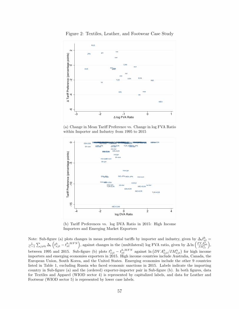
Figure 2: Textiles, Leather, and Footwear Case Study

AUS BRA

CAN

EUN

IDN

IND

JPN

MEX

RUS

TURUSA

aus bra

can

eun

idn

ind

jpn

mex

rus

tur

usa

-6-4

-20

2∆

Tarif

f Pre

fere

nce

(per

cent

age

poin

ts)

-3 -2 -1 0 1∆ log FVA Ratio

(a) Change in Mean Tariff Preference vs. Change in log FVA Ratiowithin Importer and Industry from 1995 to 2015

BRA-AUSCHN-AUS

IDN-AUS

IND-AUS MEX-AUSTUR-AUSTWN-AUS BRA-CANCHN-CANIDN-CAN IND-CAN

MEX-CAN

TUR-CANTWN-CAN BRA-EUNCHN-EUN

IDN-EUNIND-EUN

MEX-EUNTUR-EUN

TWN-EUN

BRA-JPNCHN-JPN

IDN-JPN IND-JPN MEX-JPN

TUR-JPN

TWN-JPN BRA-KOR

CHN-KOR

IDN-KORIND-KOR

MEX-KOR

TUR-KOR

TWN-KORBRA-USACHN-USAIDN-USA IND-USA

MEX-USA

TUR-USATWN-USA bra-auschn-aus

idn-aus

ind-aus mex-austur-austwn-aus bra-canchn-canidn-can ind-can

mex-can

tur-cantwn-can bra-eunchn-eun

idn-eunind-eun

mex-euntur-eun

twn-eun bra-jpnchn-jpn

idn-jpn

ind-jpn

mex-jpn

tur-jpntwn-jpn bra-kor

chn-kor

idn-korind-kor

mex-kor

tur-kor

twn-kor

bra-usa

chn-usa

idn-usa ind-usa

mex-usa

tur-usa

twn-usa

-15

-10

-50

Tarif

f Pre

fere

nce

(per

cent

age

poin

ts)

-4 -2 0 2 4log DVA Ratio

(b) Tariff Preferences vs. log DVA Ratio in 2015: High IncomeImporters and Emerging Market Exporters

Note: Sub-figure (a) plots changes in mean preferential tariffs by importer and industry, given by ∆tthxt =

1C−1

∑j 6=h ∆t

(thxjt − t

h,MFNxt

), against changes in the (multilateral) log FVA ratio, given by ∆ ln

(FV Ah

xt

IMhxt

),

between 1995 and 2015. Sub-figure (b) plots thxjt − th,MFNxt against ln

(DV Ahxjt/IM

hxjt

)for high income

importers and emerging economies exporters in 2015. High income countries include Australia, Canada, theEuropean Union, South Korea, and the United States. Emerging economies include the other 9 countrieslisted in Table 1, excluding Russia who faced economic sanctions in 2015. Labels indicate the importingcountry in Sub-figure (a) and the (ordered) exporter-importer pair in Sub-figure (b). In both figures, datafor Textiles and Apparel (WIOD sector 4) is represented by capitalized labels, and data for Leather andFootwear (WIOD sector 5) is represented by lower case labels.

57

A Theory Appendix

A.1 Proof of Proposition 1

To prove Proposition 1 we need to derive the necessary and sufficient conditions under which:(i) dτo

dνfh< 0 and (ii) dτo

dνhf< 0. These derived expressions will be Conditions 1 and 2 in the

text.Recall that τ o is given by the first order condition of Home’s indirect utility function

with respect to the tariff:Vτ (τ

o) = 0, (A1)

where Vτ ≡ dV h

dτ= ∂V (ph,Ih)

∂phdph

dτ+ ∂V (ph,Ih)

∂IhdIh

dτ, using dIh

dτ= ∂I(ph,pf )

∂phdph

dτ+ ∂I(ph,pf )

∂pfdpf

dτ. Taking

the total derivative of (A1) characterizes the relationship between the optimal tariff andGVC inputs in DVA (νfh) and FVA (νhf ):

Vττdτo + Vτνfh

dνfh + Vτνhf dνhf = 0, (A2)

where we again use subscripts as shorthand for derivatives: Vττ ≡ d2V h

dτ2, Vτνfh

≡ d2V h

dτdνfhand

Vτνhf ≡d2V h

dτdνhf.

Consider part (i) of Proposition 1 first, focusing on the DV A input, νfh and holding νhffixed. Evaluating (A2) at the optimal tariff, we have:

dτ o

dνfh= −

VτνfhVττ

∣∣∣∣τo. (A3)

By the second order condition of the optimal tariff problem, Vττ∣∣τo< 0. Thus, the necessary

and sufficient condition for the optimal tariff to be declining in DVA-inputs reduces to:

dτ o

dνfh< 0 ⇐⇒ Vτνfh

∣∣∣τo< 0. (A4)

Using the first order condition in (2.16), together with expressions (2.17) and (2.18), collect-ing terms, using the market clearing condition, and applying the envelope condition at τ o,

58

we have:

Vτνfh

∣∣∣τo

=d

dνfh

(dV

dτ

)(A5)

=d

dνfh

(VI

(τ o − 1)pf

dMx

dτ−Mx

dpf

dτ−drhfdph

νhfdph

dτ+drfhdpf

νfhdpf

dτ

)(A6)

=d

dνfh

(VIdpf

dτ

(τ o − 1)Ef

x (εfx − 1)−drhfdph

νhf1

λ+drfhdpf

νfh︸ ︷︷ ︸=0@τo

)(A7)

= VI+

dpf

dτ-

d

dνfh

((τ o − 1)Ef

x (εfx − 1)−drhfdph

νhf1

λ+drfhdpf

νfh

)∣∣∣∣∣τ=τo

. (A8)

From here, we can rewrite (A4) as:

dτ o

dνfh< 0 ⇐⇒ d

dνfh

((τ o − 1)Ef

x (εfx − 1)−drhfdph

νhf1

λ+drfhdpf

νfh

)∣∣∣∣∣τo

> 0 (A9)

Rewriting the second inequality delivers the necessary and sufficient condition for the optimaltariff to be decreasing in the quantity of Home’s value added used in foreign production statedin Condition 1:1[

drfhdpf

+d

dνfh

(drfhdpf

)νfh +

d

dνfh

(drhfdph

1

|λ|

)νhf +

d

dνfh

((τ o − 1)Ef

x (εfx − 1)

)]∣∣∣∣∣τo

> 0.

The indirect effects of a change in νfh on Home’s terms-of-trade motive and on pass-throughrates (from tariffs to prices, embedded in λ, and from final goods prices to GVC income in

thedrcjdpc

terms) are generally ambiguous in sign. As long as these indirect effects are not bothnegative and large, Condition 1 will be satisfied, and Home’s optimal tariff will be decreasingin its domestic GVC inputs embodied in Foreign production.

The derivation of the necessary and sufficient condition for FV A closely parallels thatabove, so we do not repeat it here; the result is Condition 2 in the text.

A.2 A Functional Form Example

This appendix presents a simple functional-form version of the model with quadratic utilityand Cobb-Douglass production for the non-numeraire good. This exercise fixes ideas andallows us to derive the explicit form of the optimal tariff in terms of model primitives.

1The derivative d

dνfh

includes the direct influence of νfh as well as any potential changes in final good

prices. For economy of notation, we subsume these partial effects in the total derivative; e.g. d

dνfh

(drfhdpf

)=

∂2rfh(pf ,~νf )

∂pf∂νfh

+∂2rfh(p

f ,~νf )

∂pf 2dpf

dνfh

.

59

A.2.1 Set-up

The structure of the model follows the set up described in Section 2.1, with identical notationand assumptions except where noted below.

Functional Form Assumption 1. Preferences are described by the following utility func-tion:

U(dcy, dcx) = αdcy + βcdcx −

1

2dcx

2 (A10)

for c ∈ h, f, where α, βc > 0 are exogenous parameters.

Functional Form Assumption 2. Technology is given by the production functions:

qcx = (2γlcxVc)

12 qcy = lcy (A11)

for c ∈ h, f, where γ > 0 is an exogenous technology parameter and V c = νch+νcf representsthe total composite value added used in production of good x in country c ∈ h, f.

The next assumption defines the division of quasi-rents between locally- and foreign-sourced value added inputs.

Functional Form Assumption 3. Let rch = rcf ≡ rc for c ∈ h, f; i.e. the (pre-tax)per-unit price paid to value added-inputs is the same for domestically- and foreign-sourcedinputs.

This assumption is a sensible benchmark in our setting where Home and Foreign GVCinputs are perfect substitutes in production.2

The final assumption ensures that x is Home’s natural import good – or equivalently,Foreign has a (preference-derived) comparative advantage in production of good x:

Functional Form Assumption 4. Let βh > βf and V h = V f ≡ V .

Focusing on demand-side drivers of trade simplifies the derivation of the closed-formtariff expression. It also serves a valuable expositional role in our later comparative staticsexercises. In our later comparative statics, we will hold the total level of composite valueadded input (V ) fixed in each country while varying the composition of GVC inputs usedin production across sources; this approach allows us to clearly identify the direct, first-order influence of GVC production linkages on optimal tariff setting apart from potentialsecond-order effects via generic disruptions in production and trade volumes.

A.2.2 Solution

Production. Together, profit maximization and labor market clearing determine the sup-ply functions for each good in each country c ∈ h, f:

qcx(pc) = γV pc qy(p

c) = Lc − 1

2γV pc2. (A12)

2As noted earlier, in specific factors settings, the division of quasi-rents among multiple specific factorsis generally indeterminate. Our key results obtain under alternative rent-sharing assumptions as long as thepass-through rate from local prices to GVC-inputs is strictly positive.

60

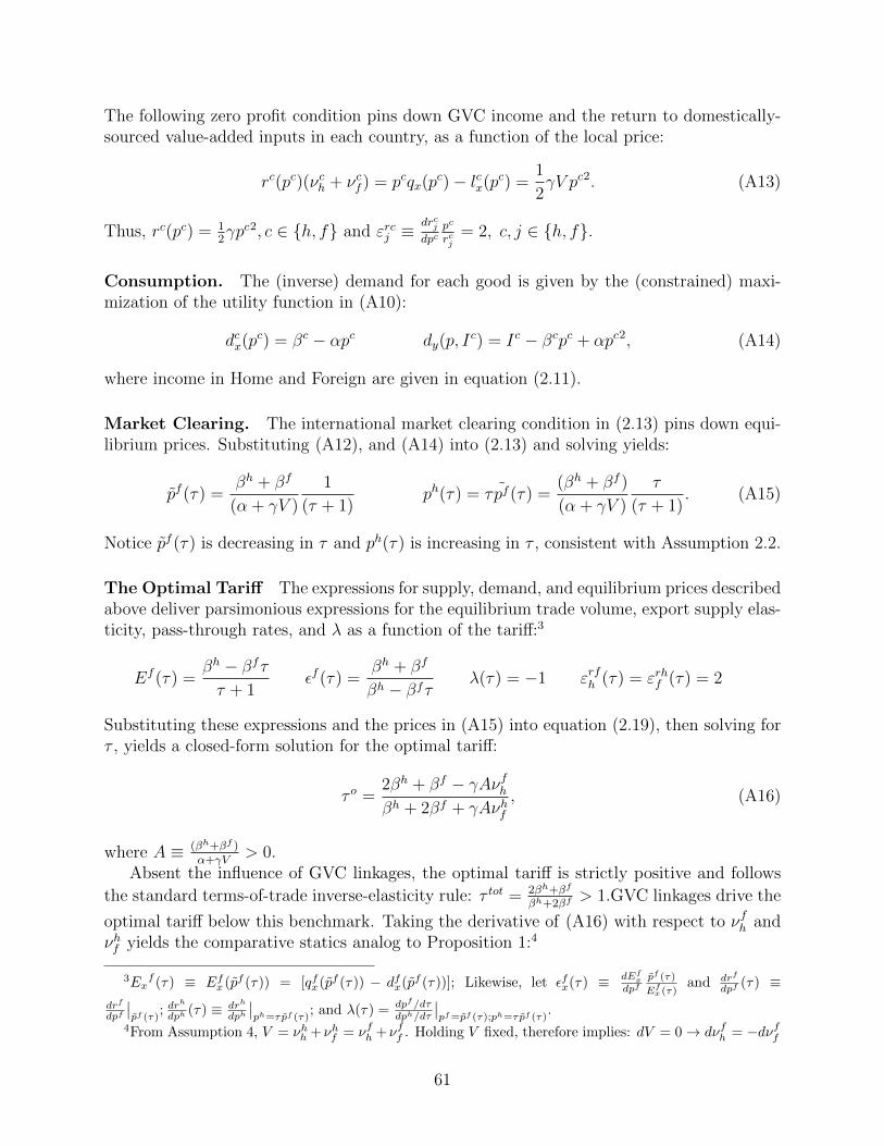
The following zero profit condition pins down GVC income and the return to domestically-sourced value-added inputs in each country, as a function of the local price:

rc(pc)(νch + νcf ) = pcqx(pc)− lcx(pc) =

1

2γV pc2. (A13)

Thus, rc(pc) = 12γpc2, c ∈ h, f and εrcj ≡

drcjdpc

pc

rcj= 2, c, j ∈ h, f.

Consumption. The (inverse) demand for each good is given by the (constrained) maxi-mization of the utility function in (A10):

dcx(pc) = βc − αpc dy(p, I

c) = Ic − βcpc + αpc2, (A14)

where income in Home and Foreign are given in equation (2.11).

Market Clearing. The international market clearing condition in (2.13) pins down equi-librium prices. Substituting (A12), and (A14) into (2.13) and solving yields:

pf (τ) =βh + βf

(α + γV )

1

(τ + 1)ph(τ) = τ pf (τ) =

(βh + βf )

(α + γV )

τ

(τ + 1). (A15)

Notice pf (τ) is decreasing in τ and ph(τ) is increasing in τ , consistent with Assumption 2.2.

The Optimal Tariff The expressions for supply, demand, and equilibrium prices describedabove deliver parsimonious expressions for the equilibrium trade volume, export supply elas-ticity, pass-through rates, and λ as a function of the tariff:3

Ef (τ) =βh − βfττ + 1

εf (τ) =βh + βf

βh − βfτλ(τ) = −1 εrfh (τ) = εrhf (τ) = 2

Substituting these expressions and the prices in (A15) into equation (2.19), then solving forτ , yields a closed-form solution for the optimal tariff:

τ o =2βh + βf − γAνfhβh + 2βf + γAνhf

, (A16)

where A ≡ (βh+βf )α+γV

> 0.Absent the influence of GVC linkages, the optimal tariff is strictly positive and follows

the standard terms-of-trade inverse-elasticity rule: τ tot = 2βh+βf

βh+2βf> 1.GVC linkages drive the

optimal tariff below this benchmark. Taking the derivative of (A16) with respect to νfh andνhf yields the comparative statics analog to Proposition 1:4

3Exf (τ) ≡ Efx (pf (τ)) = [qfx(pf (τ)) − dfx(pf (τ))]; Likewise, let εfx(τ) ≡ dEf

x

dpfpf (τ)

Efx(τ)

and drf

dpf(τ) ≡

drf

dpf

∣∣pf (τ)

; drh

dph(τ) ≡ drh

dph

∣∣ph=τpf (τ)

; and λ(τ) = dpf/dτdph/dτ

∣∣pf=pf (τ);ph=τpf (τ)

.4From Assumption 4, V = νhh +νhf = νfh +νff . Holding V fixed, therefore implies: dV = 0→ dνfh = −dνff

61

Lemma 1. Subject to Functional Form Assumptions 1-4, Home’s optimal tariff is decreasingin the share of GVC-inputs used in production:

dτ o

dνhf

∣∣∣∣∣dV=0

< 0 anddτ o

dνfh

∣∣∣∣∣dV=0

< 0.

Proof. With dV = 0,

dτ o

dνhf= − γAνfhτ

o

βh + 2βf + γAνhf< 0

dτ o

dνfh= − γAνfh

βh + 2βf + γAνhf< 0.

A.3 The Optimal Tariff with Endogenous GVCs

This appendix generalizes the model to allow for endogenous changes in the use of value-added inputs across sectors and countries in response to price changes. As noted in themain text, we allow frictions to limit the substitutability of inputs across end-use sectors ordestinations, so that the equilibrium returns to inputs may differ non-systematically acrosscountries. We assume only that (i) the return to, and the use of, the value-added inputs areweakly increasing in the local price of the final good that they are used to produce, and (ii)the vector of final goods prices uniquely pins down the global distribution and returns tovalue-added inputs.

Assumption A.1. Let:

1. rcj = rcj(pc, ~νc(~p)) ≡ rcj(~p) where

∂rcj (ph,pf )

∂pc≥ 0 for c, j ∈ h, f,

2. νcj = νcj (~r(~p)) ≡ νcj (~p) where∂νcj (ph,pf )

∂pc≥ 0 for c, j ∈ h, f,

To streamline analysis, we adopt quasi-linear preferences, which removes potential incomeeffects that otherwise complicate exposition:

U c = dc0 + ux(dcx), c ∈ x, y. (A17)

As before, national income is given by:

Ih = qy + phqhx(ph, ~ν) + (ph − pf )Mx(ph, ~ν) + rfh(~p)νfh(~p)︸ ︷︷ ︸

≡DV Ah(~p)

− rhf (~p)νhf (~p)︸ ︷︷ ︸≡FV Ah(~p)

. (A18)

The Home government chooses its optimal tariff to maximize aggregate indirect utility, sub-ject to the arbitrage and market clearing conditions in (2.12)-(2.13), which together pin downthe equilibrium prices pf and ph = τ pf as a function of the tariff.

The first order condition of the optimal tariff problem is largely unchanged from (2.16),with one important exception. Now, since the pattern of value-added use depends on prices,

and dνhf = −dνhh . Under the functional forms adopted in this example, neither νhh nor νff enter the optimaltariff expression (i.e. demand and supply for good x are independent of the composition of input sourcing),so the results in Lemma 1 are immediate.

62

any change in the tariff may disrupt the pattern of production and trade through ~ν in additionto the typical price mechanism (holding ~ν fixed). Using Roy’s identity and collecting terms,the first order condition may be written:

Vτ = VI

[(τ o − 1)pf

dMx

dτ−Mx

dpf

dτ+ ph∇~ν qhx ·Dτ~ν −

dFV Ah

dτ+dDV Ahdτ

]= 0, (A19)

where we use ∇~νqhx to denote the (partial) gradient of qhx(ph, ~ν) with respect to the value-added inputs in ~ν and Dτ~ν for the derivative of ~ν with respect to the tariff.5

The first two terms in brackets reflect the terms-of-trade motive, while the third termcaptures any change in Home’s production of the final good as a result of the endogenouschange in the pattern of value-added input use. The last two terms capture the effect ofa change in the tariff on GVC income via FV A and DV A. Applying the market clearingcondition (Mx = Ef

x ), decomposing the change in trade volume into the local-price effectversus “GVC relocation effect”,6 expanding the DV A and FV A terms, and rearrangingyields:(

(τ o − 1)εfx − 1)Efx

dpf

dτ− pf∇~νEf

x ·Dτ~ν +∇DV Ah ·Dτ~p︸ ︷︷ ︸≡ dDV Ah

dτ

−∇FV Ah ·Dτ~p︸ ︷︷ ︸≡ dFV Ah

dτ

= 0, (A20)

where εfx = ∂Efx (pf ,~ν)∂pf

pf

Efxis foreign export supply (price) elasticity, ∇DV Ah and ∇FV Ah

represent the gradients of each GVC income term with respect to the world price vector,

and Dτ~p = (dph

dτ, dp

f

dτ) is the derivative of the price vector with respect to the tariff. Dividing

through by the trade volume and dpf

dτyields:

(τ o − 1)εfx = 1 +∇FV Ah · ~Λ

Efx

− ∇DV Ah ·~Λ

Efx

+ η, (A21)

where ~Λ ≡ Dτ ~pdpf/dτ

=(

1λ, 1)

and we use η ≡ pf

Efx∇~νEf

x∂~ν∂~p

Λᵀ to capture the change in final goods

trade as a result of the endogenous change in input use.Decomposing the GVC terms into pass-though elasticities and GVC income, we can write:

∇FV Ah · ~ΛEfx

=1

Efx

(νhf∇rhf + rhf∇νhf

)· ~Λ =

(rhfν

hf

phEfx

)(ph

rhf∇rhf · ~Λ︸ ︷︷ ︸≡−εrhf

+ph

νhf∇νhf · ~Λ︸ ︷︷ ︸≡−ενhf

)(A22)

5In terms of notation, we use ∇b to represent the (complete) (1× 2) gradient of b(~p) with respect to theworld price vector ~p = (ph, pf ); ∇~νa to represent the (partial) (1 × 4) gradient of a(p, ~ν) with respect to

~ν ≡ (νhh , νhf , ν

ff , ν

fh); and ∂~ν

∂~p for the (4× 2) Jacobian of ~ν(~p). Thus, ∇~ν qhx ·Dτ~ν = ∇~ν qhx ∂~ν∂~p ·Dτ~p.

6 dMx

dτ =dEf

x

dτ =∂Ef

x(pf ,~ν)

∂pfdpf

dτ +∇~ν Efx ·Dτ~ν, where ∇~νEfx is the (partial) gradient of Efx (pf , ~ν) with respect

to the arguments in vector ~ν. Since there are no income effects, ∇~νEfx ·Dτ~ν = −∇~νqhx ·Dτ~ν.

63

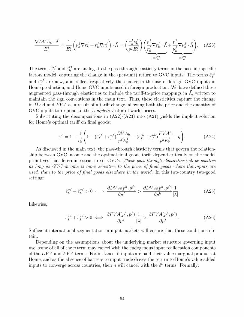
∇DV Ah · ~ΛEfx

=1

Efx

(νfh∇r

fh + rfh∇ν

fh

)· ~Λ =

(rfhν

fh

pfEfx

)(pf

rfh∇rfh · ~Λ︸ ︷︷ ︸≡εrfh

+pf

νfh∇νfh · ~Λ︸ ︷︷ ︸≡ενfh

). (A23)

The terms εrhf and εrfh are analogs to the pass-through elasticity terms in the baseline specific

factors model, capturing the change in the (per-unit) return to GVC inputs. The terms ενhfand ενfh are new, and reflect respectively the change in the use of foreign GVC inputs inHome production, and Home GVC inputs used in foreign production. We have defined theseaugmented pass-through elasticities to include the tariff-to-price mappings in ~Λ, written tomaintain the sign conventions in the main text. Thus, these elasticities capture the changein DV A and FV A as a result of a tariff change, allowing both the price and the quantity ofGVC inputs to respond to the complete vector of world prices.

Substituting the decompositions in (A22)-(A23) into (A21) yields the implicit solutionfor Home’s optimal tariff on final goods:

τ o = 1 +1

εfx

(1− (εrfh + ενfh )

DV Ah

pfEfx

− (εrhf + ενhf )FV Ah

phEfx

+ η

). (A24)

As discussed in the main text, the pass-through elasticity terms that govern the relation-ship between GVC income and the optimal final goods tariff depend critically on the modelprimitives that determine structure of GVCs. These pass-through elasticities will be positiveas long as GVC income is more sensitive to the price of final goods where the inputs areused, than to the price of final goods elsewhere in the world. In this two-country two-goodsetting:

ενfh + ενfh > 0 ⇐⇒ ∂DV A(ph, pf )

∂pf>∂DV A(ph, pf )

∂ph1

|λ|(A25)

Likewise,

ενhf + ενhf > 0 ⇐⇒ ∂FV A(ph, pf )

∂ph1

|λ|>∂FV A(ph, pf )

∂pf. (A26)

Sufficient international segmentation in input markets will ensure that these conditions ob-tain.

Depending on the assumptions about the underlying market structure governing inputuse, some of all of the η term may cancel with the endogenous input reallocation componentsof the DV A and FV A terms. For instance, if inputs are paid their value marginal product atHome, and as the absence of barriers to input trade drives the return to Home’s value-addedinputs to converge across countries, then η will cancel with the εν terms. Formally:

64

Lemma 2. If rhf = ph ∂qhx

∂νhfand rhh = ph ∂q

hx

∂νhh, then as rhh → rfh and if dνfh → −dνhh , then:

τ o → 1 +1

εfx

(1− εrfh

DV Ah

pfEfx

− εrhfFV Ah

phEfx

),

where εfx ≡[∂Efx (pf ,~ν)

∂pf+∇~ν Ef

x ·(Dpf~ν+Dph~ν

1λ

)]pf

Efxis the elasticity of export supply allowing

for endogenous changes in value-added input use across countries.

Proof. Substituting the conditions rhf = ph ∂qhx

∂νhfand rfh = rhh = ph ∂q

hx

∂νhhand dνfh = −dνhh into

the first order condition in (A19), cancelling terms, and solving yields the result.

A.4 Endogenous Input Tariffs with Endogenous GVCs

We now introduce input tariffs to the general equilibrium model with endogenous GVCs. Themodel and assumptions are as described in Appendix A.3, with one change. We now permitthe home country to levy an ad-valorem tax on foreign-sourced inputs used in domesticproduction: g ∈ [0, 1], applied to the local price of imported inputs, rhf , so that trade taxrevenue is now:

Rh = (ph − pf )Mhx + gFV Ahs . (A27)

National income is given by:

Ih = qy + phqhx(ph, ~ν) + (ph − pf )Mx(ph, ~ν) + rfh(~p)νfh(~p)︸ ︷︷ ︸

≡DV Ah(~p)

−(1− g) rhf (~p)νhf (~p)︸ ︷︷ ︸≡FV Ah(~p)

. (A28)

The Home government (again) chooses its optimal tariffs to maximize aggregate indirectutility, subject to the arbitrage and market clearing conditions in (2.12)-(2.13).

The Optimal Tariff on Final Goods Given any arbitrary input tariff g, the optimaltariff on final goods is described implicitly by the first order condition:

Vτ = VI

[(τ o − 1)pf

dMx

dτ−Mx

dpf

dτ+ ph∇~ν qhx ·Dτ~ν−(1−g)

dFV Ah

dτ+dDV Ahdτ

]= 0. (A29)

The only difference between this expression and that in (A19) is the introduction of thecoefficient (1− g) on the FV A term. Consistent with the discussion in Section 2.5, this newterm reflects the fact that an input tariff allows the Home government to recapture someof the protectionist rents associated with its final goods tariff that would otherwise flow toforeign-owned GVC inputs. Following the same solution methodology in Appendix A.3, itis straightforward to show the the optimal final goods tariff in the presence of an arbitraryinput tax on foreign-sourced value-added inputs is given by:

τ o = 1 +1

εfx

(1− (εrfh + ενfh )

DV Ah

pfEfx

− (1− g)(εrhf + ενhf )FV Ah

phEfx

+ η

). (A30)

65

The Optimal Input Tariff The optimal input tariff is defined implicitly by the followingfirst order condition:

Vg=VI

[(τ−1)pf

dMx

dg−Mx

dpf

dg+ph∇~νqhx ·Dg~ν+

dDV Ahdg

−(1−go)dFV Ah

dg+FV A

]=0. (A31)

Applying the market clearing condition and reorganizing terms, we then have:

(go−1)[rhfdνhfdg

+νhfdrhfdg

]︸ ︷︷ ︸

≡ dFV Ahdg

−rhfνhf−ph∇~νqhx ·Dg~ν= (τ−1)pfEfx

dg−Ef

x

dpf

dg+∇DV Ah ·Dg~p︸ ︷︷ ︸

≡ dDV Ahdg

,

If value-added inputs used in Home production are paid their value marginal product, so

that rhj = ph ∂qhx(ph,~ν)

∂νhj, j ∈ h, f, we can further simplify this first order condition to:

(goξhf − 1

)drh∗fdg

νhf = (τ−1)pfEfx

dg−Ef

x

dpf

dg+∇DV Ah ·Dg~p+ rhh

dνhhdg

, (A32)

where rh∗f ≡ (1 − g)rhf and ξhf ≡rhfνhf∇~rνhf · Dg~r

1drhf /dg

is the elasticity of foreign GVC inputs

used in Home production with respect to the change in the rates of return paid to ForeignGVC inputs. From here, we make two observations. First, the optimal input tariff (like theoptimal final goods tariff) follows an own inverse elasticity rule, moderated by GVC cross-linkages (how final goods trade, and therefore tariff revenue associated with final goods trade,changes with g; how DV A responds to g, and how the return to home’s domestically-usedvalue-added inputs (νhh) changes with g). Second, the behavior and sign of these cross-effectswill depend on model primitives, including whether home and foreign value-added inputs arecomplements or substitutes in production of final goods and whether the induced reallocation

of GVC inputs makes global production of final goods more or less efficient (so that dpf

dgQ 0).

As a final point, note that if both the optimal tariff on final goods and the optimal inputtariff are characterized by interior solutions, they are described by the system of equationsin (A29) and (A31). In the resulting optimal tariff solutions, some (but not all) of the cross-effects in (A32) may be be eliminated envelope conditions if there are no other frictions toinput trade and input markets are perfectly competitive. Even so, general results are elusive,as Antras and Chor (2021) make clear in Section 6.3 of their recent Handbook chapter.Note that considerable caution must be exercised in this environment, since many standardmodelling assumptions about the nature of GVCs (including specific factors) lead to cornersolutions where the first order condition for input tariffs will not obtain.

A.5 Many-Country, Many-Good, Political Economy Model

This appendix derives the many-country many-good specific-factors version of the baselinemodel with political economy influences presented in Section 3.1 of the paper.

66

A.5.1 Set-up

Consider a many-country world in which a given home country, h, trades with C tradingpartners. Define the of countries by C = 0, 1, ..., C. There are S + 1 final goods. Thenumeraire is indexed by 0; all other (non-numeraire) final goods are described by the setS = 1, ..., S. Final goods prices in each country c ∈ C are denoted by pcs, where s designatesthe final goods sector. The numeraire good is freely traded, so that pc0 = 1∀c ∈ C. We use~pc = (pc1, ..., p

cS) to denote the (1×S) vector of (non-numeraire) final goods prices in country

c, ~ps = (p0s, ..., p

Cs ) to denote the (1 × C + 1) vector of sector s prices in each country, and

~p = (~p0, ..., ~pC) to represent the complete (1× S(C + 1))vector of non-numeraire final goodsprices in every country world-wide.7

Preferences Each country is populated by a continuum of identical agents with identicalquasi-linear preferences, represented by the aggregate utility function:

U c(dc0,~dsc) = dc0 +

∑s≥1

us(dcs) ∀c ∈ C, (A33)

where dcs represents aggregate consumption of final good s in country c and sub-utilityover each non-numeraire good, us(·), is increasing, continuously differentiable, and strictlyconcave. We assume that every individual has sufficient income to consume a strictly positivequantity of the numeraire so that preferences over non-numeraire goods satisfy Gorman form.

Endowments Every country c ∈ C is endowed with a homogeneous factor, Lc,

Technology. Atomistic firms produce final goods in perfectly competitive markets. Tech-nology is summarized by the constant returns to scale production functions:

qcs = f cs (lcs, ν

csc, ~ν

cs∗) qc0 = lco (A34)

where qcs is the quantity of final good s produced in country c using lcs units of (homogeneous)labor, νcsc units of domestically-sourced value-added input, and a (1×C) vector of GVC inputssourced from from every country j 6= c ∈ C: ~νcs∗. As in the benchmark model, we proceedwithout specifying the the exact division of quasi-rents across the (many) value-added inputsused to make each final good; we assume only that the price paid to value-added input isincreasing in the local price of the final good that it is used to produce. Consistent withAssumption 2.1, we adopt:

Assumption A.2.

rcsj ≡ rcsj(pcs;~ν

cs) where

∂rcsj(pcs;~ν

cs)

∂pcs> 0 ∀c ∈ C, s ∈ S. (A35)

7It later proves useful to partition price vectors into domestic and foreign components [Bagwell andStaiger (1999)]. From the perspective of a given country h ∈ C, ~p ≡ (~ph, ~p∗), where ~p∗ is the (1×SC) vectorof prices in every country j 6= h ∈ C. Likewise, let ~ps ≡ (phs , ~p

∗s) where ~p∗s is the (1× C) vector of prices for

good s in every country other than country h.

67

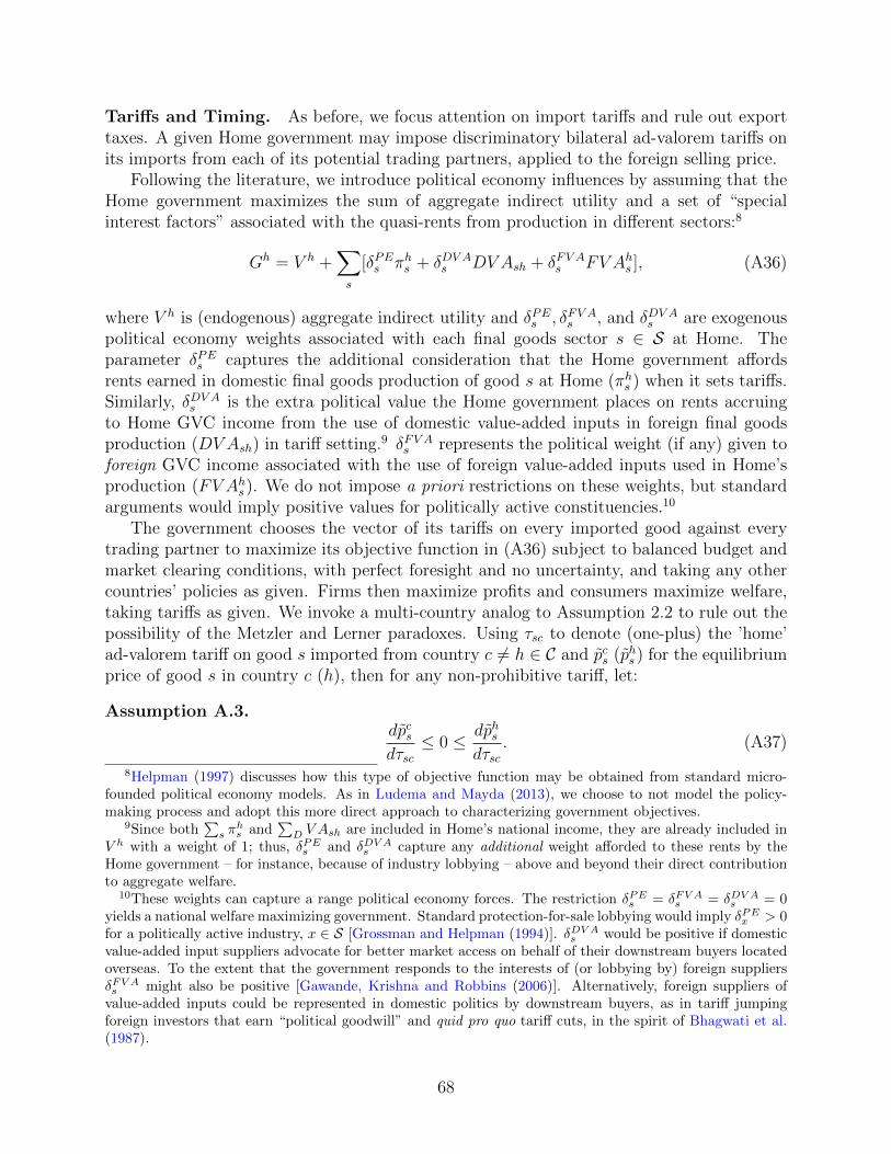
Tariffs and Timing. As before, we focus attention on import tariffs and rule out exporttaxes. A given Home government may impose discriminatory bilateral ad-valorem tariffs onits imports from each of its potential trading partners, applied to the foreign selling price.

Following the literature, we introduce political economy influences by assuming that theHome government maximizes the sum of aggregate indirect utility and a set of “specialinterest factors” associated with the quasi-rents from production in different sectors:8

Gh = V h +∑s

[δPEs πhs + δDV As DV Ash + δFV As FV Ahs ], (A36)

where V h is (endogenous) aggregate indirect utility and δPEs , δFV As , and δDV As are exogenouspolitical economy weights associated with each final goods sector s ∈ S at Home. Theparameter δPEs captures the additional consideration that the Home government affordsrents earned in domestic final goods production of good s at Home (πhs ) when it sets tariffs.Similarly, δDV As is the extra political value the Home government places on rents accruingto Home GVC income from the use of domestic value-added inputs in foreign final goodsproduction (DV Ash) in tariff setting.9 δFV As represents the political weight (if any) given toforeign GVC income associated with the use of foreign value-added inputs used in Home’sproduction (FV Ahs ). We do not impose a priori restrictions on these weights, but standardarguments would imply positive values for politically active constituencies.10

The government chooses the vector of its tariffs on every imported good against everytrading partner to maximize its objective function in (A36) subject to balanced budget andmarket clearing conditions, with perfect foresight and no uncertainty, and taking any othercountries’ policies as given. Firms then maximize profits and consumers maximize welfare,taking tariffs as given. We invoke a multi-country analog to Assumption 2.2 to rule out thepossibility of the Metzler and Lerner paradoxes. Using τsc to denote (one-plus) the ’home’ad-valorem tariff on good s imported from country c 6= h ∈ C and pcs (phs ) for the equilibriumprice of good s in country c (h), then for any non-prohibitive tariff, let:

Assumption A.3.dpcsdτsc≤ 0 ≤ dphs

dτsc. (A37)

8Helpman (1997) discusses how this type of objective function may be obtained from standard micro-founded political economy models. As in Ludema and Mayda (2013), we choose to not model the policy-making process and adopt this more direct approach to characterizing government objectives.

9Since both∑s π

hs and

∑D V Ash are included in Home’s national income, they are already included in

V h with a weight of 1; thus, δPEs and δDVAs capture any additional weight afforded to these rents by theHome government – for instance, because of industry lobbying – above and beyond their direct contributionto aggregate welfare.

10These weights can capture a range political economy forces. The restriction δPEs = δFV As = δDVAs = 0yields a national welfare maximizing government. Standard protection-for-sale lobbying would imply δPEx > 0for a politically active industry, x ∈ S [Grossman and Helpman (1994)]. δDVAs would be positive if domesticvalue-added input suppliers advocate for better market access on behalf of their downstream buyers locatedoverseas. To the extent that the government responds to the interests of (or lobbying by) foreign suppliersδFV As might also be positive [Gawande, Krishna and Robbins (2006)]. Alternatively, foreign suppliers ofvalue-added inputs could be represented in domestic politics by downstream buyers, as in tariff jumpingforeign investors that earn “political goodwill” and quid pro quo tariff cuts, in the spirit of Bhagwati et al.(1987).

68

A.5.2 Solution

Production, consumption, and market clearing conditions are direct analogs to the two-by-two model presented in Section 2.1. The only substantive change is the additional simplifi-cation afforded by quasi-linear preferences: with sufficient income (as assumed), demand foreach non-numeraire good is independent of national income.11

Production In every country c ∈ C, profit maximization by atomistic firms and local labormarket clearing determine the supply function for each final good s ∈ S as a function oflocal final goods prices, taking value-added inputs and total labor endowment as given:

qcs(pcs;~ν

cs) = f cs (l

cs(p

cs), ν

csc, ~ν

cs∗) ∀s (A38)

qc0(~pc;~νc) = Lc −∑s

lcs(pcs;~ν

cs), (A39)

where lcs(pcs;~ν

cs) = arg maxlcs pcsf

cs (l

cs, ν

csc, ~ν

cs∗)− lcs ∀s ∈ S.

The zero profit condition in each sector s ∈ S implies that the total quasi-rent associatedwith production of good s in country c, πcs, is divided among the set of value-added inputsused to make the good:

πcs(pcs) = pcsq

cs(p

cs)− lcs(pcs) =

∑j∈C

rcsjνcsj. (A40)

where, by Assumption A.3 rcsj ≡ rcsj(pcs;~ν

cs) and

∂rcsj(pcs;~ν

cs)

∂pcs> 0 ∀s ∈ S and c, j ∈ C.

Consumption. With quasi-linear preferences, aggregate demand for non-numeraire goodsis independent of income. In every country c ∈ C:

dcs(pcs, I

c) ≡ dcs(pcs) = u′s

−1(pcs) ∀s ∈ S (A41)

dc0(~pc, Ic) = Ic −∑s

pcsdcs (A42)

V (~pc, Ic) = ζc(~pc) + Ic, (A43)

where V (~pc, Ic) is aggregate indirect utility and ζc ≡∑

s[us(dcs) − pcsd

cs] is total consumer

surplus in country c. National income (measured in the numeraire) is given by the totalvalue of final goods production at local prices, plus any tariff revenue, plus GVC incomefrom domestic value-added inputs used in foreign production (DV A), less any GVC incomepaid to foreign value-added inputs used in local production (FV A). For each country c ∈ C:

Ic = qc0 + ~pc · ~qc(~pc, ~νc) +Rc +∑s

∑j 6=c

rjsc(pjs;~ν

js)ν

jsc︸ ︷︷ ︸

≡DV Asc

−∑s

∑j 6=c

rcsj(pcs;~ν

cs)ν

csj︸ ︷︷ ︸

≡FV Acs

, (A44)

11Thus, dcs(pcs, I

c) ≡ dcs(pcs)∀s ∈ S, which simplifies foreign export supply elasticity which must otherwise

incorporate potential income effects via Foreign GVC income, as noted in footnote 16.

69

where tariff revenue is and Rc =∑

s

∑j 6=c(p

cs − pjs)M

csj(~ps;~νs) and M c

sj(·) is country c′simports of good s from country j.

Market Clearing. Prices are disciplined by a set of SC no-arbitrage conditions: phs ≤τhscp

cs,∀c 6= h ∈ C, s ∈ S.12 Equilibrium prices are then determined by the set of S market

clearing conditions that ensure global demand equals global supply for each non-numerairegood: ∑

c∈C

dcs(pcs) =

∑c∈C

qcs(pcs;~ν

cs) ∀ s ∈ S. (A45)

Balanced budget conditions for each country clear the market for the numeraire.

A.5.3 Politically-Motivated Bilateral Tariffs

Home’s politically optimal tariff schedule, ~τ o, maximizes its government objective functionin (A36) subject to market clearing conditions in (A45):

~τ o = arg max~τ

Gh ≡ V h +∑s

[δPEs πhs + δDV As DV Ash + δFV As FV Ahs ]

s.t. phs ≤ τhscpcs and pcs = pcs ∀ c 6= h ∈ C, s ∈ S

Home has SC first order conditions, one for every (non-numeraire) sector s ∈ S and tradingpartner c 6= h ∈ C. Notice that with quasi-linear preferences and a numeriare good, thereare no cross-price effects across sectors. For a given bilateral, sector-specific tariff applied toimports of good x from trading partner j, τhxj the first order condition implicitly defines theoptimal tariff:

Ghτhxj

= (τhxj − 1)pjxdMh

xj

dτhxj− Mh

xj

dpjxdτhxj

+ δPEx qhxdphxdτhxj

+ ΩRxj (A46)

+ (1 + δDV Ax )dDV Axhdτhxj

− (1− δFV Ax )dFV Ahxdτhxj

= 0. (A47)

The term ΩRxj captures the potential for trade diversion to change Home’s tariff revenue from

trade with countries other than j.13 Apart from this trade diversion term, extra notation,and the addition of political economy weights to the DV A and FV A terms, the only sub-stantive change from the first order condition in (2.16) is the introduction of the domesticpolitical economy term weighted by δPEs , which reflects well-understood “protection-for-sale”motivations in tariff setting [Grossman and Helpman (1994)].

In preparation for the empirical application, we now decompose the two GVC terms intopass-through elasticities and directly-observable measures of GVC income. Consider firstthe role of foreign value added embodied in domestic final goods (FV A). The bilateral tariff

12These bilateral arbitrage relationships hold with equality in the presence of trade: Mhsc > 0⇒ phs = τhscp

cs.

13For any s ∈ S, ΩRsj ≡∑c 6=j,h(τsc − 1)

[dpcsdτsj

Msc + pcsdMsc

dτsj

]. These trade diversion effects, which are

typical in multi-country trade models, are generally ambiguous absent and plausibly negligible (e.g. whentrade diversion is minimal; see Freund and Ornelas (2010)).

70

raises the local final goods price at Home (phx), which in turn increases the returns to foreignvalue-added inputs embodied in Home’s domestic production via rhxc(p

hx;~ν

hx). We decompose

this effect as follows:

dFV Ahxdτhxj

=∑c 6=h

[rhxcν

hxc

phx

(drhxcdphx

phxrhxc

)︸ ︷︷ ︸≡εrhxc≥0

]dphxdτhxj

= εrhx∗∑c 6=h

rhxcνhxc

phx

dphxdτhsj

= εrhx∗FV Ahxphx

dphxdτhxj

(A48)

The term εrhxc ≡drhxcdphx

phxrhxc

is the elasticity of foreign value-added input prices with respect tolocal final goods prices at Home. This elasticity is positive by Assumption A.3: a higherprice on a final good implies higher returns to the value-added used in its production. Inpreparation for the empirical application, we further assume that this elasticity is the sameacross all foreign input sources, so that εrhxc = εrhx∗ ∀c 6= h ∈ C (as reflected the second equalityabove).

Turning to the role of domestic value added in foreign final goods (DVA), the bilateraltariff alters foreign final goods prices, which feed back into the price of domestic value-addedinputs. We decompose the direct and indirect price effects of the tariff as follows:

dDV Axhdτhxj

=rjxhν

jxh

pjx

(drjxhdpjx

pjxrjxh

)︸ ︷︷ ︸≡εrjxh≥0

dpjxdτhxj

+∑c6=h,j

dDV Acxhdpcx

dpcxdτhxj︸ ︷︷ ︸

≡ΩDVAxj

= εrjxhDV Ajxhpjx

dpjxdτhxj︸ ︷︷ ︸

direct effect

+ΩDV Axj (A49)

The direct effect captures the impact of an increase in τhxj on the return to Home’s GVC inputsused by the country (j) on which the tariff is imposed. We collect any potential indirecteffects – how the Home’s tariff on country j might impact the return of Home’s GVC inputsused in third countries – in ΩDV A

xj .14 The strength of this direct effect is governed by the

elasticity εrjxh, which is positive by Assumption A.3: a higher price of good x in country jimplies a higher price for Home’s value-added inputs used in production of that good.

Substituting Equations (A48) and (A49) into the first order condition in (A47) andsolving yields the following expression for the politically-motivated bilateral tariff:

τhxj = 1 +1

εjxh

(1 +

δPEx qhx|λhxj|E

jxh

− (1 + δDV Ax )εrjxhDV AjxhpjxE

jxh

− (1− δFV Ax∗ )εrhx∗|λhxj|

FV AhxphxE

jxh

− Ωxj

). (A50)

Where λhxj ≡dpjxdτhxj

/ dphx

dτhxj< 0, Ej

xh is country j’s exports of x to Home, εjxh ≡dEjxhdpjx

pjxEjxh

> 0

represents bilateral, sector-specific export supply elasticity between country j and Home,

and Ωxj ≡ΩRxj+ΩDVAxj

(dpjx/dτhxj)E

jxh

captures any potential third-country effects of trade diversion.15

14ΩDVAxj ≡∑c6=h,j

dDV Acxh

dpcx

dpcxdτh

xj

=∑c6=h,j ε

rcxh

DV Acxh

pcx

dpcxdτh

xj

. As noted earlier, such third-country effects are

generally ambiguous and depend on trade diversion.15This bilateral tariff expression describes country i’s non-cooperative equilibrium response as a function

of all other countries’ tariff policies, which are implicitly captured in the trade volume, elasticity, price, andλ terms. Country i’s Nash equilibrium tariff is then given by (A50) evaluated at the world tariff vector for

71

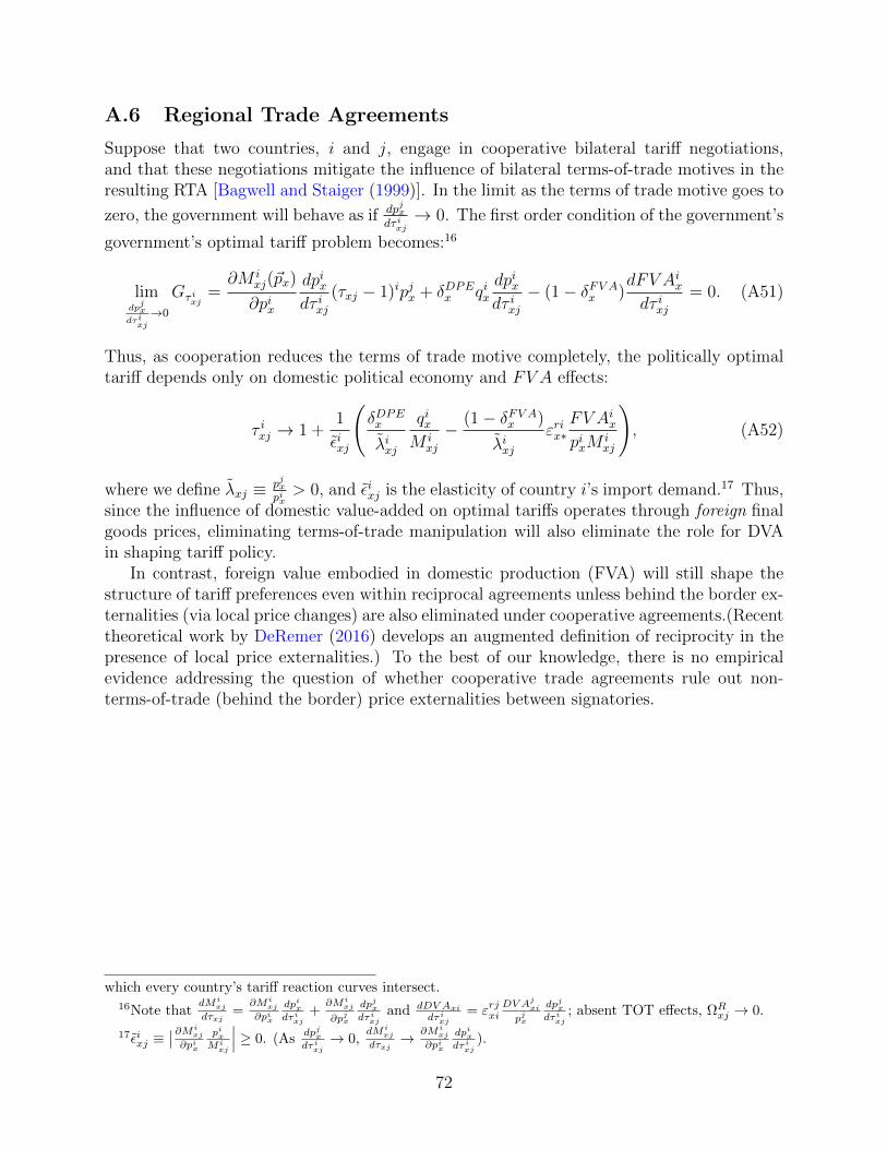
A.6 Regional Trade Agreements

Suppose that two countries, i and j, engage in cooperative bilateral tariff negotiations,and that these negotiations mitigate the influence of bilateral terms-of-trade motives in theresulting RTA [Bagwell and Staiger (1999)]. In the limit as the terms of trade motive goes to

zero, the government will behave as if dpjxdτ ixj→ 0. The first order condition of the government’s

government’s optimal tariff problem becomes:16

limdpjx

dτixj

→0

Gτ ixj=∂M i

xj(~px)

∂pix

dpixdτ ixj

(τxj − 1)ipjx + δDPEx qixdpixdτ ixj

− (1− δFV Ax )dFV Aixdτ ixj

= 0. (A51)

Thus, as cooperation reduces the terms of trade motive completely, the politically optimaltariff depends only on domestic political economy and FV A effects:

τ ixj → 1 +1

εixj

(δDPEx

λixj

qixM i

xj

− (1− δFV Ax )

λixjεrix∗

FV AixpixM

ixj

), (A52)

where we define λxj ≡ pjxpix> 0, and εixj is the elasticity of country i’s import demand.17 Thus,

since the influence of domestic value-added on optimal tariffs operates through foreign finalgoods prices, eliminating terms-of-trade manipulation will also eliminate the role for DVAin shaping tariff policy.

In contrast, foreign value embodied in domestic production (FVA) will still shape thestructure of tariff preferences even within reciprocal agreements unless behind the border ex-ternalities (via local price changes) are also eliminated under cooperative agreements.(Recenttheoretical work by DeRemer (2016) develops an augmented definition of reciprocity in thepresence of local price externalities.) To the best of our knowledge, there is no empiricalevidence addressing the question of whether cooperative trade agreements rule out non-terms-of-trade (behind the border) price externalities between signatories.

which every country’s tariff reaction curves intersect.16Note that

dMixj

dτxj=

∂Mixj

∂pix

dpixdτ i

xj+

∂Mixj

∂pjx

dpjxdτ i

xjand dDV Axi

dτ ixj

= εrjxiDV Aj

xi

pjx

dpjxdτ i

xj; absent TOT effects, ΩRxj → 0.

17εixj ≡∣∣∂Mi

xj

∂pix

pixMi

xj

∣∣∣ ≥ 0. (Asdpjxdτ i

xj→ 0,

dMixj

dτxj→ ∂Mi

xj

∂pix

dpixdτ i

xj).

72

B Empirical Appendix

This appendix presents details regarding the data we use and collects supplemental empiricalresults.

B.1 Data Details

B.1.1 Value-Added Content

Our measures of domestic content in foreign production and foreign content in domesticproduction can be motivated as an application of the ‘global value chain income’ decompo-sition of final goods developed in Los, Timmer and de Vries (2015). Intuitively, the globalinput-output table enables one to trace backwards through the production process to assessthe value and identify the national origin of the intermediate inputs used (both directlyand indirectly) to produce each country’s final goods. With this information, one can (forexample) compute the amount of Canadian value added embodied in US-produced autos.We briefly describe the computation here.

Let i, j ∈ 1, 2, . . . , C denote countries and s ∈ 1, 2, . . . , S denote industries. TheWorld Input-Output Database includes an input shipments matrix, IIt, with (S×S) dimen-sional block elements IIijt(s, s

′) that record input shipments from sector s in country i tosector s′ in country j. These matrices can easily be re-written in share form. Let Aijt be a(S × S) dimensional matrix with elements Aijt(s, s

′) = IIijt(s, s′)/Yj(s

′), which record theshare of inputs from sector s in country i used by sector s′ in country j as a share of grossoutput in sector s′ in country j. Then assemble blocks Aijt into the global input-outputmatrix At. The Leontief inverse of the global input-output matrix, [I − At]

−1, times any(SC×1) vector of final goods output equals yields the (SC×1) vector of gross output (fromall countries and industries) required to produce those final goods.

Let fit be the (S × 1) vector of final goods produced in country i, which are directlyreported in the World Input-Output Database. Stack these into a (SC × 1) vector ft,and compute Yt ≡ [I − At]−1diag(ft). Breaking this down, Yt contains block elements Yijtwhich are S × S matrices describing output from country i used (directly or indirectly) toproduce final goods in country j. Each sub-component Yijt(s, s

′) is the amount of outputfrom industry s in country i used in producing final output in industry s′ in country j.

These output requirements can be translated into value-added content requirements ifwe know the value added to output ratios in each sector s and source country i: Rit(s).The total amount of value added from country i embodied in country j’s production in aparticular industry x ∈ S is: V Ajxit ≡

∑sRit(s)Yijt(s, x). We use these value added elements

to construct proxies for country i’s domestic value added embodied in foreign productionof each sector s ∈ S in trading partner j 6= i ∈ C (DV Ajsit) and foreign value addedembodied in country i’s domestic production of s (FV Aist). Specifically, for a given good x,DV Ajxit ≡ V Ajxit and FV Aixt ≡

∑c 6=i∈C V A

ixct.

We obtain data to implement these calculations from the World Input-Output Database.The data is available at http://www.wiod.org and documented in Dietzenbacher et al.(2013) and Timmer et al. (2015). One complication in using these data is that there are twovintages of the database. The WIOD Release 2013 database contains an annual sequence

73

of global input-output tables for the 1995-2011 period covering 35 industries across 27 EUcountries and 13 other major countries.18 We augment this base data set using the WIODRelease 2016 data, which covers 2000-2014 period.

Because the Release 2013 and Release 2016 data are not fully compatible in terms ofunderlying definitions and data sources, they do not agree exactly in overlapping years. Wecompute value-added contents using the Release 2013 data, and treat these as the baselinedata for 1995-2010. We then also separately compute value-added contents for 2010-2014using the using data from Release 2016. Using growth rates from this Release 2016 data, wethen extrapolate levels from the Release 2013 data forward in time. In executing this linkageprocedure, we also map Release 2016 industries into Revision 2013. While Release 2016 hasslightly more disaggregated data than Release 2013, such that the sector mapping is manyto one in almost all cases, there is one case where it is not. In Release 2016, the Textilesand Leather and Footwear sectors are pooled together, while they are reported separately inRelease 2013. We thus apply growth rates for the pooled sector to extrapolate forward thetwo individual sectors in the Release 2013 data.

A second technical issue concerns the EU. In both data sets, EU members are reportedas individual countries. We compute value added content using the fully disaggregatedcountry data, and then we aggregate value-added contents across EU countries to form theEU composite in our data.

B.1.2 Tariffs

As noted in Section 3.5, we draw our data from UNCTAD (TRAINS) and the WTO viathe WITS website [http://wits.worldbank.org]. Multilateral MFN applied tariffs aretypically available in the WTO data, while bilateral applied tariffs are from TRAINS. Wefaced a number of challenges in transforming these raw data sources into a consistent set oftariff measures. Below we describe our procedure to clean and aggregate the tariff data.

First, there are a handful of instances in which a country’s entire bilateral tariff scheduleis missing in one of our four benchmark years. In most of these cases, when we can beconfident that there were no major trade policy changes in that year, we take the tariffschedule from the closest available year for that country. In a few instances, we insteadexclude the importer in that particular year. The following importing countries and yearsare excluded on these grounds: China (1995, 2000), South Korea (1995, 2000), Taiwan (1995,2000), and Russia (2000). These countries are included as exporters in all years.

Second, there are cases where tariffs are misreported, or entirely missing, for a subset ofproducts or partners in a given year. In some instances, we are able to resolve these idiosyn-cratic problems through inspection. For example, a country’s data may omit a particulartariff preference program in a given year, even though that program exists in the country’sdata in the years immediately before and after the missing year. While it is possible thatthese programs were temporarily suspended, our investigative efforts to validate such pos-sible temporary suspensions typically uncovered no corroborating evidence consistent with

18Two industries – Mining and Quarrying, Coke, Refined Petroleum and Nuclear Fuel – are excludedas downstream industries in our tariff analysis sample, since they are comprised entirely (or nearly so) ofcommodity input categories. These industries are included as upstream industries in value-added contentcalculations, however.

74

a genuine change in policy. Therefore, we use information on preferences from surroundingyears. In a handful of other cases in which we cannot resolve these problems, we insteadrecord tariffs as missing.

Third, tariff lines (products) are not defined consistently across countries at the mostdisaggregated (HS-8+) level. Therefore, we take the unweighted mean across (HS-8+) tarifflines within each HS 6-digit Harmonized System category, which are standardized acrosscountries.

Fourth, some HS 6-digit tariff lines have multiple preferences recorded in the data. Forexample, Canada may report two tariffs for imports from Mexico: one under NAFTA andanother under GSP. When one of the reported tariffs derives from an Article XXIV freetrade agreement or customs union, we treat that tariff as the applicable tariff. When two ormore non-FTA/CU tariffs are present, we adopt the lower of the two rates as the applicabletariff. In the end, we have information on the preference scheme under which every bilateralpreferential tariff is offered in the data.19

Fifth, there are several technical issues that need to be addressed pertaining to exit/entryof HS 6-digit codes in the data (either over time or across countries at a given point in time)and non-ad valorem tariffs. We start with a data set that includes all available HS 6-digittariffs. We then refine the data in two dimensions. First, we discard all HS 6-digit sectors (byimporter) in which tariffs are applied exclusively as specific duties.20 Second, we computetariff average using all HS 6-digit categories for which there are ad valorem tariffs at a givenpoint in time, regardless of whether these categories enter or exit the data over time (i.e., weuse the full, unbalanced panel of tariffs). We have verified that our results are similar if weinstead retain only HS 6-digit categories for which we have a fully-balanced panel of tariffs.

To identify final goods tariffs in the data and link HS categories to WIOD industries, weuse a correspondence developed by the OECD. We use the “BTDIxE conversion key” from theStructural Analysis (STAN) Databases.21 It builds on the Broad Economic Categories (BEC)classification to link HS codes to end use categories, and we retain HS 6-digit categoriesclassified as consumption and capital goods. We also retain specialized mixed use categoriesdefined by the OECD for mobile phones, medical goods, computers, and autos, since thesehave important final use segments. Roughly forty percent of the HS 6-digit codes in the rawdata are classified as final goods, which corresponds to the value share of final goods in worldtrade. We concord HS categories to WIOD industries using a cross-walk from HS codes tothe ISIC Revision 3 industries (from the OECD) to WIOD industry codes.

We aggregate HS 6-digit tariffs to the WIOD industry level using simple averages, whichyields measures for applied bilateral and MFN tariffs at the importer-exporter-industry-yearlevel. We define a bilateral country pair to have a preferential tariff in a given industry

19One hurdle to identifying preference programs is that program identifiers in the raw UNCTAD/TRAINSdata are often difficult to parse. When necessary, we cross-reference various secondary sources to identifythe relevant preference schemes.

20To clarify, some importers may apply ad valorem tariffs in a given HS 6-digit sector, while others applyspecific duties in that sector. We only discard the HS sector for importers that actually apply specific duties,and retain the sector for other importers. Specific duties account for less than 2 percent of the HS 6-digit tarifflines for final goods. Discarding them avoids the well-understood concerns involved in converting specifictariffs to ad valorem equivalents, which are particularly problematic for aggregation or comparability acrossindustries and countries.

21See https://stats.oecd.org/Index.aspx?DataSetCode=BTDIxE_i4.

75

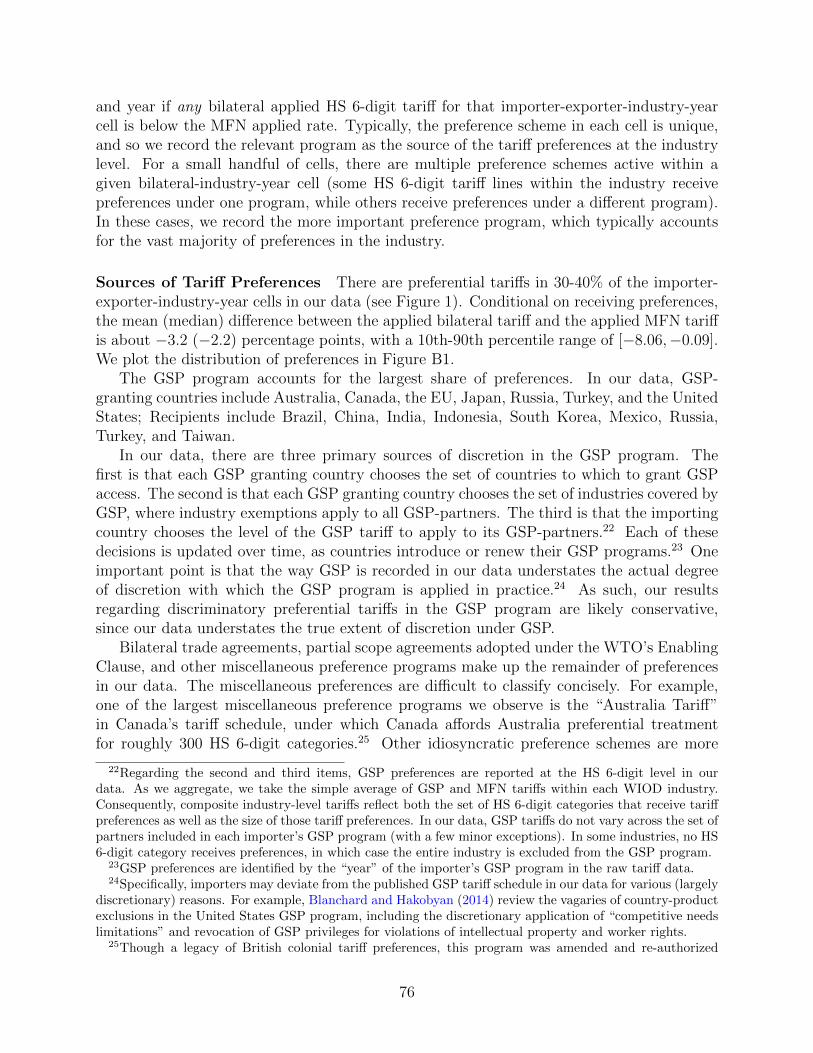
and year if any bilateral applied HS 6-digit tariff for that importer-exporter-industry-yearcell is below the MFN applied rate. Typically, the preference scheme in each cell is unique,and so we record the relevant program as the source of the tariff preferences at the industrylevel. For a small handful of cells, there are multiple preference schemes active within agiven bilateral-industry-year cell (some HS 6-digit tariff lines within the industry receivepreferences under one program, while others receive preferences under a different program).In these cases, we record the more important preference program, which typically accountsfor the vast majority of preferences in the industry.

Sources of Tariff Preferences There are preferential tariffs in 30-40% of the importer-exporter-industry-year cells in our data (see Figure 1). Conditional on receiving preferences,the mean (median) difference between the applied bilateral tariff and the applied MFN tariffis about −3.2 (−2.2) percentage points, with a 10th-90th percentile range of [−8.06,−0.09].We plot the distribution of preferences in Figure B1.

The GSP program accounts for the largest share of preferences. In our data, GSP-granting countries include Australia, Canada, the EU, Japan, Russia, Turkey, and the UnitedStates; Recipients include Brazil, China, India, Indonesia, South Korea, Mexico, Russia,Turkey, and Taiwan.

In our data, there are three primary sources of discretion in the GSP program. Thefirst is that each GSP granting country chooses the set of countries to which to grant GSPaccess. The second is that each GSP granting country chooses the set of industries covered byGSP, where industry exemptions apply to all GSP-partners. The third is that the importingcountry chooses the level of the GSP tariff to apply to its GSP-partners.22 Each of thesedecisions is updated over time, as countries introduce or renew their GSP programs.23 Oneimportant point is that the way GSP is recorded in our data understates the actual degreeof discretion with which the GSP program is applied in practice.24 As such, our resultsregarding discriminatory preferential tariffs in the GSP program are likely conservative,since our data understates the true extent of discretion under GSP.

Bilateral trade agreements, partial scope agreements adopted under the WTO’s EnablingClause, and other miscellaneous preference programs make up the remainder of preferencesin our data. The miscellaneous preferences are difficult to classify concisely. For example,one of the largest miscellaneous preference programs we observe is the “Australia Tariff”in Canada’s tariff schedule, under which Canada affords Australia preferential treatmentfor roughly 300 HS 6-digit categories.25 Other idiosyncratic preference schemes are more

22Regarding the second and third items, GSP preferences are reported at the HS 6-digit level in ourdata. As we aggregate, we take the simple average of GSP and MFN tariffs within each WIOD industry.Consequently, composite industry-level tariffs reflect both the set of HS 6-digit categories that receive tariffpreferences as well as the size of those tariff preferences. In our data, GSP tariffs do not vary across the set ofpartners included in each importer’s GSP program (with a few minor exceptions). In some industries, no HS6-digit category receives preferences, in which case the entire industry is excluded from the GSP program.

23GSP preferences are identified by the “year” of the importer’s GSP program in the raw tariff data.24Specifically, importers may deviate from the published GSP tariff schedule in our data for various (largely

discretionary) reasons. For example, Blanchard and Hakobyan (2014) review the vagaries of country-productexclusions in the United States GSP program, including the discretionary application of “competitive needslimitations” and revocation of GSP privileges for violations of intellectual property and worker rights.

25Though a legacy of British colonial tariff preferences, this program was amended and re-authorized

76

limited, sometimes covering only a few miscellaneous HS 6-digit tariff lines.Turning to bilateral trade agreements, we classify these preferences programs into two

groups, consistent with our theoretical discussion in Section 3.2.2: potentially reciprocaltrade agreements (RTAs) and non-reciprocal trade agreements.26 Our baseline approach toclassifying these agreements is as follows.

We define country i to have a potentially reciprocal trade agreement (RTA) with countryj in year t if those countries have a trade agreement in force that was notified to the WTOunder Article XXIV and is symmetrically phased in.27 In the language of Article XXIV,these are commonly referred to as Customs Unions and Free Trade Areas. Article XXIV is auseful device to classify agreements because it requires countries to eliminate tariffs/dutieson ‘substantially all trade’. This requirement is evident in practice, as these agreements havemuch broader coverage on average than other trade agreements.

We classify remaining trade agreements as non-reciprocal. These agreements are exclu-sively struck between developing countries, and most are notified to the WTO under theEnabling Clause. Because they are notified under the Enabling Clause, these agreements arenot bound by the ‘substantially all trade’ requirement of Article XXIV agreement. The dataconfirm that these agreements are much narrower in scope, often having HS 6-digit coveragerates of less than 20 percent, compared to over 90 percent for RTAs. Reflecting this differentstandard, two of these agreements (the Asia-Pacific Trade Agreement and the Global Systemof Trade Preferences) are commonly referred to as “partial scope” agreements.

Table B1 lists the trade agreements in our data, years they are in force, years they areasymmetrically phased in, and the way in which they are notified to the WTO. Again, wecode RTAijt = 1 if country i has an Article XXIV trade agreement with country j that issymmetrically phased in at date t, and zero otherwise.28

B.1.3 Temporary Trade Barriers

We draw our data from the World Bank’s Temporary Trade Barriers Database [Bown (2016)],which is available at https://www.chadpbown.com/temporary-trade-barriers-database/.In the raw data, antidumping and countervailing duties (CVDs) are explicitly partner- andproduct-specific. While safeguards are applied at the product level, they take on an exporter-

during our sample period, in 1998.26A subtle note is that our language here differs a bit from the way the WTO describes these agreements.

The WTO refers to all WTO-notified agreements as ‘reciprocal’ in that they involve the exchange of tariffpreferences. We take ‘reciprocal’ to mean a sufficiently comprehensive and symmetric exchange of tariffpreferences that nullifies bilateral terms-of-trade externalities within the agreement. There is not a strongpresumption that terms-of-trade externalities are neutralized by partial agreements, covering a minority oftrade. Whether agreements do achieve terms-of-trade neutralization is fundamentally an empirical question,which we address via our testing procedure.

27Some agreements that enter into force appear as unilateral preferences in the data, where country i grantspreferences to country j under the agreement but not vice versa. Typically j then grants preferences to iin a later year, making the agreement reciprocal. For example, for the US-Australia free trade agreement,the United States implemented preferences immediately when the agreement entered into force, whereasAustralia’s implementation of preferences was more gradual. We consider the asymmetric phase-in as adiscretionary decision, so treat it as unilateral conferral of preferences. Results are robust to re-coding theagreements as full RTAs for years in which they are asymmetrically phased in.

28For example, RTAEUN,MEX,2000 = 0 and RTAEUN,MEX,2005 = 1.

77

specific dimension via country-level exclusions. As described in Bown (2011), antidumpingand safeguards were the most heavily used of the policies for our countries during this sampleperiod. Furthermore, in the handful of cases in which CVDs were utilized, they were typ-ically applied concurrently (for the same products and exporters) with antidumping duties[Bown (2011, pp. 1989-1990)], so that our measures of TTBs would not be substantiallyaffected by dropping CVDs.

As in the tariff data, we begin with TTB data at the product-level, aggregate to theHS 6-digit level, extract HS categories that correspond to final goods, and then aggregateto WIOD industries. The TTB coverage ratio is the (unweighted) share of HS 6-digit finalgoods products within a WIOD sector for which a given importing country has a TTB ineffect against a particular trading partner in a given year.

Coverage ratios are a convenient tool for aggregating TTBs across products and mea-suring their overall intensity, which avoids needing to convert heterogeneous TTB measures(e.g., ad valorem duties, specific duties, price undertakings, or quantitative restrictions) intoad valorem equivalents. For emphasis, the coverage ratio measures the stock of TTBs inforce, not the flow of newly imposed TTBs. Further, the stock measure accounts for removalof TTBs as they expire.

78

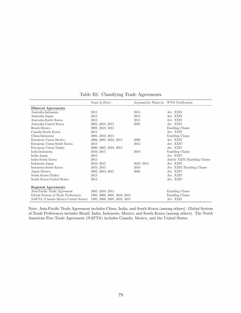
Table B1: Classifying Trade Agreements

Years in Force Asymmetric Phase-in WTO Notification

Bilateral AgreementsAustralia-Indonesia 2015 2015 Art. XXIVAustralia-Japan 2015 2015 Art. XXIVAustralia-South Korea 2015 2015 Art. XXIVAustralia-United States 2005, 2010, 2015 2005 Art. XXIVBrazil-Mexico 2005, 2010, 2015 Enabling ClauseCanada-South Korea 2015 Art. XXIVChina-Indonesia 2005, 2010, 2015 Enabling ClauseEuropean Union-Mexico 2000, 2005, 2010, 2015 2000 Art. XXIVEuropean Union-South Korea 2015 2015 Art. XXIVEuropean Union-Turkey 2000, 2005, 2010, 2015 Art. XXIVIndia-Indonesia 2010, 2015 2010 Enabling ClauseIndia-Japan 2015 Art. XXIVIndia-South Korea 2015 Article XXIV/Enabling ClauseIndonesia-Japan 2010, 2015 2010, 2015 Art. XXIVIndonesia-South Korea 2010, 2015 2010 Art. XXIV/Enabling ClauseJapan-Mexico 2005, 2010, 2015 2005 Art. XXIVSouth Korea-Turkey 2015 Art. XXIVSouth Korea-United States 2015 Art. XXIV

Regional AgreementsAsia-Pacific Trade Agreement 2005, 2010, 2015 Enabling ClauseGlobal System of Trade Preferences 1995, 2000, 2005, 2010, 2015 Enabling ClauseNAFTA (Canada-Mexico-United States) 1995, 2000, 2005, 2010, 2015 Art. XXIV

Note: Asia-Pacific Trade Agreement includes China, India, and South Korea (among others). Global Systemof Trade Preferences includes Brazil, India, Indonesia, Mexico, and South Korea (among others). The NorthAmerican Free Trade Agreement (NAFTA) includes Canada, Mexico, and the United States.

79

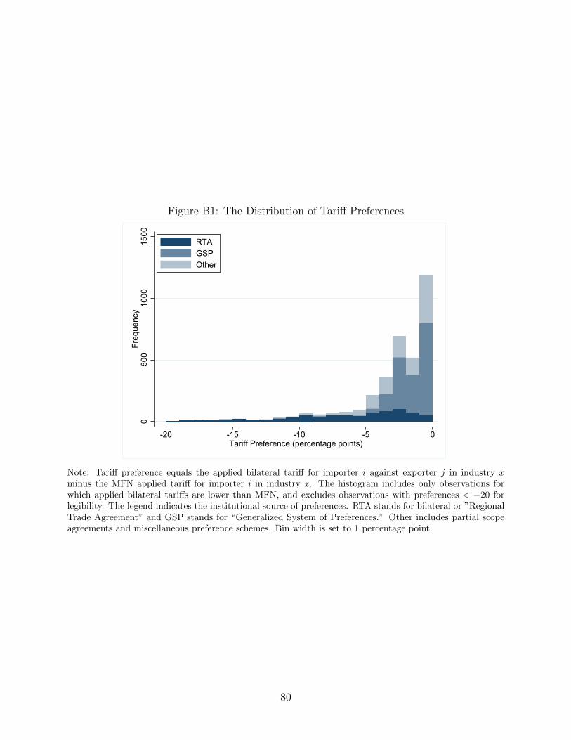
Figure B1: The Distribution of Tariff Preferences

050

010

0015

00Fr

eque

ncy

-20 -15 -10 -5 0Tariff Preference (percentage points)

RTAGSPOther

Note: Tariff preference equals the applied bilateral tariff for importer i against exporter j in industry xminus the MFN applied tariff for importer i in industry x. The histogram includes only observations forwhich applied bilateral tariffs are lower than MFN, and excludes observations with preferences < −20 forlegibility. The legend indicates the institutional source of preferences. RTA stands for bilateral or ”RegionalTrade Agreement” and GSP stands for “Generalized System of Preferences.” Other includes partial scopeagreements and miscellaneous preference schemes. Bin width is set to 1 percentage point.

80

B.2 Supplemental Appendix: Empirical Strategy and Results

In this appendix, we provide supplemental discussion of the empirical results. First, wediscuss details about how we measure upstream production differentiation for use in Section4.2.2. Second, we explore several variations on the instrumental variables results presentedin the main text, which make use of different instruments and empirical specifications.

B.2.1 Measuring Upstream Differentiation

In Section 4.2.2, we discuss heterogeneity in coefficient estimates, depending on the degreeof upstream differentiation. We include details related to these exercises here.

To formalize the argument for measuring upstream differentiation, we defined the pass-

through elasticity as εjxh ≡drjxhdpjx

dpjxrjxh

. This is the elasticity of the price of value added from

country h used by sector x in country j. Extending the theory to distinguish upstream inputsupply sectors, suppose that vjxh is a bundle of factors vzjxh, where z distinguishes underlying

factor types, with associated prices rzjxh and pass-through elasticities εzjxh ≡drzjxhdpjx

dpzjxrzjxh

. Then

the aggregate, bilateral pass-through elasticity is: εjxh =∑

z

(DV AzjxhDV Ajxh

)εzjxh, where DV Azjxh ≡

rzjxhvzjxh.

Then, suppose there are two types of factors, those with high (H) pass-through elastic-ities and others with low (L) pass-through elasticities: εHjsh , ε

Ljsh. Then we decompose the

aggregate elasticity as follows:

εjxh = εHjxh

(DV AHjxhDV Ajxh

)+ εLjxh

(DV ALjxhDV Ajxh

), (B1)

where DV AHjxh ≡∑

z∈H DV Azjxh and DV ALjxh =

∑z∈LDV A

zjxh. With this decomposition, the

DVA-specific term in the optimal bilateral tariff becomes:

(1 + δ∗xh)εjxh

DV AjxhpjxMh

xj

= (1 + δ∗xh)

[εHjxh

(DV AHjxhDV Ajxh

)+ εLjxh

(DV ALjxhDV Ajxh

)]DV AjxhpjxMh

xj

= (1 + δ∗xh)εHjxh

DV AHjxhpjxMh

xj

+ (1 + δ∗xh)εLjxi

DV ALjxhpjxMh

xj

.

(B2)

This decomposition motivates our effort to measure DV AHjxh and DV ALjxh separately, and

then construct ln

(DV AHjxhpjxM

hxj

)and ln

(DV ALjxhpjxM

hxj

). Coefficients attached to these separate DVA

ratios then shed light on underlying pass-through elasticities εHjxh versus εLjxh.As discussed in the text, we take two different approaches. The first approach is is to

classify manufacturing sectors as differentiated, high pass-through sectors (H) and all othersectors as low pass-through sectors L. Then DV AHjxh is value added that originates in themanufacturing sector of country h that is used by industry x in country j, and DV ALjxh isvalue added from non-manufacturing sectors.

81

The second approach uses the Rauch classification [Rauch (1999)]. Rauch classifiescommodities as differentiated or non-differentiated at the SITC 4-digit level. We concordthese to WIOD industries, where there are many SITC industries (k) in each WIOD in-dustry. Letting diffk = 1 if SITC category k is differentiated, and 0 otherwise, we theconstruct the share of underlying SITC categories that are differentiated within each WIODindustry, denoted by z: diffz ≡ 1

Kz

∑k∈z diffk. Then we decompose DVA as follows:

DV Ajxh = DV ARjxh +DV A(−R)jxh , where DV ARjxh =

∑z diffzDV A

zjxh is value added that orig-

inates in Rauch differentiated sectors, and DV A−Rjxh = DV Ajxh−DV ARjxh is value added that

originates in non-differentiated sectors.

B.2.2 Supplemental IV Results

As noted at the end of Section 4.3, we examine several alternative approaches to instrumentalvariables estimation, which supplement the analysis in the text. First, we swap out theinstrument for imports, replacing the instrument based on heterogeneous distance effects withan alternative instrument based on predetermined values of imports. Second, we consider analternative instrument for domestic GVC income in foreign production (DV Ahxjt), similarlybased on predetermined values. Third, we examine an alternative regression specificationin which imports are treated as a nuisance control, absorbed by decile fixed effects thatnon-parametrically control for the volume of imports. This final exercise is closely relatedto a specification we used in Blanchard, Bown and Johnson (2016) to estimate the influenceof domestic GVC income on tariffs. We describe these approaches in greater detail below.The takeaway is that these alternative IV strategies all yield results consistent with theIV estimation presented in the main text, which supports the causal interpretation of ourresults.

Alternative Instrument for Imports Recall that the endogeneity concern for imports isthat they are simultaneously determined by tariffs, so that residual variation in tariff prefer-ences that is not accounted for by the model may be correlated with imports. One approachto resolving this concern would be to use imports from periods prior to the introduction ofthe tariff preferences in our data as an instrument for current imports. Since these prede-termined import values cannot mechanically be a function of residual tariff preferences, thisresolves the simultaneity problem.

Since no preference programs in our data were in force in 1970, then imports from 1970would satisfy the necessary exclusion restriction. To construct the instrument, we obtainbilateral trade data for 1970 at the SITC 4-digit (Rev. 2) level from the NBER-UnitedNations Trade Data [Feenstra et al. (2005)]. We extract SITC categories corresponding tofinal goods using the BEC classification, and then concord SITC categories to our WIODindustries via ISIC industries.29 This process gives us imports of final goods by importer,

29Because country definitions have changed over time, we concord historical countries to modern entitiesas best we can. For example, Germany today corresponds most closely to the former Federal Republic ofGermany. Russia today corresponds to the former USSR. And so on. Further, more trade flows in theNBER-UN data are zero in 1970 than are zero today, likely due both to true changes from zeros to positivevalues over time and differences in reporting thresholds and/or missing data in the two data sources. Inorder to use the whole sample, we replace zeros in 1970 with the smallest values observed in the data.

82

exporter, and industry in 1970.With this data in hand, we construct three instruments, one for each of the ratios in

Equation (3.7). The first is the log difference between DVA-in-Services and the value ofimports in 1970 by country pair and industry. The second and third are the log differencesbetween the shift-share instruments (described in Section 4.3) for final goods production andFVA and the value of imports in 1970 by country pair and industry.30

The benchmark IV results are replicated with this instrument set in Table B2.31 Wefind the same signs for the main coefficients as in OLS and Table 6. The coefficient for theDVA ratio is similar in magnitude to that in Table 6. The coefficients on the FVA and IPRatios are pushed away from zero, though they are imprecisely estimated, so we hesitate toover-interpret the magnitude of the point estimates.

Alternative Instrument for DVA In Table 6, we used DVA in an outside sector (theservices sector) as the instrument. Now we consider a different instrument, based on a distinctidentification argument. Specifically, we again note that the identification concern in themodel centers on the simultaneity problem, in which DV Ahxjt may be endogeneously relatedto residual variation in tariff preferences (exhjt). As in the discussion above, predeterminedvalues ofDV Ahxjt would serve as a valid instrument; since they are determined to introductionof the preferences in our data, they cannot mechanically be a function of them, and thuswould satisfy the exclusion restriction.

To construct this instrument, we use data on the level of domestic value-added contentin foreign production in 1970, which we denote DV Ahsj,1970 and verbally refer to as DVA-in-1970. Drawing on the data set developed in Johnson and Noguera (2017), we measureDVA-in-1970 for two composite sectors: agriculture and manufacturing. Due to missing datafor Russia and Taiwan, the sample for which we can construct this instrument is roughly30 percent smaller than our baseline sample. This is one cost of using this instrument.A second cost is that there is no time-variation in the instrument, in contrast to DVA-in-Services. On the other hand, this cost is counterbalanced by additional cross-industryvariation in this instrument; this instrument isolates different exogenous variation than doesthe DVA-in-Services instrument. The final cost of this instrument is that is generally weak inthe specifications we used in Table 6. However, it does potentially contain useful informationto corroborate the main analysis.

In Table B3, we replicate results from Panel A of Table 6 using DVA-in-1970 as theinstrument, where we use the same instrument for imports as in the main text. Lookingat the Weak-Identification Test statistic, it is evident that the instruments are sufficientlyweak to be concerned about using conventional standard errors for inference. Thus, while wereport conventional standard errors in parentheses, we omit stars associated with significancetests. We also caution against parsing the point estimates.

More reassuringly, the DVA-in-1970 instrument is powerful enough in this specification to

30Note here that we avail ourselves of the ability to use the log ratios as instruments, which was notpossible with the heterogeneous distance instrument used in the main text. In practice, this improves thepower of the instrument set, relative to including log levels of these variables separately as instruments.

31We focus on the main IV results, omitting auxiliary controls. The reason is that this instrument set isagain weak when controls are added, likely because the controls absorb variation in imports in 1970. Further,as in the main text, adding controls does not qualitatively change the results.

83

make statistical inferences. Specifically, we construct and report weak-IV robust confidenceintervals for the key coefficient attached to the log DVA ratio in brackets in the table. Theseare based on inversion of the Anderson-Rubin test static with 10% nominal size, under theassumption that γIP + γFV A is strongly identified.32 The key point is that these confidenceintervals contain only negative values, so we can again conclude that higher DVA is associatedwith lower tariffs. Though the estimates are imprecise, this instrument corroborates thecausal interpretation of the main results.

Alternative IV Specification to Estimate DVA Effects The final exercise we conductchanges the way in which we control for bilateral imports. Referring back to Equation (3.5),we note that the imports enter the expression evaluated at the baseline no-GVC equilibrium.We introduce observed imports into the estimation framework [Equations (3.6)-(3.7)] as aproxy for these unobserved values. However, we could alternatively attempt to simply controlfor unobserved imports in a nonparameteric way.

To implement this idea, we divide the observed empirical distribution of imports intoten decile bins and form indicators Dxijt ≡ 1(pixtM

ixjt ∈ D), where D indexes the set of

import decile bins. We can then include these indicators as control variables to proxy forunobserved variation in imports in the no-GVC equilibrium, along with the log levels ofthe other independent variables. As in Blanchard, Bown and Johnson (2016), we focus onestimating DVA effects in this specification, so the empirical estimation includes importer-industry-year fixed effects. This yields the following empirical specification:

thxjt − th,MFNxt = φxht + φxjt +Dxijt + γDV A ln

(DV Ajxht

)+ exhjt, (B3)

We then instrument ln(DV Ajxht

)using either the DVA-in-Services instrument from the main

text, or the DVA-in-1970 instrument discussed above.In Panel A of Table B4, we report results that use DVA-in-Services as the instrument.

In Panel B of Table B4, we then repeat the estimation with DVA-in-1970 as the instrument.For both instruments, estimates for the coefficient on the log DVA ratio are negative, theyare robust across specifications with varying control variables, and they generally consistentin magnitude with those reported elsewhere. We conclude that this evidence again supportsthe causal interpretation of the estimates in the main body of the paper.

32This assumption seems reasonable, based on the fact that the heterogeneous distance elasticity instru-ment for imports does not appear weak in specifications reported in the main text, when combined with theDVA-in-Services instrument. If we drop this assumption and assume both are weak, then the confidenceintervals for the log DVA ratio are unbounded on the left (for reasonable minimum grid search values),though they are still bounded on the right by negative values – i.e., we can reject that the coefficient iszero or positive. The unboundedness of the confidence set is a common issue in construction of weak-IVconfidence intervals based on the AR statistic, which suffers from poor power. Conditioning on the strongidentification of γIP + γFV A serves to enhance the power of the test. See Section 5.3 of Andrews, Stock andSun (2019) for a concise discussion of these issues.

84

Table B2: IV Estimates using Alternative Instruments for Imports

OLS Instrumental Variables

(1) (2) (3) (4)

DVA ratio: ln(DV Ajxht/IMhxjt) -0.98*** -1.09*** -1.49** -1.47**

(0.27) (0.30) (0.66) (0.68)FVA ratio: ln(FV Ahxt/IM

hxjt) -0.97*** -14.41**

(0.23) (5.76)IP ratio: ln(FGh

xt/IMhxjt) 2.13*** 15.85**

(0.48) (6.09)IP ratio + FVA ratio (γIP + γFV A) 1.29*** 1.43***

(0.33) (0.38)

Observations 11,281 11,281 11,281 11,281Under-Identfication Test (rk LM statistic) 29.12 20.22Weak-Identfication Test (Wald rk F statistic) 11.92 11.77Conditional F-Stat (DVA ratio) 25.18 23.78Conditional F-Stat (FVA ratio) 48.78Conditional F-Stat (FG ratio) 48.49Conditional F-Stat (IP ratio + FVA Ratio) 51.27

Column Fixed Effects

Importer-Year Y N Y NImporter-Industry Y N Y NImporter-Industry-Year N Y N YExporter-Industry-Year Y Y Y Y

Note: Columns (1)-(2) repeat OLS results from Table 2 for reference. Instrumental variables results areobtained via two-stage least squares, where instruments are constructed using imports in 1970 to constructthe ratios; see section titled “Alternative Instrument for Imports.” Standard errors (in parentheses) areclustered by importer-exporter pair. Significance levels: * p < .1, ** p < .05, *** p < .01. Under/Weak-Identification Tests are based on Kleinbergen and Paap (2006) and conditional F-statistics are based onSanderson and Windmeijer (2016).

85

Table B3: IV Estimates with Alternative Instrument for DVA

OLS Instrumental Variables

(1) (2) (3) (4)

DVA ratio: ln(DV Ajxht/IMhxjt) -0.95*** -8.85 -8.57 -7.85

(0.32) (4.63) (4.46) (4.15)[-27.58,-5.38] [-26.61,-5.23] [ -25.88,-4.74]

IP ratio + FVA ratio (γIP + γFV A) 1.13*** 5.02 4.78 4.18(0.35) (2.96) (2.87) (2.66)

Log Bilateral Distance 0.81** -0.66 -0.33 -0.89(0.37) (1.91) (2.03) (1.72)

Colony 2.17 -0.12(2.96) (2.53)

Common Language -0.31 0.14(1.38) (1.22)

Contiguity -0.01 1.13(2.31) (2.34)

Reciprocal Trade Agreement: RTAhjt -4.58(1.37)

Observations 8,520 8,520 8,520 8,520Under-Identfication Test (rk LM statistic) 5.662 5.896 5.726Weak-Identfication Test (Wald rk F statistic) 2.793 2.947 2.845Conditional F-Stat (DVA ratio) 6.951 7.291 7.181Conditional F-Stat (IP ratio + FVA ratio) 6.661 6.944 6.821

Note: Columns (1) includes OLS result for the sub-sample for which the DVA-in-1970 instrument is available.Instrumental variables results are obtained via two-stage least squares. Under/Weak-Identification Tests arebased on Kleinbergen and Paap (2006) and conditional F-statistics are based on Sanderson and Windmeijer(2016). For all columns, conventional standard errors (in parentheses) are clustered by importer-exporterpair. For columns (1), significance levels: * p < .1, ** p < .05, *** p < .01. For columns (2)-(4) starsto indicate significance levels are omitted, due to concerns about weak instruments. For the DVA ratio,weak-IV robust confidence intervals are reported in brackets, based on inversion of the Anderson-Rubin teststatic with 10% nominal size under the assumption that γIP + γFV A is strongly identified.

86

Table B4: Alternative IV Specification: Decile Indicator Controls for Imports

Panel A: DVA-in-Services

(1) (2) (3) (4)

DVA: ln(DV Ajxht) -1.26*** -0.81** -0.63** -0.43**(0.35) (0.33) (0.27) (0.20)

Log Bilateral Distance 0.77** 0.95*** 0.25(0.30) (0.33) (0.22)

Colony 2.28*** 0.37(0.72) (0.38)

Common Language 0.21 0.54(0.53) (0.47)

Contiguity -1.30 0.34(1.12) (1.06)

Reciprocal Trade Agreement: RTAhjt -5.57***(0.89)

Observations 11,281 11,281 11,281 11,281Under-Identfication Test (rk LM statistic) 61.46 62.14 58.31 56.39Weak-Identfication Test (Wald rk F statistic) 2497 1213 1076 1048

Panel B: DVA-in-1970

(5) (6) (7) (8)

DVA: ln(DV Ajxht) -2.14*** -2.16** -2.16** -1.65*(0.48) (0.90) (1.02) (0.85)

Log Bilateral Distance -0.03 0.12 -0.49(0.75) (0.98) (0.72)

Colony 2.84** 0.28(1.23) (0.79)

Common Language 0.03 0.49(0.71) (0.61)

Contiguity -0.69 0.58(1.33) (1.33)

Reciprocal Trade Agreement: RTAhjt -5.07***(0.96)

Observations 8,520 8,520 8,520 8,520Under-Identfication Test (rk LM statistic) 34.28 15.61 13.61 13.54Weak-Identfication Test (Wald rk F statistic) 62.98 22.37 20.61 20.03

Note: Instrumental variables results are obtained via two-stage least squares. Under/Weak-IdentificationTests are based on Kleinbergen and Paap (2006) and conditional F-statistics are based on Sanderson andWindmeijer (2016). Standard errors (in parentheses) are clustered by importer-exporter pair. Significancelevels: * p < .1, ** p < .05, *** p < .01.

87