Global priorities for conserving the evolutionary history ... · In tmrrmstriil Xmrtmjritms,...

Articleshttps://doi.org/10.1038/s41559-017-0448-4

© 2018 Macmillan Publishers Limited, part of Springer Nature. All rights reserved.

1Department of Biological Sciences, Simon Fraser University, Burnaby, British Columbia, Canada. 2Scimitar Scientific, Whitehorse, Yukon, Canada. 3Biology Department, St Ambrose University, Davenport, IA, USA. 4BC Centre for Excellence in HIV/AIDS, University of British Columbia, Vancouver, British Columbia, Canada. 5Department of Medicine, University of British Columbia, Vancouver, British Columbia, Canada. R. William Stein and Christopher G. Mull contributed equally to this work. *e-mail: [email protected]; [email protected]; [email protected]

The global extinction crisis is a wicked problem—it is gener-ally accepted that prioritization is necessary due to limited resources and an expanding list of threatened species to save1–4.

Various prioritization goals and frameworks exist, but one clear goal of biological conservation is to maximally preserve the tree of life5,6. A key priority is identifying evolutionarily isolated species with few close relatives that consequently embody a greater share of unique evolutionary history7. With rapid developments in phylogenetic inference for major taxonomic groups, we now have the tools for ranking species based on evolutionary isolation.

Evolutionary isolation is a useful metric for placing the current biodiversity crisis in a historical context and for identifying pri-ority species and places in combination with other prioritization criteria. Every year, the chondrichthyan tree accumulates ~1,200 years of unique evolutionary history, yet the modern extinction of a single species would prune tens to hundreds of millions of years of evolutionary history. Furthermore, identifying locations of high evolutionary isolation can potentially capture areas of unique forms, functions and genomes8. The International Union for the Conservation of Nature (IUCN) Red List assessments9 provide spe-cies-specific threat statuses and geographic distribution maps that can be combined with taxon-complete phylogenies to identify the most imperiled species and places that embody significant amounts of unique evolutionary history. This combined prioritization frame-work is the focus of one international conservation endeavour (Evolutionarily Distinct and Globally Endangered (EDGE): http://www.edgeofexistence.org) and has been applied, almost exclusively, to terrestrial vertebrate lineages including mammals10, amphib-ians11, birds8 and, most recently, squamates12. Applying this EDGE approach to a marine vertebrate lineage will address a key ques-tion—what is the taxonomic and geographic distribution of evolu-tionary distinctness (ED) in the oceans?

Here, we apply the EDGE approach to the sharks, rays and chi-maeras (class Chondrichthyes), one of only two extant divisions

of jawed vertebrates and one of the three classes of fishes. Chondrichthyans fill a range of ecological roles, most notably func-tioning as apex and mesopredators in the upper trophic levels of oceanic, nearshore and freshwater food webs13,14, helping to shape and control food web structure15,16. Chondrichthyans also provide an important perspective to interpreting functional and life history evolution as the sister group to all other extant jawed vertebrates (Gnathostomes). For example, they mark the appearance of the ver-tebrate brain archetype17 and many species give birth to live young nourished through a placenta or other forms of maternal invest-ment18. Importantly, chondrichthyans are among the most-imper-iled marine organisms19, with up to a quarter facing an increased risk of extinction20.

First, we ranked all 1,192 shark, ray and chimaera species by their evolutionary isolation, measured as ED10,21 using recently developed methods for combining time-calibrated molecular phylogenies with taxonomic information to produce distributions of robust taxon-complete trees22,23 (Fig. 1). Second, we combined ED with imperiled status (species threatened or predicted to be threatened)20, life his-tory and ecological traits, and geographic distributions. We asked five questions: (1) Which are the most evolutionary distinct lin-eages of all the major vertebrate radiations? (2) Which are the most imperiled evolutionary distinct species, the extinction of which would lead to disproportionate losses of chondrichthyan evolution-ary history? (3) Is ED and extinction risk driven more by species’ life history and ecological traits or their underlying evolutionary phylogenetic relationships? (4) Where are the global locations that harbour the greatest ED? Finally, (5) where are the places that har-bour the trifecta of greatest species richness, greatest endemism and greatest richness of the most evolutionarily distinct species?

ResultsED across major vertebrate radiations. The total evolutionary his-tory (the sum of all branch lengths and also sum of all ED scores)

Global priorities for conserving the evolutionary history of sharks, rays and chimaerasR. William Stein1, Christopher G. Mull 1*, Tyler S. Kuhn2, Neil C. Aschliman3, Lindsay N. K. Davidson1, Jeffrey B. Joy4,5, Gordon J. Smith1, Nicholas K. Dulvy 1* and Arne O. Mooers 1*

In an era of accelerated biodiversity loss and limited conservation resources, systematic prioritization of species and places is essential. In terrestrial vertebrates, evolutionary distinctness has been used to identify species and locations that embody the greatest share of evolutionary history. We estimate evolutionary distinctness for a large marine vertebrate radiation on a dated taxon-complete tree for all 1,192 chondrichthyan fishes (sharks, rays and chimaeras) by augmenting a new 610-species molecu-lar phylogeny using taxonomic constraints. Chondrichthyans are by far the most evolutionarily distinct of all major radiations of jawed vertebrates—the average species embodies 26 million years of unique evolutionary history. With this metric, we identify 21 countries with the highest richness, endemism and evolutionary distinctness of threatened species as targets for conser-vation prioritization. On average, threatened chondrichthyans are more evolutionarily distinct—further motivating improved conservation, fisheries management and trade regulation to avoid significant pruning of the chondrichthyan tree of life.

NATuRe eCOLOGy & evOLuTiON | www.nature.com/natecolevol

https://doi.org/10.1038/s41559-017-0448-4

mailto:[email protected]



http://www.edgeofexistence.org

http://www.edgeofexistence.org

http://orcid.org/0000-0003-1710-8256

http://orcid.org/0000-0002-4295-9725

http://orcid.org/0000-0003-0383-8856

http://www.nature.com/natecolevol

© 2018 Macmillan Publishers Limited, part of Springer Nature. All rights reserved. © 2018 Macmillan Publishers Limited, part of Springer Nature. All rights reserved.

Articles Nature eCOlOgy & evOlutION

encompassed in the chondrichthyan tree is 36,840 Myr (5th and 95th centiles: 21,812–60,108; Fig. 1). Evolutionary isolation, as measured by ED, is log-normally distributed with the median chondrichthyan embodying 26 Myr of ED (5th and 95th centiles: 13–64 Myr; Fig. 2a). Indeed, among the major radiations of liv-ing vertebrates, and with the exception of two living fossil lineages (the coelacanths and the lungfishes), only the jawless hagfishes and lampreys (Agnatha) embody more evolutionary history per species than the average chondrichthyan. An average shark, ray or chimaera is likely to represent more than twice the evolutionary history of an average amphibian (10.1 Myr) or squamate reptile (11.1 Myr), three times the history of an average mammal (8 Myr) and four times the history of the average bird species (6.2 Myr; Fig. 2a).

Taxonomic distribution of ED across chondrichthyans. There is surprisingly consistent average ED among the four main super-ordinal lineages within Chondrichthyes, despite their widely differ-ing species richness (chimaeras, Holocephali median ED = 40 Myr; sharks, Squalomorphii 36 Myr, Galeomorphii 33 Myr; rays, Batoidea 28 Myr; Fig. 2b), while averages across orders vary consid-erably (Fig. 2b). In particular, two radiations comprise numerous, relatively low-ED species: skates (Rajiformes, 293 species, median ED = 17 Myr) and ground sharks (Carcharhiniformes, 281 species, median ED = 24 Myr). Conversely, two depauperate lineages con-tain high-ED species: mackerel sharks (Lamniformes, 15 species, median ED = 64 Myr) and cow sharks (Hexanchiformes, 7 species, median ED = 79 Myr; Fig. 2b).

Two orders are characterized by both a high median ED and a high percentage of threatened species, making them of poten-tially high conservation concern: mackerel sharks (Lamniformes) and guitarfishes, wedgefishes and sawfishes (Rhinopristiformes).

Mackerel sharks comprise 15 species of mainly large pelagic sharks, 10 of which are threatened due to longline fisheries targeting tuna and billfishes. The extinction of a single species within this group could result in a median loss of 64 Myr of evolutionary history (as measured by ED). Guitarfishes, wedgefishes and sawfishes comprise 59 species of moderate-to-large coastal benthopelagic species, 29 of which are threatened due to their retention in nearshore trawl and gillnet fisheries. An extinction within this group could result in a median loss of 37 Myr of evolutionary history.

High- and low-ED lineages are distributed throughout the 14 chondrichthyan orders (Fig. 3a). The lowest-ED species are found within the skate genus Bathyraja (three species with median ED = 7.4 Myr) while the single most evolutionarily distinct species is the striped panray (Zanobatus schoenleinii; median ED = 188 Myr; Fig. 3b). The 120 species in the top 10% ED are drawn from 13 out of 14 orders—only the angel sharks (Squatiniformes) are not repre-sented—and 45 of 60 families. Together, these top 10% ED species embody 8,581 Myr, or 23%, of total ED.

The 20 most evolutionarily distinct species include some unique ecomorphological specializations that would be lost with their extinction. The top three ED species are rays: striped panray, cof-fin ray (Hypnos monopterygius) and sixgill stingray (Hexatrygon bickelli; Fig. 3b). The top three sharks are all members of the spe-cies-poor and high-ED order of mackerel sharks (Lamniformes): goblin shark (Mitsukurina owstoni; ranked 4th overall), sandtiger shark (Carcharias taurus; 8th) and bigeye thresher (Alopias super-ciliosus; 9th; Fig. 3b). It is important to highlight that 3 of the top 20 ED are Data Deficient: the striped panray, broadnose sevengill shark (Notorynchus cepedianus) and viper dogfish (Trigonognathus kabeyi; Fig. 3b). The top 20 most evolutionarily distinct and threat-ened species includes all five sawfishes in the family Pristidae—three

Molecular data coverage (%)within order

Rajiformes

Molecular data

Pristiophoriformes

Echinorhiniformes

SqualiformesSquatiniformes

Heterodontiformes

Orectolobiformes

Lamniformes

Carcharhiniformes

20 40 60 80 100

Myliobatiformes

Hexanchiformes

Chimaeriformes

RhinopristiformesTorpediniformes

Fig. 1 | A representative taxon-complete tree with phylogenetic distribution of molecular data coverage. Clades are shaded according to molecular data coverage within each order, and those species with molecular data are indicated by outer ticks. Red dots highlight nodes defining orders, with the paraphyletic order Rhinopristiformes delimited by two highly supported nodes.




ArticlesNature eCOlOgy & evOlutION

species are Critically Endangered and two are Endangered mak-ing them one of the most threatened families of marine fishes20. There are eight threatened high-ED sharks, including: fos-sil shark (Hemipristis elongata; 19th), broadnose sevengill shark (Notorynchus cepedianus; 11th), Colclough’s shark (Brachaelurus colcloughi; 16th), horn shark (Heterodontus francisci; 38th) and white shark (Carcharodon carcharias; 42th). The remaining seven imperiled high-ED rays include: sharkray (Rhina ancyclostoma; 10th), two guitarfishes (Zapteryx spp.), two eagle rays (Aetobatus spp.), as well as two fanrays (Platyrhina spp.; Fig. 3c). An additional three species in the top 20 ED and threatened are Data Deficient: banded guitarfish (Zapteryx exasperata), hyuga fanray (Platyrhina hyugaensis) and horn shark (Fig. 3c). We also flag some recently radiated, low ED, endemic skates and freshwater sharks that are highly threatened (Supplementary Data).

Traits, extinction risk and the likely loss of evolutionary history. A key conservation concern is whether extinction risk covaries with ED; if so, then overfishing—the main threat to marine bio-diversity24,25—may result in a disproportionate loss of evolutionary history. The most widely accepted system for estimating extinction risk is the IUCN Red List26,27. Here, we defined imperiled species as those 179 chondrichthyans categorized by the IUCN Red List as Critically Endangered, Endangered or Vulnerable, plus the 63 Data Deficient species predicted to be threatened based on correlates of IUCN threat status20. Of the 1,192 species considered here, we rank the 242 imperiled species by median ED. The Lamniformes (mack-erel sharks) and Rhinopristiformes (guitarfishes, wedgefishes and sawfishes) dominate the top 20 imperiled species list (Fig. 3c). Taken together, these 242 imperiled species embody 8,875 Myr (24%) of

the total ED of the group. On average, imperiled chondrichthyans embody significantly more ED—7 to 8 Myr more—than non-threat-ened chondrichthyans (phylogenetic analysis of variance, all spe-cies: t = 4.73, d.f. = 359, P < 0.0001; sharks only: t = 3.22, d.f. = 136, P < 0.01; rays only: t = 6.42, d.f. = 236, P < 0.0001). This pattern con-trasts with the lack of covariation between threat status and ED in mammals28, birds8 and squamates12. This suggests that overfishing is endangering not just a disproportionate number of species in this group, but also a disproportionate fraction of evolutionary history.

We also find that life history and ecological traits associated with threat risk are correlated with ED, but these interrelation-ships vary between sharks and rays. Previous work has revealed that chondrichthyans with larger body size, shallow depth distri-butions—and hence greater exposure to fisheries—and greater extent of occurrence (EOO)20, 29,30 are more likely to be threatened. Across all chondrichthyans, greater ED was found in species with larger body size (generalized linear model, β = 0.07 ± 0.02 s.e.), shallower depth (β = − 0.09 ± 0.01) and larger geographic range size (EOO; β = 0.05 ± 0.01; Fig. 4a–c; Akaike’s information criterion (AIC) = − 265). These life history and ecological traits and ED show strong phylogenetic patterning (Supplementary Methods), such that phylogenetically corrected models have considerably lower AIC scores (phylogenetic generalized least squares average model AIC = − 1,800 for resolved 1,192 species trees; AIC = − 840 for molecular 610 spe-cies trees).

These ED–trait relationships differ between the two major lineages. Within sharks, only larger maximum body size (β = 0.13 ± 0.03) and larger EOO (β = 0.03 ± 0.01) were related to higher ED (Fig. 4d–f; AIC = − 270). These relationships are partially driven by the large-bodied, oceanic-pelagic, high-ED mackerel

a b

Expected

Observed

0–1011–2021–3031–4041–5051–6061–70

Percentthreatened

Aves

Mammalia

Squamata

Testudines

Crocodilia

Amphibia

Actinopterygii

Chondrichthyes

Agnatha

Holocephali

Chimariformes

BatoideaRajiformes

Myliobatiformes

Torpediniformes

Rhinopristiformes

SqualomorphiiSqualiformes

Squatiniformes

Pristiophoriformes

Echinorhiniformes

Hexanchiformes

GaleomorphiiCarcharhiniformes

Orectolobiformes

Heterodontiformes

Lamniformes

0 10 20 30 40 50 60 70 80 90 100 1100 10 20 30 40 50 60 70

ED (Myr)ED (Myr)

Fig. 2 | expected and observed eD. a, Across major vertebrate radiations. Large circles represent expected average ED while small circles represent the mean ED observed from taxon complete phylogenies. b, Among chondrichthyan orders. Boxplots denote median (solid line), 25th and 75th centiles (box edges), and 5th and 95th centiles (whiskers). The colour of silhouettes denotes the percentage of threatened species within each radiation or order.





Critically EndangeredEndangeredVulnerableNear ThreatenedLeast Concern

ThreatenedNot Threatened

Red List status (known)

Red List status (predicted)

ED (Myr)

20 Frill shark(Hex)

19 Fossil shark(Car)

18 Viper dogfish(Squ)

17 Blind shark(Ore)

16 Colclough’s shark(Ore)

15 Sixgill shark(Pri)

14 Basking shark(Lam)

13 Largetooth sawfish(Rhi)

12 Barbled houndshark(Car)

11 Broadnose sevengill shark(Hex)

10 Shark ray(Rhi)

9 Bigeye thresher shark(Lam)

8 Sandtiger shark(Lam)

7 Giant stingaree(Myl)

6 Narrow sawfish(Rhi)

5 Thornback ray(Tor)

4 Goblin shark(Lam)

3 Sixgill stingay(Myl)

2 Coffin ray(Tor)

1 Striped panray(Rhi)

ED (Myr)

42 White shark(Lam)

39 Ornate eagleray(Myl)

38 Hornshark(Het)

34 Fanray(Tor)

32 Hyuga fanray(Tor)

30 Green sawfish(Rhi)

29 Smalltooth sawfish(Rhi)

27 Loggerheaded eagleray(Myl)

26 Shortnose guitarfish(Rhi)

25 Banded guitarfish(Rhi)

23 Dwarf sawfish(Rhi)

19 Fossil shark(Car)

16 Colclough’s shark(Ore)

14 Basking shark(Lam)

13 Largetooth sawfish(Rhi)

11 Broadnose sevengill shark(Hex)

10 Shark ray(Rhi)

9 Bigeye thresher shark(Lam)

8 Sandtiger shark(Lam)

6 Narrow sawfish (Rhi)

cb

a 148 9

41716

38

18

151120

42

12

19

0.750.500.250.00

6 15 37 95 241Myr

7

39271 329

302313

6

102625

5 23234

50 100 150 200 250 50 100 150 200 250

Fig. 3 | Distribution of eD. a, A representative taxon-complete phylogenetic tree of all chondrichthyans. Branch colour represents the ED (in Myr) of lineages based on the colour-ramp legend, where blue is low ED and red is high ED. Numbers indicate the species highlighted, with red denoting threatened species. b, The top 20 species overall. c, The top 20 imperiled species. Boxplots denote median (solid line), 25th and 75th centiles (box edges), and 5th and 95th centiles (whiskers). Boxplot colours represent threat status, with the green to red colours depicting assessed species, and the blue shades indicating imperiled species (Data Deficient species that were predicted to be threatened based on life history and ecological correlates). The taxonomic order of species is denoted in parentheses: Rhi, Rhinopristiformes; Tor, Torpediniformes; Myl, Myliobatiformes; Lam, Lamniformes; Hex, Hexanchiformes; Car, Carcharhiniformes; Pri, Pristiophoriformes; Ore, Orectolobiformes; Squ, Squaliformes; Het, Heterodontiformes. Silhouettes courtesy of Marc Dando.





sharks (Lamniformes), and removing them from the analysis reduced the strength of the relationship between body size and range size traits (body size: β = 0.10 ± 0.05; EOO: β = 0.02 ± 0.02). Within rays, there was only marginally greater ED with larger maxi-mum body size (β = 0.07 ± 0.04) but greater ED at shallower depths (β = − 0.2 ± 0.02; Fig. 4g–i; AIC = − 121). Here, the greater ED in shallow waters appears to be driven by the radiation of low-ED skates (Rajiformes) in deeper waters. Large-bodied, wide-ranging sharks (especially mackerel sharks) and large-bodied, shallow-water rays (particularly guitarfishes, wedgefishes and sawfishes) should be of primary conservation concern due to their combination of high ED and high threat.

Spatial patterns in richness, endemicity and ED. We identify spatial conservation priorities, focusing on those locations with the greatest number of species that contribute disproportionately to total ED, rather than cumulative or average ED. Conservation targets based on ED presented here extend previous work that considered hotspots of shark ecomorphotypes31, threatened tunas and billfishes32, chondrichthyan richness20 and threatened endemic chondrichthyans33. The intrinsic value of diversity is captured in a compelling manner through the absolute number of ED species, which is more relevant to conservation practitioners than compos-ite indices34. We identify conservation priority hotspots for all spe-cies and for the subset of only threatened species using the degree of congruence of three different biodiversity metrics: (1) species rich-ness, (2) endemicity and (3) richness of high-ED species.

The most species-rich locations tend to have greater numbers of high-ED species (Fig. 5a,c), but not necessarily the most endemics (Fig. 5b). While we cannot discern between causes (recent extinction

or low relative speciation), our finding supports emerging evi-dence that hotspots of marine species richness arise, in part, from the accumulation of relictual species (remnants of formerly large clades)8 and the overlap of wide-ranging species35 rather than result-ing from high levels of local speciation alone.

The locations of greatest species richness and high-ED species richness are patchily distributed, but mostly congruent, in tropi-cal and subtropical coastal waters centred on (1) Australia and the Indo-West Pacific biodiversity triangle, (2) Japan, China and Taiwan Province of China, (3) southwest Indian Ocean and (4) western Africa (Fig. 5a,d). This high richness–high ED pattern diverges in the Americas—while there is high species richness in the southwest Atlantic, Gulf of Mexico and Gulf of California, there are almost no coastal high-ED species in the Americas. These places, however, have a number of wide-ranging, oceanic-pelagic, high-ED species, notably basking shark (Cetorhinus maximus) and bigeye thresher. This mirrors a major terrestrial biogeographic pattern in which the ‘Old World’ harbours relictual species and the ‘New World’ is colo-nized by relatively recently evolved radiations of low-ED species8. The highly diverse, low-ED radiation of endemic freshwater sting-rays in South America is a clear example of recent radiation into novel habitat (Fig. 5a–c). An analysis of the congruence of these hotspots of species richness, endemism and richness of high-ED spe-cies (herein ‘triple hotspots’) shows the global importance of seven countries: Australia, China, Taiwan Province of China, Japan, South Africa and Mozambique (Fig. 6a). These countries have previously been identified as critical and potentially viable targets for expan-sion of no-take marine protected areas and improved shark fisheries management33 and the concentration of high-ED species in these countries’ jurisdictions provides further motivation for conservation

ED

(M

yr)

Body size (cm total length) Median depth (m) EOO (km2)

a b c

d e f

g h i

All chondrichthyans (1,192)

Sharks (504)

Rays (639)

100

10

100

10

100

10

1 10 100 1,000 10 100 1,000 104 106 108

Fig. 4 | Relationship between median eD and traits associated with elevated threat status. a–c, Across all chondrichthyans. d–f, Sharks only. g–i, Rays only. Mean predictions (solid lines) and prediction interval (shaded area) of ED calculated across the range of a single trait holding other traits to their median value.





action. While such maps aid geopolitical funding allocations and actions, local planning and conservation effort is required in a large number of countries (48) with coastal waters harbouring single-metric hotspots (Fig. 6b). For example, while the Americas are neither richness nor high-ED hotspots, they include hotspots of

endemicity, particularly of the low-ED recent radiation of freshwa-ter stingrays (Fig. 6b).

With important distinctions, the priority locations for threatened species are a narrower subset of these global biogeographic patterns. In addition to three major hotspots of species richness and ED, we

Species richness, 1,081 speciesa d Threatened species richness, 229 species

f Threatened top 25% ED species, 79 species

b e Threatened endemic richness, 95 speciesEndemic richness, 541 species

No. of species

No. of species

No. of species No. of species

c Top 25% ED species, 271 species

No. of species

1–23–45–89–1617–3940–75

1–23–45–910–29

1234–13

1–23–45–89–1617–3334–53

1–23–45–89–1920–29

No. of species

Hotspots are richest 2.5% of cells

Hotspots are richest 10% of cells



Hotspots are richest 10% of cells


1–23–45–89–1617–3233–6465–8283–157

Fig. 5 | Species richness, endemism and eD patterns. a–c, For all chondrichthyan species. d–f, For threatened chondrichthyan species only. Hottest hotspots are depicted in red.

Speciesrichness

Top 25%EDspecies

Endemic

Speciesrichness

Top 25%EDspecies

Endemic

THRspecies

richness

THR ofthe top25% EDspeciesTHR

endemic

THRspecies

richness

THR top25% EDspecies

THRendemic

Triple hotspots, 7 countriesa Triple threatened hotspots, 21 countriesc

Unique hotspots, 48 countriesb Unique threatened hotspots, 44 countriesd

Fig. 6 | Congruence, incongruence and location of the hotspots of three conservation metrics (richness, endemicity and upper quartile eD). a,c, Global locations of hotspot congruence for all chondrichthyans (a) and imperiled (THR) chondrichthyans (c). b,d, Location of hotspots unique to a single metric. Colours indicate the relevant metric for all chondrichthyans (b) and imperiled chondrichthyans (d). Countries shaded in dark grey have jurisdiction over these hotspots.





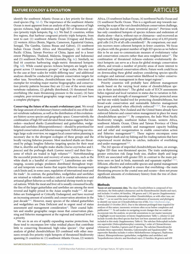
identify the southwest Atlantic Ocean as a key priority for threat-ened species (Fig. 5d–f). The importance of the southwest Atlantic Ocean is most apparent from an analysis of the congruence of high species richness, high endemism and high ED of threatened spe-cies (priority triple hotspots; Fig. 6c). We find 21 countries, within five regions, that harbour congruent priority triple hotspots, from west to east: (1) southwest Atlantic Ocean (Uruguay and Brazil), (2) western Africa (Benin, Nigeria, Cameroon, Equatorial Guinea, Senegal, The Gambia, Guinea Bissau and Gabon), (3) southwest Indian Ocean (South Africa and Mozambique), (4) northwest Pacific (China, Taiwan Province of China, Japan and to a lesser extent Philippines, Thailand, Malaysia, Singapore and Indonesia) and (5) southwest Pacific Ocean (Australia; Fig. 6c). Similarly, we find 44 countries harbouring single-metric threatened hotspots (Fig. 6d). While coastal species richness hotspots are largely con-gruent across 13 taxonomic groups36 at large scales, this may not be the case at finer scales for widely differing taxa37 and additional analyses should be conducted to pinpoint conservation targets for other taxa. Nevertheless, chondrichthyans may be considered an exemplar for revealing major marine biogeographic and conserva-tion priority patterns because they are (1) one of the seven major vertebrate radiations, (2) globally distributed, (3) threatened from overfishing (the main threatening pressure in the ocean), (4) have complete, peer-reviewed geographic range maps and (5) now have a complete phylogeny.

Conserving the future of the ocean’s evolutionary past. We reveal the large amount of evolutionary history embodied in one of the old-est vertebrate radiations, as well as the distribution of this evolution-ary history across species and geographic space. Conservatively, the combination of high ED and elevated threat status suggests that two orders—mackerel sharks (Lamniformes) and guitarfishes, wedge-fishes and sawfishes (Rhinopristiformes)—should be prioritized for targeted conservation and fisheries management. Following our stra-tegic large-scale overview, we suggest local conservation planning is necessary due to the divergent ecologies of these groups and the locally varying fisheries pressure. Most mackerel sharks are threat-ened by pelagic longline fisheries targeting species for their meat (that is, shortfin and longfin mako sharks (Isurus oxyrinchus and I. paucus) and the porbeagle shark (Lamna nasus)) and their fins—some of which are traded in high volumes38,39. Notwithstanding the successful protection and recovery of some species, such as the white shark in a handful of countries40,41, Lamniformes are wide-ranging, oceanic-pelagic predators distributed throughout tropi-cal and temperate ocean basins that require fisheries management catch limits and, in some cases, regulation of international meat and fin trade42. In contrast, the guitarfishes, wedgefishes and sawfishes are retained as valuable secondary catch in coastal subsistence and artisanal gillnet fisheries as well as industrial shrimp trawls in tropi-cal nations. While the meat and liver oil is usually consumed locally, the fins of the larger guitarfishes and sawfishes are among the most revered and highly prized in the Asian soupfin trade39,43. All saw-fishes are Endangered or Critically Endangered, and have received an increasing amount of scientific and conservation attention in the past decade44,45. However, many species of the related guitarfishes and wedgefishes are Data Deficient and in urgent need of status assessment and management consideration46. Their coastal habi-tats and smaller geographic ranges mean that conservation plan-ning and fisheries management at the regional and national level is a priority.

We are in an era of rapidly expanding marine protections, but these tend to encompass low-value residual places that contribute little to conserving threatened, high-value species33. Our spatial analysis of global chondrichthyan ED combined with other mea-sures reveals five priority triple hotspots of threatened biodiversity spanning 21 countries in: (1) southwest Atlantic Ocean, (2) western

Africa, (3) southwest Indian Ocean, (4) northwest Pacific Ocean and (5) southwest Pacific Ocean. This is a significant step towards nar-rowing the scope of the vast chondrichthyan conservation challenge, which far exceeds that of many terrestrial species30. Previous work has only considered hotspots of species richness and endemism of sharks alone—that is, without rays or chimaeras—and recovered an impractically large and geographically diffuse array of 4,103 priority grid cells (14.2% of all cells considered)31. By comparison, our anal-ysis recovers more coherent hotspots in fewer countries. We focus on places with the greatest number of high ED species as we believe this to be an easy-to-communicate measure of evolutionary value and conservation concern rather than area-weighted ratios8,47. The combination of threatened richness–endemic–evolutionarily dis-tinct hotspots can serve as a focus for global strategic conservation efforts, and reveals a number of priority areas of more interest to national and regional conservation efforts. Future work could focus on downscaling these global analyses considering species-specific ecologies and national conservation likelihood to tailor conserva-tion and fisheries management in these target regions33.

Priority countries will probably have different management needs based on the varying local status of chondrichthyan spe-cies in their jurisdictions30. The global scale of IUCN assessments belies regional and local variation in status due to variation in fish-ing pressure and strength of management48. Marine protected areas are but one widely lauded tool for protecting chondrichthyans, but broad-scale conservation and sustainable fisheries management have great potential when effectively enforced40, 42,49. For example, Australia, Canada, New Zealand and the United States already have enforced fisheries and conservation management in place for many chondrichthyan species42,50. By comparison, the Indo-West Pacific biodiversity triangle, southwest Indian Ocean, western Africa, southwest Atlantic Ocean, China and Taiwan Province of China need considerable scientific and management capacity building and aid relief and reorganization to enable conservation action and fisheries management30,33. These regions encompass some of the largest shark and ray fishing and fin-trading nations that have experienced recent declines in catches, indicative of overfishing and under-management19,20.

The 242 species of imperiled chondrichthyans have, on average, higher ED than non-threatened species. The traits underpinning greater extinction risk (large body size, shallow depth and large EOO) are associated with greater ED; in contrast to the main pat-terns seen on land in birds, mammals and squamate reptiles8, 10,12. Efficient, effective and enforceable species and spatial management strategies should be adopted to ensure that overfishing—the main threatening process in the coastal seas and oceans—does not prune significant amounts of evolutionary history from the tree of chon-drichthyan life.

MethodsTaxon set and taxonomic data. The class Chondrichthyes is composed of two subclasses, the Holocephali (chimaeras) and the Elasmobranchii (sharks and rays), and includes 14 orders, 60 families, 198 genera and 1,192 species (Supplementary Table 1). Systematic relationships within Chondrichthyes, as with other taxa, are in flux51–54, so we used the most recent combination of taxonomy and phylogeny to identify our taxon set (Chondrichthyan tree of life, http://sharksrays.org/, downloaded 15 October 2015). Due to the inherent prolonged time required for analyses of this nature, taxonomic revisions often occur before completion and publication55–59. To aid readers in navigating recent changes that we could not incorporate into the analysis, we provide annotations to our master taxonomy to highlight recent taxonomic revisions (Supplementary Table 1, column G) and include recently described species that have not been assessed and could not be included in this study (Supplementary Table 6). The subclass Holocephali includes one superorder (Holocephalimorpha) containing 1 order of Chimaeriformes (chimaeras); 3 families, 6 genera and 49 species. The subclass Elasmobranchii includes three superorders: Batoidea, Galeomorphii and Squalomorphii60. The superorder Batoidea includes 4 orders Myliobatiformes (stingrays), Rajiformes (skates), Rhinopristiformes (guitarfishes, wedgefishes and sawfishes) and Torpediniformes (electric and thornback rays); 23 families, 86 genera and 639


http://sharksrays.org/




species. The sharks comprise two superorders: Galeomorphii and Squalomorphii. The superorder Galeomorphii includes 4 orders: Carcharhiniformes (ground sharks), Heterodontiformes (bullhead sharks), Lamniformes (mackerel sharks) and Orectolobiformes (carpet sharks); 23 families, 75 genera and 347 species. The superorder Squalomorphii includes 5 orders Hexanchiformes (cow sharks), Pristiophoriformes (saw sharks), Echinorhiniformes (bramble sharks), Squaliformes (dogfish sharks) and Squatiniformes (angel sharks); 11 families, 31 genera and 157 species. The taxonomic hierarchy described above comprises the taxonomic data that we used to place and constrain those taxa without DNA sequence data (see Supplementary Table 1 and ‘Taxon-complete trees’ section below).

DNA data matrix. We assembled a DNA data supermatrix from pre-existing GenBank and Barcode of Life Data System records (downloaded on or before 15 September 2014) as well as 54 novel sequences generated for this study. Data from GenBank can present particular challenges, outlined in ref. 51; thus, all sequence and species validity was checked before analysis. Of particular concern with GenBank sequence data is the potential for misidentified specimens leading to erroneous placement. As a check for this, an initial set of trees were generated using RAxML61 and their topology was hand-checked to verify reasonable placement of species included in our matrix. The matrix is composed of a novel set of 15 coding and non-coding regions as follows: 2 non-protein-coding mitochondrial loci (12S and 16S ribosomal DNA, 2,037 bp), 11 protein-coding mitochondrial loci (CO1, CO2, CO3, Cyt b, ND1, ND2, ND3, ND4, ND4L, ND5 and ND6; 10,341 bp) and 2 nuclear protein-coding loci (RAG1, 2,538 bp; SCFD2, 582 bp; Supplementary Table 2). The novel sequence data generated for this study include 8 CO1, 1 Cyt b, 1 ND2, 1 ND4 and 42 RAG1 sequences. The supermatrix included representatives from all 14 orders, 59/60 families (98%), 173/198 genera (88%) and 642 species (645 originally, of which 3 were subsequently synonymized with valid names and removed) out of 1,192 species (54%). At its maximum extent, the DNA data matrix comprises 15,498 bp; however, the alignment is sparse and taxonomic coverage averages 30% across loci (mitochondrial loci: 13–81%; nuclear loci 12–27%; Supplementary Table 2).

We used MAFFT v.7.22162–64 to conduct local alignments for each locus. Nuclear and mitochondrial protein-coding sequences are straightforward to align, but mitochondrial non-protein-coding sequences are subject to high frequencies of insertions and deletions (indels). Therefore, we aligned the indel-rich mitochondrial 12S and 16S non-protein-coding sequences in two stages: first, we aligned the sequences by taxonomic order, and second, we combined the resulting order-specific alignments and realigned the entire set together. We removed start and stop codons from aligned protein-coding sequences before testing nucleotide substitution models. We used JModelTest 2.065,66 and AIC to identify the best-fit nucleotide substitution model for each locus. Three closely related best-fit models were identified: GTR + Γ (nuclear RAG1), GTR + Γ + Ι (mitochondrial 12S, 16S, CO1, CO2, Cyt b, ND1, ND2, ND3, ND4, ND4L, ND5 and ND6) and SYM + Γ + Ι (mitochondrial CO3 and nuclear SCFD2). Invariant site models, such as GTR + Γ + Ι and SYM + Γ + Ι , have been criticized because the proportion of invariant sites and the gamma shape parameter cannot be optimized independently. As a consequence, it is impossible to obtain reliable estimates for these parameters simultaneously67. The SYM model is a constrained, nested version of the GTR model.

We used RAxML61 to infer individual gene trees and species trees based on partitioned, concatenated analyses. RAxML uses a computationally efficient version of GTR (GTRCAT) that accommodates rate heterogeneity and GTRCAT is a good fit for our small set of best-fit models. In the final step, the GTRCAT model optimizes parameters and calculates likelihood under GTR + Γ 61. We conducted 1,000 bootstrap replicates in each analysis and inspected the resulting topologies for consistency and bootstrap support before proceeding with partitioned, concatenated analyses. We used a pragmatic and iterative approach to partitioning, which was informed by constraints on a small, sparse dataset and trade-offs associated with variation in nucleotide substitution rate and process. Nuclear sequences typically evolve slowly relative to mitochondrial sequences, and the two nuclear protein-coding sequences (RAG1 and SCFD2) were assigned to separate partitions. Although the mitochondrion is inherited as a single locus, its protein-coding and non-protein-coding sequences exhibit different nucleotide substitution rates and indel frequencies. As a consequence, mitochondrial non-protein-coding and protein-coding loci were assigned to two separate partitions. Mitochondrial protein-coding sequences are subject to codon-position-specific rate variation. One consequence of this rate variation is that the faster-evolving mitochondrial third-codon position nucleotides (M3CPN) can become saturated over long periods of evolutionary time, and there is precedence for excluding M3CPN from phylogenetic reconstructions for ancient clades68,69. As part of our iterative approach to partitioning, we first conducted RAsML analyses with 1,000 bootstrap replicates and then used RogueNaRok (http://rnr.h-its.org/)70 to identify rogue taxa that erode bootstrap support. In RogueNaRok analyses, we specified the parameters as follows: threshold: 50% majority rule consensus; optimize: support; and max drop set: 3. In addition, we employed a raw-improvement-score threshold (0.5), which corresponds to a relatively large improvement of overall support, to identify and exclude rogue taxa70.

When we excluded the M3CPN, RAsML analyses generated trees with low-overall bootstrap support, and two iterations of rogue identification yielded 60 rogue taxa (9.3%). Despite concerns over saturation, we tried including the M3CPN in a standard, uniform block alignment. This resulted in a substantial increase in overall bootstrap support, and two iterations of rogue identification yielded just 22 rogue taxa (3.4%). However, bootstrap support remained low at relatively deep nodes (among orders and among families within orders) within the superorder Batoidea. Batoidea comprises 4 orders and 23 families: Myliobatiformes (10 families), Rajiformes (3 families), Rhinopristiformes (5 families) and Torpediniformes (5 families). As a consequence, the impact of low bootstrap support on topology is large. In an attempt to reduce the potential negative impacts of saturation and generate increased bootstrap support for the deeper nodes within Batoidea, we implemented a novel, staggered-by-order alignment approach for the M3CPN. Instead of using a single uniform block alignment, we extracted all of the M3CPN and placed them in a separate partition. This resulted in two partitions for the mitochondrial protein-coding loci, one with first- and second-codon position nucleotides and another with third-codon position nucleotides. The partition containing first- and second-codon position nucleotides remained as a standard uniform block alignment. For the partition containing the third-codon position nucleotides, we staggered the alignment by taxonomic order. The consequence of this novel partitioning/alignment approach is that the M3CPN sequence data can only speak to affinities within, but not between, orders. This approach resulted in increased bootstrap support within Batoidea without loss of support in other parts of the phylogeny. Two iterations of rogue identification yielded 21 rogue taxa (3.3%). Importantly, 11 taxa, including the worst offenders in both analyses including M3CPN, were included in the shared subset of rogue taxa. Using the staggered-by-order approach for the M3CPN alignment and two iterations of rogue identification, we identified and excluded 21 rogue taxa from 15 genera: Bathyraja (n = 2), Carcharhinus (2), Centrophorus, Dipturus (2), Discopyge, Isogomphodon, Leptocharias, Mustelus, Narke (2), Orectolobus, Potamotrygon (3), Raja, Spiniraja, Squalus and Squatina (Supplementary Table 1). There were still many nodes with bootstrap support < 70% and these were collapsed before incorporating unresolved taxa, when the identified rogue taxa were also reintroduced. This means that there was likely very little effect of rogue selection on overall topology. While the novel staggered-by-order approach employed here with the M3CPN partition appears promising, it warrants further study.

Temporal calibration. Ideally, calibration fossils should be subjected to a formal phylogenetic analysis or exhibit diagnostic apomorphies71; unfortunately, relatively few fossils assigned to Chondrichthyes meet these criteria72. There are three exceptions: (1) Chondrenchelys problematicus, which has affinities with stem Holocephalii (Chimaeriformes)73, (2) Tingitanius tenuimandibulus, which has affinities with stem Platyrhinidae (thornback rays)74, and (3) Protospinax annectans, which has affinities with the stem of the superorder Squalomorphii, a clade including Hexanchiformes, Pristiophoriformes, Squaliformes and Squatiniformes75. We identified seven additional calibration fossils that are distributed across the Chondrichthyan phylogeny; several of these are represented by substantial articulated remains (Supplementary Table 3). Chondrenchelys problematicus is the only formally vetted calibration fossil and, importantly, it provides a hard minimum bound for the chondrichthyan root node (333.56 Myr)72. The root node of Chondrichthyes is further characterized by a soft maximum bound of 422.4 Myr (see ref. 72 for justification). Following Ho and Phillips76, we used these hard minimum and soft maximum bounds to specify a lognormal calibration density and selected a mean that bounded 95% of the probability density within the 88.84 Myr interval between the hard minimum and soft maximum bounds and a standard deviation that split the probability density evenly across the midpoint (377.98 Myr) of this interval. While the ages of the nine other calibration fossils provide hard minimum bounds for their calibrated nodes, there is not sufficient information to generate a calibration density for any of them.

We used ‘treePL’ 1.0 in Ubuntu 14.0477, which implements a flexible rate-smoothing algorithm, to assign a timeline of diversification to the phylogeny. Given the rate-smoothing behaviour of ‘treePL’ and the reported low substitution rate in chimaeras78, we expect the actual crown age of Chimaeriformes to be older, and the Elasmobranchii crown age to be younger, than reported here. Given uncertainty in the precise phylogenetic affinities of at least seven of the nine additional fossils, we chose to conduct two sets of dating analyses, one that included Chondrenchelys problematicus only, and another that included all ten calibration fossils (Supplementary Table 3). For both of these calibration scenarios, we generated a random sample of 500 root-node ages from the lognormal calibration density that we constructed for the root node (together measuring the root age we report), and then conducted separate ‘treePL’ analyses using each of the 500 root-node ages. Our ‘treePL’ analyses proceeded in two stages. In the first, we performed cross-validation analyses (‘cv’ and ‘randomcv’ commands) and tested performance of the available optimization routines (‘prime’ command). In the second, we incorporated control options (‘thorough’ command) to ensure that the preferred optimization routine converged. The 500 resulting ‘treePL’-dated topologies for each of the two calibration scenarios were subsequently used in the taxon-complete analyses described below. Importantly, the topology recovered from our RAxML analyses of the concatenated data matrix, remained fixed across all of these ‘treePL’ analyses;


http://rnr.h-its.org/




only the timeline of diversification changed between the two calibration scenarios and across the 500 root-node ages. The ‘treePL’ output was converted into a single 500-tree Newick file, processed with TreeAnnotator 1.7.579 using the default settings (no burn-in; posterior probability limit 0.0; maximum clade credibility tree; median node heights).

Taxon-complete trees. We added taxa without DNA sequence data to each of the 500 ‘treePL’-dated, molecular trees (‘stage 1’ trees) and then used a taxon-addition and polytomy-resolver algorithm (modified from ref. 22; details below) to generate a large distribution of fully resolved, taxon-complete candidate phylogenies. We used two taxonomic sources: the Chondrichthyan tree of life (http://sharksrays.org) and the IUCN Red List (http://www.iucnredlist.org). Our distribution of taxon-complete trees includes three types of species80. Type 1 species have genetic data and are represented in the stage 1 trees. Type 2 species have no genetic data (or were identified as rogue taxa), but have at least one congener represented in the stage 1 trees. Type 3 species have no genetic data (or were identified as rogue taxa), and have no congeners in the stage 1 trees. Type 2 and type 3 species were allowed to populate particular clades using taxonomic information and the topology (via node identities) of the stage 1 trees. We outline the rules we used to include taxa without any sequence data below.

Type 1 species were anchored relative to one another as resolved in the stage 1 trees, and we used 70% bootstrap-support (BS) as a threshold to topologically constrain inferred nodes during taxon addition. There were four scenarios in which the stage 1 trees needed to be modified to enforce genus, family or order monophyly (Supplementary Table 4).

• First, there were nine genera with relatively weak support (BS < 70%; range: 7–68%) for genus monophyly within a highly supported clade (BS ≥ 70%; Sup-plementary Table 4). For these nine genera instances, we pruned ten type 1 taxa from the stage 1 trees, reducing its size from 620 to 610 species. We reincor-porated these ten pruned taxa subsequently as type 2 species by constraining them to their named clades.

• Second, there were four families (Anacanthobatidae, Hemigaliidae, Somniosi-dae and Triakidae) where there was weak support (BS < 70%; range: 33–62%) for family non-monophyly. In these four instances, we collapsed the weakly supported nodes and subsequently reconstituted clades to enforce family monophyly80 (Supplementary Table 4).

• Third, there were 24 mixed-genus and/or mixed-family clades with strong evidence (BS ≥ 70%) against monophyly for at least one genus or family. These ‘mixed clades’ took on a variety of forms, from simple paraphyly to complex interdigitation of sub-genera or sub-families. We enforced genus monophyly for any genus or family within these mixed clades, unless there was strong evidence (BS ≥ 70%) against monophyly.

• Finally, for consistency between taxa with and without genetic data, we assumed that all genera, families and orders were monophyletic unless there was strong evidence (BS ≥ 70%) against monophyly in the stage 1 trees. This rule affected one subgenus (Galeus minor clade), nine genera (Atlantoraja, Centrophorus, Chiloscyllium, Halaelurus, Mobula, Rajella, Rhinobatos, Sphyrna and Squalus), one mixed-genus clade (Dentiraja, Dipturus, Spiniraja together with Zearaja), one family (Pristidae) and one order (Orectolobiformes) in our stage 1 trees—each of these had only weak evidence (BS < 70%; range 32-69%) for monophyly.

After using these rules to modify the stage 1 trees, we imposed topological constraints on the placement of the remaining type 2 and type 3 species, including the 21 rogue taxa. Each type 2 species was restricted to its genus or its mixed-genus clade. There were four genera (Dasyatis, Galeus, Himantura and Triakis) with strong evidence (BS ≥ 70%) against monophyly in the stage 1 trees that also required the addition of type 2 species. For these four genera, type 2 congeners were added to the largest candidate sub-clade for the genus. Each type 3 species was restricted to its named genus, and the entire genus was constrained in its placement among other genera according to higher-level (supergenus, family or order) taxonomic information (Supplementary Table 1). Of the 198 recognized genera, 23 were not represented in the stage 1 trees, and these 23 genera were restricted to 6 of the 14 orders and 18 of the 60 families (Supplementary Table 1). There were 9 type 3 species not assigned to a family on http://sharksrays.org/. In these instances, we referred to the IUCN (https://www.iucn.org/) for the original family-level designation (Supplementary Table 1).

The 500 dated taxon-complete trees were then each resolved using Polytomy Resolver22, modified to allow for the partial constraints enumerated above. The Polytomy Resolver algorithm uses a customized R-script to generate an input file for BEAST 1.x, based on the original dated phylogeny, and the taxonomy additions outlined above. The generated input file leverages BEAST’s ability for ‘prior only sampling’, combined with a series of hierarchical topology constraints—both time-based and monophyly-based—that define the original tree topology and allowable taxon additions, to sample taxon-complete trees across tree-space. For both fossil calibration scenarios, mean growth rate (birth–death) was unconstrained, while we set uniform flat priors for relative death rate (death/birth; one fossil calibration: 0.4–0.85; ten fossil calibration: 0.25–0.75). Each taxon infilling scenario was run

in BEAST 1.7.579 for three million generations including a one million generation burn-in. Samples were drawn every 100,000 generations to avoid temporal autocorrelation between draws, and the resulting 20 trees from each of 500 scenarios were collated into a pseudo-posterior distribution of 10,000 fully resolved trees. Trees are available for download via http://www.sharktree.org.

Evolutionary distinctness. Evolutionary isolation metrics rank species by the amount of ancestry shared with relatives. We used the ED measure first presented by Redding21, which sums the lengths of the branches on the path from a species to the root, with each branch inversely weighted by the number of species that it subtends: species with longer branches on the path leading to the root of the tree, and with fewer relatives that share these branches have higher ED scores. As intuited by Hartmann81, and shown formally by Fuchs and Jin82, ED is formally equivalent to the Shapley index83 on rooted trees84. Importantly, the sum of the ED values across all tips equals the total evolutionary history of the tree. Given this, for Fig. 2, we calculated the expected ED per species for each major vertebrate lineage using species richness and crown age and the method of moments estimator of diversification rate85. When calculating the expected total tree length of a birth–death tree from theorem 4 of Mooers et al.86, setting extinction rate = 0.75 × speciation rate produced the best global fit to the true average ED scores for birds, mammals, amphibians, squamate reptiles and chondrichthyans. Input data and references can be found in Supplementary Table 5. When measured on the same scale (for example, millions of years for time-calibrated trees), ED scores are broadly comparable across large taxonomic groups87. ED is also the metric currently used by the Zoological Society of London to rank species for its EDGE programme (http://www.edgeofexistence.org).

Extinction risk assessment and estimation. We used the IUCN Red List categories and criteria26 to assign relative extinction risk. The IUCN Shark Specialist Group categorized 604 of 1192 taxonomically valid species into one of five categories: Critically Endangered (CR), Endangered (EN), Vulnerable (VU), Near Threatened (NT) and Least Concern (LC). In addition, there was 588 species that were either categorized as Data Deficient (n = 477) or recognized on http://sharksrays.org/ that are Not Evaluated by the IUCN Shark Specialist Group (n = 111). We categorized these species as threatened or otherwise based on a generalized linear model with binomial error and logit link and three traits: body size (cm, total length), upper depth limit (m) and depth range (m). These models have good predictive power (area under the curve = 0.77). To test for relationships among candidate covariates of threat and ED, we compared our three traits (body size, depth and EOO (as a measure of range size) across all chondrichthyan species and subsets of Elasmobranchii (sharks and rays) using a general linear modelling framework. Before testing, all traits and median estimates of species-specific ED were log10 transformed. Prediction intervals were generated across the full range of each trait holding the others to their median value. Tests of covariation were repeated using phylogenetic generalized least squares to account for non-independence of species using caper version 0.5.288. To account for uncertainty in the topology, phylogenetic generalized least squares analyses were performed on 100 trees randomly sampled from the posterior tree distribution. Means values of parameter estimates, standard errors, AIC and phylogenetic signal λ are reported in the Supplementary Results.

Spatial analysis. We used the EOO maps from the IUCN Red List available in December 201527. Geographic distributions (EOO) were not available for 111 species; hence only 1,081 of the 1,192 species were included in the spatial analysis. A key advantage of our approach is the use of the IUCN EOO maps, which are compiled and peer-reviewed by experts. The final maps are created using a minimum convex polygon around all location records accounting for the distribution of scientific collection and survey effort. Using point locality data, such as location records from the Global Biodiversity Information Facility (https://www.gbif.org), are known to have spatial and species bias, that is, towards higher gross domestic product countries and commercially valuable species, and contain omission errors (a species is not present, when in fact it is)89. Although EOO maps are known to create commission errors (a species is mapped to be present in an area when in fact it is not), commission rather than omission errors are preferred89,90.

We created a global hexagonal grid of 23,322 km2 cells91,92. We define threatened species as those in the IUCN Red List categories Critically Endangered, Endangered or Vulnerable, but we also included those 50 species with both an EOO map and predicted to be threatened. Together we refer to this combination of threatened and that are predicted to be threatened species as the imperiled species set. We define a species as endemic based on the median EOO range size (419,932 km2; n = 541)93,94. We used this definition previously, but the value of the median used here differs slightly (595,749 km2, n = 504) due to addition of species to the IUCN database and the inclusion of freshwater species19. We defined top 25% ED as those species within the highest quartile of mean ED scores and present the number of species per cell within the upper quartile ED.

To determine hotspots, we used R version 3.2.495 with package plyr version 1.8.396, sp version 1.2-297 and ArcGIS version 10.398. Smoothing was completed for visual clarity purposes only. Hotspots, however, were not smoothed to preserve the accuracy of the locations. Hotspot cells were assigned to countries based on


http://sharksrays.org

http://sharksrays.org

http://www.redlist.org


http://iucn.org/

http://www.sharktree.org

http://www.EdgeofExistence.org


http://data.gbif.org

http://data.gbif.org




whether the cell, regardless of how much, overlapped with a country’s exclusive economic zone99. Regional analyses will need to be completed to more accurately assign hotspot responsibility to these countries.

Life Sciences Reporting Summary. Further information on experimental design is available in the Life Sciences Reporting Summary.

Data availability. The authors declare that all data supporting the findings of this study are available within the paper and its Supplementary Information files. In addition, phylogenetic trees generated during this study are accessible via http://www.sharktree.org.

Received: 1 December 2016; Accepted: 8 December 2017; Published: xx xx xxxx

References 1. Wilson, K. A., McBride, M. F., Bode, M. & Possingham, H. P. Prioritizing

global conservation efforts. Nature 440, 337–340 (2006). 2. Bottrill, M. C. et al. Is conservation triage just smart decision making? Trends

Ecol. Evol. 23, 649–654 (2008). 3. Waldron, A. et al. Targeting global conservation funding to limit immediate

biodiversity declines. Proc. Natl. Acad. Sci. USA 110, 1–5 (2013). 4. Andelman, S. J. & Fagan, W. F. Umbrellas and flagships: efficient conservation

surrogates or expensive mistakes? Proc. Natl. Acad. Sci. USA 97, 5954–5959 (2000).

5. Faith, D. P. Conservation evaluation and phylogenetic diversity. Biol. Conserv. 61, 1–10 (1992).

6. Faith, D. P. in The Routledge Handbook of Philosophy of Biodiversity (eds Garson, J., Plutynski, A. & Sarkar, S.) 69-85 (Routledge, New York, NY, 2017).

7. Vane-Wright, R. I., Humphries, C. J. & Williams, P. H. What to protect? Systematics and the agony of choice. Biol. Conserv. 55, 235–254 (1991).

8. Jetz, W. et al. Global distribution and conservation of evolutionary distinctness in birds. Curr. Biol. 24, 919–930 (2014).

9. Stuart, S. N., Wilson, E. O., McNeely, J. A., Mittermeier, R. A. & Rodríguez, J. P. The barometer of life. Science 328, 177 (2010).

10. Isaac, N. J. B., Turvey, S. T., Collen, B., Waterman, C. & Baillie, J. E. M. Mammals on the EDGE: conservation priorities based on threat and phylogeny. PLoS. ONE 2, e296 (2007).

11. Isaac, N. J. B., Redding, D. W., Meredith, H. M. & Safi, K. Phylogenetically-informed priorities for amphibian conservation. PLoS. ONE 7, 1–8 (2012).

12. Tonini, J. F. R., Beard, K. H., Ferreira, R. B., Jetz, W. & Pyron, R. A. Fully-sampled phylogenies of squamates reveal evolutionary patterns in threat status. Biol. Conserv. 204 (Part A), 23–31 (2016).

13. Heupel, M. R., Knip, D. M., Simpfendorfer, C. A. & Dulvy, N. K. Sizing up the ecological role of sharks as predators. Mar. Ecol. Prog. Ser. 495, 291–298 (2014).

14. Hussey, N. E. et al. Expanded trophic complexity among large sharks. Food Webs 4, 1–7 (2015).

15. Burkholder, D. A., Heithaus, M. R., Fourqurean, J. W., Wirsing, A. & Dill, L. M. Patterns of top-down control in a seagrass ecosystem: Could a roving apex predator induce a behaviour-mediated trophic cascade? J. Anim. Ecol. 82, 1192–1202 (2013).

16. Ruppert, J. L. W., Travers, M. J., Smith, L. L., Fortin, M. J. & Meekan, M. G. Caught in the middle: combined impacts of shark removal and coral loss on the fish communities of coral reefs. PLoS. ONE 8, 1–9 (2013).

17. Mull, C. G., Yopak, K. E. & Dulvy, N. K. Does more maternal investment mean a larger brain? Evolutionary relationships between reproductive mode and brain size in chondrichthyans. Mar. Freshw. Res. 62, 567–575 (2011).

18. Dulvy, N. K. & Reynolds, J. D. Evolutionary transitions among egg− laying, live− bearing and maternal inputs in sharks and rays. Proc. R. Soc. B Biol. Sci. 264, 1309–1315 (1997).

19. Davidson, L. N. K., Krawchuk, M. A. & Dulvy, N. K. Why have global shark and ray landings declined: Improved management or overfishing? Fish Fish 17, 438–458 (2016).

20. Dulvy, N. K. et al. Extinction risk and conservation of the world’s sharks and rays. eLife 3, e00590 (2014).

21. Redding, D. W. Incorporating Genetic Distinctness and Reserve Occupancy into a Cconservation Prioritisation Approach. MSc Thesis, Univ. East Anglia (2003).

22. Kuhn, T. S., Mooers, A. & Thomas, G. H. A simple polytomy resolver for dated phylogenies. Methods Ecol. Evol. 2, 427–436 (2011).

23. Thomas, G. H. et al. PASTIS: an R package to facilitate phylogenetic assembly with soft taxonomic inferences. Methods Ecol. Evol. 4, 1011–1017 (2013).

24. McClenachan, L., Cooper, A. B., Carpenter, K. E. & Dulvy, N. K. Extinction risk and bottlenecks in the conservation of charismatic marine species. Conserv. Lett. 5, 73–80 (2012).

25. Maxwell, S. L., Fuller, R. A., Brooks, T. M. & Watson, J. E. M. The ravages of guns, nets and bulldozers. Nature 536, 143–145 (2016).

26. Mace, G. M. et al. Quantification of extinction risk: IUCN’s system for classifying threatened species. Conserv. Biol. 22, 1424–1442 (2008).

27. IUCN The IUCN Red List of Threatened Species Version 2014.1 (IUCN, 2014). 28. Verde Arregoitia, L. D., Blomberg, S. P. & Fisher, D. O. Phylogenetic

correlates of extinction risk in mammals: species in older lineages are not at greater risk. Proc. Biol. Sci. 280, 20131092 (2013).

29. Field, I. C., Meekan, M. G., Buckworth, R. C. & Bradshaw, C. J. A. Susceptibility of sharks, rays and chimaeras to global extinction. Adv. Mar. Biol. 56, 275–363 (2009).

30. Dulvy, N. K. et al. Challeneges and priorities in shark and ray conservation. Curr. Biol. 27, R565–R572 (2017).

31. Lucifora, L. O., García, V. B. & Worm, B. Global diversity hotspots and conservation priorities for sharks. PLoS. ONE 6, e19356 (2011).

32. Trebilco, R. et al. Mapping species richness and human impact drivers to inform global pelagic conservation prioritisation. Biol. Conserv. 144, 1758–1766 (2011).

33. Davidson, L. N. K. & Dulvy, N. K. Global marine protected areas to prevent extinctions. Nat. Ecol. Evol. 1, 0040 (2017).

34. Rosauer, D. F. & Mooers, A. O. Nurturing the use of evolutionary diversity in nature conservation. Trends Ecol. Evol. 28, 322–323 (2013).

35. Lennon, J. J., Koleff, P., Greenwood, J. J. D. & Gaston, K. J. Contribution of rarity and commonness to patterns of species richness. Ecol. Lett. 7, 81–87 (2004).

36. Tittensor, D. P. et al. Global patterns and predictors of marine biodiversity across taxa. Nature 466, 1098–1101 (2010).

37. Orme, C. D. L. et al. Global hotspots of species richness are not congruent with endemism or threat. Nature 436, 1016–1019 (2005).

38. Clarke, S. C. et al. Global estimates of shark catches using trade records from commercial markets. Ecol. Lett. 9, 1115–1126 (2006).

39. McClenachan, L., Cooper, A. B. & Dulvy, N. K. Rethinking trade-driven extinction risk in marine and terrestrial megafauna. Curr. Biol. 26, 1–7 (2016).

40. Curtis, T. H. et al. Seasonal distribution and historic trends in abundance of white sharks, Carcharodon carcharias, in the western North Atlantic Ocean. PLoS. ONE 9, e99240 (2014).

41. Lowe, C. G. et al. in Global Perspectives on the Biology and Life History of the White Shark (ed. Domeier, M.) 169–186 (CRC Press, Boca Raton, FL 2012).

42. Simpfendorfer, C. A. & Dulvy, N. K. Bright spots of sustainable shark fishing. Curr. Biol. 27, R97–R98 (2017).

43. Giles, J., Riginos, C., Naylor, G., Dharmadi & Ovenden, J. Genetic and phenotypic diversity in the wedgefish Rhynchobatus australiae, a threatened ray of high value in the shark fin trade. Mar. Ecol. Prog. Ser. 548, 165–180 (2016).

44. Devitt, K. R., Adams, V. M. & Kyne, P. M. Australia’s protected area network fails to adequately protect the world’s most threatened marine fishes. Glob. Ecol. Conserv. 3, 401–411 (2015).

45. Dulvy, N. K. et al. Ghosts of the coast: global extinction risk and conservation of sawfishes. Aquat. Conserv. Mar. Freshw. Ecosyst. 26, 134–153 (2016).

46. Moore, A. Guitarfishes: the next sawfishes? Extinction vulnerabilites and an urgent call for conservaion action.Endanger. Species Res. 34, 75–88 (2017).

47. Davies, T. J. & Buckley, L. B. Phylogenetic diversity as a window into the evolutionary and biogeographic histories of present-day richness gradients for mammals. Philos. Trans. R. Soc. B Biol. Sci. 366, 2414–2425 (2011).

48. Fernandes, P. et al. Fisheries conservation reveals regional divergence in Europe’s marine fish risk.Nat. Ecol. Evol. 1, 0170 (2017).

49. Peterson, C. D. et al. Preliminary recovery of coastal sharks in the south-east United States.Fish. Fish. 18, 845–859 (2017).

50. White, W. T. & Kyne, P. M. The status of chondrichthyan conservation in the Indo-Australasian region. J. Fish. Biol. 76, 2090–2117 (2010).

51. Naylor, G. J. P. et al. in The Biology of Sharks and Their Relatives (eds Carrier, J. C., Musick, J. A. & Heithaus, M. R.) 31–56 (CRC Press, Boca Raton, FL, 2012).

52. Naylor, G. J. P. et al. A DNA sequence-based approach to the identification of shark and ray species and its implications for globa elasmobranch diversity and parasitology. Bull. Am. Mus. Nat. Hist. 367, 1–262 (2012).

53. Naylor, G. J. P., Ryburn, J. A., Fedrigo, O. & López, J. A. in Reproductive Biology and Phylogeny of Chondrichthyes: Sharks, Batoids, and Chimaeras (eds Hamlett, W. C. & Jamieson, B. G.) 1–25 (CRC Press, Boca Raton, FL, 2005).

54. White, W. T. & Last, P. R. A review of the taxonomy of chondrichthyan fishes: a modern perspective. J. Fish. Biol. 80, 901–917 (2012).

55. Last, P. R. et al. Rays of the World (CSIRO Publishing, Clayton South, 2016). 56. Last, P. R. et al. in Rays of the World, Supplementary Information 1–10

(CSIRO Publishing, Clayton South, 2016). 57. Last, P. R., Weigmann, S. & Yang, L. in Rays of the World, Supplementary

Information 11–34 (CSIRO Publishing, Clayton South, 2016). 58. Weigmann, S. Annotated checklist of the living sharks, batoids and chimaeras

(Chondrichthyes) of the world, with a focus on biogeographical diversity. J. Fish. Biol. 88, 837–1037 (2016).







59. Weigmann, S. Reply to Borsa (2017): comment on ‘Annotated checklist of the living sharks, batoids and chimaeras (Chondrichthyes) of the world, with a focus on biogeographical diversity by Weigmann (2016)’. J. Fish. Biol. 88, 837–1037 (2017).

60. Ebert, D. A., Fowler, S. L. & Compagno, L. J. V. Sharks of the World: A Fully Illustrated Guide (Wild Nature Press, Plymouth, 2013).

61. Stamatakis, A. RAxML-VI-HPC: maximum likelihood-based phylogenetic analyses with thousands of taxa and mixed models. Bioinformatics 22, 2688–2690 (2006).

62. Katoh, K., Kuma, K. I., Toh, H. & Miyata, T. MAFFT version 5: improvement in accuracy of multiple sequence alignment. Nucleic Acids Res. 33, 511–518 (2005).

63. Katoh, K. & Toh, H. Recent developments in the MAFFT multiple sequence alignment program. Brief. Bioinform. 9, 286–298 (2008).

64. Katoh, K., Misawa, K., Kuma, K. & Miyata, T. MAFFT: a novel method for rapid multiple sequence alignment based on fast Fourier transform. Nucleic Acids Res. 30, 3059–3066 (2002).

65. Darriba, D., Taboada, G. L., Doallo, R. & Posada, D. jModelTest 2: more models, new heuristics and parallel computing. Nat. Methods 9, 772–772 (2012).

66. Guindon, S. & Gascuel, O. A simple, fast, and accurate algorithm to estimate large phylogenies by maximum likelihood. Syst. Biol. 52, 696–704 (2003).

67. Yang, Z. Computational Molecular Evolution (Oxford Univ. Press, Oxford, 2006).

68. Inoue, J. G. et al. Evolutionary origin and phylogeny of the modern holocephalans (Chondrichthyes: Chimaeriformes): a mitogenomic perspective. Mol. Biol. Evol. 27, 2576–2586 (2010).

69. Aschliman, N. C. et al. Body plan convergence in the evolution of skates and rays (Chondrichthyes: Batoidea). Mol. Phylogenet. Evol. 63, 28–42 (2012).

70. Aberer, A. J., Krompass, D. & Stamatakis, A. Pruning rogue taxa improves phylogenetic accuracy: an efficient algorithm and webservice. Syst. Biol. 62, 162–166 (2013).

71. Parham, J. F. et al. Best practices for justifying fossil calibrations. Syst. Biol. 61, 346–359 (2012).

72. Benton, M. J. et al. Constraints on the timescale of animal evolutionary history. Palaeontol. Electron. 18, 1–107 (2015).

73. Lund, R. & Grogan, E. D. Relationships of the Chimaeriformes and the basal radiation of the Chondrichthyes. Rev. Fish. Biol. Fish. 7, 65–123 (1997).

74. Claeson, K. M., Underwood, C. J. & Ward, D. J. Tingitanius tenuimandibulus, a new platyrhinid batoid from the Turonian (Cretaceous) of Morocco and the cretaceous radiation of the Platyrhinidae. J. Vertebr. Paleontol. 33, 1019–1036 (2013).

75. Carvalho, M. R. De & Maisey, J. G. Phylogenetic relationships of the Late Jurassic shark Protospinax WOODWARD 1919 (Chondrichthyes: Elasmobranchii). Syst. Paleoecol. 7, 9–46 (1996).

76. Ho, S. Y. W. & Phillips, M. J. Accounting for calibration uncertainty in phylogenetic estimation of evolutionary divergence times. Syst. Biol. 58, 367–380 (2009).

77. Smith, S. A. & O’Meara, B. C. TreePL: divergence time estimation using penalized likelihood for large phylogenies. Bioinformatics 28, 2689–2690 (2012).

78. Venkatesh, B. et al. Elephant shark genome provides unique insights into gnathostome evolution. Nature 505, 174–179 (2014).

79. Drummond, A. J., Suchard, M. A., Xie, D. & Rambaut, A. Bayesian phylogenetics with BEAUti and the BEAST 1.7. Mol. Biol. Evol. 29, 1969–1973 (2012).

80. Jetz, W., Thomas, G. H., Joy, J. B., Hartmann, K. & Mooers, A. O. The global diversity of birds in space and time. Nature 491, 444–448 (2012).

81. Hartmann, K. The equivalence of two phylogenetic biodiversity measures: the Shapley value and fair proportion index. J. Math. Biol. 67, 1163–1170 (2013).

82. Fuchs, M. & Jin, E. Y. Equality of Shapley value and fair proportion index in phylogenetic trees. J. Math. Biol. 71, 1133–1147 (2015).

83. Shapley, L. S. A value for n-person games. Ann. Math. Stud. 28, 307–318 (1953).

84. Haake, C.-J., Kashiwada, A. & Su, F. E. The Shapley value of phylogenetic trees. J. Math. Biol. 56, 479–497 (2008).

85. Magallón, S. & Sanderson, M. J. Absolute diversification rates in angiosperm clades. Evolution 55, 1762–1780 (2001).

86. Mooers, A., Gascuel, O., Stadler, T., Li, H. & Steel, M. Branch lengths on birth-death trees and the expected loss of phylogenetic diversity. Syst. Biol. 61, 195–203 (2012).

87. Redding, D. W., Mazel, F. & Mooers, A. Measuring evolutionary isolation for conservation. PLoS. ONE 9, 1–15 (2014).

88. Orme, D. et al. caper: comparative analysis of phylogenetics and evolution in R (2012).

89. Rondinini, C., Wilson, K. A., Boitani, L., Grantham, H. & Possingham, H. P. Tradeoffs of different types of species occurrence data for use in systematic conservation planning. Ecol. Lett. 9, 1136–1145 (2006).

90. Rodrigues, A. S. L. Improving coarse species distribution data for conservation planning in biodiversity-rich, data-poor, regions: no easy shortcuts. Anim. Conserv. 14, 108–110 (2011).

91. Jenness Enterprises Repeating shapes for ArcGIS (Jenness Enterprises, 2012). 92. Hoffmann, M. et al. The impact of conservation on the status of the world’s

vertebrates. Science 330, 1503–1509 (2010). 93. Pompa, S., Ehrlich, P. R. & Ceballos, G. Global distribution and conservation

of marine mammals. Proc. Natl. Acad. Sci. USA 108, 13600–13605 (2011). 94. Davidson, A. D. et al. Drivers and hotspots of extinction risk in marine

mammals. Proc. Natl. Acad. Sci. USA 109, 3395–3400 (2012). 95. R Core Team R: a language and environment for statistical computing (R

Foundation for Statistical Computing, 2013). 96. Wickham, H. The split–apply–combine strategy for data. J. Stat. Softw. 40,

1–29 (2011). 97. Pebesma, E. J. & Bivand, R. S. Classes and method for spatial data in R. R.

News 5, 9–13 (2005). 98. ESRI ArcGIS (ESRI, 2011). 99. VLIZ World EEZ v7 (VLIZ, 2014).

AcknowledgementsWe are grateful to A. J. Aberer for useful discussion of rogue taxon exclusion, D. Ebert and W. White for taxonomic guidance, G. J. P. Naylor, X. Vélez-Zauzo, A. Godknecht, M. Gollock, H. Koldewey and M. D’Angelo for research support, and B. Corrie and M. Siegert for computing access. We thank all IUCN Shark Specialist Group members and all additional experts who have contributed data and their expertise to IUCN Red List assessments. This work was carried out at the Interdisciplinary Research in Mathematics and Computer Sciences Centre, Simon Fraser University (http://www.irmacs.sfu.ca), the Swiss Shark Foundation computing cluster and Compute Canada’s Westgrid computing network. This study was funded by Save Our Seas Foundation, Rufford Foundation, Zoological Society London, Natural Science and Engineering Research Council Discovery and Accelerator Awards, and Canada Research Chairs Program. Shark and ray silhouettes in Figs. 1, 2 and 4 were created by C.G.M from images by R. Aidan Martin; all silhouettes in Fig. 3 were created by M. Dando.

Author contributionsN.K.D. and A.O.M. conceived and led the project, R.W.S., C.G.M., J.B.J., T.S.K., N.C.A., L.N.K.D. and A.O.M. designed the project. N.C.A., R.W.S., C.G.M., J.B.J., G.J.S. and L.N.K.D. acquired or provided data. R.W.S., T.S.K., J.B.J. and L.N.K.D. contributed essential code and analyses. R.W.S., C.G.M., L.N.K.D., N.K.D. and A.O.M. drafted and revised the paper. R.W.S. designed and led the phylogenetic work, C.G.M. supported the phylogenetic work and led the subsequent statistical analyses, and L.N.K.D. led the spatial analyses.

Competing interestsThe authors declare no competing financial interests.

Additional informationSupplementary information is available for this paper at https://doi.org/10.1038/s41559-017-0448-4.

Reprints and permissions information is available at www.nature.com/reprints.

Correspondence and requests for materials should be addressed to C.G.M. or N.K.D. or A.O.M.

Publisher’s note: Springer Nature remains neutral with regard to jurisdictional claims in published maps and institutional affiliations.


http://www.irmacs.sfu.ca

http://www.irmacs.sfu.ca

https://doi.org/10.1038/s41559-017-0448-4

https://doi.org/10.1038/s41559-017-0448-4

http://www.nature.com/reprints


1

nature research | life sciences reporting summ

aryJune 2017

Corresponding author(s): Christopher Mull

Initial submission Revised version Final submission

Life Sciences Reporting SummaryNature Research wishes to improve the reproducibility of the work that we publish. This form is intended for publication with all accepted life science papers and provides structure for consistency and transparency in reporting. Every life science submission will use this form; some list items might not apply to an individual manuscript, but all fields must be completed for clarity.

For further information on the points included in this form, see Reporting Life Sciences Research. For further information on Nature Research policies, including our data availability policy, see Authors & Referees and the Editorial Policy Checklist.

Experimental design1. Sample size

Describe how sample size was determined. Sample size (1192) was determined by the full taxonomy available at the time and sequence data sample size was determined from from available data on GenBank (line 320-364.)

2. Data exclusions

Describe any data exclusions. Sequence data were excluded according to results of rogue taxon analysis (line 399-405).

3. Replication

Describe whether the experimental findings were reliably reproduced.

All PR jobs were run on 500 starting trees from 2 fossil calibration scenarios from which pseudo-posterior distributions of 10,000 trees were assembled for ED analysis (lines 460-551).

4. Randomization

Describe how samples/organisms/participants were allocated into experimental groups.

ED scores were generated using pseudo-posteriors tree distributions (lines 548-551), 100 trees were randomly selected for pGLS analysis (lines 587-590 ).

5. Blinding

Describe whether the investigators were blinded to group allocation during data collection and/or analysis.

N/A

Note: all studies involving animals and/or human research participants must disclose whether blinding and randomization were used.

6. Statistical parameters For all figures and tables that use statistical methods, confirm that the following items are present in relevant figure legends (or in the Methods section if additional space is needed).

n/a Confirmed

The exact sample size (n) for each experimental group/condition, given as a discrete number and unit of measurement (animals, litters, cultures, etc.)

A description of how samples were collected, noting whether measurements were taken from distinct samples or whether the same sample was measured repeatedly

A statement indicating how many times each experiment was replicated

The statistical test(s) used and whether they are one- or two-sided (note: only common tests should be described solely by name; more complex techniques should be described in the Methods section)

A description of any assumptions or corrections, such as an adjustment for multiple comparisons

The test results (e.g. P values) given as exact values whenever possible and with confidence intervals noted

A clear description of statistics including central tendency (e.g. median, mean) and variation (e.g. standard deviation, interquartile range)

Clearly defined error bars

See the web collection on statistics for biologists for further resources and guidance.

2

nature research | life sciences reporting summ

aryJune 2017

SoftwarePolicy information about availability of computer code

7. Software

Describe the software used to analyze the data in this study.

Sequence alignment and tree construction was done using a combination of MAFFT, JMODELTEST, RAxML, ROGUENAROK, treePL, BEAST, and R (lines 366-551). Analysis of ED scores was conducted in R. All custom code generated is included as supplementary files 1-3.

For manuscripts utilizing custom algorithms or software that are central to the paper but not yet described in the published literature, software must be made available to editors and reviewers upon request. We strongly encourage code deposition in a community repository (e.g. GitHub). Nature Methods guidance for providing algorithms and software for publication provides further information on this topic.

Materials and reagentsPolicy information about availability of materials

8. Materials availability

Indicate whether there are restrictions on availability of unique materials or if these materials are only available for distribution by a for-profit company.

N/A

9. Antibodies

Describe the antibodies used and how they were validated for use in the system under study (i.e. assay and species).

N/A

10. Eukaryotic cell linesa. State the source of each eukaryotic cell line used. N/A

b. Describe the method of cell line authentication used. N/A

c. Report whether the cell lines were tested for mycoplasma contamination.

N/A

d. If any of the cell lines used are listed in the database of commonly misidentified cell lines maintained by ICLAC, provide a scientific rationale for their use.

N/A

Animals and human research participantsPolicy information about studies involving animals; when reporting animal research, follow the ARRIVE guidelines

11. Description of research animalsProvide details on animals and/or animal-derived materials used in the study.

N/A

Policy information about studies involving human research participants

12. Description of human research participantsDescribe the covariate-relevant population characteristics of the human research participants.

N/A

Global priorities for conserving the evolutionary history ... · In tmrrmstriil Xmrtmjritms,...

Documents

Transcript of Global priorities for conserving the evolutionary history ... · In tmrrmstriil Xmrtmjritms,...